Embed Size (px)
Citation preview

Drive ControlBMEVIVEM175
Schmidt, IstvánVeszprémi, Károly
Created by XMLmind XSL-FO Converter.

Drive Controlírta Schmidt, István és Veszprémi, Károly
Publication date 2012Szerzői jog © 2011
Created by XMLmind XSL-FO Converter.

AjánlásThe authors acknowledge the review work and advices of Prof. Mátyás Hunyár, the typing of Mrs. Écsi Antalné, the drawings of Miss Ilona Wibling.
Created by XMLmind XSL-FO Converter.

Tartalom Preface ................................................................................................................................................. 41. Introduction ............................................................................ Error: Reference source not found2. Commutator DC machines ............................................................................................................... 3
1. Separately excited DC machine .............................................................................................. 32. Converter-fed DC drives ........................................................................................................ 5
2.1. Line commutated converter-fed DC drives ................................................................ 52.2. DC Chopper-fed DC drives ..................................................................................... 102.3. Implementations of the current controllers .............................................................. 122.4. Operation extended by field-weakening range ........................................................ 16
3. Park-vector equations of the three-phase synchronous and induction machines .......................... 184. Permanent magnet sinusoidal field synchronous machine drives ................................................. 22
1. Operation modes, operation ranges and limits ..................................................................... 232. Field-oriented current vector control .................................................................................... 25
2.1. Implementation methods ......................................................................................... 252.2. Three-phase two-level PWM voltage source inverter ............................................. 262.3. Current vector controls ............................................................................................ 28
2.3.1. PWM modulator based current vector controls ......................................... 292.3.2. 4.2.3.2 Hysteresis current vector controls ............................................ 33
5. Frequency converter-fed squirrel-cage rotor induction machine drives ........................................ 361. Field-oriented control methods ............................................................................................ 362. Steady-state sinusoidal field-oriented operation .................................................................. 393. Implementation methods of the field-oriented operation ..................................................... 41
3.1. Field-oriented current vector control ....................................................................... 413.2. Machine models ....................................................................................................... 45
4. Direct torque control ............................................................................................................ 476. Double-fed induction machine drives by VSI ............................................................................... 52
1. Field-oriented current vector control .................................................................................... 537. Line-side converter of the VSI-fed drives ..................................................................................... 59
1. VSI type line-side converter ................................................................................................. 591.1. Line-oriented current vector control of the line-side converter .............................. 60
8. Current source inverter-fed short-circuited rotor induction machine drives ................................. 641. CSI-fed drives with thyristors .............................................................................................. 64
1.1. Filed-oriented current vector control ....................................................................... 652. Pulse width modulated CSI-fed drives ................................................................................ 68
9. Converter-fed synchronous motor drive ........................................................................................ 7010. Switched reluctance motor drive ................................................................................................. 7611. Speed and position control ........................................................................................................... 79
1. Speed control ....................................................................................................................... 792. Position control ................................................................................................................... 82
12. Applications ................................................................................................................................. 871. Flywheel energy storage drive ........................................................................................... 872. Electrical drives of vehicles .............................................................................................. 91
2.1. Locomotive .............................................................................................................. 912.2. Trolleybus ................................................................................................................ 93
3. Wind turbine generators .................................................................................................... 944. Starting of a gas turbine-synchronous generator system .................................................... 985. Calculation example .......................................................................................................... 100
Created by XMLmind XSL-FO Converter.

Drive Control
A. Notations different from international ........................................................................................ 101Irodalomjegyzék ........................................................................ Error: Reference source not found
Created by XMLmind XSL-FO Converter.

PrefaceThe electronic lecture notes entitled Drive Control is prepared for the MSc. students of the Budapest University of Technology and Economics, Faculty of Electrical Engineering and Informatics, Specialization of Electrical Machines and Drives. The lecture notes deals with the theoretical and practical investigation of the modern drive-specific and task-specific control methods of the semiconductor electrical drives, containing power electronics and electric motors.
The topic assumes the basic knowledge of the electric machines, power electronics and control theory. Besides, for the investigation of the three-phase semiconductor controlled drives, the knowledge of the Park-vector (space-vector) representation methods is definitely necessary. Those students, graduating at our BSc. courses in Electric Power Engineering specialization have these knowledges.
The figures of this lecture notes have been available for the students for many years as paper copy study material.
Besides the study purpose, this lecture notes can be well utilized by drive designers or specialists applying electric drives.
The content can be extended by the help of references at the end.
Budapest, 2011.
Dr.Schmidt István
professor emeritus
Dr.Veszprémi Károly
professor
Created by XMLmind XSL-FO Converter.

1. fejezet - IntroductionIn the Drive Control subject motion controls implemented by electric drives are investigated. One-shaft equivalent (referred) model of the system can be derived in mechanically rigid and knocking-free drive chain. The referring can be done to the shaft of the electric motor or the mechanical load. Fig.1.1. shows the one-shaft model of a rotating system referred to the motor shaft.
Fig.1.1. One-shaft model on the motor shaft. a. Model, b. Positive directions, c. Operation quadrants.
In the figure: m is the motor torque, m t is the load torque, θm is the motor inertia, θt is the inertia of the load, w is the angular speed of the motor shaft, α is its rotation angle. Assuming constant resultant inertia (θ=θ m+θt), the motion equation is:
(1.1.a,b)
Where md is dynamic (accelerating) torque. Eq. (1.1.a) is the equivalent expression of Newton’s II. law for rotation. The motion parameters: the dw/dt angular acceleration, the w angular speed and the α rotation angle can be controlled by the motor torque m. The mt load torque can be considered as disturbance.
A modern controlled drive contains an electric motor, a power electronic circuit and a drive controller (see Fig. 1.2).
Fig.1.2. Block-scheme of a controlled electric drive.
The drive controller usually operates in subordinated structure. Assuming position control, Fig.1.3. shows the block-scheme of the drive control. The aim is tracking the αa position reference.
Fig. 1.3. Subordinated (cascaded) structure of the position control.
According to the subordinated structure, the position controller provides the w a speed reference, the speed controller provides the ma torque reference, the torque controller provides the ia current reference. The current controller controls the power electronics by the v control signal. α, w, m and i are the feedback signals of the angle, speed, torque and current respectively. The current control is drive-specific, the position control is drive-independent (task-specific). The speed control is usually drive-independent, but there are drive-specific versions (sensorless). There is not explicit torque control, since it can be deduced to current control. There is always a current control. Its aim is to control the torque and perhaps the flux, furthermore to perform overload (overcurrent) protection.
The controlled electrical drives can be found in every modern equipment, in the developed country they consume approx. the half of the produced electric power.
First the drive-specific current and torque controls are investigated for DC, synchronous, induction and
Created by XMLmind XSL-FO Converter.

Introduction
reluctance machines. Then the task-specific speed and position controls are discussed and some practical applications are presented.
Among the synchronous and induction motor drives only the control of the modern, widely applied DC link frequency converter-fed drives are investigated.
Created by XMLmind XSL-FO Converter.

2. fejezet - Commutator DC machinesFirst the DC machines, then the supplying power electronics and finally the current controllers are discussed.
1. Separately excited DC machineThe separately excited, permanent magnet and series excited DC machines are applied in practice. Separately excited, compensated DC machine is assumed in the following. Its equivalent circuit in one-shaft model is shown in Fig.2.1.
Fig.2.1. Equivalent circuit
Fig.2.2. Mechanical characteristics.
The input signals of the motor are the u terminal voltage and the ϕ=f(ig) flux, its output signals are the I armature current, the m toque, the w speed and the α angle, disturbance signal is the m t load troque. Assuming ϕ=const. and θ=const., the drive equations are summarized in (2.1-2.5):
u(t)=Ri(t)+L·di(t)/dt+ub(t), u(s)=Ri(s)+Lsi(s)+ub(s). (2.1.a,b)
ub(t)=kϕw(t), ub(s)=kϕw(s). (2.2.a,b)
m(t)-mt(t)=θ·dw(t)/dt, m(s)-mt(s)=θsw(s). (2.3.a,b)
m(t)=kϕi(t), m(s)=kϕi(s). (2.4.a,b)
w(t)=dα(t)/dt, w(s)=sα(s). (2.5.a,b)
Column “a” is a time dependent linear differential equation system, column “b” is an algebraic equation system
Created by XMLmind XSL-FO Converter.

Commutator DC machines
with Laplace transforms. Considering eqs. (2.2.a és 2.4.a) the pm=mw mechanical power can be expressed as pm=ubi, since the brush, core, friction and ventilation losses are neglected at the rotor. In steady-state: di/dt=0 and dw/dt=0. Considering these, from the expressions of column “a” the W(M) mechanical characteristic of the drive can be expressed:
(2.6.a,b)
Accordingly, for a given M torque the w speed can be modified by U, ϕ and R (the last one is lossy). In controlled drives mainly the U terminal voltage (the W0=U/kϕ no-load speed) is modified. By the ϕ flux (field-weakening) the speed range can be extended. Assuming 4/4 quadrant operation Fig.1.2. presents the linear W(M) mechanical characteristics (U=const. and ϕ=const.) for the normal (ϕ=ϕn, -Un≤U≤Un) and for the field-weakening (U=Un, or U=-Un, ϕ<ϕn, ϕ=ϕn│W0n/W0│≈ϕn│Wn/W│) ranges. The long-time loadability limit corresponding to I=±In nominal current is also shown. Eg. in the W>0 and M>0 quadrant at the normal range maximum M=Mn=kϕnIn nominal torque is allowed, while in field-weakening maximum Pm=MW=UbI=MnWn=Pn
nominal power is allowed.
Using the column “b” in (2.1-2.5):
(2.7.a,b)
the block-diagram of the constant flux DC machine can be drawn (Fig.2.3., Tv=L/R is the electric time constant of the armature circuit).
Fig.2.3. Block-diagram for ϕ=const.
For linear system the superposition can be applied, so e.g. the w speed can be calculated as
(2.8)
The Ywu and Ywmt transfer functions can be derived from the block-diagram:
(2.9)
(2.10)
Here: Tm=θR/(kϕ)2=-θ·dW/dM is the electromechanical time constant for m t=const, is the
equivalent time constant, is the damping factor. If ξ>1 (i.e. Tm>4Tv), then aperiodic, if ξ<1 (i.e. Tm<4Tv), then oscillating speed tracking is got for a step change in terminal voltage or load torque. With s=0 (t=∞) the transfer factors are the same as the factors got from (2.6.a) for steady-state. For the inner part of Fig.2.3. the voltage-dimension block diagram (Fig.2.4) or the per-unit dimensionless block diagram (Fig.2.5) are frequently used. In the latest, the quantities are dimensionless, they are related to the nominal values:
Created by XMLmind XSL-FO Converter.

Commutator DC machines
u’=u/Un, i’=i/In, ϕ’=ϕ/ϕn, m=m/Mn, w’=w/W0n, R’=RIn/Un, Tin=θW0n/Mn=θW0nWn/Pn is the nominal starting time, Tm/Tin=(W0n-Wn)/W0n=R’. For the motors Tv and Tm are few tens ms, Tin is few hundreds ms.
Fig.2.4. Voltage dimension block-diagram.
Fig.2.5. Per-unit block-diagram.
2. Converter-fed DC drivesThe DC machine is fed by the converter ÁI (Fig.2.6). The converter can be line-commutated AC/DC converter or DC/DC chopper. In both cases the uk mean value of the pulsating u terminal voltage of the converter (and so the w=wk speed of the drive) can be controlled continuously. The expression (2.6) is valid here also, but the U k, Ik, Mk mean values must be substituted. The speed pulsation can be neglected (w≈w k) because of the
integration (1.1.a). A filter choke with LF and RF parameters is inserted frequently between the converter and the motor to reduce the pulsation of the I current and m torque. So in (2.6.a) R+R F must be used instead of R.
Fig.2.6. Converter-fed DC drive.
2.1. Line commutated converter-fed DC drivesFor AC/DC line commutated converter in an industrial drive most commonly three-phase, six-pulse symmetrically controlled thyristor bridge is applied. In this case the pulsation frequency of the u voltage, i
current and m torque is f0=6fh=6·50 Hz=300 Hz, the pulse time is . The equivalent circuit is in Fig.2.7. and the output characteristic Uk(Ik) is in Fig.2.8.
Created by XMLmind XSL-FO Converter.

Commutator DC machines
Fig.2.7. Three-phase thyristor bridge DC drive.
Fig.2.8. The Uk(Ik) characteristic of the three-phase thyristor bridge.
The transformer (or commutation coil) is represented by its equivalent circuit in Fig.2.7. The I k r=f(α) critical current curve is the border of the continuous and discontinuous conduction modes in Fig.2.8. At I k>Ikr current (e.g. in point 1) the conduction is continuous, at Ik<Ikr (eg. in point 2) it is discontinuous. In quadrant I. the converter is in rectifying mode, in quadrant IV. it is in inverter mode. Using R=RF=0 approximation, Uk=Ub and so Fig.2.8. shows the W(M) mechanical characteristic (at ϕ=const.) approximately. As it can be seen, the thyristor bridge drive is capable of 2/4 quadrant operation (quadrants I. and IV. in Fig.1.1.c.).
At continuous conduction the Uk(Ik) characteristic is linear:
(2.11.a,b,c)
Where: is the mean value of the maximal continuous operation voltage, R f=(3/π)ωhLt is a fictive resistance caused by the overlap (U tm is the peak value of the phase voltage, ωh=2πfh is the angular frequency of the lines).
For transients in continuous conduction mode (Fig.2.9.a) the approximating equivalent circuit in Fig.2.9.b. can be drawn for the important mean values.
Fig.2.9. Transient operation in continuous mode. a. Time function of the current/torque instantaneous and mean value. b. Equivalent circuit.
Accordingly, a similar armature voltage equation with mean values can be used as in (2.1.a) for the transient process:
(2.12)
Created by XMLmind XSL-FO Converter.

Commutator DC machines
(2.13.a,b)
For α input value Eq. (2.12) is nonlinear caused by cosα, so small deviations should be considered and the equation must be linearized. Assuming constant phase voltage amplitude (so Ukm=const.) uko depends only on α:
(2.14)
Using Laplace transformation and rearranging:
(2.15.a,b)
Here: Tve=Le/Re. For the w speed and ub induced voltage the k index marking mean value can be omitted, since these quantities can not follow the torque pulsation with fo=6fh=300Hz frequency (w=wk, ub=ubk). Using (2.15) and Fig. 2.3. the block diagram valid for continuous conduction mode can be drawn (Fig.2.10.).
Fig.2.10. Block diagram of the thyristor bridge DC drive for continuous conduction mode.
The dead time should be considered by the factor , since Δuk0 can be modified only after the firing. The
average dead time is . As can be seen from the block diagram, the transfer function of the GV firing controller is also necessary. u v is the input signal of the firing control, at analogue implementation it is a control voltage. It is usual to make nonlinear firing control, to get cosα proportional to u v. In this way the nonlinearities of GV and ÁIF compensate each other, i.e. the relation between uv and uko becomes linear.
For discontinuous conduction the Uk(Ik) characteristic is nonlinear (see Fig.2.8.). In this case ik can step-change during transients, since the current i starts from zero value at the beginning of every pulse, and becomes zero at the end of the pulse. This is demonstrated in Fig.2.11. for Δα decrease.
Fig.2.11. The time function of the current instantaneous and mean value for discontinuous conduction.
Using mean values averaged to T0 pulse period, according to Fig.2.6. and Fig.2.8. the following voltage equation can be written:
(2.16)
There are no inductances in the expression, since i k can step change. It must be linearized, since according to Fig.2.8. uk is nonlinearly depends on α and ik:
(2.17)
Linearizing (2.16), using Laplace transform and rearranging:
Created by XMLmind XSL-FO Converter.

Commutator DC machines
(2.18.a,b,c)
Using this expression, the block diagram for discontinuous conduction can be drawn.
Fig.2.12. Block diagram of the thyristor bridge DC drive for discontinuous conduction mode.
Resz (2.18.b) is much larger than Re (2.13.a). It comes from the fact that both RÁI, and RÁISZ are proportional to the gradient of the static (steady-state) Uk(Ik) characteristic at the given point (e.g. points 1 and 2 in Fig.2.8.) and RÁISZ>>RÁI.
Comparing Fig.2.10. and Fig.2.12. it is clear, that there is a significant difference between the block diagrams of the continuous and discontinuous conduction. Consequently, different type current controllers are necessary in the two operation modes. The Th dead time will be neglected during the investigation of the current control.
The three-phase thyristor bridge drive (Fig.2.7-2.8.) is capable of two quadrant (2/4) operation (quadrant I. and IV. in Fig. 2.2.). The block diagram of the current control loop is given in Fig. 2.13. According to (2.4.a) the current control corresponds to indirect torque control.
Fig.2.13. The block diagram of the current control loop in 2/4 operation.
Both the ia current reference and the i current feedback signal can be only positive. The current control loop implements the torque control (ma≥0 is possible), the current limitation (Ikorl) and the firing angle limitation (0≤α≤αmax=150-1600, Uvkorl).
For four-quadrant (4/4) operation two thyristor bridges are necessary, which are practically connected anti-parallely (Fig.2.14.). The ÁI1 converter can conduct i>0, while the converter ÁI2: i<0.
Fig.2.14. Anti-parallel connected 4/4 drive.
Created by XMLmind XSL-FO Converter.

Commutator DC machines
The current control of the two sets converters can be implemented with circulating-current or circulating-currentless control.
Fig.2.15. shows the block diagram of the circulating-currentless control. The circulating-current logic ensures by the K1 and K2 electronic switches, that always only one converter is fired. In this way circulating-current can not develop, so there is no need for any Lk circulating-current limiting chokes. The GV1 firing controller is controlled by uv1=uv, while GV2 by uv2=-uv signal. The later negative sign is necessary to get the same operation for the converters in the reverse rotation but the same operation mode quadrants (I-III. driving, II-IV. braking, Fig. 1.1.c).
Fig.2.15. The current control loop in 4/4 quadrant circulating-currentless operation.
Fig. 2.16.demostrates a transient process, where the ma torque reference is provided by an external speed controller (according to Fig.1.3). A step decrease in point 1 instant is assumed in the n a speed reference. For Mt=const. load torque the operation of the drive is transferred from the driving point 1 to the driving point 3, meanwhile the drive is braking. In this case a T0=1-2ms currentless period must be ensured between the reversal of ik armature current for the recovery of the insulation capability of the previously conducting thyristors. The avoidless discontinuous condunctions slow down the reversal of ik current. The overshoot of the ik current in point 2 (thin line) can be avoided, if α2 is set correspondingly to ub=kϕw. In circulating-currentless mode the reversal of the armature current is executed slowly, in more ms.
Fig.2.16. The transient process. a. As a function of time. b. On the w(mk) plane.
Fig.2.17. shows the block diagram of the control with circulating-current. In this case both converters are fired always simultaneously. The basic aim is to provide the same output voltage mean value by both converters (U1=U2). By uk=uko approximation (Fig.2.9.b.):
(2.19.a,b)
Created by XMLmind XSL-FO Converter.

Commutator DC machines
Fig.2.17. The current control loop in 4/4 quadrant circulating-current operation.
Because of the rule for the firing angles of the two converters e.g. from α max=150o, αmin=30o is resulted in. As a result, the utilization of the converters is decreased, since this operation is possible in the cosα max=-0,87≤uk0/Ukm≤0,87=cosαmin range. In spite of the equality of U1k and U2k mean values, the u1 and u2 instantaneous values are different, consequently circulating current will flow. This is limited by the L k chokes. The circulating current results in a faster motor current reversal comparing with the circulating-currentless operation. There are other possible control methods: circulating-current-weak control with α1+α2>180o and circulating-current regulation. The later needs two current controller: one of them controls to ika, the other to ia+ika (ia is the reference of the motor current, ika is the reference of the circulating current).
All discussed current control (Fig.2.13., 2.15., 2.17.) regulate the mean value of the motor current ik (Fig.2.9., 2.11.) and accordingly the mean value of the motor torque mk=kϕik.
2.2. DC Chopper-fed DC drivesThe DC/DC converter can be 1/4, 2/4 and 4/4 quadrant chopper (Fig.2.18.b.) on the Uk(Ik) plane. In this chapter only the 4/4 quadrant version is investigated, since this is applied widely with permanent magnet DC motor in servo and robot drives. The circuit diagram is given in Fig.2.18.a.
Fig.2.18. 4/4 quadrant chopper DC drive. a. Circuit diagram. b. Uk, Ik limit ranges.
The circuit composed by two legs is a three-state converter. For controlling the legs, care must be taken to switch on only one transistor (IGBT) in a leg. If both of them are switched on simultaneously (e.g. T1 and T2), then a short-circuit between the P and N bars is formed. Assuming ideal T1-T4 transistors and D1-D4 diodes the u output voltage can be +Ue, -Ue and 0 value. Applying high frequency switchings between these voltage levels, the mean value of the output voltage can be controlled continuously in the range -U e≤uk≤Ue. This method is the Pulse Width Modulation (PWM). Unipolar and bipolar operation can be distinguished, the bipolar does not use the u=0 voltage value (Fig.2.19.). The mean value of the voltage in bipolar operation is: uk=(2b-1)Ue, In unipolar operation is uk=±bUe (0≤b=tb/Tu≤1).
Created by XMLmind XSL-FO Converter.

Commutator DC machines
Fig.2.19. Voltage time functions. a,b. Unipolar operation. c. Bipolar operation.
The pulsation frequency of the u voltage is fu=1/Tu , which is more kHz in practice. That is why, to smooth the i armature current no series filter choke is necessary, the L inductance of the armature circuit is enough. With 4/4 quadrant chopper there is no discontinuous conduction, the current with ik=0 mean value is continuous also. Assuming lossless energy conversion chain, the mean value of the powers are: Pm k=MkW=Pk=UkIk=Pe k=UeIek. In motor (driving) mode: Iek>0, in generator (braking) mode: Iek<0.
The aim of the current control is to track the ia=ma/kϕ current reference (determined by the torque demand) with zero error: Δi=ia-i=0. It is not possible with the discrete-states chopper. From the (2.1.a) voltage equation using i=ia-Δi, the derivative of the current error can be expressed:
(2.20.a,b)
The e fictive voltage (using the RΔi=0 approximation) means the continuous terminal voltage corresponding to the errorless reference tracking i=ia. The current controller can select from three voltage levels (+U e, -Ue, 0) in every instant If the selection is optimal, then i current tracks the i a reference with small error (with small switching frequency), i oscillates around ia.
There are two current control methods applied widely in practice: with PWM modulator and with hysteresis control.
The block diagram of the current control with PWM modulator is presented in Fig.2.20.a. Here SZI is a traditional e.g. PI type current controller, the block PWM is a PWM modulator. The PWM modulator generates the v1-v4 two-level control signals from the uv control signal. The PWM modulator in the chopper plays similar role as the GV firing controller in the line commutated converters. The PWM modulator can operate in push-pull or alternate control mode. The push-pull control results in bipolar operation, the alternate control results in unipolar operation. Commonly true for both of them, that the mean value of the chopper output u voltage (u k) is proportional to the uv control signal. If analogue PWM modulator is used, the Au coefficient in the
(2.21)
expression is the voltage amplification factor of the PWM chopper. The current control with PWM modulator regulates the mean value of the armature current: ik.
Fig.2.20. Current control modes. a. With PWM modulator, b. With hysteresis control.
The block diagram of the hysteresis current control is presented in Fig.2.20.b. Here SZI is a hysteresis current controller, which provides directly the v1-v4 two-level control signals. There is no need for an additional element between the SZI current controller and the Chopper (no PWM modulator), since both are discrete-states unit. The hysteresis current control regulates the instantaneous value of the I armature current.
Created by XMLmind XSL-FO Converter.

Commutator DC machines
2.3. Implementations of the current controllersThe voltage dimension block diagram of the PWM modulator based current control of the 4/4 quadrant DC chopper-fed DC drive is given in Fig.2.21. The Motor-Load part corresponds to Fig.2.4., R* is the Ω dimension transfer factor of the current sensor, Ai=R*/R, Δik=ia-ik is the current error. Let’s assume first the current transients is so fast that the changing of the speed and the induced voltage can be neglected. The second part of the induced voltage in Ub+ub=kϕW+kϕw is zero. So the feedback from ub can be neglected in the small deviation block diagram of the current control loop (Fig.2.21.).
Fig.2.21. The small deviation block diagram of the current control loop.
The practically applied PI type SZI current controller has the following transfer function:
(2.22)
Selecting properly the Ksz, Tsz parameters, the Tv electrical time constant can be eliminated from the current control loop. So the transfer function of the open current control loop is:
(2.23.a,b,c)
The transfer function of the closed current control loop is a first-order lag element:
(2.24)
Consequently the controlled ik current tracks the ia reference by Ti delay:
(2.25.a)
(2.25.b)
The last equation for the Δik current error (2.25.b) is true if ia=const. Then Δik is changing exponentially:
(2.26)
In practice Ti is given by the user (in servo drives it is around 1ms). Knowing it, the PI type SZI controller can be set in the following way (see (2.23.b,c)):
Created by XMLmind XSL-FO Converter.

Commutator DC machines
(2.27.a,b)
As an example let’s examine the effect of the current reference step:
(2.28)
The characteristic time functions are presented in Fig. 2.22. In Fig.2.22.a. the current controller operates in linear mode, in Fig.2.22.b. it is limited (saturated) at the beginning.
At linear operation for t>0 the following expressions are valid:
(2.29.a)
(2.29.b)
(2.29.c)
The condition of the linear operation is that the demanded u k (2.29.c) has to fall into the range -Ue≤uk≤+Ue. If ΔIo=Iv-Io greater than ΔI0max=Ti·(Ue-Ub-RI0)/L, then uk(t=+0)>Ue is required for the linear operation. In this case for a while saturated (limited) operation occurs.
Fig.2.22. Tracking a current reference step change. a. Linear operation, b. Saturated (limited) operation.
In the 0<t<t *; saturated range Uk=Ue (Fig.2.22.b.). The ik current tends to the Ip=(Ue-Ub)/R steady-state value by exponential function with Tv time constant:
Created by XMLmind XSL-FO Converter.

Commutator DC machines
(2.30)
At t* time instant . In the time interval next to saturation t>t* linear operation occurs, and similarly to (2.29.a) the current time function is:
(2.31)
if at t=t* time instant the integrator of the PI controller sets voltage. This can be ensured by setting the integral part of the uv=uvp+uvI control voltage to uvI=(Ub+Rik)/Au during the saturated operation. As an approximate solution the output of the integrator can be kept on the value which was at the beginning of the saturation (in our example it is uvI=(Ub+Ri0)/Au).
In servo motors because of , neglecting the variation of the ub induced voltage in Fig.2.21. is not allowed. In this case the effect of the ub on the current control loop can be compensated by a feedback (Fig. 2.23.) If the ub part of the terminal voltage uk is set by the compensating feedback, the current controller sees a passive R-L circuit:
(2.32)
Fig.2.23. Applying compensating feedback.
In a line commutated converter-fed DC drive e.g. in Fig.2.13. the role of the PWM modulator is played by the GV firing control. Neglecting the Th deadtime, in continuous conducting mode the PI type current controller must be set in the same way as in the 4/4 quadrant chopper (2.27). According to the block diagram in Fig.2.10.
the role of Au is played by , the role of Tv is played by Tve=Le/Re. Since here the frequency of
the subsequent firings is fo=300 Hz and the pulse period is , Ti≈10ms can be selected according to practical experiences (it is larger by approx. one order than at the 4/4 quadrant chopper). If in discontinuous conduction mode the transfer function of the current control loop should be the same as in (2.24) then considering the block diagram in Fig.2.12. the current controller must be I type:
(2.33.a,b)
In (2.33.b) is assumed (see Fig.2.8.). If the drive operates in continuous and in discontinuous mode too (such case is e.g. the 4/4 quadrant circulating-current-less drive in Fig.2.15.), then adaptive SZI current controller is necessary, in which the structure (PI→I) and the integrator parameter (
) can be modified depending on the mode of operation.
In the hysteresis current control of the 4/4 quadrant chopper-fed DC drive a ±ΔI width tolerance band is allowed around the ia reference signal. The hysteresis current controller observes the instant when the Δi=i a-i current error reaches the border of the ±ΔI band (in sampled system when it is first out of the tolerance band). Then a following evaluation process selects the best from the 3 possible voltages (+Ue, -Ue, 0). This new voltage
Created by XMLmind XSL-FO Converter.

Commutator DC machines
(u) moves the Δi error back into the tolerance band (Fig.2.24.). This method regulates the instantaneous value of the i current. The current bang-bang control in Fig.2.25. have been spread widely in practice, where the applied u voltage depends on the Δi current error only.
Fig.2.24. Hysteresis analogue current control time functions in bipolar operation.
Fig.2.25. The block diagram of the bang-bang current control.
The block containing the SZI current controller and the Chopper can be a two-stage (Fig.2.26.a., b, c.) or three-stage unit (Fig.2.26.d.). The control in Fig.2.26.a. reults in bipolar, while in Fig.2.2.b., c, d. unipolar operation. The versions a. and d. can operate in all 4 quadrants (Fig.2.18.b.), the version b. only in the I. and II. quadrant (Uk≥0), the version c. only in III. and IV. quadrant (Uk≤0)
Fig.2.26. The u(Δi) hysteresis curves in bang-bang current control. a, b, c. Two-stage versions. d. Three-stage version.
The versions a. and d. capable of 4/4 quadrant operation result in different ia reference current tracking. It is demonstrated in Fig.2.27. where a transition from A state to B state in Fig.2.18.b. is displayed with i a=const. current reference.
Fig.2.27. Speed reversal with ia=const. current reference. a. Two-stage current controller, b. Three-stage current controller.
With two-stage current controller the I current is in a ±ΔI width band around the reference i a, while with three-stage depending on the sign of the ub=kϕw induced voltage it is either in +ΔI, or in -ΔI width band. Its reason is the fact that (according to Fig. 2.26.d.) u=0 can increase or also decrease the current i or current error Δi:
Created by XMLmind XSL-FO Converter.

Commutator DC machines
(2.34.a,b)
Consequently, the ik mean value of the current is equal to the current reference with two-stage controller (i k i≌ a),
while they are different with three-stage controller ( ).
All bang-bang current control are robust, only the width of the tolerance band (ΔI) can be modified, it provides reference tracking without over-shoot with analogue implementation. The ΔI has a minimal value, limited by the switching frequency of the transistors (Fig.2.18.a.) The pulsation frequency of the voltage (current, torque) is fu=1/Tu=1/(tb+tk) according to Fig.2.19. From the (2.1.a) voltage equation used for t b and tk
time periods (assuming R≈0) the pulsation frequency can be expressed for bipolar (f ub) and unipolar (fuu) operation:
(2.35.a,b)
For versions a., b. and c. in Fig.2.26. ΔI*;=2ΔI, for version d. ΔI*;=ΔI. The maximum of the pulsation frequency is at b=tb/Tu=1/2 duty-cycle in both cases:
(2.36.a,b)
The pulsation frequency as a function of the voltage mean value is given in Fig.2.28. The voltage mean value is uk=(2b-1)Ue in bipolar and uk=±bUe (0≤b≤1) in unipolar operation. The fk switching frequency of the T1-T4 transistors (Fig.2.18.a.) in bipolar mode equals to the pulsation frequency, while in unipolar mode to its half:
(2.37.a,b)
Considering Fig.2.28. and the allowed maximal switching frequency of the transistors (fkmax) the minimal tolerance band width (ΔImin) can be determined. Selecting a larger ΔI, fk<fkmax is got.
Fig.2.28. The pulsation frequency vs. voltage.
2.4. Operation extended by field-weakening rangeA 2/4 quadrant line-commutated thyristor bridge converter-fed drive (Fig.2.7., Fig.2.8.) with speed control capable of field-weakening also is investigated as an example. Its block diagram is given in Fig.2.29.a.
Created by XMLmind XSL-FO Converter.

Commutator DC machines
Fig.2.29. Field-weakening. a. Block diagram of the speed control loop, b. Set-point element of the excitation current.
Here the ÁIG excitation circuit converter is also a thyristor bridge. SZW is the speed controller, SZI is the armature current controller, SZU is the armature voltage controller and SZIG is the excitation current controller. All controllers are PI type in practice. The beginning of the field-weakening is determined by the armature voltage. In the range uk<Un (approximately w<Wn): iga=Igkorl=Ign and consequently ϕ=ϕn. In the range w>Wn: uk=Un, approximately ub=kϕw=Ubn=kϕWn, i.e ϕ≈(Wn/w)·ϕn, ϕmin≈(Wn/Wmax)·ϕn. In the field-weakening range also the converter in the armature circuit (ÁI) reacts first for any change (w a, or mt modification). Accordingly here Ukm>Un is necessary (Fig.2.8.). Instead of SZU voltage controller a nonlinear set-point element for the excitation current reference is also can be applied (Fig.2.29.b.). Neglecting the saturation of the core, the excitation current is proportional to the flux, so in the w>Wn range: iga=(Wn/w)Ign. The normal and the field-weakening range on the ik-igk plane are demonstrated in Fig.2.30. In the figure: Igmin=Ign/2, neglecting the saturation: ϕmin=ϕn/2, Wmax=2Wn. The range -In≤ik≤In can be allowed for long time, the range In<|ik|<Imeg only for short time (the commutation limits are not considered). For ordinary motor: Imeg≈1,5 In, but for servo motor: Imeg≈5 In can be.
Fig.2.30. Normal and field-weakening ranges on the ik-igk plane.
Created by XMLmind XSL-FO Converter.

3. fejezet - Park-vector equations of the three-phase synchronous and induction machinesThe three-phase drive controls are described with Park-vectors (Space-vectors, shortly: vectors). For the sake of simplicity, the rotor of the machine is assumed to be cylindrical, wounded and symmetrical. Both the stator and the rotor are Y (star) connected and the star-point is isolated (not connected) (Fig.3.1).
Fig.3.1. Three-phase symmetrical machine. a. Concentrated stator and rotor coils, b. The real axes of the coordinate systems.
The a, b, c. notations are for the phases, the stator quantities are without indices, the rotor quantities are with index r. The machine vector equation s valid for transient processes also can be written simply in the natural coordinate systems ( own coordinate system, where the quantities exist ):
stator:
(3.1.a,b)
rotor:
(3.1.c,d)
Here the stator vectors are in a coordinate system fixed to the stator, the rotor vectors are in a coordinate system fixed to the rotor. R is the stator resistance, R r is the rotor resistance, L is the stator inductance, Lr is the rotor inductance, Lm is the mutual (main) inductance. In the equations of the flux linkage (shortly: flux) the e j α factor can be eliminated, if a common coordinate system is used. The relations of the quantities (e.g. the currents) in the own and the common coordinate system (marked by *) are, Fig.3.1.b:
stator:
(3.2.a,b)
rotor:
(3.2.c,d)
Using these expressions, the machine equations in the common coordinate system can be written:
Created by XMLmind XSL-FO Converter.

Park-vector equations of the three-phase synchronous and induction
machinesstator:
(3.3.a,b)
rotor:
(3.3.c,d)
Where w=dα/dt is the angular speed of the rotor, wk=dαk/dt is the angular speed of the common coordinate system. The flux equations become more simple, the voltage equations become more complicated. The equivalent circuits corresponding to equations (3.3) are in Fig. 3.2.
Fig.3.2. Equivalent circuits in the common coordinate system. a. For the fluxes, b. For the voltages.
The equivalent circuit for the fluxes is the same as for a transformer. L s is the stator, Lrs is the rotor leakage
(stray) inductance, L=Lm+Ls, Lr=Lm+Lrs. The main flux is linked both to the stator and the rotor. In Fig.3.2.a,b. reduction to 1:1 effective number of turns is assumed. In the drive control practice the rotor quantities have a further reduction in the following way:
(3.4.a-d)
If the fictive ‘a’ ratio is selected to a=Lm/Lr<1, then the leakage inductance of the rotor is eliminated: L’rs=0 (Fig.3.3.a.), if it is selected to a=L/Lm>1, then L’s=0 (Fig.3.3.b.).
Fig.3.3. Modified equivalent circuits. a. Rotor leakage is zero, b. Stator leakage is zero.
L’ is the stator transient inductance, σ is the resultant stray factor:
(3.5.a,b)
Common coordinate system and the modified equivalent circuits are used in the following, but the * and ’ notations are not used (except in L’, u’ and ψ’). E.g. the equivalent circuit got by the elimination of the rotor leakage inductance is given in Fig.3.4.
Created by XMLmind XSL-FO Converter.

Park-vector equations of the three-phase synchronous and induction
machines
Fig.3.4. Equivalent circuits in common coordinate system, with zero rotor leakage. a. For fluxes, b. For voltages.
In the induction machine it is usual to call the reduced rotor flux to flux behind the transient
inductance (shortly transient flux), the voltage to transient voltage. The machine equations corresponding to Fig.3.4:
stator:
(3.6.a,b)
rotor:
(3.6.c,d)
These equations are valid for squirrel-cage and slip-ring induction machines and cylindrical, symmetrical rotor synchronous machines. The last means that the d and q axis synchronous inductances and subtransient
inductances are equal: Ld=Lq and . The usual flux equivalent circuits for synchronous machines are presented in Fig.3.5. Fig.3.5.a. corresponds to Fig.3.4.a, while Fig.3.5.b. corresponds to the following equation got from (3.6.b,d):
(3.7)
Here Ld=L”+Lm is the synchronous inductance, is the subtransient flux vector,
is the pole flux vector proportional to the rotor current vector.
Fig.3.5. The flux equivalent circuits of the synchronous machine. a. Current source rotor, b. Flux source rotor.
Assuming sinusoidal flux density and excitation spatial distribution, the torque can be expressed by the stator flux ( ) and current (ī) vectors:
(3.8.a,b)
Created by XMLmind XSL-FO Converter.

Park-vector equations of the three-phase synchronous and induction
machinesThe symbol × means vector product, the ‘·’ means scalar product. The torque is provided as vector and signed scalar by (3.8.a) and (3.8.b) respectively.
The above Park-vector voltage, flux and torque equations together with the motion equations (1.3.a and 1.5.a) form the differential equation system of the drive. In the next chapters for the theoretical calculations always 2p=2 (two-pole) machine is considered (p=1, and not written).
Created by XMLmind XSL-FO Converter.

4. fejezet - Permanent magnet sinusoidal field synchronous machine drivesThe sinusoidal field generated by the permanent magnet is represented by a Ψ p=const. amplitude pole flux vector in the d direction (Fig.4.1.), so in a stationary coordinate system (wk=0):
(4.1)
In a wounded rotor it would be provided by a current source supply. The pole flux rotating with the rotor induces the ūp pole voltage in the stator coils:
(4.2)
Fig.4.1. Permanent magnet sinusoidal field synchronous machine. a. Flux density spatial distribution., b. Wounded stator, permanent magnet rotor.
Using Fig.3.4. and Fig.3.5. quite simple flux and voltage equivalent circuits can be derived (Fig.4.2.). As can be seen in Fig.3.4.a. the stator flux depends on the ī stator current too:
(4.3)
Using it in (3.8.a,b) the torque can also be calculated with the pole flux vector:
(4.4.a,b)
Neglecting the friction and the windage losses, using (4.2) and (4.4.b) the pm mechanical power can be calculated in the following way:
(4.5)
Created by XMLmind XSL-FO Converter.

Permanent magnet sinusoidal field synchronous machine drives
Fig.4.2. Equivalent circuits. a. For fluxes, b. For voltages (wk=0).
1. Operation modes, operation ranges and limitsIn the d-q coordinate system fixed to the pole flux vector (wk=w):
(4.6.a,b)
(4.7.a,b,c)
(4.8)
In (4.8) iq is the torque producing current component, ϑp is the torque angle.
In the case of inverter supply normal and field-weakening operations are usual.
In normal operation mode : id=0, at m>0 iq>0, ϑp=90o, sinϑp=1, at m<0 iq<0, ϑp=-90o, sinϑp=-1. As can be seen in (4.8), in this way for a given torque the required current is the smallest. In the vector diagram for normal mode (Fig.4.3.a.) besides the currents and fluxes the fundamental voltages are also drawn. Steady-state operation and ω1=2πf1=w fundamental angular frequency are assumed, furthermore the harmonics in the voltages, currents and fluxes (caused by the inverter supply) are neglected. Accordingly e.g. the voltage induced
by the flux can be calculated similarly as (4.2): (the index 1 denotes fundamental harmonic).
The amplitude of the induced voltage vector using the approximations above:
(4.9.a,b)
The index 0 denotes normal operation (id=0). If R≈0 the approximation is used, then the induced voltage is equal to the terminal voltage: ui10≈u10. At a given torque (at iq=(2/3)m/Ψp current): ψ0=const, while ui10 is proportional to w. The equality ui10=Un (Un is the nominal voltage) determines the limit of the normal operation on the w-m plane and the maximal speed which can be reached in normal mode:
(4.10)
Created by XMLmind XSL-FO Converter.

Permanent magnet sinusoidal field synchronous machine drives
Fig.4.3. Vector diagram in a m>0, w>0 operation point. a. Normal operation, b. Field-weakening.
Field-weakening operation mode: Increasing w further, because ui10 would be greater than Un (ui10>Un) the amplitude of the stator flux must be reduced by id<0, by the Ldid component of the armature reaction (Fig.4.3.b.). In this way the induced voltage can be reduced:
(4.11.a,b)
The necessary id field-weakening current component (by R≈0 approximation) is determined by the u i1=Un
equality:
(4.12)
At the largest field-weakening: Ψp+LdIdmeg=0, i.e. Idmeg=-Ψp/Ld. In this case the value under the square root in (4.12) is zero. That is why (by R≈0 approximation) with id=Idmeg the torque is hyperbolically decreases with the increasing speed: m=(3/2)ΨpUn/(wLd). The ranges of the operation modes and borders considering also the limits are given in Fig.4.4.
Fig.4.4. Operation ranges and limits. a. Current vector, b. w-m plane.
The following ranges and limits can be identified in Fig.4.4.a.:
0-M1 section: normal m>0, ϑp=+90°, id=0.
in the 0-M1-M2-0’ „square”: field-weakening m>0, 90o<ϑp<180o, id<0.
0-G1 section: normal m<0, ϑp=-90o, id=0.
Created by XMLmind XSL-FO Converter.

Permanent magnet sinusoidal field synchronous machine drives
in the 0-G1-G2-0’ „square”: field-weakening m<0, -90o>ϑp>-180o, id<0.
M1-M2, G1-G2 border: current limit, i=Imax.
M2-G2 border: d current limit, id=Idmeg.
0-0’ section: iq=0, m=0 mechanical no-load, ϑp=180o.
These ranges can be seen in Fig.4.4.b. also (Mmax=(3/2)ΨpImax). The given w-m range is valid for abc phase-sequence, at acb phase-sequence its reflection to the m axis must be considered. If the demanded operation point is given in the w-m plane, then using (4.8) and (4.12) the necessary iq torque producing and id filed-weakening components of the ī current vector can be determined. The block diagram of the torque controlled drive is presented in Fig. 4.5.a. Here the ma torque reference according to (4.8) determines the reference iqa, ma and w according to (4.12) determine the reference ida. The current vector controller ensures the tracking of the current references: iq=iqa, id=ida by the power electronic circuit (VSI).
Fig.4.5. Block diagram of the torque controlled drive. a. By reference generator for i da, b. By SZU voltage controller.
Similarly to Fig.2.29.a., also a SZU voltage controller can set the ida reference (Fig.4.5.b.). In this case the amplitude of the ū1 fundamental voltage vector (u1=│ū1│) must be controlled to Un in the field-weakening range. SZU must be limited in such a way to get ida=0 in the normal range.
2. Field-oriented current vector control2.1. Implementation methods
A current vector control oriented to the pole flux vector (to the pole-field generated by the permanent magnet) is necessary, since the iqa and ida current references are given directly. The contradiction as the references are available in d,q and the feedback signals are in a,b,c components must be absolved. Same type reference and feedback signals (in the same coordinate system) are necessary for the current vector control. The possibilities are demonstrated in Fig.4.6.b. by a coordinate transformation chain.
In the cross-sections a,b,c,d,e, in the possible two coordinate systems, five different same-type reference and feedback signal combinations can be considered. Accordingly the following current vector controls can be implemented theoretically:
Created by XMLmind XSL-FO Converter.

Permanent magnet sinusoidal field synchronous machine drives
a section: coordinate system rotating with the pole-field, Cartesian coordinates,
b section: coordinate system rotating with the pole-field, polar coordinates,
c section: stationary coordinate system, polar coordinates,
d section: stationary coordinate system, Cartesian coordinates,
e section: stationary coordinate system, phase quantities.
Fig.4.6. Current vector coordinates. a. Current reference vector diagram. b. Coordinate transformation chain.
In the versions a,b,c the reference and feedback signal of the i d, iq and │ī│ current controllers and the ϑp and αi
angle controllers are DC type quantities. In the versions d, e the reference and feedback signal of the i x, iy, ia, ib, ic
current controllers are AC type quantities (with f1 fundamental frequency in steady-state). It can be established, that the coordinate transformation cannot be avoided, and for the stationary→pole-field and the pole-
field→stationary coordinate transformations the α angle of the pole flux vector must be known. The number of the computational demanding coordinate transformations is determined by the fact as the sensing is possible in stationary coordinate system (ia, ib, ic, α) and the intervention is possible also in stationary coordinate system (the inverter is connected to the stator), while the references are available in pole-field coordinate system directly (ida, iqa).
In practice, the a, or the e versions are used for current vector control (Fig.4.7.). In version a the references, in version e the feedback signals can be used directly. In version a two, in version e one coordinate transformation is necessary.
Fig.4.7. One-line block diagram of the current vector control. a. In pole-field coordinate system by Cartesian coordinates (version a), b. In stationary coordinate system by phase quantities (version e).
2.2. Three-phase two-level PWM voltage source inverterAs can be seen in Fig.4.5.a. and Fig.4.7.a.,b., the motor is fed by PWM voltage source inverter (VSI) in all cases. In electrical drive practice two- or three-level voltage source inverters are applied. These generate the three-phase voltages of variable f1 frequency and variable u1 amplitude from the Ue=const. DC voltage by Pulse Width Modulation (PWM).
Created by XMLmind XSL-FO Converter.

Permanent magnet sinusoidal field synchronous machine drives
Fig.4.8. Voltage source inverters. a. Two-level schematic circuit, b. Two-level leg with IGBTs and GTOs, c. Three-level schematic circuit, d. Three-level leg with GTOs.
In industrial drives, the Ue DC voltage is generated from the three-phase fh=50Hz AC lines by a converter (see chapter 7.). In the two-level inverter the 0 point is fictive, in the three-level version it is real, it can be loaded. Accordingly the ua0, ub0, uc0 voltages can be set to two values in the two-level inverter (+U e/2, -Ue/2), and three values in the three-level inverter (+Ue,/2, 0, -Ue/2). The number of states which can be provided by the switches are: 23=8 in the two-level inverter, 33=27 in the three-level inverter (generally: level-numberphase-number). As the two-level version is spread widely, only it is investigated in the following. Most frequently the two-level IGBT voltage source inverters are applied (Fig.4.9.a.).
The legs of the phases are the same as in Fig. 2.18.a. Assuming ideal transistors T1-T6 and diodes D1-D6 the a,b,c phases can be connected either to the P positive bar or to the N negative bar. In one leg either the upper or the lower transistor can be ON, conducting together would result in P-N short-circuit. The switched on transistor or the anti-parallel diode conducts depending on the direction of the phase current. It is true, if the voltage condition
(4.13)
is valid (i.e. the DC voltage is larger than the maximum of the line-to line voltages between a,b,c points), ensuring the controllability of the inverter. If it is not true, the freewheeling diodes occasionally conduct (when there is a positive voltage on them) even the parallel transistor is off.
Fig.4.9. Voltage source inverter-fed drive. a. Two-level VSI with IGBTs, b. Supply by VSI type ÁG and ÁH converters.
It is assumed in the following, that one transistor is switched on in every phase leg by the two-level va, vb, vc control signals and the (4.13) condition is fulfilled. Table 4.1. shows to which bar the phases are connected in the possible 8 states.
Table 4.1. The 8 switching states.
k 1 2 3 4 5 6 7P 7N
a P P N N N P P N
Created by XMLmind XSL-FO Converter.

Permanent magnet sinusoidal field synchronous machine drives
b N P P P N N P N
c N N N P P P P N
There can be only 7 different voltage vectors on the output of the inverter (ū=0 can be provided in two ways: 7P and 7N):
(4.14)
In this way the two-level VSI with Ue=const. is a 7-state vector actuator unit. The demanded fundamental voltage vector with u1 amplitude and ω1=2πf1 angular frequency is generated by PWM control switching between these 7 possible ū(k) vectors:
(4.15)
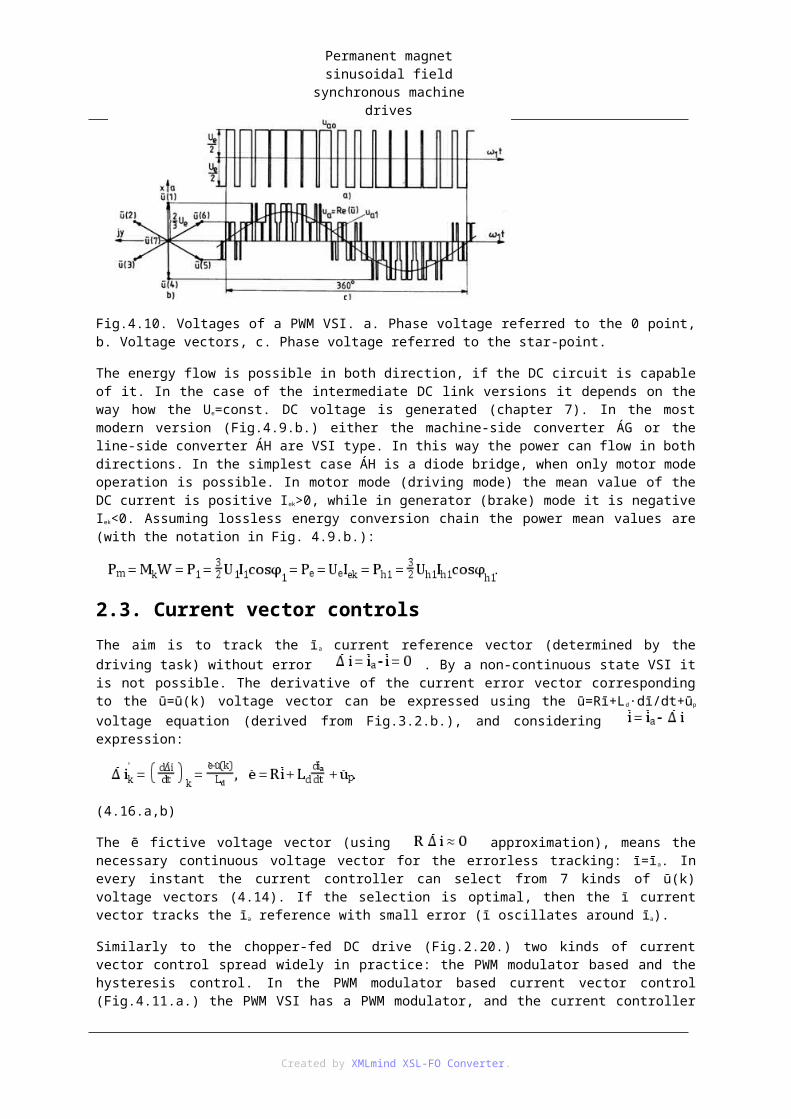
Fig.4.10. shows a characteristic inverter voltage time function.
Fig.4.10. Voltages of a PWM VSI. a. Phase voltage referred to the 0 point, b. Voltage vectors, c. Phase voltage referred to the star-point.
The energy flow is possible in both direction, if the DC circuit is capable of it. In the case of the intermediate DC link versions it depends on the way how the U e=const. DC voltage is generated (chapter 7). In the most modern version (Fig.4.9.b.) either the machine-side converter ÁG or the line-side converter ÁH are VSI type. In this way the power can flow in both directions. In the simplest case ÁH is a diode bridge, when only motor mode operation is possible. In motor mode (driving mode) the mean value of the DC current is positive I ek>0, while in generator (brake) mode it is negative I ek<0. Assuming lossless energy conversion chain the power mean values are (with the notation in Fig. 4.9.b.):
2.3. Current vector controlsThe aim is to track the īa current reference vector (determined by the driving task) without error
. By a non-continuous state VSI it is not possible. The derivative of the current error vector corresponding to the ū=ū(k) voltage vector can be expressed using the ū=Rī+L d·dī/dt+ūp voltage equation (derived from Fig.3.2.b.), and considering expression:
(4.16.a,b)
The ē fictive voltage vector (using approximation), means the necessary continuous voltage
Created by XMLmind XSL-FO Converter.

Permanent magnet sinusoidal field synchronous machine drives
vector for the errorless tracking: ī=īa. In every instant the current controller can select from 7 kinds of ū(k) voltage vectors (4.14). If the selection is optimal, then the ī current vector tracks the ī a reference with small error (ī oscillates around īa).
Similarly to the chopper-fed DC drive (Fig.2.20.) two kinds of current vector control spread widely in practice: the PWM modulator based and the hysteresis control. In the PWM modulator based current vector control (Fig.4.11.a.) the PWM VSI has a PWM modulator, and the current controller acts through this modulator indirectly. The hysteresis current vector controllers (Fig. 4.11.b.) control the PWM VSI directly. In Fig.4.7.a.,b. PWM modulator based version is assumed.
Fig.4.11. Current vector control methods. a. PWM modulator based controller, b. Hysteresis controller.
2.3.1. PWM modulator based current vector controls
The PWM modulator based current vector control (Fig.4.11.a.) has more versions, depending on in which coordinate system the components of the ī current vector are controlled, and which are the input signals of the PWM modulator. If the SZI controllers control the dq components, then the two versions in Fig.4.12.a.,b., if the abc components (phase currents), then the two versions in Fig. 4.12.d.,e. are possible. The SZI current controllers are PI type in the practice. Fig.4.12.c. presents how the components d-q are produced. The control signals (with index v) control space-vector PWM modulator in the a,e versions and three-phase PWM modulator in the b,d versions. The necessity of the coordinate transformations is obvious in all cases.
Fig.4.12. Block diagrams of the PWM modulator based current vector controls. a,b,c. Controllers in dq coordinates, d,e. Controllers in abc coordinates.
Le’s examine the versions in Fig.4.12.a. and Fig. 4.12.d. in a little bit more detail.
Current vector control with dq components, by space-vector PWM (SPWM) (Fig.4.12.a.). The detailed block diagram of this version is in Fig.4.13.
The blocks SZID and SZIQ are usually PI type current controllers, their outputs (uvd and uvq) form a control vector , which is proportional to the ū1 fundamental voltage vector of the PWM inverter (the motor), if the fISZM switching frequency is large enough. According to the experience, if f ISZM>20f1 then ū1=Kuūv. As a synchronous machine is investigated, the maximal value of f 1 is determined by the maximal speed (n=n1=f1/p).
Created by XMLmind XSL-FO Converter.

Permanent magnet sinusoidal field synchronous machine drives
In practice: f1max≤100Hz, so with fISZM≥2kHz the above proportionality is well correct. The input signals of the SPWM are the uv amplitude and αv angle of the ūv control vector, its output signals are the two-level va, vb, vc inverter control signals. In practice, the SPWM is operating in sampled mode, the sample frequency is equal to the fISZM frequency.
Fig.4.13. Current vector control with dq components, by SPWM.
Fig.4.14. Voltage vectors. a. Creation of ū1(n) in sector 1, b. The 60° wide sectors.
Using sampled SPWM in the nth sample period with the control vector
(4.17.a,b,c)
fundamental voltage vector is prescribed. Ku is the voltage gain factor of the SPWM controlled VSI. The ū1(n) vector can be produced by switching on the neighbour three ū(k) voltage vectors (Fig. 4.14.b) for proper time interval. In the time instant presented in Fig.4.14.a. the ū1(n) is in the sector 1 of 60° degree.
Here ū(1), ū(2) and ū(7) are the three neighbour vectors. The ū1(n) vector is developed as the time weighted mean value of these vectors:
(4.18)
Where τ1n+τ2n+τ7n=τ=const. is the sampling period, b1n+b2n+b7n=1 is the sum of the duty cycles. The b1n, b2n and b7n
duty cycles can be derived from the geometric considerations based on Fig.4.14.a.:
Created by XMLmind XSL-FO Converter.

Permanent magnet sinusoidal field synchronous machine drives
(4.19.a,b,c)
Where U1max is the possible maximum fundamental peak value, which is according to Fig.4.14.a. is:
(4.20)
The function of the duty cycles in sector 1 is presented in Fig.4.15. for 0,8U1max amplitude ū1 fundamental voltage. b1n and b2n are proportional to the prescribed u1(n)=0,8U1max amplitude, the b1n/b2n ratio depends on the α1(n) angle. The switching between the 3 possible vectors can be done in two ways (Table 4.2.).
Fig.4.15. The angle dependency of the duty cycles in sector 1 with u1(n)/U1max=0,8.
Table 4.2. Switching methods in sector 1.
Method I. Method II.
k 1 2 7 1 2 7 1 2 7 1 2 7P 2 1 7N 1 2 7P
sample n n+1 n+2 n n+1 n+2
There is one double switch at method I. in every sampling period, even by 7P or by 7N the ū(7)=0 voltage vector is produced. It is eliminated using method II. by the periodical changing of the switching order of ū(1), ū(2), 7P and 7N. Considering Table 4.2. and Fig.4.14.b. it can be established, that at method I. 4, at method II. 3 switchings correspond to one sampling period. I.e. using method II. the switching number can be reduced to ratio ¾ and also the switching loss proportional to it, comparing with method I.
The operation of the SPWM is investigated in sector 1, but it operates in the other sectors similarly.
Current vector control with abc phase quantities, by three-phase PWM modulator (3-Ph PWM) (Fig.4.12.d.).
Created by XMLmind XSL-FO Converter.

Permanent magnet sinusoidal field synchronous machine drives
Fig.4.16. Current vector control with abc phase quantities, by 3-Ph PWM.
Fig.4.17. Three-phase analogue PWM modulator
Fig.4.18. Operation of the analogue PWM modulator (fΔ/f1=9).
The SZIA, SZIB and SZIC are usually PI type current controllers, their output signals are the u va, uvb and uvc
phase control signals (modulating signals). Processing them the 3-Ph PWM generates the two-level control signals va, vb, vc for the inverter. The 3-Ph PWM consists of 3 one-phase modulator, but the carrier wave of the modulators (uΔ) is common (Fig.4.17.).
Operation of the analogue PWM modulator is demonstrated in Fig.4.18. for phase a. (Nowadays digital modulators implemented by counters are applied.) While uva>uΔ, then va=H (high level), phase a is on the P bar: ua0=+Ue/2. When uva<uΔ, then va=L (low level), phase a is on the N bar: u a0=-Ue/2. There exist fΔ/f1=const. synchronous modulation and, fΔ=const., fΔ/f1=var. asynchronous modulation. It can be proved, that in steady-state in the output voltage of the inverter besides the fundamental component with frequency f 1 upperharmonics with frequencies fΔ±2f1, fΔ±4f1,…, 2fΔ±f1, 2fΔ±3f1,… also appear.
The synchronous machine thanks to its Ld synchronous inductance is very good filter for the current and the torque. It is demonstrated in Fig.4.19. drawn according to Fig. 4.2. Here Δū and Δī are the resultants of the upperharmonics:
Created by XMLmind XSL-FO Converter.

Permanent magnet sinusoidal field synchronous machine drives
(4.21.a,b,c)
Where ν is the order number of the harmonics. It is assumed, that the ū p pole voltage (4.2) is purely fundamental (ω1=2πf1=w1=w). If fΔ≥2kHz, then well approximately the current pulsation ( ) and the torque pulsation (Δm) caused by can be neglected (it is also true for modulation method in Fig.4.13., if f ISZM≥2kHz). The cage-rotor induction machine (chapter 5.) is also a good filter if PWM VSI is the supply.
Fig.4.19. Equivalent circuits. a. For instantaneous values, b. For fundamental values, c. For harmonics.
It is true with good approximation either for synchronous or asynchronous modulation that the VSI controlled by 3-phase PWM modulator can be considered as a proportional element if fΔ/f1>20. E.g. for phase a:
(4.22.a,b)
According to Fig.4.18. maximum of uva may be UΔ m/2, consequently the maximal fundamental peak value is:
(4.23)
Comparing with (4.20) it is clear that the maximal fundamental voltage with 3-phase PWM modulator is 15% less than with SPWM. The utilization of the inverter can be improved if the 3-phase PWM is controlled by modified (uv*) control signals (Fig.4.20).
Fig.4.20. Modification of the control signals with zero sequence components.
If the control signals are modified in the way presented in Fig.4.20., then the voltage amplification factor is
increased to and so as with SPWM.
2.3.2. 4.2.3.2 Hysteresis current vector controls
The hysteresis current vector controls operate the VSI directly (without PWM modulator). As the control is fulfilled with vectors, instead of tolerance band tolerance area should be given. It can operate in stationary or pole-field coordinate system. The tolerance area in stationary coordinate system can be a circle or a regular hexagon, in pole-field coordinate system can be circle or square. The operation can be analogue or digital.
Analogue control in stationary coordinate system is investigated in the following. The analogue hysteresis current vector controller senses that instant (comparing instant), when the current error vector ( )
Created by XMLmind XSL-FO Converter.
Permanent magnet sinusoidal field synchronous machine drives
reaches the border of the tolerance area. It means the condition at ΔI radius tolerance circle, at hexagon with 2ΔI side distance: │Δia│=ΔI or │Δib│=ΔI or │Δic│=ΔI conditions (Δia=iaa-ia, Δib=iba-ib, Δic=ica-ic are the phase current errors). The tolerance area is circle in Fig.4.21.a. and hexagon in Fig.4.21.b. After sensing the reaching of the tolerance band the adaptive version a two-step procedure selects the optimal voltage vector ū(k) from the possible seven switchable ones by the VSI.
Fig.4.21. Tolerance areas. a. Circle, b. Hexagon.
The block diagram of the adaptive hysteresis current vector control is given in Fig.4.22. The comparing and
convergence conditions are valid for circle shape tolerance area (Fig.4.23.). is the derivative of the current error vector corresponding to the ū(k) voltage vector at the t0 comparing instant (4.16.a), ‘·’ means scalar
product. According to Fig.4.23., is the condition to move current error vector back to the tolerance area by the ū(k) voltage vector. According this vector convergence condition the algorithm selects among the available seven ū(k) voltage vectors (4.14) the possible N vectors. Usually N>1, so a criterion is necessary to select the optimal. E.g. the criterion given in Fig.4.22. (max(T k/Sk)) has the aim to get less switching (Sk) and more Tk for staying inside the tolerance area.
Fig.4.22. Block diagram of the adaptive hysteresis current vector control.
Fig.4.23. The comparing instant with circle shape tolerance area.
Let’s assume that Fig.4.24. corresponds to the t0 comparing instant. Fig.4.24.a. corresponds to (4.16.a), in
Created by XMLmind XSL-FO Converter.

Permanent magnet sinusoidal field synchronous machine drives
Fig.4.24.b. the dotted lines are the derivatives (speeds) of the current error vector at point, the numbers are the k values in ū(k). According to Fig.4.24.a,b. the following can be established: ūold=ū(2), N=3: ū(1), ū(6), ū(5), the switching numbers are: with selecting ū(1): S1=1, with selecting ū(6): S6=2, with selecting ū(5): S5=3, the relation of the expected times to the next comparing is T1>T6>T5. Considering these, using the max(Tk/Sk)) criterion: ūnew=ū(1) should be selected. The adaptive hysteresis current vector control described in Fig.4.22. is quite complicated, consequently it is not applied in practice.
Fig.4.24. The vectors in the comparing instant. a. Voltage vectors. b. Current error vectors.
In the practically widely applied simple hysteresis current vector control the ū new voltage vector depends on the current error vector only. In the simplest hexagon shape tolerance case selection of ū(k) depends on
the Δiao, Δibo és Δico phase current errors. This is the 3-phase bang-bang current control (Fig.4.25.).
Fig.4.25. Block diagram of the three-phase bang-bang current control.
Only phase a is detailed, since circuits of the phase b and c are similar. It can be proved, that because of the interaction of the phases coming from ia+ib+ic=0 the error per phase can be larger (max. ±2ΔI) then the tolerance band ±ΔI. It means, that the vector convergence condition for hexagon is not always satisfied. Consequently the ī current vector can move to the shaded triangles around the tolerance area (Fig.4.21.b.). This control is simple and robust, only the ΔI phase tolerance band must be set, taking into consideration the allowed switching frequency of the inverter. Note: if the 0 and 0’ point would have been connected (Fig.4.25.), then the current bang-bang controls in the phases would be independent, so the phase current errors would stay in the ±ΔI band.
Created by XMLmind XSL-FO Converter.

5. fejezet - Frequency converter-fed squirrel-cage rotor induction machine drivesThe rotor ‘winding’ is a short-circuited squirrel-cage (shortly: cage). The cage rotor induction machine can be substituted by a wounded rotor machine, which has short-circuited rotor coils with terminals ra, rb, rc (Fig.3.1.a.) so the rotor terminal voltage is zero: ūr=0. Considering this and (3.6.c), the rotor voltage equation in
rotor coordinate system (wk=w) shows, that the īr rotor current vector can modify the rotor flux vector only:
(5.1.a,b)
The flux linked with the short-circuited rotor coil can be modified only slowly because of the small R r
rotor resistance. The rotor flux vector must be developed by the ī stator current. The constant rotor flux field-oriented controls are examined in the following.
1. Field-oriented control methodsThe operation of the cage rotor induction machine depends on the flux linked with the short-circuited rotor principally. Accordingly the flux equivalent circuits (Fig.3.3.a. and Fig.3.4.a.) should be used and the coordinate
system should be fixed to the rotor flux vector (Fig.5.1).
Fig.5.1. The ī stator current in the coordinate system fixed to the rotor flux.
Fig.5.2. Development of the rotor flux.
The equations (3.6.a-d) must be actualized, by using wk=wψr=dαψr/dt and ūr=0:
stator:
(5.2.a,b)
rotor:
Created by XMLmind XSL-FO Converter.

Frequency converter-fed squirrel-cage rotor induction machine
drives
(5.2.c,d)
Where wr=wψ r-w is the angular speed of the rotor flux vector relatively to the rotor. In the coordinate system fixed to the rotor flux vector (so called field coordinate system):
(5.3.a,b,c)
Decomposing the rotor voltage equation (5.2.c) to d real and q imaginary parts:
(5.4.a,b)
(5.5.a,b)
Decomposing the rotor flux equation (5.2.d) to real and imaginary parts and considering (5.4.b) and (5.5.b):
(5.6.a,b)
(5.7.a,b)
(5.6.b) shows that the rotor flux vector amplitude (ψ r) can be modified by the id flux producing component only, iq has no effect on it. Modifying id, ψr tracks the Lmid value like a first order lag elemet with T ro time constant, caused by the flux modification damping effect (5.4.b) of the short-circuited rotor (Fig.5.2.). So the ψ r
amplitude can only be modified slowly, as the T ro=Lm/Rr no-load rotor time constant is more tenth of sec. Consequently for a high dynamic drive the rotor flux amplitude (ψr) should be kept constant. Then as dψr/dt=0 and ψr=Lmid:
(5.8.a,b,c,d)
The torque with Park-vectors (3.8.a), considering (5.2.b) is:
(5.9)
(5.10)
(5.10) shows, that the m torque can be set by the iq torque producing current component. For m>0, iq>0
(Fig.5.1.), for m<0, iq<0. From (5.7.b) the angular speed of the rotor flux vector relatively to the stator can be expressed:
Created by XMLmind XSL-FO Converter.

Frequency converter-fed squirrel-cage rotor induction machine
drives
(5.11)
As can be seen from (5.6.a) and (5.10), the supply of the cage rotor induction machine should be oriented to the
rotor flux vector (shortly to the field).
The block diagram of the current source supplied cage rotor induction machine in field coordinate system is drawn using Fig.5.3 (1.1.a, 5.6.b, 5.10 and 5.11). The figure is extended by the i a,ib,ic→ix,iy→id,iq transformation boxes. According to this block diagram the field-oriented current source supply must feed the induction machine with such ia, ib, ic currents (resulting in ī=(2/3)(ia+āib+ā2ic) current vector) to get id=ψr/Lm=const. d current component and the q current component (iq) must be proportional to the demanded torque.
Fig.5.3. Block diagram of the current source-fed cage rotor induction machine.
Consequently the current vector control of the induction machine in field coordinate system is decoupled to two independent i d and i q (rotor flux and torque ) control loop. The induction machine supplied in this way behaves similarly to the compensated, separately excited DC machine. The id flux producing component corresponds to the excitation current (or the permanent magnet), the iq torque producing component corresponds to the armature current, and iq modifies only the torque, in the same way as the armature current in the DC machine. It should be emphasized, that the decoupling is true only in the d-q rotor flux coordinate system. The critical point of the field-oriented control is the determination of the position of this coordinate system. The switching-on of the field-oriented drive must be started with the development of the ψ r rotor flux (as in the DC machine with the switching on of the excitation), and this flux must be kept until the switching-off the drive.
The motor voltage can be modified directly by the PWM VSI in practice. The field-oriented control can be implemented by voltage source supply also, if the ū voltage vector necessary to develop the previously defined id, iq currents is connected to the motor. For the investigation of the voltage source supply, let’s substitute the (5.2.b) expression of the stator flux vector into (5.2.a):
(5.12)
The real and imaginary parts of the voltage equation are:
(5.13.a)
(5.13.b)
As can be seen, the decoupling is not exact for the voltages in field coordinate system, since the d axis equation contains q quantity, the q axis equation contains d quantity also (there is a cross-coupling). Dividing the ud and uq
voltages by R and arranging, the following equations are got:
Created by XMLmind XSL-FO Converter.

Frequency converter-fed squirrel-cage rotor induction machine
drives(5.14.a)
(5.14.b)
Fig.5.4. Block diagram of the voltage source supplied cage rotor induction machine.
The id and iq currents track the left side quantities with T’=L’/R stator transient time constant (it is few 10 ms, i.e. less than the TR0 by one order). The block diagram in Fig.5.4. is drawn using these two equations and Fig.5.3. (the dotted box here corresponds to the part of Fig.5.3. surrounded by dotted line). As can be seen in the block diagram, e.g. the modification of iq component (the m torque) requires not only the modification of u q, but the modification of ud also, if the id component (the ψr flux) should be kept constant. As the inverter acts in stationary coordinate system by ua, ub, uc voltages, the block diagram in d-q coordinate system is extended by the abc/xy and the xy/dq transformations.
2. Steady-state sinusoidal field-oriented operationAlso the steady-state symmetrical sinusoidal operation can be got from the equations derived in the previous chapter. In the case of inverter supply, the statements are valid for the fundamental quantities with f 1 frequency. Capitals denote steady-state values, index 1 denotes fundamental quantities in the following. The summarised equations of the Ψr1=LmI1d=const. operation are the following:
(5.15.a,b)
(5.16.a,b)
(5.17.a,b,c)
(5.18.a,b)
Using these equations and assuming Ψr1=Ψrn=const. nominal rotor flux, the current vector diagram (Fig.5.5.a.) and the mechanical characteristics (Fig.5.6.a.) are drawn. It comes from (5.18.a) and (2.6.a) that the W(M) mechanical characteristics (Fig.2.2. and Fig.5.6.a.) are similar to that of the DC machine, but the role of the U terminal voltage is played by f1 frequency, the role of the ϕ flux is played by the Ψr1 rotor flux, and the R armature resistance must be substituted by the R r rotor resistance. The Fig.5.5.b. and Fig.5.6.b. are for Ψ1=Ψn=const. nominal stator flux operation (without deduction).
Created by XMLmind XSL-FO Converter.

Frequency converter-fed squirrel-cage rotor induction machine
drives
Fig.5.5. Current vector diagrams. a. Ψr1=const. operation, b. Ψ1=const. operation.
Fig.5.6. Mechanical characteristics. a. Ψr1=Ψrn operation.
Fig.5.6. Mechanical characteristics. b. Ψ1=Ψn operation.
The W(M) curves are for abc positive phase sequence supply, the acb phase sequence case can be got by reflecting the curves to the origin. Modifying the f1 frequency, the W(M) curves are shifted parallel. The Ψr1=const. rotor flux operation is more advantageous, since then the W(M) mechanical characteristics have not a
break-down point (at Ψ1=const.: and at Ψ1=Ψn: Mb=(2-2,5)Mn). Above the nominal f1n frequency neither the rotor flux (Ψr1) nor the stator flux (Ψ1) amplitude can be kept at the nominal value. The reasons are:
1. The inverter cannot provide significantly larger voltage than U1n=Un nominal voltage, and the motor could not withstand it too.
Created by XMLmind XSL-FO Converter.

Frequency converter-fed squirrel-cage rotor induction machine
drives2. The stator core losses (PcoreH hysteresis and PcoreE eddy-current losses) can reach not allowed value:
(5.19)
Accordingly, in the range f1>f1n (W1>W1n) the flux must be reduced, the field must be weakened. E.g. the Ψr1 rotor flux must be modified approximately in the following way in the field-weakening W1>W1n (approx. W>Wn) range:
(5.20)
Fig.5.5.a. and Fig.5.6.a. correspond to Ψ r1=Ψrn normal operation. Fig.5.7. shows the field-weakening ranges also (assuming 4/4 quadrant operation) on the W(M) plane (Fig.5.7.a.) and the Ī 1 current vector ranges in the d-q coordinate system (Fig.5.7.b.).
Fig.5.7. Ranges extended by the field-weakening operation. a. W(M) plane, b. Ranges of the Ī1 current vector.
3. Implementation methods of the field-oriented operationThe aim is to keep the ψr amplitude constant by closed-loop regulation or by open-loop control. There are two widely spread methods in practice:
Direct rotor flux control. In this case the ψr amplitude and αψ r angle of the rotor flux vector (Fig.5.1)
(5.21)
is created (usually by a machine model). The ψ r rotor flux amplitude is kept through id by control, and the m torque is controlled by iq. This method is implemented by current vector control oriented to the rotor flux vector (shortly field-oriented current vector control). Only this practically widely applied closed-loop regulated version is investigated in the following.
Indirect rotor flux control . In this case the ψr and αψ r are not created directly, and ψr is not regulated in closed-loop, only it is kept by open-loop control. There will be an example for this method at the current source inverter-fed drives (Chapter 8).
3.1. Field-oriented current vector control
Created by XMLmind XSL-FO Converter.

Frequency converter-fed squirrel-cage rotor induction machine
drivesThe block diagram of the drive controlling the torque by field-oriented control in given in Fig.5.8. From the m a
torque reference the reference value of the torque producing current component can be derived using (5.10):
(5.22)
According to (5.20) the reference value of the rotor flux in the simplest case depends on the wψ r=w1=2πf1
fundamental angular frequency (approximately on the w speed) (Fig.5.9.a.):
(5.23.a,b)
Fig.5.8. Field-oriented torque-controlled drive. a. By SZΨ flux controller., b. By SZU voltage controller.
The SZΨ flux controller provides the reference value of the flux producing current component: i da. If there is only normal operation (Fig.5.7.a.), then the SZΨ can be omitted, and ida=Idn=Ψrn/Lm=const. flux producing current reference can be set. Similarly to Fig.4.5., a SZU voltage controller controlling the fundamental voltage vector amplitude (u1) also can provide the ida reference value (Fig.5.8.b.). It controls to u1=Un in the field-weakening range, its upper limit must be set to Idn, its lower limit must be set to Idmin (Fig.5.7).
In energy-saving operation, the ψra flux reference can depend on the load (on the m a torque reference). The torque expression (5.10) with ψr=const. operation by substitutions ψr=Lmid, id=icosϑ and iq=isinϑ can be written in the following form:
(5.24.a,b)
Created by XMLmind XSL-FO Converter.

Frequency converter-fed squirrel-cage rotor induction machine
drivesFig.5.9. Refrences. a. Rotor flux reference. b. Current references at m a=const.>0. c. Dynamic and energy-saving current references.
As coming from (5.24.a), for m=const. torque the idiq product is constant, i.e. it is a hyperbolic function on the id-iq plane. It is demonstrated in Fig.5.9.b. for current references (at the permanent magnet synchronous machine for m=const. torque the iq is constant according to (4.8)). As can be seen in (5.24.b), a m>0 torque can be developed with the minimal current with ϑ=45° torque angle. Since besides the dependent
copper losses there are core losses also depending on , the maximal efficiency energy-saving operation for m>0 is at ϑopt>45°. ϑopt depends on the f1 frequency, since the core losses (5.19) are frequency dependent also. Near f1≈0 frequency: ϑopt≈45°, since the core losses are zero, near f1≈f1n frequency: ϑopt≈60°. If independently of the frequency the torque angle is kept at ϑn=arctg(Iqn/Idn)=arctg(WrnTro) corresponding to the N nominal point (f1n, Ψrn=LmIdn, Mn=(3/2)ΨrnIqn) (Fig.5.9.c.), then a suboptimal energy-saving operation is got (it means ϑ=ϑn, Wr=Wrn rotor frequency). In this case the current references at m>0, |w|<W n depend on the torque reference in the following way:
(5.25.a,b)
The operation is similar to the series excited DC machine.
If good dynamics is the goal, then ida=Idn=const. is necessary in the a normal range.
Fig.5.10. Equivalent circuit (wk=0).
By the two-level VSI (Fig.4.9) it is again not possible to track the reference value without error (). Fig.5.10. is redrawn from Fig.3.4.b. From the corresponding voltage equation
(ū=Rī+L’dī/dt+ū’), substituting , the derivative of the current error vector for the ū=ū(k) voltage vector can be expressed (wk=0):
(5.26)
The ū’ transient voltage can be calculated from (5.21):
(5.27)
The first term is zero in the ψ r=Ψrn=const. normal range. A well operating current vector controller selects from the available seven ū(k) voltage vectors (4.14) that one, which results in small current error and small switching frequency.
Similarly to the permanent magnet synchronous machine the current references are available in d,q and the feedback signals are in a,b,c components and “same type” reference and feedback signals are necessary for the current vector control. The possibilities are demonstrated in Fig.5.11. which is very similar to Fig.4.6.
Created by XMLmind XSL-FO Converter.

Frequency converter-fed squirrel-cage rotor induction machine
drives
Fig.5.11. Current vector coordinates. a. Current reference vector diagram. b. Coordinate transformation chain.
At the cross-sections a,b,c,d,e, in the possible two coordinate systems, five different “same-type” reference and feedback signal combinations can be considered. Accordingly the following current vector controls can be implemented theoretically:
a section: coordinate system rotating with the rotor field, Cartesian coordinates,
b section: coordinate system rotating with the rotor field, polar coordinates,
c section: stationary coordinate system, polar coordinates,
d section: stationary coordinate system, Cartesian coordinates,
e section: stationary coordinate system, phase quantities.
It can be established, that the coordinate transformation cannot be avoided, and for the stationary→rotor field
and the rotor field→stationary coordinate transformations the αψ r angle of the rotor flux vector must be known. In practice, the a, or the e versions are used for current vector control (Fig.5.12.). In version a the references (ida, iqa), in version e the feedback signals (ia, ib, ic) can be used directly. In version a two, in version e one coordinate transformation is necessary. Comparing Fig.5.12.a,b. with Fig.4.7.a,b. the high similarity between the current vector control of the cage rotor induction machine and the permanent magnet synchronous machine can be seen. The only one but significant difference comes from the fact, that different flux vector is
used for the field orientation. At the PM synchronous machine it is the pole flux vector rotating with the rotor. Its angle (α) can be measured by a position encoder (P), its amplitude in ideal case is constant
(Ψp=const.). At the cage rotor induction machine it is the rotor flux vector, neither its αψ r angle nor its ψr amplitude can be measured directly. These can be produced by a machine model.
Fig.5.12. Block diagram of the current vector controla. In rotor field coordinate system with Cartesian coordinates (version a), b. In stationary coordinate system with phase quantities (version e).
At the cage rotor induction machine the PWM modulator based and hysteresis current vector control methods (Fig.4.11.a,b.) also can be applied. Also the PWM modulator based methods in Fig.4.13. and Fig.4.16. are used
Created by XMLmind XSL-FO Converter.

Frequency converter-fed squirrel-cage rotor induction machine
driveswidely in the practice. Thanks to the high similarity, universal drives are developed (UNIDRIVE), capable of current vector control of either PM synchronous machine or cage rotor induction machine.
3.2. Machine modelsA new component has appeared in Fig. 5.12.a,b: the machine model. The machine model manipulates measured signals and machine equations (Fig.5.13.) The machine equations need machine parameters. The parameters can be determined off-line (before operation, off-line identification) or on-line (during operation, on-line identification). These two methods are frequently applied together.
Fig.5.13. How the machine model is interfaced with the induction machine.
There are two models applied widely in the practice: the stator model and the rotor model. It should be considered in both of them, that the measurement can be done only in stationary coordinate system (wk=0).
Stator model. Using the stator voltage equation (3.6.a) with wk=0 and Fig.3.4.a., the x and y components of the rotor flux vector ( ) can be calculated:
(5.28.a,b)
(5.29.a,b)
The machine model in Fig.5.14. uses these equations. Besides the α ψ r angle of the rotor flux vector it provides the angular speed (wψ r=dαψ/dt), the ψr amplitude and the m electromagnetic torque. The machine model uses the measured voltages and currents, and machine parameters R and L’. It is enough to measure two line-to-line voltages and two line currents in practice. At low f 1 frequency the term Rī is significant relatively to ū, so the inaccuracy of R stator resistance (caused by the temperature) can result in large error. The open-loop analogue integrators calculating ψx and ψy flux components have error caused by the offset and drift. Consequently this model has a lower frequency limit in the practice (approx. 0.05f1n=0.05 50=2.5 Hz). Because⋅ of these problems this model is not applied in servo and electric vehicle drives.
Fig.5.14. Stator machine model.
Rotor model. The rotor voltage equation (3.6.c) is the starting point. w k=0 and ūr=0 are substituted, and the not
measurable rotor current is eliminated by (3.6.d):
Created by XMLmind XSL-FO Converter.

Frequency converter-fed squirrel-cage rotor induction machine
drives
(5.30)
The x and y components of can be expressed:
(5.31.a)
(5.31.b)
The machine model in Fig.5.15. uses these equations. It uses the measured the currents and speed, calculates the ψr , αψ r, wψ r and m signals using the Lm, Rr and Tro=Lm/Rr machine parameters. It has a great advantage against to the previous one: it does not contain open-loop integration. The negative feed-backed integrators result in first order lag elements (the time constant is Tr0), so the offset and drift problems are avoided. This model can operate even until zero frequency. There are problems associated with the variation of the R r rotor resistance (caused by the temperature, it is a slow process) and the variation of the Lm magnetizing inductance (caused by the variation of saturation in the field-weakening range, it is a much faster process). In a sophisticated drive on-line identification is necessary to get the actual value of R r and Lm. If the Rr and Lm parameters used in the model are inaccurate, then the calculated ψr and αψ r values do not correspond to the actual values in the motor. Consequently the field-oriented control uses these inaccurate values, so the control is done not exactly in rotor flux coordinate system, the decoupling in the current components id and iq is deteriorated.
Fig.5.15. Rotor machine model.
There is a combined model also, which produces not only the rotor flux, but the w speed also. If the rotor
voltage equation (5.30) is multiplied by the conjugate of the rotor flux vector ( ), the folloving vector equation is got:
(5.32)
The x real and y imaginary components are:
(5.33.a)
(5.33.b)
Created by XMLmind XSL-FO Converter.

Frequency converter-fed squirrel-cage rotor induction machine
drivesThe w speed can be expressed from the imaginary component:
(5.34)
This expression makes possible to calculate the speed without mechanical sensor (sensorless). The ψ rx and ψry
flux components are calculated by (5.29.a,b), the w speed is calculated by (5.34) in Fig.5.16. The stator voltages and currents must be sensed. (5.33.a) can be used for parameter identification: if the parameters R, L’, R r, Lm are not accurate, then vx≠0. At constant flux operation (ψr=const., Lm=const.) the vx=0 equality makes possible a simple on-line identification of one parameter, e.g. Rr.
Fig.5.16. The combined machine model calculating the rotor flux and the speed.
4. Direct torque controlConsidering (5.2.b) (at PM synchronous machine (4.3) ) the ī current vector control can be implemented by the control of the stator flux. This principle is the background of the direct flux and torque control (shortly direct torque control DTC). It is described in the following for cage rotor induction machine, since DTC is applied widely for this one.
In the most commonly used application the ma torque reference is set by the SZW speed controller (Fig.5.17.), the ψa flux amplitude reference is set by the FΨA set-point element. The ψa flux reference is practically speed dependent, in the w≤Wn range it is: ψa=Ψn, in the w>Wn range it is: ψa=(Wn/w)Ψn.
Fig.5.17. Direct flux and torque control subordinated to speed control.
Let’s substitute (5.2.b) to the torque expression of the induction machine (5.9):
(5.35.a)
Created by XMLmind XSL-FO Converter.

Frequency converter-fed squirrel-cage rotor induction machine
drives
(5.35.b)
So the torque can be calculated by the fluxes also (δ is the small angle between and ). In steady-
state in the stationary reference frame the rotor flux vector rotates with wψr=dαψr/dt≈w1=2πf1
fundamental angular frequency, while the stator flux vector can be modified by the applied ū(k) terminal voltage vector (3.6.a):
(5.36)
The two-level VSI can switch 7 kinds of ū(k) voltage vector (4.14) to the machine terminals, so in every instant
7 different kinds of flux speed vector is possible. The amplitude and angle of the
stator flux vector can be changed much faster than that of the rotor flux vector (caused by the L’ī term). The fastest torque modification can be done by changing the angle between them (d). The fastest d modification can be done by ū voltage vectors, nearly perpendicular to , since the d angle is small. E.g. at the instant demonstrated by Fig.5.18. the m>0 torque and the corresponding d>0 angle can be increased the fastest by switching the ū(1) voltage vector to the induction machine terminals. The fastest torque and d decrease can be reached by the ū(4) voltage vector. The ū(7)=0 voltage vector stops the vector, so the d angle and the torque decreases.
Fig.5.18. Voltage vectors, flux vectors and flux sectors.
Fig.5.19. Flux speed vectors (5.36).
Identifying the flux vector angular position by six 60° sectors, general rules depending on sector number (N=1,...6) can be given for the selection of the voltage vectors. The flux vector sectors must be defined relatively to the ū(1), … ū(6) voltage vectors according to Fig.5.18. Neglecting the R resistance, the possible
flux speed vectors are identical with the ū(k) voltage vectors. For examining the ith sector, the ū(1), … ū(6) voltage vectors are identified as in Fig.5.19. (the indices overflow at 6). Let’s assume w y r>0 and m>0 motor operation. By eq. (5.36) geometrically can be proved, that if the flux vector is inside the sector, then the absolute value of the flux vector is increased by the ū(i), ū(i+1) and ū(i+5), while decreased by the
Created by XMLmind XSL-FO Converter.
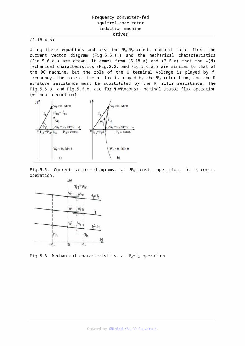
Frequency converter-fed squirrel-cage rotor induction machine
drivesū(i+3), ū(i+2) and ū(i+4) voltage vectors. In the same time, the torque (the d angle) is increased by ū(i+1) and ū(i+2), while decreased by ū(i+4) and ū(i+5) voltage vectors. The ū(7) zero voltage vector does not change the flux, but decreases the torque.
This direct flux and torque control keeps both the stator flux vector amplitude and the m torque in a prescribed band by bang-bang control. The voltage vector to be switched to the induction machine is determined by three signals: the Δψ=ψa-ψ flux amplitude error, the Δm=ma-m torque error, and the angular position of the flux vector given by the sector number N. A possible block diagram of the control scheme is given in Fig.5.20.
Fig.5.20. Direct flux and torque control.
The generation of the ya flux amplitude reference and the ma torque reference is not given in the figure. The SZY flux controller is a two-level hysteresis comparator, the SZM torque controller is a three-level hysteresis comparator. So the possible values of KY are 1 and 0, the possible values of a KM are 1, 0 and -1. The block ARC determines the actual sector of from yx and yy components. The machine model is a simplified version of the stator model in Fig.5.14., since the y r and ay r are not needed now. The torque is calculated with the m=(3/2)(ψxiy–;ψyix)expression.
By the rules determined for the ith sector, in the function of KY, KM and N, the identifying number of the necessary ū(k) voltage vector can be given (Table.5.1.a.). The ū(7)=0 vector can be generated in two ways: all phases are connected to the P bar (7P) or to the N bar (7N), see Fig.4.9.a. This table is the Switching Table in Fig.5.20. The digitally stored table is addressed by a 6-bit binary number composed from KY (1 bit), KM (2 bits) and N (3 bits).
Table 5.1.a. The identifying numbers of the ū(k) voltage vector.
Table 5.1.b. The identifying numbers of the ū(k) voltage vector, if the ū(7)=0 vector is not used.
KY KM N KY KM N
1 2 3 4 5 6 1 2 3 4 5 6
Created by XMLmind XSL-FO Converter.

Frequency converter-fed squirrel-cage rotor induction machine
drives
1 1 2 3 4 5 6 1 1 1 2 3 4 5 6 1
0 7P 7N 7P 7N 7P 7N 0 6 1 2 3 4 5
-1 6 1 2 3 4 5 0 1 3 4 5 6 1 2
0 1 3 4 5 6 1 2 0 5 6 1 2 3 4
0 7N 7P 7N 7P 7N 7P
-1 5 6 1 2 3 4
The flux vector path of the direct flux and torque control using Table 5.1.a. as switching table is given in Fig.5.21. for the sector N=6, with w>0 and m>0 operating point qualitatively. The switchings are initiated by the flux controller in points A,B,C, while in points by the torque controller. In points A and C: Dy=-DY, so KY changes from 1 to 0, in point B: Dy=+DY, so KY changes from 0 to 1. Accordingly between points A and B: KY=0, between points B and C: KY=1. In the points on the flux vector path: KM=0, else: KM=+1. The changing of the flux vector sector alone does not cause switching. From the ū(7P)=ū(7N)=0 voltage vectors that one is selected, which causes less switching number (Table 5.1.a.). Using the direct flux and torque control in Fig.5.20., only the references and the tolerance bends can be set, consequently the control is robust. In a practical implementation the tolerance bands (±ΔM and ±ΔΨ) are ±(0.01-005) in per-unit. Generally the torque has larger band than the flux (DM>DY). The minimal value of the DM and DY bands is determined by the allowed switching frequency of the inverter.
The switch-on of the drive must be started by the development of the flux for the DTC also. KM must be set to 1, N to any value (1, 2,…6), and the derivative of the flux reference (dψa/dt) should be limited to limit the flux producing current also. The ma torque reference may be enabled only after the development of the flux.
Fig.5.21. Path of the flux vector in sector N=6.
By the ū(7) voltage vector the positive m>0 torque is decreased at wψ r>0, while it is increased at wψ r<0. It can be seen clearly in Fig.5.22.a. ū(7)=0 stops the flux vector (5.36). In this case, if wψ r>0, then angle δ and the m torque decreases (5.35.b), if wψ r<0, then angle δ and the torque m increases. Consequently, at wψ r>0 the rows KM=+1 and 0 act in Table 5.1.a., at wψ r<0 the rows KM=-1 and 0 act. As a result at wψ r>0 the torque error is not negative: Δm=ma-m≥0, at wψ r<0 it is not positive: Δm≤0 (Fig.5.22.b.). Accordingly the mean value of the torque (mk) at wψ r>0 is smaller by approx. ΔM/2, at wψ r<0 is greater by approx. ΔM/2 than the ma>0 torque reference.
Fig.5.22. The effect of the ū(7)=0voltage vector at m>0 torque. a. Flux vector diagram, b. Torque time function.
It is an advantage of the described version (capable of 4/4 quadrant operation), that it controls the torque fast,
Created by XMLmind XSL-FO Converter.

Frequency converter-fed squirrel-cage rotor induction machine
drivesand the controllers are robust.
It can be proved, that in a one rotation direction (wψ r>0) 2/4 or 1/4 quadrant drive (e.g. in a wind turbine generator) the KM=-1 rows of Table 5.1.a. are never used. So in this case the SZM hysteresis torque controller also can be two-level comparator.
There is such a Switching Table (Table 5.1.b.), where the ū(7)=0 voltage vector is not used. In this case the SZM controller is ab ovo two-level comparator. This strategy should be used in that case, when the torque (the d angle) must be controlled fast. Easily can be proved, that this strategy significantly increases the switching number.
Besides the cage rotor induction machines, the DTC is also applied for VSI-fed PM synchronous and double-fed induction machine drives in the practice.
Created by XMLmind XSL-FO Converter.

6. fejezet - Double-fed induction machine drives by VSIThe 3-phase wounded rotor slip-ring induction machine (Fig.6.1.a.) can be supplied from two side (stator and rotor sides). In sinusoidal symmetrical steady-state operation its speed can be modified by the stator and rotor frequency (f1 and fr=f2):
(6.1)
The sign of f2 is positive, if the phase sequences in the stator and the rotor are the same, and negative, if they are opposite. The powers can be expressed in the following way:
(6.2.a,b,c)
P1 is the stator terminal (input) power, P t is the stator cupper loss, Pcore is the stator core loss, Pl is the airgap power, Pr is the rotor power, Pm is the mechanical power, Ptr is the rotor cupper loss, Pcore r is the rotor core loss, P2
is the rotor terminal power. Neglecting the losses:
(6.3.a,b,c)
The powers can be expressed by the torque and angular speeds:
(6.4.a,b,c)
Where W1=ω1/p is the angular speed of the rotating field, (ω1=2πf1 is its angular frequency), W is the rotor angular speed, Wr=W1-W=ω2/p is the angular speed of the rotating filed relative to the rotor (ω2=2πf2), s=Wr/W1
is the slip. 2p=2 pole number is assumed in the following, so the angular speeds and angular frequencies are identical.
Fig.6.1. Double-fed induction machine. a) Slip-ring induction machine.
Fig.6.1. Double-fed induction machine. b) VSI supply.
Created by XMLmind XSL-FO Converter.

Double-fed induction machine drives by VSI
In the modern version of the double-fed induction machine (Fig.6.1.b.) the stator is connected directly to the lines (f1=fh=50Hz, W1=2πf1 314/s), while to the rotor a VSI is connected. Both the machine-side (ÁG) and line-≌side (ÁH) converters are two-level VSIs. Neglecting the losses and using the notations in Fig.6.1.b.:
(6.5.a,b)
The power flow is presented in Fig.6.2. for lossless case. As can be seen, in under synchronous speed (sub-synchronous) drive and above synchronous speed (over-synchronous) brake operation power is drawn from the rotor, (P2=Pr>0), while in over-synchronous drive and sub-synchronous brake operation power is supplied to the rotor (P2=Pr<0). It can be established, that the power directions are W r and M dependent. The power circuit in Fig.6.1.b. is capable of bi-directional power flow (P2>0 and P2<0), since Ue=const.>0 but Iek can be bi-directional (Iek>0 and Iek<0). If ÁG would be a diode bridge, then only P 2>0 is possible, (this is the case of the sub-synchronous cascade drive). Only the rotor power (P2=Pr=MWr) flows through ÁG and ÁH converters. Consequently they must be designed to the power (designed rating):
(6.6)
│M│max and │Wr│max are not surely developed in the same time. │M│max determines the rotor current, │Wr│max
determines the rotor voltage. A usual operation range is given in Fig.6.3. Here: W max/Wmin=2, PÁItip=MnW1/3 P≌ n/3. In this case the ÁG and ÁH converters should be designed to one-third of the nominal power of the induction machine (Pn=MnWn M≌ nW1) only, but below Wmin=(2/3)W1 speed the converter ÁG must be disconnected from the rotor, since large rotor induced voltage is developed in it.
Fig.6.2. The power flow.
Fig.6.3. A usual operation range.
As a result of the current vector control of ÁG (Fig.6.1.b.) the rotor is supplied with constrained current (current-fed). Assuming ideal lines, the stator is supplied with constrained voltage (voltage-fed) (approximately constrained flux). Consequently field-weakening is not possible in this case.
1. Field-oriented current vector controlBecause of the constrained stator flux, the rotor current vector control of the ÁG converter should be oriented to the stator flux. For the same reason, the equivalent circuit for fluxes in Fig.6.4. should be used (it corresponds to Fig.3.3.b, L’r is the rotor transient inductance).
Created by XMLmind XSL-FO Converter.

Double-fed induction machine drives by VSI
The constrained ū=ūh voltage and f1=fh=50Hz frequency means approximately flux constrain also (consider
(3.6.a) with R=0 and wk=0: ):
(6.7)
(6.8)
Because of the flux constraint the field coordinate system is fixed to the stator flux (Fig.6.5.). In this field coordinate system:
(6.9.a,b,c)
Fig.6.4. Equivalent circuit for the fluxes.
Fig.6.5. The stator flux vector ( ) and the rotor current vector (īr) in field coordinate system.
By the current Kirchhoff’s law (see Fig.6.4.) , two component equations can be given:
(6.10.a,b)
The rotor current components (ird and irq) can be controlled directly (Fig.6.1.b.), but it means indirect stator current components (id and iq) control also. According to (6.10.a), the ψ=Lm(id+ird) flux development task can be shared between the stator and the rotor flux producing current components (id and ird). The torque expression
with Park-vectors (space-vectors), considering is:
(6.12)
Created by XMLmind XSL-FO Converter.

Double-fed induction machine drives by VSI
The torque is determined by the torque producing current components (iq=-irq). With R=0 approximation, according to (6.8): . That is why approximately the iq component is proportional to the stator active power (p), while the -id component is proportional to the stator reactive power (q):
(6.14.a,b)
As can be seen, active power is demanded for torque production, and reactive power for flux production.
Coming from (6.13), the demanded torque determines the iq=-irq components only. The d current components can be chosen freely (keeping the rule (6.10.a)). If ird=Kim, then id=(1-K)im is required. Fig.6.6. shows the current vectors in field coordinate system for m=const.>0 and different K sharing constant. At K=0 the stator, at K=1 the rotor, at K=0.5 fifty-fifty the stator and the rotor develop the ψ flux. At K>1 the double-fed induction machine is over-excited, at K<1 under-excited. If R=Rr, then the minimum of the Pt+Ptr resultant cupper loss is at K=0.5.
Fig.6.6. The current vectors in field coordinate system, for m=const.>0.
The block diagram of the drive, controlling the torque by stator flux field-oriented control is given in Fig.6.7.a. The reference values of the rotor current components can be derived from the torque reference (m a) and the flux amplitude (ψ):
(6.15.a,b)
To determine irda the K sharing coefficient and the Lm magnetizing inductance must be given. Considering (6.14.b), irda can be provided by a reactive power controller also (Fig.6.7.b.).
Created by XMLmind XSL-FO Converter.
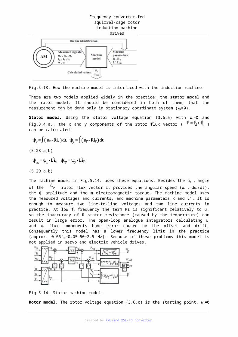
Double-fed induction machine drives by VSI
Fig.6.6. The current vectors in field coordinate system, for m=const.>0.
Fig.6.7. Field-oriented torque controlled drive. a. With irda set-point element, b. with SZQ reactive power controller.
The rotor current references are available in d,q and the feedback signals are in r a, rb, rc components. Same-type reference and feedback signals are necessary for the rotor current vector control. The possibilities are demonstrated in Fig.6.8.b. which is very similar to Fig.4.6. and Fig. 5.11.
Fig.6.8. Rotor current vector coordinates. a. Rotor current reference vector diagram. b. Coordinate transformation chain.
In the cross-sections a,b,c,d,e, in the possible two coordinate systems, five different “same-type” reference and feedback signal combinations can be considered. Accordingly the following current vector controls can be implemented theoretically:
a section: coordinate system rotating with the stator field, Cartesian coordinates,
b section: coordinate system rotating with the stator field, polar coordinates,
Created by XMLmind XSL-FO Converter.

Double-fed induction machine drives by VSI
c section: coordinate system rotating with the rotor, polar coordinates,
d section: coordinate system rotating with the rotor, Cartesian coordinates,
e section: coordinate system rotating with the rotor, phase quantities.
It can be established, that the coordinate transformation cannot be avoided, and for the rotor →stator field and the stator field→rotor coordinate transformations the αψ angle of the stator flux vector must be known. In practice, the a, or the e versions are used for current vector control (Fig.6.9.). In version a the references (ird a, irqa), in version e the feedback signals (ira, irb, irc) can be used directly. In version a two, in version e one coordinate transformation is necessary.
Fig.6.9. Block diagram of the rotor current vector control. a. In stator field coordinate system, with Cartesian coordinates (version a), b. In rotor coordinate system with phase coordinates (version e).
Comparing Fig. 6.9.a,b. with Fig.4.7.a.,b. and Fig.5.12.a.,b. the high similarity between the current vector control of the different type machines can be found.
The PWM modulator based and the hysteresis current vector control methods (Fig.3.11.a.,b.) here also can be applied. The PWM modulator based current vector control methods similar to Fig.4.13. and Fig.4.16. are applied widely in the practice.
The machine model in Fig.6.7. and Fig.6.9.a.,b. must be made in the following way. The task of the machine model is to provide the ψ amplitude and αψ angle (relative to the ra rotor axis) of the stator flux. Using the stator voltage equation (3.6.a) with wk=0 the x-y components, the amplitude and the angle of the
stator flux vector can be calculated:
(6.16.a,b)
(6.17.a,b)
The angle of the vector in the coordinate system rotating with the rotor according to Fig.6.5. is:
(6.18)
As can be seen, this calculation needs the angle of the rotor (α). In a machine model using the equations above, with the notation of Fig.5.13., the measured signals are: ua, ub, uc, ia, ib, ic and α, the used machine parameter is: R, the calculated values are: ψ and αψ.
The stator model used in chapter 5.3.2. has the same equations (5.28.a,b) as here (6.16.a,b). There the error caused by the inaccuracy of resistance R at low f1 frequency was described. It is not a problem here, since the frequency is high: f1=fh=50Hz.
Created by XMLmind XSL-FO Converter.

Double-fed induction machine drives by VSI
The direct torque and flux control can be applied for the double-fed induction machine also, (chapter 5.4.), but
here the ψr amplitude of the rotor flux vector is controlled by bang-bang control. It can be proved, that the ψra reference value is well proportional to the ψ amplitude of the stator flux vector.
Created by XMLmind XSL-FO Converter.

7. fejezet - Line-side converter of the VSI-fed drivesThe Ue DC voltage of the PWM VSI converters (chapter 4.2.2.) is available directly only in few cases, e.g. in battery-fed, solar-cell-fed, fuel-cell-fed or DC overhead-contact line-fed vehicle. In industrial drives it must be produced from the 3-phase lines (fh=50Hz frequency) by an AC/DC converter (ÁH). That is why there is a DC link circuit between the ÁH and ÁG converters. The simplest AC/DC converter is a diode bridge, connected to a C smoothing capacitance (Fig.7.1. without voltage limiter). After the initial charging of C, the R t charging resistance is short-circuited. In this version the mean value of the i e DC current can be only positive steadily (iek≥0) so DC power (pe) and its mean value can be only positive: p ek=Ueiek≥0. That is why for PM synchronous machine and for cage rotor induction machine only driving operation (motor mode) is possible: pm=mw>0.
Fig.7.1. AC/DC converter with diode bridge, using resistive voltage limiter.
In servo drives the generator mode braking (pm<0, pe<0, ie<0) exists only for short time transients. During these operations the voltage limiting brake circuit (Fig.7.1.) plays role: the braking energy is dissipated on the R f brake resistance. Assuming bang-bang voltage limiting, Fig.7.2. shows ie and ue during the braking process qualitatively.
Fig.7.2. The DC current and voltage during braking.
The diode bridge in Fig.7.1. operates as a peak-value rectifier, consequently its currents supplied from the lines have quasi pulse shape.
In modern VSI drives the ÁH converter is capable of bi-directional power flow and network-friend operation. In a network-friend operation the phase currents are symmetrical, sinusoidal and their phase angle (φ h1) relative to the corresponding voltage can be set. These tasks can provided by VSI type ÁH line-side converter (Fig.4.9.a.)
1. VSI type line-side converterThe power circuit diagram of the VSI type ÁH line-side converter (more and more spread in practice) is given in Fig.7.3. The machine-side ÁG is not detailed now. The ÁH VSI connected to the lines via filter circuits. The simplest filter is a 3-phase choke or a transformer. It is assumed in the following. Accordingly L h and Rh contain
Created by XMLmind XSL-FO Converter.

Line-side converter of the VSI-fed drives
the inductance and resistance of the filter also. The Rt charging resistance is short-circuited during operation.
Fig.7.3. Circuit diagram of the VSI type ÁH line-side converter.
Assuming lossless energy flow, in steady-state the line fundamental power (Ph1) is equal to the DC mean power (Pek) and the motor (PM synchronous or short-circuited induction) mechanical power (Pm).
(7.1)
Where Uh is the peak value of the sinusoidal phase voltage of the lines, I h1 is the peak value of the fundamental line current, Ue is the smooth DC voltage, Iek=Iehk=Iegk is the mean value of the DC current, Mk is the mean value of the torque, W is the constant speed. In motor drive operation (Pm>0) the mean value of the DC current is: I ek>0 and the active component of the line current is: Ih1p=Ih1cosφh1>0. At generator brake (Pm<0): Iek<0 and Ih1p<0. A given power can be provided with the smallest line current (Ih1) with cosφh1=±1 power factor.
The fundamental controlling task of ÁH is the DC voltage (u e) control. From the current Kirchhoff’s law for the DC link in Fig.7.3. (ic=ieh-ieg) and multiplying it by ue, the DC power equation is got:
(7.2)
The aim is ue=Ue=const., due/dt=0, ic=0, pc=0, which can be provided by peh=peg (peg is approx. the same as the mechanical power pm=mw). Since both the line-side (peh) and machine-side (peg) power are pulsating, the balance of the DC power can be ensured only for mean values: p ehk=pegk, pck=0. So the aim can be implemented by line power (ph) control subordinated to a DC voltage control. Assuming ideal lines, the line power control can be reduced to īh line current vector control.
1.1. Line-oriented current vector control of the line-side converterThe line (incl. the filter) is modelled by an ideal voltage source and series L h-Rh elements in Fig.7.3. In this ideal case the control of the ÁH converter is oriented to the
(7.3)
line voltage vector, or rather to its integral:
(7.4)
Created by XMLmind XSL-FO Converter.

Line-side converter of the VSI-fed drives
which is a fictive flux vector (ωh=2πfh, ).
Fig.7.4. Line-side. a. Park-vector equivalent circuit.
Fig.7.4. Line-side. b. Vector diagram in stationary coordinate system.
Fig.7.4. Line-side. c. Vector diagram in coordinate system fixed to the line voltage vector.
Fig.7.4. shows the Park-vector equivalent circuit and the vector diagram of the ī h current vector in stationary coordinate system and in coordinate system fixed to the line voltage vector. In Fig.7.4.a. the ūH is the voltage vector provided by the VSI type ÁH, which has, according to (4.14) 7 discrete values, if the controllability
condition ( ) is satisfied. Comparing the equivalent circuit in Fig.7.4.a. with the equivalent circuits in Fig.4.2.b. and Fig.5.10., it can be established, that here the line plays the role of the machines (PM synchronous or short-circuited induction motor). In the coordinate system fixed to the voltage vector (Fig.7.4.c.):
(7.5.a,b)
( ). Using the ihp active and the ihq reactive current components, the line active and reactive powers can be calculated:
(7.6.a,b)
The DC voltage can be controlled by the ph p≌ eh active power and by the ihp current component. With ihq=0 only active, with ihp=0 only reactive power flows on the line-side.
From voltage equation (considering Fig.7.4.a.) ūH=Rhīh+Lhdīh/dt+ūh substituting īh=īha-Δīh the derivative of the line current error vector can be expressed:
(7.7.a,b)
These equations are very similar to (4.16 and 5.26). A well operating current vector controller selects always the
Created by XMLmind XSL-FO Converter.

Line-side converter of the VSI-fed drives
optimal from the available seven ūH(k) voltage vectors (4.14).
The current references are available in pq and the feedback signals are in abc components. “Same-type” reference and feedback signals are necessary for the line current vector control. The possibilities are demonstrated in Fig.7.5. which is very similar to Fig.4.6.b. and Fig. 5.11.b. The reference values of the active and reactive current components can be derived from the active and reactive power references (7.6.a,b):
(7.8.a,b)
Fig.7.5. The coordinate transformation chain.
In the cross-sections a,b,c,d,e, in the possible two coordinate systems, five different “same-type” reference and feedback signal combinations can be considered. In practice, the a, or the e versions are used for current vector control:
a section: coordinate system rotating with the line voltage vector, Cartesian coordinates,
e section: stationary coordinate system, phase quantities.
These two versions are demonstrated in Fig.7.6. The Line model is a new element, which provides the U h
amplitude and αuh angle of the ūh ideal line voltage vector (Fig.7.4.a.). The Lsz in Fig.7.6.a.,b is the inductance of the filter (choke or transformer) (it is the larger part of Lh in Fig.7.3. and Fig.7.4.a).
Fig.7.5. The coordinate transformation chain.
Fig.7.6. The block diagram of the current vector control. a. In ccordinate system rotating with the line voltage, Cartesian coordinates (version a), b. In stationary coordinate system, phase quantities (version e).
The current vector control methods similar to Fig.4.13. and Fig.4.16. are applied widely in the practice in this case also.
An example for the application of VSI type converter on line- and machine-side is given with a cage rotor induction machine drive (Fig.7.7). The torque control subordinated to the SZW speed control is the same as in Fig. 5.8.a. On the line-side the SZU DC voltage controller provides the reference value of the active current component (ihpa), ihqa is determined by the demanded qha reactive power (7.8.b). SZIG and SZIH are the PWM based current vector controllers of the machine- and line-side respectively (see Fig.4.13. and Fig.4.16.)
Created by XMLmind XSL-FO Converter.

Line-side converter of the VSI-fed drives
Fig.7.7. A modern VSI-fed cage rotor induction machine drive.
During the charging of C the converter ÁG is disabled. In the initial period converter ÁH is also disabled. In this period the diode bridge in ÁH charges C via the R t charging resistance, assuming ieg=0 up to
line-to-line peak voltage. At the end of this charging period Rt is short-circuited. Enabling the SZIH line current vector controller subordinated to the SZU DC voltage controller (it is generally PI) the u e
DC voltage increases up to the uea>Uhvcsúcs reference value. Meanwhile ihpa>0 because of charging C. E.g. at
3x400V+10% line voltage, . Accordingly in this case the DC voltage is near Ue=Uea=700V. After the charging of C the machine-side controllers are also enabled. During control, the same 7 kinds of voltage vectors ū(k) (4.14) can be switched by ÁH to the line-side terminals ha, hb, hc as by ÁG to the machine terminals a,b,c. The conditions of the inverter’s controllability are: Ue>Uhvcsúcs and Ue>Ugvcsúcs
(Ugvcsúcs is the peak value of the line-to-line induced voltage in the induction machine)
Similarly to the machine-side direct torque and flux control (chapter 5.4.), hysteresis direct active and reactive power control (DPC) on the line-side also can be applied. The role of the stator flux vector ( ) is played by
, the role of the rotor flux vector ( ) is played by the fictive flux vector (7.4), the role of L’ is played by L h. In this case instead of the m torque and the ψ flux amplitude the active power (ph) and the reactive power (qh) are controlled respectively, by bang-bang control. Both hysteresis controllers are two-level. The switching tables (5.1.a. and b.) can be used, but in Table 5.1.a. the row KM=-1 is
omitted, since the rotates in one direction only. The advantage of DPC is its robust behaviour and the lack of the coordinate transformation.
Created by XMLmind XSL-FO Converter.

8. fejezet - Current source inverter-fed short-circuited rotor induction machine drivesThe current source inverter (CSI)-fed drives similarly to the industrial VSI-fed drives are in the DC link inverter category. There are two types in practice: the CSI with thyristors and the pulse width modulated (PWM) CSI.
1. CSI-fed drives with thyristorsThe power circuit of the thyristor CSI-fed induction machine (IM or AM in Fig.8.1.) drive is given in Fig.8.1.a. The ÁH is a line-commutated thyristor bridge converter, the ÁG is the CSI with thyristors. GVÁH and GVÁG are the firing controllers of ÁH and ÁG respectively.
Fig.8.1. CSI-fed drive.a. Power circuit of the CSI with thyristors. b. The simplified equivalent circuit of the short-circuited IM (AM).
There is a choke Le directly on the terminals of ÁG in the DC link, which provides current constraint for short time. The current source type of the DC current (ie=Ie) is supported by the current control with ÁH too. There are no dedicated turn-off circuits to the thyristors in ÁG, they have so called phase sequence commutation. The firing of the subsequent thyristor starts the turn-off process of the conducting thyristor, and the current is transferred to the new phase gradually in the given bridge side. There are no anti-parallel diodes on the thyristors, since the DC current may be only positive: ie≥0. The series diodes (DPA,…DNC) separate the properly charged capacitors C from the motor, preventing their discharge between the commutations.
In practice squirrel-cage type IM is supplied by CSI. Attention must be payed on the fact, that the commutation process (not detailed here) is determined by the C capacitors and the L’ transient inductance of the IM together (Fig.5.10. and Fig.8.1.b.). So the C capacitors of the CSI must be fitted to the motor parameters (approximately to the motor power).
The 2/4 quadrant operation of ÁH line-side converter is enough for the 4/4 quadrant (regenerating) operation of the drive, too. Considering the Pek=UekIe P≌ m=MkW power equation and (2.11) in motor mode Uek U≌ ekmcosαh>0 (αh<90o) the operation mode of ÁH is rectifying, in generator mode it is inverter mode: Uek<0 (αh>90o).
Created by XMLmind XSL-FO Converter.

Current source inverter-fed short-circuited rotor induction machine
drives
Fig.8.2. The currents assuming instantaneous commutation. a. Phase currents, b. Current vectors.
The firing control of ÁG is done with variable f 1 fundamental frequency. Neglecting the commutation process (i.e. assuming instantaneous commutation) the motor phase currents (i a, ib, ic) vs. ω1t=2πf1t are shown in Fig.8.2.a., the current vector ī is shown in Fig.8.2.b. in steady-state. There are two conducting phases in every instant, one on the P positive side, one on the N negative side. According to the six possible two-phase conduction modes 6 different current vector can be developed:
(8.1)
This expression is similar to the expression of VSI: (4.14). The fundamental current vector is:
(8.2.a,b)
Assuming lossless CSI and IM (R≈0), the power mean values in Fig.8.1. are identical:
(8.3)
Index k denotes mean value, index 1 denotes fundamental quantity. Considering (8.2.b):
(8.4)
Consequently the φ’1 phase angle of the fundamental current vector ( ) relative to the transient voltage vector ( ) in the ÁG current source inverter is similar to the firing angle (α) of a line-commutated converter.
There are two means for intervention in a thyristor CSI:
1. In ÁH by αh through the Uek DC voltage the ie DC current, and so the i1 fundamental current amplitude can be controlled.
2. In ÁG the αi1 angle of the ī1 current vector, and so the dαi1/dt=ω1=2πf1 fundamental angular frequency can be controlled.
1.1. Filed-oriented current vector controlIn this case, considering the two intervention possibilities, the field-oriented current vector control is implemented by method c in the coordinate transformation chain (Fig.5.11.b.). The current references are produced directly in d-q components here also. According to (5.22) the i1qa torque producing fundamental current component is determined by the ma torque reference. The i1da flux producing fundamental current component is
Created by XMLmind XSL-FO Converter.

Current source inverter-fed short-circuited rotor induction machine
drives
set by the rotor flux controller. The fundamental current reference vector and its components are demonstrated in Fig.8.3.
Fig.8.3. Fundamental current reference vector diagram.
Fig.8.4. shows the block scheme of the field-oriented CSI-fed cage rotor IM drive for direct rotor flux control.
Fig.8.4. Field-oriented torque controlled drive with direct rotor flux control.
By Descartes(Cartesian)/Polar transformation from the i1da and i1qa components the fundamental current amplitude (i1a=│ī1a│) and the torque angle (ϑ1a) reference values can be got. According to Fig.8.3. the angle of the fundamental current reference vector (ī1a) in stationary coordinate system is:
(8.5)
The ψr amplitude and αψ r angle of the rotor flux is calculated by the motor model (Fig.5.15.). The ψr rotor flux amplitude is controlled by the SZΨ flux controller. The rotor flux amplitude refernce (ψ ra) depends on the w angular speed only in the simplest case (5.23). The SZI current controller directly controls the ie DC current, indirectly the i1=│ī1│ amplitude of the ī1 fundamental current vector. The αi1=αi1a angle of the ī1
current vector for ω1>0 positive sequence operation can be ensured by firings given in Fig.8.5. E.g. when the ī 1a
vector at αi1a=0o enters to the bold 60o-sector, the NC thyristor should be fired to move the current vector from ī(1) to ī(2). Next at αi1a=60o PB must be fired.
Created by XMLmind XSL-FO Converter.

Current source inverter-fed short-circuited rotor induction machine
drives
Fig.8.5. Converting the αi1a angle of the fundamental current vector reference to firing signals.
Because of the non-instantaneous commutation, at high speed with the previously described firings the α i1 angle would be inaccurate. The compensation of the effect of the practically constant commutation time on the firing instant can be solved.
Fig.8.6. shows the block scheme of the field-oriented CSI-fed drive for indirect rotor flux control. In this case there is no machine model, ψr and αψ r are not available.
Fig.8.6. Filed-oriented torque controlled drive with indirect rotor flux control.
Using (5.6.b) and (5.10) for references, the fundamental current component references can be derived:
(8.6.a,b)
The angular speed and angle of the rotor flux vector (5.11) relative to the stator are calculated from references also:
(8.7)
αψ ro is the initial angle of the rotor flux vector, which is determined by the firstly fired two thyristors in ÁG. The angle of the ī1a current vector reference can be calculated similarly to (8.5), but αψ ra is used:
(8.8)
The bold part of Fig.8.6. is drawn using (8.6, 8.7, 8.8). It can be seen from the expressions, that the R r and Lm
machine parameters must be known here also. The thin line drawn part is the same as that of in Fig.8.4.
Created by XMLmind XSL-FO Converter.

Current source inverter-fed short-circuited rotor induction machine
drivesFormerly the thyristor CSI–fed drives are widely applied thanks to its robustness in medium power 4/4 quadrant drives.
2. Pulse width modulated CSI-fed drivesIn a PWM CSI fully controllable semiconductors are used. Fig.8.7. shows the IGBT version, while Fig.8.8. shows the GTO version. Only the ÁG converter is drawn, since basically ÁH converter is the same.
Fig.8.7. PWM CSI with IGBTs.
Fig.8.8. PWM CSI with GTOs.
The IGBTs can not withstand more than 10-15V blocking voltage, that is why the series diodes (DPA,…DNC) are necessary in the IGBT version. The diodes parallel to the IGBTs are not necessary principally, but they are used for the sake of safety. In the GTO version the motor is represented by the equivalent circuit in Fig.8.1.b. and a Space Vector PWM (SPWM) is also indicated. The DC current can not be interrupted because of L e. It can be avoided by overlapping the conduction of the switches in one bridge side, i.e. the switch-on precedes the switch-off. The motor currents also can not be interrupted because of the L’ transient inductance, that is why the C capacitors are necessary.
The current vector of a PWM CSI (ī) (Fig.8.9.) similarly to the PWM VSI (4.14) can have 7 different states:
(8.9)
The ī(7)=0 zero current vector can be developed by controlling ON both switches in a leg simultaneously (e.g. PA and NA) while the others are off. Then in spite of i e=Ie>0, ī=0 is developed (īm=-īc). The motor current vector (īm) is the difference of the PWM CSI current (ī) and the capacitors’ current (īc):
(8.10)
The C capacitance is fitted to the L’ inductance of the motor to get: ī m1≈ī1, īc1≈0 for the fundamental components, and īmv≈0, īv≈īcv for the upper harmonics. So in steady-state the motor current is approximately sinusoidal.
Created by XMLmind XSL-FO Converter.

Current source inverter-fed short-circuited rotor induction machine
drives
Fig.8.9. Current vectors.
From the PWM methods described with the VSI (Chapter 4.2.3.1.) the space vector PWM method can be applied without any changes for the CSI. In the nth sampling period the ī 1(n) vector prescribed by the controllers can be produced as an average of the 3 neighbour vectors ī(k) switching them for the proper time interval. In Fig.8.9. ī1(n) is in sector 1 (the sector is 60o wide), now ī(1), ī(2) and ī(7) are the 3 neighbour vectors. ī1(n)similarly to (4.18) is provided as a time average of these 3 vectors. As PA is on for ī(1) and ī(2) also, in this sector to reduce the switching number ī(7)=0 current vector should be produced by switching on PA and NA. Similarly in sector 2: PC and NC, in sector 3: PB and NB, in sector 4: PA and NA, in sector 5: PC and NC, in sector 6: PB and NB are the proper selection for ī(7)=0. By the space vector PWM the maximal fundamental harmonic current amplitude is I1max=Ie. Using the scheme of the field-oriented control in Fig.8.4., the inputs of the PWM controller are the amplitude (i1a) and the angle (αi1a) of the current reference vector. Very fast current control can be implemented, since the fundamental current can be controlled in spite of the ie=Ie=const. DC current. There are modern, network-friend versions, where the line-side converter (ÁH) is also a PWM CSI circuit.
Nowadays the CSI-fed drives with thyristors are used rarely, since the VSI with f ISZM≥2000Hz can provide better current, flux and torque behaviour. The wide spread application of the PWM CSI is limited by the associated resonance problem. Using the ÁH converter in Fig.7.3., no problem to make 4/4 quadrant network-friend operation with VSI.
Created by XMLmind XSL-FO Converter.
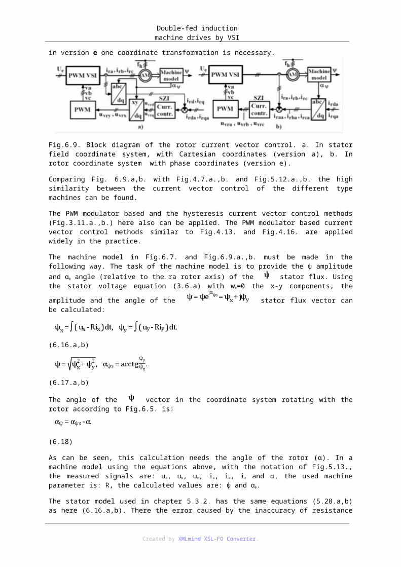
9. fejezet - Converter-fed synchronous motor driveThe circuit diagram of the converter-fed synchronous motor (CFSM) drive is given in Fig.9.1. Here all of the converters: the line-side ÁH, the motor-side ÁM and the excitation-side ÁG converter operate with line commutation. The line commutation of the thyristors in ÁM is possible, while the overexcited synchronous machine can provide the reactive power necessary for the commutation. In ÁM the commutations are done by the subtransient voltages of the SZ synchronous machine, that is why this commutation is called machine (load) commutation also. The supply is current-source-type, caused by the DC filter choke Le.
Fig.9.1. The power circuit of CFSM.
The converter ÁM can be controlled to rectifying and to inverter mode, so in spite of the unidirectional DC current mean value (Iek>0) the CFSM is capable of motor and generator mode operation. In motor mode ÁH is a rectifier, ÁM is an inverter, the mean value of the DC voltage is negative: U ek<0. In generator mode the converter modes are exchanged, consequently: Uek>0. Reversing the phase sequence of firing the thyristors of ÁM bidirectional rotation in driving and braking mode is possible (4/4 quadrant operation).
Fig.9.2. Block diagram of the controlled CFSM.
Fig.9.2. shows the block diagram of the flux and speed controlled CFSM. α h firing angle is the acting signal of the speed controller, αg firing angle is that of the flux (excitation) controller. Usually both controllers have subordinated current control loop. The α firing angle of ÁM is set by a self-controlled firing controller operated from signals of the synchronous machine SZ. By the self-controller the torque development can be optimized in motor (M) and generator (G) mode.
From the DC sides of converters ÁH and ÁG the self-controlled ÁM CFSM (the dotted-line surrounded part of Fig.9.2.) looks like a DC machine. In a real DC machine only ue and ug can be modified, the modification of the brush rocker position corresponding to the firing angle of the machine-side converter (α) is not used for this purpose. In a CFSM the excitation must be controlled always, because of the large armature reaction of the
Created by XMLmind XSL-FO Converter.

Converter-fed synchronous motor drive
synchronous machine.
Assuming ideal, zero resistance (Rr=0) rotor winding, for a given excitation current ig zero rotor voltage is
necessary: ūr=0. In this way in wk=w coordinate system the (3.6.c) rotor voltage equation is
the (3.6.d) rotor flux equation is . This is the principle of the so called flux constancy: the resistanceless short-circuited coil does not allow the variation of the flux linked with it. So in every operating point the subtransient flux vector linking with the rotor winding is constant. In stationary coordinate system (wk=0) the subtransient flux vector and the corresponding induced voltage vector are (assuming constant speed operating point: w=dαr/dt=const., αr is the angle of the rotor):
(9.1.a,b)
It means, that in steady-state both and ū” rotate with W=W1=2πf1 rotor/fundamental angular speed and their amplitudes (Ψ” and U”) are constant. Selecting t=0 instant to the positive maximum of ua”:
(9.2.a,b,c)
The stator voltage equation in stationary reference frame (3.6.a) considering (3.7) is:
(9.3)
Fig.9.3. Equivalent circuit of CFSM on the motor-side.
Using (9.3) the equivalent circuit of CFSM can be drawn (Fig.9.3). Comparing with Fig.2.7. high similarity can be found with R→Rt, L”→Lt, ua”→uta substitution.
In the ÁM motor-side converter according to the 6 thyristors the commutation frequency is variable: 6f 1 since the fundamental frequency is variable. Considering ideal thyristors, smooth DC current (i e=Ie) and R=0 stator resistance the classical line-commutated converter theory with overlap for steady-state can be applied (the overlap must be considered, since L” is much greater -with one order- than L t). This theory gives the following expressions for the DC voltage and current mean values:
(9.4.a,b)
Where . The α firing angle, the κ extinction angle (δ=κ-α is the overlap angle) and the μ=180o-κ commutation-reserve angle are related to the subtransient voltage. Fig.9.4.shows the vectors of the
Created by XMLmind XSL-FO Converter.
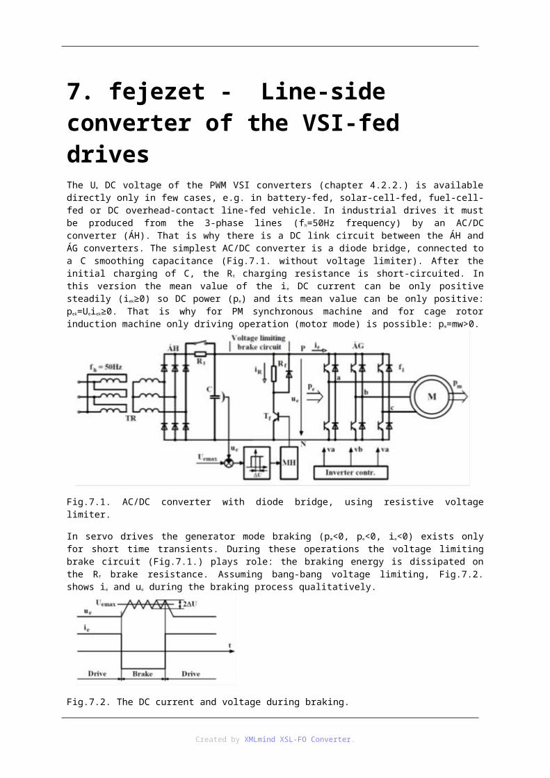
Converter-fed synchronous motor drive
terminal voltage (ū), the subtransient voltage (ū”) (9.2.b) and the current (ī) in inverter mode operation. The 60° sector started with the firing of the NC thyristor is drawn in bold. Using (9.3) (and approximation R=0) the derivative of the current vector (ī) is:
(9.5)
E.g. this is the speed of the current vector movement during the commutation NB→NC from point 1 to point 2. Considering the L”dī/dt vector movement speed, the control limits of the thyristor NC (B: firing ON limit (α=0º); K: extinction limit (µ=0º)) are marked on ū”. In generator/rectifier mode the drive can operate at the firing ON limit: α=αmin=0o also. In motor/inverter mode for the sake of safety the extinction limit (κ=κ max=180o) must not be reached, only maximum κmeg=160o extinction angle is allowed approximately.
Fig.9.4. Vector loci with ie=Ie and R=0 approximations.a. Voltage vectors, α=140o, δ=20o, κ=160o, μ=20o, b. Current vector.
In steady-state, neglecting the losses the Pmk mechanical power is equal to the mean values of the Pℓk air-gap power and the Pek DC link power (in motor/inverter mode: Pmk>0, Pek<0):
(9.6)
Using (9.4) and (9.6) the mean values of the speed and the torque can be expressed:
(9.7.a,b)
The maximal torque is developed by the CFSM at κmax=180o extinction limit in motor mode, and at αmin=0o firing ON limit in generator mode. Using (5.9, 5.10) the expression of the torque is:
(9.8.a,b,c)
According to (8.2.b) the amplitude of the fundamental current (I1) is proportional to the DC current (ie=Ie) with good approximation:
(9.9)
With given Ψ” and I1 the maximal Mk is at ϑ1=±90o torque angle. Fig.9.5. shows Mk/Mn relative torque (referred
to Mn=(3/2)ΨnIn nominal torque) vs. I1/In I≌ e/Ien (where ). Besides the machine (load)
Created by XMLmind XSL-FO Converter.

Converter-fed synchronous motor drive
commutation operation limits of ÁM (αmin=0o-os and κmax=180o) the safe motor/inverter mode limit curve is also drawn (κmeg=160o extinction angle). It can be established, that similarly to the separately excited DC machine the torque is proportional to the DC current. In motor mode: Mk=KMIe, in generator mode: Mk=KGIe, KM>0, KG<0. In the shaded areas the drive can operate only with forced commutation (VSI or CSI supply). A given M k torque should be developed with the possibly minimal I1 current. For the CFSM it requires a two-stage self controlled firing controller, which provides κ=κmeg operation in motor/inverter mode, and α=αmin operation in generator/rectifier mode. In practice the controls from the position of the shaft (α) or from the position of the
subtransient flux vector (αψ”) are used. The former is called: firing control from the shaft, the later: firing control from the flux.
Fig.9.5. The mean value of the torque vs. the fundamental current.
The firing controller from the subtransient flux vector results in field-oriented firing control. Fig.9.6.a. presents the block diagram, Fig.9.6.b. shows the firing levels (for w>0 and a,b,c phase sequence). The
flux vector is provided by stator machine model (detailed in Fig.5.14), the α ψ” angle and the ψ” amplitude are provided by the blocks ARC and AMPL respectively. The M/G motor/generator two-stage signal changes the comparing levels according to the κmeg and αmin operation modes. In motor mode to the κ=κmeg=const. extinction angle a operation point dependent firing angle is corresponding (α=κmeg-δ). Therefore in this case the Δ signal of the FG function generator corrects the firing comparing levels using the load dependant input value I e
(in field-weakening more accurately Ie/ψ”). The firing control from the subtransient flux vector
is identical with the firing control from the subtransient voltage vector, since e.g. at w>0: αu”=αψ”+90°.
Fig.9.6. Firing control from the subtransient flux vector. a. Block diagram, b. Firing levels for w>0.
More practical to fire from , since it moves on a more smooth path than the voltage vector, and its amplitude in the normal range is constant, while the amplitude of ū ” is proportional to w. The firing from the shaft position (α) has larger load dependency in motor/inverter mode, and Δ correction is necessary in generator/rectifier mode also.
Created by XMLmind XSL-FO Converter.

Converter-fed synchronous motor drive
Fig.9.7. Machine commutation current vector loci (w>0). a. Generator/rectifier mode: α=20°, δ=20°, b. Motor/inverter mode: α=140°, δ=20°, κ=160°.
Fig.9.7. shows the current vector loci in coordinate system fixed to the flux vector (field coordinate system) with field-oriented firing control and machine commutation, assuming smooth DC current (i e=Ie). The marked amplitudes and angles come from Fig.9.4.; Fig.9.4.a. and Fig.9.7.b. correspond to operation point with κ=κmeg=160° and approx. nominal motor mode I1 current. In this case approx. ϑ1=120° can be reached as best torque angle.
It can be proved, that in the range R>WL” the safe machine commutation is not possible. The border angular speed is:
(9.10)
With the usual machine parameter it is reached at f 1h 5Hz. In the W<W≌ h, f1<f1h range step commutation is used. Since in this case fh/f1>50 Hz/5 Hz=10, so there are at least 10 firings in ÁH between two firings of ÁG. Consequently in this case the commutation can be done by ÁH, by controlling the current vector to zero in every 1/6th machine period (Fig.9.8.a.). The step commutation using the ī=0 current vector can be made faster, if during the commutation the TE thyristor connected parallel with L e (Fig.9.1.) is fired ON. Therefore the current flowing in Le can remain unchanged (ie=Ie) during the commutation, only the motor current must be reduced to zero, and then must be increased back to Ie. There is not a limit for the phase angle of Ī1 in step mode, so the torque angle in motor mode can be ϑ1=90°, in generator mode ϑ1=270°(-90°) also (Fig.9.8.b.,c).
Created by XMLmind XSL-FO Converter.

Converter-fed synchronous motor drive
Fig.9.8. Step commutation current vector loci (w>0). a. In stationary coordinate system, b.,c. In field coordinate system in generator and motor mode.
In the range W>Wn, f1>f1n field weakening must be applied. In this case the amplitude of the subtransient flux vector must be controlled in the following way approximately:
(9.11)
Fig.9.9. presents the possibly covered operation range, assuming 4/4 quadrant and field weakening operation on the W(Mk) plane. In the step commutation range there is not continuous operation usually.
Fig.9.9. Operation ranges extended by the field weakening on the W(Mk) plane.
Let’s mention, that the largest variable speed drive in the word is a CFSM. This 101MW drive is used for a fan of a wind tunnel of the NASA. This huge wind tunnel is used for aerodynamic investigations of supersonic aircrafts.
If a cage rotor induction machine is made resultantly capacitive by parallel capacitors (Fig.8.7) it is also capable of operating from line commutated converter (Fig.9.1.). This so called capacitively compensated converter-fed induction machine is capable of operating in narrow frequency range only, that is why it is rarely used only.
Created by XMLmind XSL-FO Converter.

10. fejezet - Switched reluctance motor driveIn the switched reluctance motor (SRM) both the stator and the rotor are cogged. The number of cogs on the wounded stator is Z=2pm*, the number of cogs on the non-wounded rotor is usually Zr=Z±2p (2p is the number of poles, m* is the number of the phases). In the machine in Fig.10.1. these values are: m*=3, 2p=2, Z=6 and Zr=4. Only the coils of phase a are drawn in the figure. The most commonly applied SRMs have m *=3 and 4 phases.
Fig.10.1. Switched reluctance motor, m*=3, 2p=2, Z=6, Zr=4.
Using the energy theorem (calculating the energy modification for Δt time interval) the torque can be expressed. The result is simple, if at a given time current flows only in one phase, the saturation is neglected and only the cupper looses are considered. In this case the torque developed by the ith phase is:
(10.1)
Where ii is the current of the ith phase, L i is its self-inductance, α is the angle of rotation of the rotor. According to this expression, the torque is independent of the current direction (that is why the power circuit capable of one current direction in Fig.10.1. is enough in each phase), and the torque exists only if dL i/dα≠0. If the mutual inductances can be neglected comparing with the L i self-inductances of the phases (it is usually a good approximation), then more phases can conduct simultaneously. In this case the resultant torque is
(10.2)
Fig.10.2. Trapezoidally changing Li self-inductance and the corresponding dLi/dα factor.
The factor dLi/dα is determined by the motor, the value is determined by the supply. The self-inductance of the phases (Li) depends on the α and changing periodically with Zrα=2π periodicity, repeated Zr times in one revolution. Assuming trapezoidal inductance change, Fig.10.2. shows the inductance of the ith phase L i(α) and its dLi/dα factor.
The larger the Lmax-Lmin difference, the larger the dLi/dα factor and the torque which can be developed with a
Created by XMLmind XSL-FO Converter.

Switched reluctance motor drive
given current. Positive torque (mi>0) can be developed by current flowing during dL i/dα>0 section, negative torque (mi<0) can be developed by current flowing during dL i/dα<0 section. Both sections have β length. At dLi/dα=0 sections current flow is useless, since it does not develop torque, only losses would be generated. Accordingly, the phase currents must be synchronised to the rotor position (α).
The phase currents must be fitted to the motor according to the drive demand. That is why the SRM drives are designed and manufactured in complex way. The smooth, pulsation free torque is frequently a demand (e.g. in servo and vehicle drives). Fig.10.3. presents the fitted supply to develop smooth torque for three-phase machine with trapezoidal phase self-inductances La(α), Lb(α) and Lc(α). In this case the condition of the fitted supply is the given length of the torque development sections: β>360°/3=120°. According to Fig.10.3.b.,c.,d. the rectangular shape βi=120° wide current pulses in these sections provide the ideal fitted supply. The solid line current curves develop positive torque (m>0), the dotted ones negative torque (m<0). The currents to develop positive and negative torque have the same direction, but shifted by δ≈180° from each other. In the real case the phase currents can not be increased and decreased instantaneously because of the self-inductances. Consequently the shape of the phase currents is significantly modified at high speed.
Fig.10.3. Fitted supply of a three-phase, trapezoidal self-inductance SRM. a. Phase self-inductances, b.,c.,d. Fitted phase currents, e. Torques.
The best utilization of the trapezoidal self-inductance SRM is got if the width of the current flow is equal to β (βi=β). However in this case (except at βi=120°) the torque is pulsating with 6nZr frequency (n is the rotation speed).
If the three-phase machine is star-connected, applying the connection in Fig.10.1. for three-phase, the simple power electronic circuit in Fig.10.4 can be got. Assuming ideal semiconductors, it can switch +U e, -Ue and 0 voltages to the phases. Switching between these three values with high frequency (PWM) the phase currents can be controlled. Since only positive phase currents are necessary, in unipolar mode +Ue and 0, in bipolar mode +Ue
and -Ue are switched. The mean value of the ie DC current is positive in motor mode (I ek>0) and negative in generator mode (Iek<0). Assuming lossless power electronics and motor the power mean values are: Pmk=MkW=Pek=UeIek. The constant DC voltage (Ue≈const.) is provided by an AC/DC converter presented in Fig.7.1. if generator (brake) mode occurs only during transients.
Fig.10.4. Three-phase star connected SRM with power electronics.
Created by XMLmind XSL-FO Converter.

Switched reluctance motor drive
Fig.10.5. presents the block-scheme of a speed controlled three-phase SRM drive. The SZW speed controller provides the torque reference ma. The squareroot of its absolute value │ma│ (by NG) is proportional to the phase current amplitude:
(10.3)
According to (10.2) the NG squareroot block linearizes the torque control loop (it is reduced to current control). The phase current references (iaa, iba, ica) correspond to the fitted supply (to Fig.10.3).
Fig.10.5. Block-scheme of a speed controlled three-phase SRM drive.
The synchronisation to the rotor position is done by the FGA, FGB, FGC function generators, using Z rα’. If w>0 and ma>0, then the operation is in motor mode: Z rα’=Zrα. If w>0 and ma<0, then the operation is in generator mode: Zrα’=Zrα-δ. The phase current amplitudes are set by the × multiplication, using I a. The PWM current controllers per phase can be implemented by PWM controllers or by hysteresis controllers. The control signals va, vb, vc switch the transistors TA, TB, TC (Fig.10.4.), the control signal vo switches transistor T0. In practice, the PWM is implemented by T0.
In a real case the step change of the phase currents is not possible because of the inductances. It can be compensated by a speed dependent pre-firing. The PWM operation is possible until such speed and torque, where the on-section of the +Ue voltage is long enough to develop the phase current with amplitude Ia. Beyond this a so called single pulse operation is possible. In this range the torque is pulsating and the torque loadability decreases.
Obviously the smooth, pulsation free torque operation can be implemented not only with trapezoidal phase self-inductances. The shape of the fitted phase currents i i(α) can be determined by the expression (10.2) always. To do it, the machine characteristic self-inductance angle dependency per-phase Li(α) must be known.
Created by XMLmind XSL-FO Converter.

11. fejezet - Speed and position controlAmong the task specific controls the speed and the position controls are discussed.
1. Speed controlThe speed control can be drive specific also. The speed signal of a DC machine can be provided by a machine model using (1.1.a and 1.2.a):
(11.1)
The combined machine model of the cage rotor IM (Fig.5.15.) can provide the w speed signal also (5.34). If these calculated w speed signals are used as feed-back signal of the speed controller, then the speed control is drive specific, so called sensorless type.
In the next coming investigations the speed feed-back signal is provided by a speed sensor. According to Fig.1.3. there is a subordinated torque loop to the speed controller. However the torque control in the investigated drives can be reduced to current/current-component control. Accordingly, current/current-component control is subordinated to the speed control in practice.
In this chapter the speed control of a 4/4 quadrant PWM chopper-fed DC drive with subordinated current control is investigated as an example. Its block-scheme is presented in Fig.11.1. According to the subordinated structure the reference value of the SZI current controller (i’ a) is set by the SZW speed controller. In the dotted-line surrounded control loop the signals with prime have [V] dimension in analogue implementation, and dimensionless in digital implementation. Avw, Avi and Au are the transfer factors of the speed sensor, the current sensor and the PWM DC chopper (Fig.1.21.) respectively.
Fig.11.1. Block-scheme of the speed controlled DC drive.
The controller SZW can operate in the saturated and in the linear range.
The saturated range is realized, if the speed has such a value, which results in SZW output i’ a reaching the limit (saturated) value (+I’korl or -I’korl). (SZI is in saturation, if its output is at ±U’ vm value.) These correspond to the allowed current limit for the motor and the chopper (±I’korl). The current limitation provides protection functions. In the investigation of the saturated operation of the speed controller it is assumed, that i’ a=±I’korl and the time function of i’k(t) from I0 approaches I’korl with Ti time constant:
(11.2)
I.e. the inner current control loop is in linear range described by (2.24).
At start up: I0=0. Current i’k(t) reaches I’korl value in approx. 3Ti, then while i’a=I’korl the motor accelerates with
Created by XMLmind XSL-FO Converter.

Speed and position control
maximal current (i’k=±I’korl) and maximal torque (mk=Mkorl=kϕIkorl). The time function of the speed can be calculated from the following differential equation:
(11.3)
Meanwhile the speed controller has not any effect. The acceleration rate depend on m t and θ. The current limitation periods can be avoided by limiting the gradient of the speed reference (ramping, Fig.11.2.). The drive can track such a speed reference (wa), for which the following condition is true:
(11.4)
Fig.11.2. Gradient limited speed reference (wak).
The speed and current tracking properties of the controller operating in linear range are determined by both controllers. First the current controller, then the speed controller should be tuned.
The linear and saturated operation of the SZW speed controller is presented in Fig.11.3 by its typical transient response to wa step change in the reference.
1. Section I (saturated): the speed curve corresponds to (11.3), ik=Ikorl. Controller SZW comes out the saturation at speed error Δw*.
2. Section II (linear): depending on the structure and setting of the controller, the speed reaches the reference, and the current its stationer value (iks) with or without oscillation, with or without error. iks can be calculated from the necessary torque mks=mts to maintain the steady-sate value of the speed (w=wa): iks=mts/(kϕ).
3. Section III: it is again saturated: i’a=-I’korl.
4. Section IV: it is linear, stationary state, with mt=0 load torque.
Fig.11.3. Typical transient responses to step change of the speed reference.
To design the speed control in the linear range, the symmetrical optimum method is widely used. Let’s
assume, that the transfer function of the subordinated current control loop has been adjusted to
(2.24). Since i’a=Aviia so . To determine the setting of the speed controller, the simplified block scheme in Fig.11.4. is used.
Created by XMLmind XSL-FO Converter.

Speed and position control
Fig.11.4. The simplified block scheme of the speed control loop. a. With the physical signals of the motor., b. With signals normalized to voltage dimension.
Fig.11.4.a. can be derived from Fig.11.1. by neglecting the effect of the speed change (kϕw) to the current control. The surrounded part is the drive specific part. In Fig.11.4.b. voltage dimension signals are used using Fig. 1.4. The transfer function of the open speed control loop using Fig.11.4.b. is:
(11.5)
Where T=CTm is a resultant time constant, C=(kϕ/R)(Avi/Avw)is a dimensionless value. The transfer function of the PI type SZW speed controller is:
(11.6.a,b)
Substituting s→jω, the Bode diagram of the Y(jω) frequency-function is given in Fig.11.5. According to the practice: Ti<<T. The crossover angular frequency (ωcw) and the cut-off angular frequency (1/Tw) can be modified by the speed controller (by YF(jω)). The design of the controller based on selecting Ti<Tw=BTi<T, so inserting a -20 dB/decade slope section between the -40 dB/decade slope sections.
Fig.11.5. The frequency diagram of the open speed control loop.
The cutoff frequency is set by KF to get ωcw at the middle of the -20 dB/decade slope section. It can be proved, that in this case at ωcw the phase lag φ=arc(Yw, Δ w) is minimal (the phase margin φt is maximal), i.e. the system is the best considering the stability. For this case using Fig.11.5. the following expression can be written:
Created by XMLmind XSL-FO Converter.

Speed and position control
. Using│Y(jωcw)│=1, the setting rules for the parameters of the speed controller are:
(11.7.a,b)
The coefficient B is selected using simulations, depending on the desired tracking property. Its optimal value for reference step is B≈10, for load step is B≈5 (fast, small overshoot tracking). Proper behaviour for both cases can be got at B≈7.5. It can be established, that the faster the current control loop (the smaller the time constant T i), the larger parameter KF and the smaller parameter TF can be selected, i.e. the faster the speed control will be.
2. Position controlIt is used in servo drives most commonly. Its basic types are:
1. PTP point to point control, (e.g. spot welder robot),
2. CP continuous path, path tracking control (e.g. arc welder robot).
The scheme of the subordinated structure position control is presented in Fig.11.6. (the position is represented by the α angle of the motor shaft). The inner speed control loop coincides with Fig.11.1. The w’ a speed reference is set by the SZP position controller. Avp is the transfer factor of the position sensor.
Fig.11.6. Block scheme of the position control.
The behaviour of the position control is investigated in detail for the PTP control, in that case when the speed reference is limited to ±W’poz (Fig.11.6) (Wpoz is usually less than Wmax allowed for the drive). The transient response functions of the system for an αa magnitude step change in the position reference are given in Fig.11.7. Such a large reference step is considered, which results in limited (saturated) operation of the SZP, SZW and SZI controllers. The saturated operation of the SZP, SZW and SZI controllers mean, that their outputs are limited to±W’poz, ±I’korl and ±U’vm values respectively. The reason of the saturated operation is the high and/or long-lasting error on the input of the controllers.
Created by XMLmind XSL-FO Converter.

Speed and position control
Fig.11.7. Typical transient response functions for position reference step.
1. In sections I, II (acceleration and constant speed operation): SZP is saturated, w a=Wpoz. SZW is saturated in section I, and linear in section II. SZP comes out the saturation at Δα2 position error.
2. In sections III, IV (deceleration and positioning): SZP is in linear mode, wa<Wpoz. In section III (current limited section) SZW is saturated. In section IV every controller is in linear mode. The optimal design of SZP can be determined in this section.
For small αa reference step the sections II and III can be missing.
The simplified block scheme of the position control loop for the linear section IV is shown in Fig.11.8. Here
represents the speed controlled drive (Fig.11.1.). is the transfer function of the closed speed control loop.
Fig.11.8. The simplified block scheme of the position control loop.
The transfer function of the SZP position controller is usually PID type:
(11.8)
The transfer function of the open position control loop is:
(11.9)
(11.10.a,b,c)
It can be established, that the natural α=∫wdt integration effect (1/s) results in modified effects of the position controller’s PID parameters. E.g. the D parameter (Tpd) affects the loop gain (K1), the P parameter (Kp) affects the integration time (T1). In the practice, for PTP control P and PD position controllers are applied. By these controllers “type 1” position control loop can be implemented, i.e. for position reference step the tracking is errorless in steady-state.
Position control with proportional (P type) controller.
In this case Yp=Kp, the transfer function of the open position control loop is:
(11.11.a,b)
Assuming PI type speed controller, Fig.11.9. presents the Bode diagram of the open position control loop (s→jω). As can be seen, in the ω<ωcw frequency range: , so in this range│Yα,Δα│=│1/(jωT)│.
The phase shift of the open position control loop ( ) is independent of Kp. Modifying Kp, │Yα,Δα│ can be shifted up and down. Increasing Kp, the crossover frequency of the position control loop (ωcp=1/T=Ap) getting closer to the crossover frequency of the speed control loop (ωcw). The maximal value of Kp
is determined by the phase margin (φt):
Created by XMLmind XSL-FO Converter.
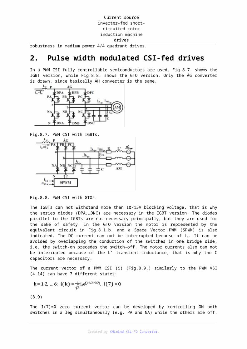
Speed and position control
(11.12)
where are the angles of the frequency functions. To get acceptable control behaviour for the position control loop, φ t≥45° phase margin is required. This requirement determines the maximal value of Kp and Ap, and the minimal value of T. It can be established, that the faster the speed control loop (the larger ωcw), the larger crossover frequency/loop-gain (ωcp=Ap), the smaller the time constant T=1/ωcp and the faster the positioning can be.
Fig.11.9. The frequency diagram of the P type open position control loop.
This rule can be generalised: fast speed control needs fast current control, fast position control needs fast speed control. I.e. in a subordinated control structure the speed of the inner control loop limits the speed of the outer control loop.
If ωcw>>ωcp (if φt≥60°), then approximately. Considering it in (11.11.a), the transfer function of the closed position control loop is:
(11.13)
Consequently the controlled α position tracks the αa reference with lag T:
(11.14.a)
(11.14.b)
The later expression of the Δα position error (11.14.b) is valid if αa=const. Then Δα and w change exponentially:
(11.15.a,b)
(11.16)
With the Δα0/T=ApΔα0=Wpoz expression it is assumed, that the section III (current limited deceleration) misses. The torque by (1.a) motion equation and mt=0 assumption is:
Created by XMLmind XSL-FO Converter.
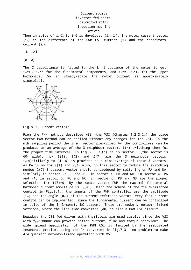
Speed and position control
(11.17)
Because of the missing section III the inequality θWpoz/T<Mkorl=kϕIkorl must be fulfilled. It determines a minimum value for T and a maximum value for Ap.
Fig.11.10. Time functions in the section IV (positioning).a. Speed, b. Position, c. Torque (mt=0).
The exponential tracking (solid curves in Fig.11.10.) is overshoot free, but slow.
A finite time (Tf) linear tracking can be reached by constant deceleration (dw/dt=-Wpoz/Tf) braking. Here the time functions for 0≤t≤Tf, with mt=0 are the following:
(11.18.a)
(11.18.b)
(11.18.c)
Now the θWpoz/Tf<Mkorl condition must be satisfied. At the exponential tracking: Δαo=WpozT, at the linear tracking: Δαo=WpozTf/2. Consequently: Tf=2T. The time functions of the linear tracking are given in dotted lines in Fig.11.10. From (11.15, 11.16) and (11.18.a,b) it is clear, that the positioning speed at the exponential tracking is
proportional to Δα, at the linear tracking to :
(11.19.a,b)
Created by XMLmind XSL-FO Converter.

Speed and position control
(11.20.a,b)
At the linear tracking for ± signed Δα the next expression is valid:
(11.21)
At the linear tracking the position controller is P type also, but Kp and Ap (11.11.b) are not constant, they depend on Δα, i.e. SZP is a nonlinear variable gain controller.
Fig.11.11. shows the w(Δα) (in section II and IV the wa(Δα)) function for such a positioning process, where the section III is missing and mt=0. Difference between the exponential and linear tracking can be identified only in section IV. The initial position error for the exponential tracking is Δα o>Δ, not to get current limit. (Δ is the rotation angle in section I, in the section with current limit). At linear tracking the gradient of the w(Δα) parabola is:
(11.22)
Its value at the origin would be ∞. Because of stability problems, near the origin the exponential tracking should be followed in this case also, with a Apmax>>Ap parameter setting.
Fig.11.11. The w speed vs. the Δα position.
Only the basic principles of the speed and position control are described in this subject. In both cases other control methods can be used, too: sliding-mode control, model reference control, fuzzy control, neural network based control, etc.
Created by XMLmind XSL-FO Converter.

12. fejezet - ApplicationsThe modern practical applications of the VSI-fed drives and the CFSM drive are described in this chapter.
1. Flywheel energy storage driveOne possible way of electric energy storage is the flywheel electrical drive, which stores the energy in kinetic form.
The flywheel storage uses the EL kinetic energy of a mass with qL inertia rotating with wL angular speed. The maximal kinetic energy corresponds to the maximal speed:
(12.1)
If the kth part of the ELmax energy should be utilised, then:
(12.2)
(12.3)
Usual practical values are: k=0.75, wLmin=0.5wLmax.
Fig.12.1. Modern flywheel drive. a. Block scheme, b. Operation range.
Fig.12.1. Modern flywheel drive. c. Fully utilising the limits.
The kinetic energy can be modified by the mL torque of the flywheel’s drive, i.e. by its pL power:
(12.4)
During deceleration (decreasing wL, discharging) energy is withdrawn, during acceleration (increasing wL, charging) energy is supplied to the flywheel. In a modern flywheel drive (Fig.12.1.a.) L is the flywheel, Á is the gearbox, VG is the electrical driving machine, TE is the power electronic circuit, H is the electric grid, q L is the resultant inertia referred to the shaft of the flywheel. The VG, TE and H units must be capable of bidirectional
Created by XMLmind XSL-FO Converter.

Applications
power flow. The VG electric machine is in motor mode at p L>0 (charging), and in generator mode at pL<0 (discharging). The modern, low-loss applications are gearless, they use direct drive.
The usual operation range of the TE-VG electric drive is given in Fig.12.1.b. on the wL-mL plane. In the wLmin£ωL£wLmax operation range the maximal power is +PLmax at charging and –;PLmax at discharging. The maximal driving torque of the drive is MLmax=PLmax/ωLmin, the maximal brake torque is –MLmax. It can be established, that the flywheel drive is a mono-directional two quadrant drive, and its normal operation range is the field weakening. The nominal point of the drive should be selected to point 2: MLn=MLmax, wLn=wLmin and PLn=MLnwLn=PLmax. Fig.2.1.c. shows that case, when the limits are fully used, when the pL power pulsates in the range ±PLmax with 2DT periodicity and the energy is changing between ELmin and ELmax linearly. It can be derived for DT:
(12.5.a,b)
Where TLin is the nominal stating time of the drive.
The principal task of the flywheel drive is to compensate (smooth) the pulsating electric power. The control of the cage rotor induction machine (Fig.7.7) driven flywheel drive is described as an example. One possible block scheme of the control loop to compensate the power pulsation is presented in Fig.12.2.
Fig.12.2. The block scheme of the control loop of the cage rotor induction machine driven flywheel drive connected to the three-phase grid.
The pulsating power of the G consumer or generator should be compensated. From the measured pG
instantaneous value the SZ filter provides the mean value (pGk) and the difference of these two powers sets the electric power reference of the flywheel drive (pLGa):
(12.6)
From pLGa and wL unit MA provides a torque reference:
(12.7.a)
(12.7.b)
Where pLGa-pLv is the mechanical power of the drive, pLv is the wL dependent loss of the drive, mLv=pLv/ωL is the corresponding torque. The mLv motor mode torque is necessary to keep the wL angular speed constant. Instead of the MA torque set point element power controller also can be used, but the power of the flywheel drive (p L) must be measured too in this case. From the wL and mLa signals the FA block provides the rotor flux reference of AL machine. It mainly depends on the speed:
Created by XMLmind XSL-FO Converter.

Applications
(12.8)
Where Yrn is the nominal rotor flux. The machine-side SZÁLG current vector controller controls the torque and the flux of the AL induction machine by the ÁLG converter. The control can be implemented by field-orineted control (see chapter 5.3.1.). From the flux reference (yLa) and the torque reference (mLa) the current components references can be calculated in the field reference frame:
(12.9)
These are constrained by the SZÁLG current vector controller.
The grid-side voltage controller (SZULE) controls the DC voltage (uLe) by its active power reference (pLHa). The reference of the reactive power (qLHa) is determined by external grid demands. The SZÁLH current vector controller controls the active and reactive power of the flywheel drive by the ÁLH converter. The line-oriented current vector control can be implemented according to chapter 7.1.1. From the active and reactive power references (pLHa and qLHa) the current components references can be calculated:
(12.10)
These are constrained by the SZÁLH current vector controller.
The structure of a permanent magnet synchronous machine driven flywheel drive is similar. The block scheme of the double-fed induction machine driven flywheel drive is different because of the missing field weakening possibility.
The block scheme of the control (Fig.12.2.) does not contain the initial charging part (the starting and acceleration form zero speed).
As an example, the compensation of a sinusoidally pulsating pG power is demonstrated in Fig.12.3. in per-unit system. The amplitude of the pulsation is set to such a value for k=0.75, which results in reaching the speed (wLmin and wLmax) and power (±PLmax) limits. At the beginning of the power pulsation compensation the speed of the flywheel is set to such a value, which results in symmetrical compensation reserve. The corresponding values are (wLn=wLmin):
(12.11)
For k=0.75: , ELk=2,5ELmin, ELmax=4ELmin.
Fig.12.3. Perfect compensation with reaching the speed and power limits. a. The current vector of the AL
Created by XMLmind XSL-FO Converter.

Applications
induction machine in field reference frame.
Fig.12.3. Perfect compensation with reaching the speed and power limits. b. The torque and speed of AL.
Fig.12.3. Perfect compensation with reaching the speed and power limits. c. The power of the flywheel drive (pL) and the resultant power (pG+pL).
Fig.12.3. Perfect compensation with reaching the speed and power limits. d. The magnitude of the rotor flux vector in AL.
Fig.12.3. Perfect compensation with reaching the speed and power limits. e. The compensation process on the ωL-mL plane.
The example drive can not compensate perfectly larger amplitude or larger period power pulsation.
Created by XMLmind XSL-FO Converter.

Applications
Among the practical implementations, the product of Beacon Power can be mentioned (Smart Energy 25). In this product the flywheel is driven by permanent magnet synchronous machine, it rotates in vacuum with magnetically levitated bearing, with 8000-16000rpm (k=0,75). It can provide PLmax=100kW power for 15min, i.e. ELmax-ELmin=25kWh.
2. Electrical drives of vehiclesAs examples, among the railway traction drives a modern locomotive, among the urban transportation drives a modern VSI-IM trolleybus drive are described.
2.1. LocomotiveIt is single-phase (50Hz, 25kV) DC-link VSI-fed vehicle (Taurus locomotive). Five power components can be distinguished: line transformer, line-side converters, the DC link, the motor-side converters and the induction machines (Fig.12.4.).
Fig.12.4. The power circuit of the VSI-IM driven locomotive.
The figure presents in detail the circuit of one double-machine driven bogie. Every machine has own inverter. Consequently the inverters and motors can be controlled independently, so e.g. the adhering force can be utilised better. Every bogie has a power electronic unit. It contains three parallel connected line-side 4QS (Four Quadrant System) two-level converters (ÁH1, ÁH2, ÁH3) and two two-level VSIs (INV1, INV2). This configuration makes possible to use exactly the same type GTO legs in the line-side converters (ÁHx) and in the inverters (INVx). Such configuration is used for high power locomotives (e.g. 4·1600kW=6400kW).
The 4QS four-quadrant line-side converters make possible the regenerative electrical brake operation, and the currents in the input contact wire are sinusoidal with cosj=±1 power factor. The 4QS converters are controlled by active power control subordinated to DC voltage control. Since the single-phase power pulsates with 2fh=100Hz frequency, there is a filter (L1,C1) in the DC link tuned to 100Hz.
The principle of the control of the VSI-fed vehicle drive is the field-oriented current vector (chapter 5.3.). Until the load makes possible, constant torque angle (ϑ1) control (constant fr rotor frequency control) is used, resulting in energy saving operation. The regions of the control are presented in Fig.12.5. for motor operation. In Fig.12.5.a. the Ī1 current vector in d-q reference frame is given, in Fig.12.5.b. the torque is given in the M-w 1
plane with the regions and the limits.
Created by XMLmind XSL-FO Converter.

Applications
Fig.12.5. Control regions for steady-state motor mode operation. a. Ī 1 current vector in d-q- reference frame, b. Limits on the M-w1 plane.
Region I.: Energy saving operation, the torque angle is: ϑ1=ϑ1opt=ϑ1n, the torque is (M≤Mn):
(12.12)
Region II.: Nominal rotor flux operation (Yr1=Yr1n), w1£w1n=2pf1n, M³Mn, the torque is:
(12.13)
The maximal torque (Mmax) is determined by the current limit (I1max).
Region III.: Field weakening operation, w1>w1n, the flux and the torque are:
(12.14.a,b)
(12.15)
For regenerative brake operation the Fig.12.5. should be reflected to the horizontal axis.
The locomotives have torque (traction force) control, subordinated to speed control (Fig.12.6.). In forward and reverse running the torques have opposite sign, the sign inverting is done by block E/H. During starting the vehicle accelerates till the va speed set by the driver, with traction force settable by the limit torque mkorl (in the w1>w1n speed range the KORL block can decrease the m korl value set by the driver). Reaching the v a speed the SZV speed controller sets the torque reference necessary to keep the required speed. Instead of torque limitation, acceleration control is also an option.
Fig.12.6. Block scheme of the speed control with torque limitation.
Created by XMLmind XSL-FO Converter.

Applications
2.2. TrolleybusThe operation of the urban transportation vehicles between two stops contains acceleration, coasting and deceleration (braking). The motor develops tracking/braking force only during the acceleration and braking. Therefore speed control is not applied in these vehicles, only the acceleration and deceleration process are controlled usually by the torque.
Because of the frequent starting and braking processes, with lossless starting and regenerative braking significant energy can be saved. By regenerative braking, according to the measurements in normal traffic conditions the 30-35% of the supply energy can be supplied back.
The main power circuit of a VSI-IM trolleybus drive is given in Fig.12.7.
Fig.12.7. VSI-IM trolleybus drive.
The AM induction motor is connected to the UT DC supply through an IGBT two-level voltage source inverter (INV). The UT supply should be provided by the circuit given in the figure, since the trolleys of the vehicle can connect shortly opposite polarity voltage to the vehicle in the cross roads. It is rectified by the D1-D4 diode bridge. At normal polarity the regenerative braking is possible through IGBTs T1, T2. Smoothing of U T voltage is done by filter Lsz-Csz, the initial charging of Csz is done by the KT, RT charging circuit. There is a TL surge absorber, KF1, KF2 main contactor and a noise filter on the supply side.
The controlled motor operation and the controlled regenerative braking can be implemented by the control of the inverter. The condition of the regenerative braking is that the supply voltage should stay bellow the allowed UT £UTm. If during regenerative braking the opposite energy flow causes reaching U Tm value, then the TF transistor can connect resistance RF parallel to Csz. With ON-OFF switching the resistance RF the UT voltage can be controlled.
The basic principle of the control of the VSI-fed trolleybus drive is the field-oriented current vector control, but here only the acceleration and the braking is controlled. The different control regions for motor/acceleration mode are shown in Fig. 12.8.: Fig.12.8.a. presents the Ī1 current vector in d-q reference frame, Fig.12.8.b. shows the torque on the M-w1 plane with the regions and the limit curves. Opposite to the railway VSI drive (Fig.12.5.) there are only two regions here, since the constant speed energy saving operation is not necessary in the urban transportation.
Created by XMLmind XSL-FO Converter.

Applications
Fig.12.8. Control regions for VSI-fed motor mode operation. a. Ī1 current vector in d-q reference frame, b. The limits on the M-w1 plane.
Region I.: Nominal flux operation: Yr1=Yr1n, w1£w1n. The torque can be calculated by (12.13), Mmax is determined by the I1max current limit.
Region II.: Field weakening operation, w1>w1n, the flux can be calculated by (12.14), the torque by (12.15).
For regenerative brake operation the Fig.12.8. should be reflected to the horizontal axis. The generator mode current limit I1max is usually less, than in motor mode.
Basically the trolleybus has torque (traction force) control (Fig.12.9).
Fig.12.9. Block scheme of a torque controlled drive.
The driver sets the ma torque reference by the GY acceleration pedal for starting/acceleration and by the F brake pedal for stop/braking. The torque reference is positive for acceleration and negative for braking in forward running.
3. Wind turbine generatorsThe wind power plant contains the generator, the wind turbine, the mechanical gearbox, the power electronic circuit, the control system and the auxiliary equipments. The modern wind turbine generators are VSI-fed induction or synchronous machine drives operating in generator mode.
Created by XMLmind XSL-FO Converter.
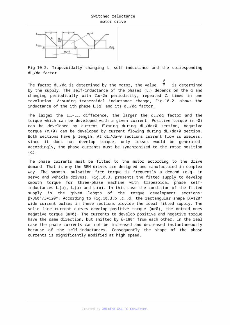
Applications
Fig.12.10. Characteristics of the wind turbine. a. Power-wind speed curve, b. Torque-angular speed curve.
The characteristic PT(v) power-wind speed diagram and the M(W) torque-angular speed (on the shaft of the turbine) diagram are given in Fig.12.10a. and b. respectively. At the region A-B where the wind speed is v0£v£vN
(this is the optimal pitch angle region) the power factor (aerodynamic efficiency) of the wind turbine (12.16) is optimal (maximal):
(12.16)
PT=MTWT=MW is the power of the wind turbine, PSZ is the power of the wind rotating the wind turbine. In this region the angular speed of the wind turbine WT (the angular speed of the generator W) must be controlled approximately proportionally to the v wind speed to get maximal power factor C Pmax between point A and B. At the nominal wind speed (vN) in point B the power of the wind turbine is (neglecting the losses):
(12.17)
In the region A-B the power PT and torque M are approximately:
(12.18.a,b)
In region B-C (vN£v£vmax) constant PTN nominal power should be provided by the limitation/control of the power at the wind turbine and at the generator.
The basic aim of the control in both regions to utilise the wind turbine power (limited to P TN) as much as possible. At a given v wind speed the PT power can be controlled at the wind turbine by turning the nacelle relatively to the direction of the wind and by turning the blade around its longitudinal axis (b angle pitch control), at the generator by the control of the angular speed. The limitation of the power is done at the wind turbine.
Nowadays the direct driven synchronous machine and double-fed induction machine are applied as generators most frequently. The block schemes of the permanent magnet synchronous machine (PMSM) and the double-fed induction machine (DFIM) wind turbine generators are given in Fig.12.11. and Fig.12.12. respectively.
Created by XMLmind XSL-FO Converter.

Applications
Fig.12.11. Block scheme of the direct driven PMSM wind turbine generator.
The central controller (KSZV) determines the speed reference (wa) of the generator and the pitch angle reference (ba) using the wind speed (v) and the power (Ph»PT). The generator-side controller (SZG) is a field-oriented current vector control (chapters 4.2. and 6.1) subordinated to speed control. The grid(line)-side controller (SZH) is a line-oriented current vector control (chapter 7.1.1.) subordinated to DC voltage control.
There are direct driven synchronous machine wind turbine generators with excited rotor. In this case Fig.12.11. must be extended with the excitation control. Rarely cage rotor induction machine is used with gearbox. Its block scheme is similar to Fig.12.11.
Fig.12.12. Block scheme of the DFIM wind turbine generator.
At the synchronous machine wind turbine generator the current vector control in SZH, at the DFIM wind turbine generator the current vector control in SZG and SZH can ensure symmetrical, sinusoidal line currents with power factor cosj=-1 at terminals A,B,C.
Let’s assume the practical case: Wmax=2W0, Wmax=1,2WN, W0=0,6WN (Fig.12.10.b.). In this case the synchronous speed of the DFIM wind turbine generator should be selected to W1=(W0+Wmax)/2=0,9WN (Fig.6.3.). With these data the nominal power of the generator (PGn) and the design rating power of the power electronic circuit (PTEtip) are given in Table 12.1. referred to the nominal wind turbine power (PTN), the losses are neglected.
Table 12.1. The power conditions for the different wind turbine generators.
Generator type P Gn /P TN P TEtip /P TN Field weakening
Permanent magnet synchronous machine PMSM
1.2 1,2 No
1 1 Yes
Created by XMLmind XSL-FO Converter.

Applications
Cage rotor induction machine
CRIM
1 1 Yes
Double-fed induction machine
DFIM
0.9 0.3 Not possible
The nominal power of the generator is PGn=MnWn. The nominal torque of the generator (Mn) is always the same as the nominal torque of the wind turbine reduced to the generator shaft (MN), Mn=MN. The nominal speed of the generator at the PMSM without field weakening is: W n=Wmax=1,2WN (in this case the generator can operate in point C’ also), at PMSM and CRIM with wield weakening: Wn=WN. At DFIM: Wn»W1=0,9WN. The design rating of the power electronic circuit at the PMSM and CRIM is the same as the nominal power of the generator: PTEtip=PGn. At DFIM the power electronic circuit must be designed according to (6.6), in the investigated example it is: PTEtip=MN(Wmax-Wn)=0,3MNWN=0,3PTN. This is the reason, why the DFIM generator is used mainly for the high power wind turbine generators. E.g. for a PTN=3MW power DFIM wind turbine generator a power circuit with design rating power PTEtip=900kW is enough. However it means, that the DFIM wind turbine generators must not be connected to the grid bellow W0 speed, since in this case the voltage on the ÁG rotor side converter would be too high.
It should be mentioned, that the controlled electrical drives with VSI type line-side converter (the wind turbine generators in Fig.12.11. and Fig.12.12. are among them too) can provide auxiliary services not requiring active power besides the principal service. These are the reactive power compensation, the asymmetry compensation and the harmonics compensation. Furthermore these additional services can be provided at no-wind also in the case of modern wind turbine generators. The additional services affect the design rating of the line-side converter (ÁH) and the DC link capacitance (C).
Fig.12.13. Compensation of the asymmetry and the reactive power. a. The phase currents and phase a voltage of the lines.
Fig.12.13. Compensation of the asymmetry and the reactive power. b. Line current vector in x-y reference frame. c. Line current vector in d-q reference frame.
The compensation of the asymmetry and the reactive power is demonstrated in Fig.12.13. as an example in per-unit. The examined system is similar to Fig.12.2. G represents the consumers, instead of the flywheel drive a wind turbine generator is assumed (Fig.12.11). In period 1 the asymmetrical inductive currents pollute the lines (the negative sequence current is 20%). In period 2 the ÁH converter of the wind turbine generator makes symmetrical the line currents (cosj1@0,7). In period 3 ÁH compensates the reactive power, so the line is loaded
Created by XMLmind XSL-FO Converter.

Applications
by much less currents at cosj1@1. The mean value of the three-phase power (p=p la+plb+plc) is constant always. From period 4 also the active power of the consumers is provided by the wind power generator, so the line is not loaded.
By compensating the asymmetry, the ellipse becomes circle in x-y reference frame, the small circle becomes point in p-q reference frame. By compensating the reactive power the current vector jumps to the p axis in p -q reference frame.
4. Starting of a gas turbine-synchronous generator systemThe gas turbine – synchronous generator systems are widely used for electric energy generation, because of their economic operation, reliability and low maintenance demand. The high power units (100-200 MW) are widely applied in peak-load power plants, since they can be started quickly. The gas turbine systems are frequently applied with steam turbine in combined cycle, when the high temperature exhaust gas of the gas turbine is used even for steam generation. The applied synchronous generator is usually turbo-generator type with 2p=2 pole, so its nominal synchronous speed at f1n=50Hz is nn=n1n=60f1nrpm=3000rpm.
Fig.12.14. Starter for gas turbine with converter-fed synchronous motor.
The gas turbine as an internal-combustion engine is not capable of self starting, a starting equipment is necessary. It is practical to use the synchronous generator of the gas turbine system as starting motor, since in this case no need for a separated electrical starting motor. During starting the synchronous generator is usually operated as converter-fed synchronous motor (CFSM, see Fig.9.1. and Fig.9.2). The block scheme of the CFSM starter of a gas turbine is presented in Fig.12.14. During operation the G generator driven by the GT gas turbine is connected to the grid through the KF main switch and the TF main transformer. During starting it is connected to the static starter (containing the converters ÁM and ÁH) through the K1 and K2 switches. The excitation coil is supplied by the static exciter (containing the ÁG converter).
The starting is initiated by the plant manager. The main characteristic signals of the starting process lasting Ti=15-20min are given in Fig.12.15.: speed (n), the amplitude of the subtransient voltage (U”), the DC current (ie), the excitation current (ig).The starting has the following main parts (Fig.12.15):
1. Start-up and acceleration until approx. (1/3)nn=1000rpm speed.
2. Few minutes constant speed operation (n=const.) to ventilate the gas turbine, then at the end of this period decreasing the current (ie) and the torque to zero.
3. After decreasing the current to zero next is the deceleration, meanwhile the ignition of the gas turbine is
Created by XMLmind XSL-FO Converter.

Applications
prepared.
4. After the deceleration the next interval is the development of the current again (i e), acceleration and keeping the speed during the ignition of the gas turbine.
5. After the ignition of the gas turbine further acceleration with constant flux by the CFSM and by the gas turbine.
6. Acceleration above approx. (1/3)nn speed in field weakening, when U1»U”»const. The CFSM connected generator plays role in the acceleration of the machine set until approx. (2/3)nn=2000 rpm.
7. After decreasing the current of the CFSM (ie) and the excitation current (ig) to zero the turbine-generator machine set is accelerated further by the gas turbine until nn=3000 rpm speed.
In the 1st and 4th phase the CFSM, in the 5 th and 6th the CFSM and the gas turbine together, in the 7 th only the gas turbine accelerates.
Fig.12.15. The main characteristic signals of the CFSM during the starting process.
The static starter is usually designed to few percent of the nominal power of the synchronous generator. The typical values are in Table 12.2. (100% is the nominal data of the generator).
Table 12.2. The main data of the CFSM starter.
CFSM starter
Power, Pm 2%
Torque, M 5% (10%)
Voltage, U1 10%
Current, I1 20%
The value in brackets for the torque is the maximal starting torque, which is necessary for the friction of rest.
The 10% voltage means, that in the CFSM operation the nominal flux can be kept maximum until 0.1n n. Consequently practically the starter accelerates with approx. nominal flux only in the step motor operation after the start-up (n<0.1nn), and then the flux is much less than the nominal during the whole next starting process.
Created by XMLmind XSL-FO Converter.

Applications
The 10% torque can be developed with the assumed 20% current with 50% flux.
Large advantage of the CFSM starter, that with one single static starter through the starting bar any of the other identical units of the gas turbine power plant can be started.
The problem is similar in the pumped storage hydroelectric plants, when the electrical machine is used in motor mode in pumping operation, it also must be started. Practically the CFSM starter is used most frequently in this case also.
5. Calculation exampleCalculate the settings of the controller of a chopper-fed speed controlled DC drive (chapter 11 and 2.2).
The parameters of the system are the following:
The nominal data of the motor:
Pn=2800W nn=960rpm
Un=220V In=14A
Ugn=220V Ign=0.7A
R=1.4Ω L=46mH
Θmotor=0,1kgm2 Θload=0,15kgm2
The data of the sensors:
Current sensor: 2A→1V→Avi
Speed sensor: 100/min→1V→Avw
The transfer factor of the chopper:
Au=220V/10V
Notes:
1. PI type controllers should be used.
2. The time constant of the closed current loop should be 10ms.
Tasks:
1. Optimise the settings to reference jump and load jump too.
2. Look for a setting, which is close to the optimum for both jumps.
3. Check the calculation results by simulations.
References
Created by XMLmind XSL-FO Converter.

A. függelék - Notations different from internationalUsed Meaning
t index load quantity
Pt cupper loss
Θ inertia
M, m torque
a index reference value
v, v index control signal
v index electrical
v index line-to line quantity
v index feed-back value
u, U voltage
g index excitation
Ub induced voltage
Tin nominal starting time
ÁI, Á block converter circuit
Th dead-time
h index lines, grid quantity
kr index critical value
korl index limit value
GV block firing controller
e index DC quantity
SZ block controller
k index mean value
Created by XMLmind XSL-FO Converter.

Notations different from international
meg index allowed quantity
SZM unit synchronous machine
ISZM PWM
D (coordinate system) Cartesian (coordinate system)
l l index airgap quantity
L index flywheel quantity
Ptip power design rating
csúcs index peak value
AM unit asynchronous machine
(induction machine IM)
Created by XMLmind XSL-FO Converter.

IrodalomjegyzékKovács, K.P. és Rácz, I.. Váltakozóáramú gépek tranziens folyamatai. Akadémiai Kiadó. Budapest. 1957.
Rácz, I., Csörgits, F., Halász, S, Hunyár, M., Lázár, J., és Schmidt, I.. Villamos hajtások. Egyetemi tankönyv. ISBN 9631823660. Tankönyvkiadó. Budapest. 1971.
Halász, S., Csörgits, F., Hunyár, M., Kádár, I., Lázár, J., és Vincze, Gyné. Automatizált villamos hajtások I.. Egyetemi tankönyv. ISBN 9631620998. Tankönyvkiadó. Budapest. 1989..
Halász, S.. Villamos hajtások. Egyetemi tankönyv. ISBN 9634505171. ROTEL KFT.. Budapest. 1993.
Halász, S., Hunyár, M., és Schmidt, I.. Automatizált villamos hajtások II.. Egyetemi tankönyv. ISBN 9634205631. Műegyetemi Kiadó. Budapest. 1998.
Hunyár, M., Kovács, K., Németh, K., Schmidt, I., és Veszprémi, K.. Energiatakarékos és hálózatbarát villamos hajtások. Egyetemi tankönyv. ISBN 9634205690. Műegyetemi Kiadó. Budapest. 1998.
Schmidt, I., Vincze, Gyné., és Veszprémi, K.. Villamos szervo- és robothajtások. Szakkönyv. ISBN 9634206425. Műegyetemi Kiadó. Budapest. 2000.
Hunyár, M., Schmidt, I., Veszprémi, K., és Vincze, Gyné.. A megújuló és környezetbarát energetika villamos gépei és szabályozásuk. Egyetemi tankönyv. ISBN 9634206700. Műegyetemi Kiadó. Budapest. 2001.
Schmidt, I., Rajki, I., és Vincze, Gyné.. Járművillamosság. Egyetemi tankönyv. ISBN 9634207103. Műegyetemi Kiadó. Budapest. 2002.
Leonard, W.. Control of Electrical Drives. Springer Verlag. Berlin. 1985.
Bose, B.K.. Power Electronics and AC Drives. Prentice Hall. New Jersey. 1986.
Murphy, J.M.D. és Turnball, F.G.. Power Electronic Control of AC Motors. Pergamon Press. Oxford. 1986.
Lázár, J.. Park-Vector Theory of Line-Commutated Three-Phase Bridge Converters. ISBN 9635927274. OMIKK Publisher. Budapest. 1987.
Bose, B.K.. Microcomputer Control of Power Electronics and Drives. ISBN 087942219X. IEEE Press. New York. 1987.
Miller, T.J.E.. Brushless Permanent Magnet and Reluctance Motor Drive. Clarendon Press. Oxford. 1989.
Mohan, N., Underland, T.M., és Robins, W.P.. Power Electronics. Converters, Applications and Design. John Wiley & Sons. New York. 1989.
Lázár, J., Halász, S., Hunyár, M., és Csörgits, F.. Converter Controlled Induction Motor Drives. ISBN 9635931123. OMIKK Publisher. Budapest. 1990.
Bauxbaum, A., Schiereau, K., és Straughen, A.. Design of Control Systems for DC Drives. Springer-Verlag. Berlin. 1990.
Bose, B.K.. Modern Power Electronics. ISBN 0879422823. IEEE Press. New York. 1991.
Kelemen, Á. és Imecs, M.. Vector Control of AC Drives. vol.1.. Vector Control of Induction Machine Drives. ISBN 96359314009. OMIKK Publisher. Budapest. 1991.
Kelemen, Á. és Imecs, M.. Vector Control of AC Drives. Vol.2.. Vector Control of Synchronous Machine Drives. ISBN 96359314009. Écriture. Budapest. 1993.
Miller, T.J.E.. Hendershot, J.R.. Design of Brushless Permanent-Magnet Motors. Clarendon Press. Oxford. 1995.
Created by XMLmind XSL-FO Converter.

Irodalomjegyzék
Crowder, R.M.. Electric Drives and Their Control. Clarendon Press. Oxford. 1995.
Jenni, F.. Wüest, D.. Steuerverfahren für selbstgeführte Stromrichter. ISBN 372812141X. vdf Hochschulverlag AG an der ETH Zürich. 1995.
Novotny, D.W.. Lipo, T.A.. Vector Control and Dynamics of AC Drives. Clarendon Press. Oxford. 1996.
Vas, P.. Electrical Machines and Drives. A Space-Vector Theory Approach. Clarendon Press. Oxford. 1996.
Ertan, H.B., Üctug, M.Y., Colier, R., és Cosoli, A.. Modern Electrical Drives. ISBN 0792363760. Kluwer Academic Publishers. Dordrecht. 2000.
Leonhard, W.. Control of Electrical Drives. ISBN 3540418202. Springer-Verlag. Berlin. Heidelberg. New York. 2011.
Bose, B.K.. Modern Power Electronics and AC Drives. ISBN 0130167436. Prentice Hall PTR. New Jersey. 2002.
Mohan, N.. First Course on Power Electronics and Drives. ISBN 0971529221. MNPRE. Minneapolis. 2003.
Created by XMLmind XSL-FO Converter.