Embed Size (px)
Citation preview
1
Triplet polarimeter
M. Dugger, March 2015
M. Dugger, February 2012 2
Triplet production
• Pair production off a nucleon: γ nucleon → nucleon e+ e-.
• For polarized photons σ = σ0[1 + PΣ cos(2φ)], where σ0 is the unpolarized cross section, P is the photon beam polarization and Σ is the beam asymmetry
• Triplet production off an electron: γ e- → eR- e+ e-, where eR
represents the recoil electron
• Any residual momentum in the azimuthal direction of the e- e+
pair is compensated for by the slow moving recoil electron. This means that the recoil electron is moving perpendicular to the plane containing the produced pair and can attain large polar angles.
3
Event generator
• Diagrams used
• Screening correction
• Most important diagrams
4
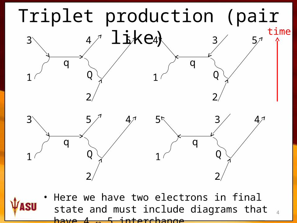
Triplet production (pair like)
• Here we have two electrons in final state and must include diagrams that have 4 ↔ 5 interchange
1
2
3 4 5
qQ 1
2
4 3 5
1
2
3 5 4
qQ 1
2
5 3 4
time

5
Triplet production (Compton like)
• Includes 4 ↔ 5 exchange
1 2
4 Q
q
5 3
1 2
4 Q
5 3
1 2
5 Q
q
4 3
1 2
5 Q
4 3
time

M. Dugger, February 2014 6
Screening correction

7
Screening correction
• Leonard Maximon informed me that the screening correction for triplet production should not be important for the beam asymmetry but was very important for the cross section
• Used the screening correction provided in the paper by Maximon and Gimm [1] to compare cross section results of the event generator to values from the NIST
[1] L. C. Maximon, H. A. Gimm Phys. Rev. A. 23, 1, (1981).
8
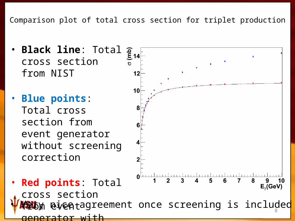
Comparison plot of total cross section for triplet production
• Black line: Total cross section from NIST
• Blue points: Total cross section from event generator without screening correction
• Red points: Total cross section from event generator with screening corrections included
• Very nice agreement once screening is included

9
Most important diagrams
•The Mork paper [2] says that the Compton-like diagrams and the switched electron leg diagrams should be negligible at high photon energy
[2] K. J. Mork Phys. Rev. 160, 5, (1967).
10
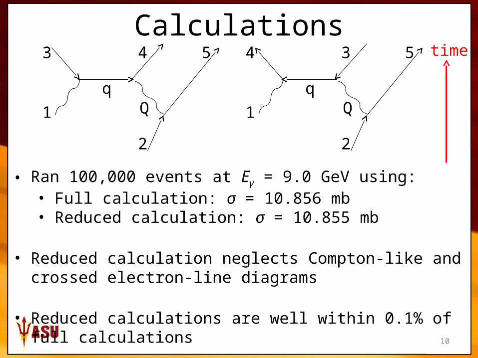
Calculations
• Ran 100,000 events at Eγ = 9.0 GeV using:• Full calculation: σ = 10.856 mb• Reduced calculation: σ = 10.855 mb
• Reduced calculation neglects Compton-like and crossed electron-line diagrams
• Reduced calculations are well within 0.1% of full calculations
1
2
3 4 5
qQ 1
2
4 3 5
time
M. Dugger, February 2012 11
Comparison of GEANT4 study of triplet polarimeter to previous study
• The SAL detector
• δ-rays
• Pair to triplet ratio
• ASU simulation of SAL
• Could SAL have been modified to work in the Hall-D environment?
M. Dugger, February 2012 12
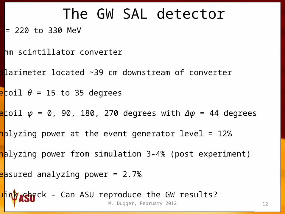
The GW SAL detector• Eγ = 220 to 330 MeV
• 2 mm scintillator converter
• Polarimeter located ~39 cm downstream of converter
• Recoil θ = 15 to 35 degrees
• Recoil φ = 0, 90, 180, 270 degrees with Δφ = 44 degrees
• Analyzing power at the event generator level = 12%
• Analyzing power from simulation 3-4% (post experiment)
• Measured analyzing power = 2.7%
• Quick check - Can ASU reproduce the GW results?
M. Dugger, February 2012 13
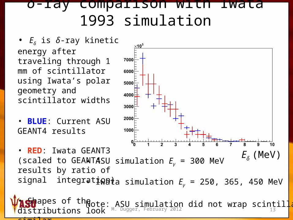
δ-ray comparison with Iwata 1993 simulation
• Eδ is δ-ray kinetic energy after traveling through 1 mm of scintillator using Iwata’s polar geometry and scintillator widths
• BLUE: Current ASU GEANT4 results
• RED: Iwata GEANT3 (scaled to GEANT4 results by ratio of signal integration)
• Shapes of the distributions look similar
Eδ (MeV)• ASU simulation Eγ = 300 MeV • Iwata simulation Eγ = 250, 365, 450 MeV
Note: ASU simulation did not wrap scintillators
M. Dugger, February 2012 14
NIST cross sections for triplet and pair production off carbon
• σpair/σtriplet:5.75 @ 300 MeV5.16 @ 9.0 GeV
• Ratio does not vary much over large energy range
M. Dugger, February 2012 15
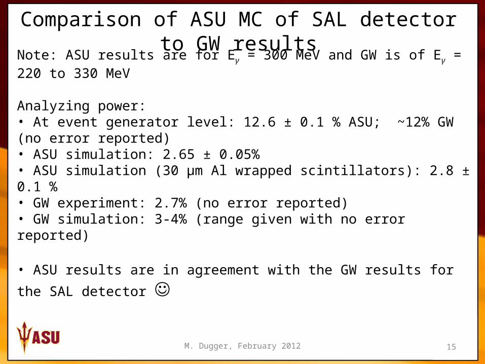
Comparison of ASU MC of SAL detector to GW resultsNote: ASU results are for Eγ = 300 MeV and GW is of Eγ = 220 to 330 MeV
Analyzing power: • At event generator level: 12.6 ± 0.1 % ASU; ~12% GW (no error reported)• ASU simulation: 2.65 ± 0.05%• ASU simulation (30 μm Al wrapped scintillators): 2.8 ± 0.1 % • GW experiment: 2.7% (no error reported)• GW simulation: 3-4% (range given with no error reported)
• ASU results are in agreement with the GW results for the SAL detector ☺
M. Dugger, February 2012 16
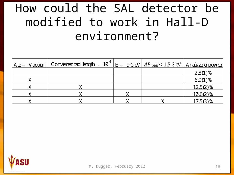
How could the SAL detector be modified to work in Hall-D environment?
Air → Vacuum Converter rad length → 10-4E → 9 GeV ΔE pair < 1.5 GeV Analyzing power
2.8(1) %X 6.9(1) %X X 12.5(2) %X X X 10.6(2) %X X X X 17.5(3) %
M. Dugger, February 2012 17
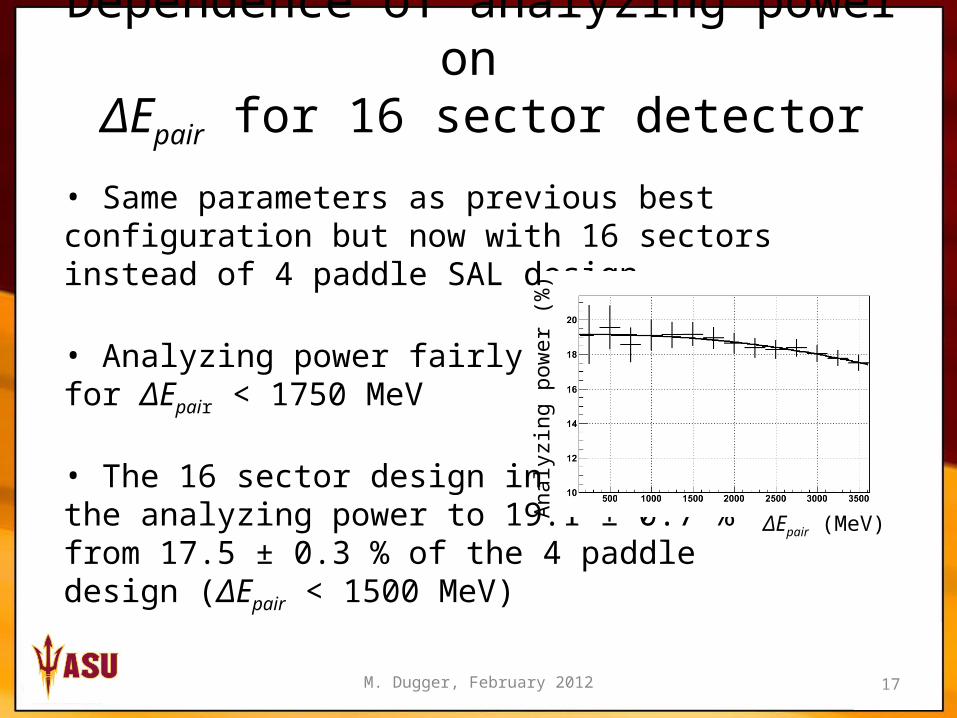
Dependence of analyzing power on ΔEpair for 16 sector detector
• Same parameters as previous best configuration but now with 16 sectors instead of 4 paddle SAL design
• Analyzing power fairly constantfor ΔEpair < 1750 MeV
• The 16 sector design increasesthe analyzing power to 19.1 ± 0.7 %from 17.5 ± 0.3 % of the 4 paddledesign (ΔEpair < 1500 MeV)
ΔEpair (MeV)A
naly
zing
pow
er (
%)
M. Dugger, February 2012 18
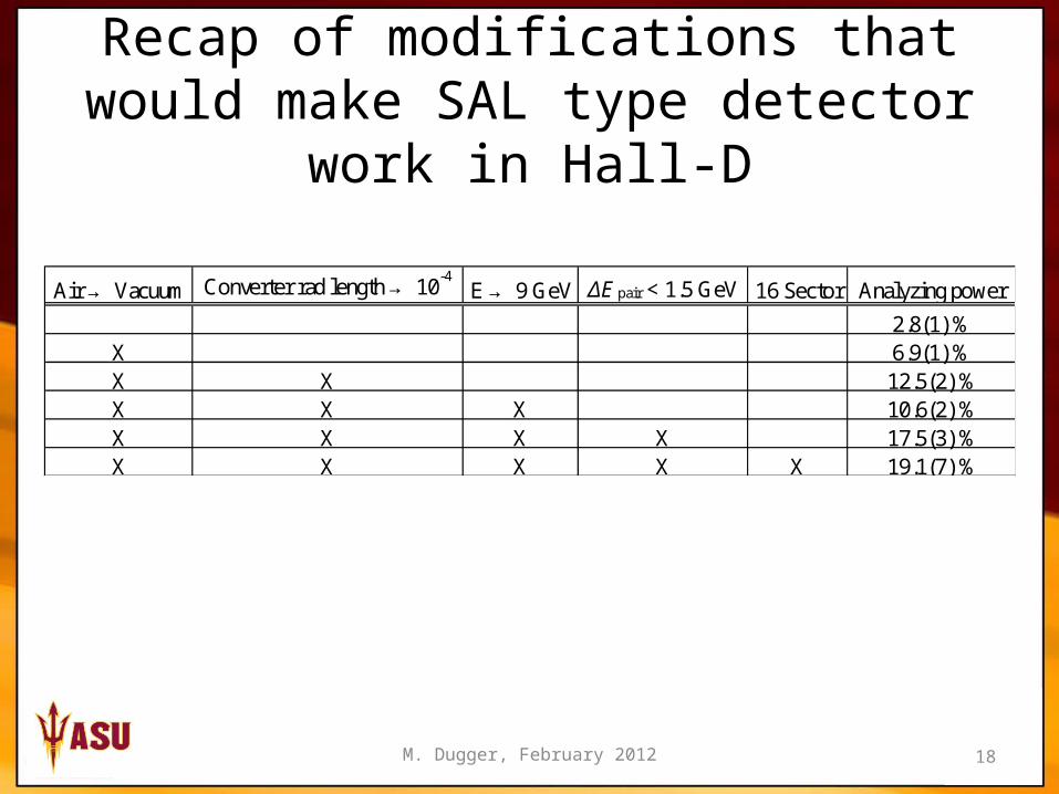
Recap of modifications that would make SAL type detector work in Hall-D
Air → Vacuum Converter rad length → 10-4E → 9 GeV ΔE pair < 1.5 GeV 16 Sector Analyzing power
2.8(1) %X 6.9(1) %X X 12.5(2) %X X X 10.6(2) %X X X X 17.5(3) %X X X X X 19.1(7) %
19
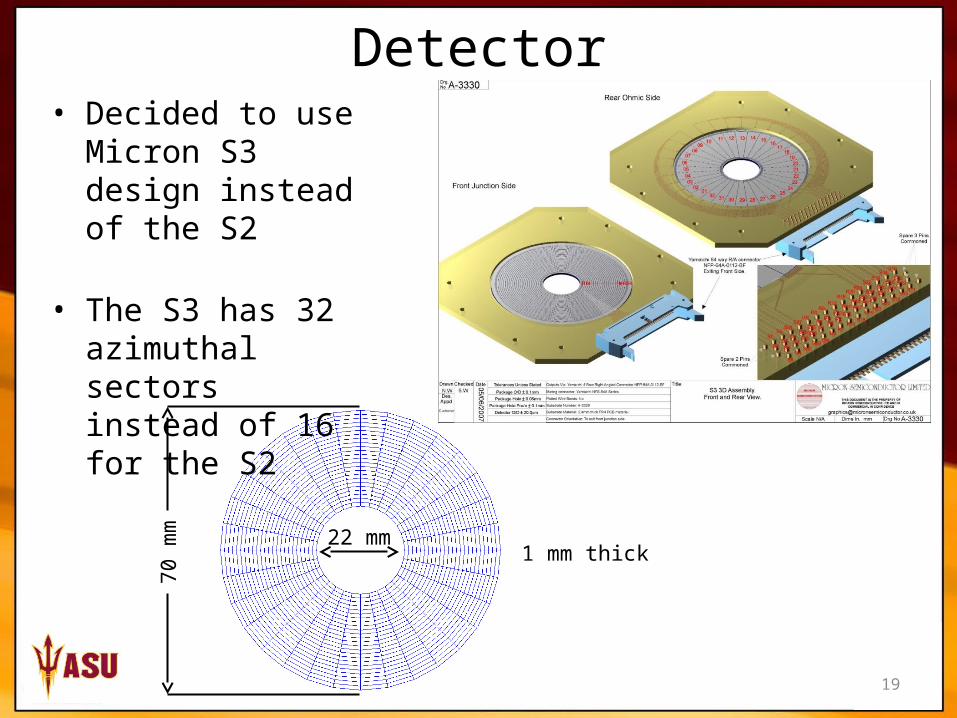
Detector• Decided to use
Micron S3 design instead of the S2
• The S3 has 32 azimuthal sectors instead of 16 for the S2
22 mm
70 m
m
1 mm thick
20
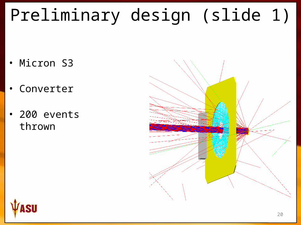
Preliminary design (slide 1)
• Micron S3
• Converter
• 200 events thrown
21
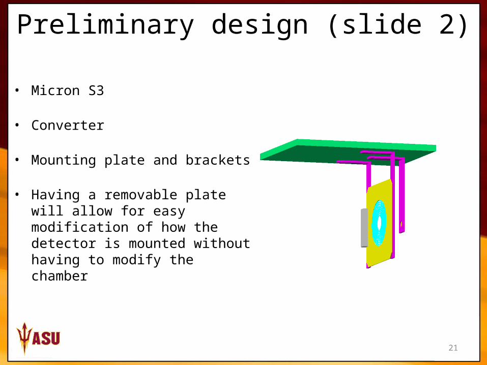
• Micron S3
• Converter
• Mounting plate and brackets
• Having a removable plate will allow for easy modification of how the detector is mounted without having to modify the chamber
Preliminary design (slide 2)
22
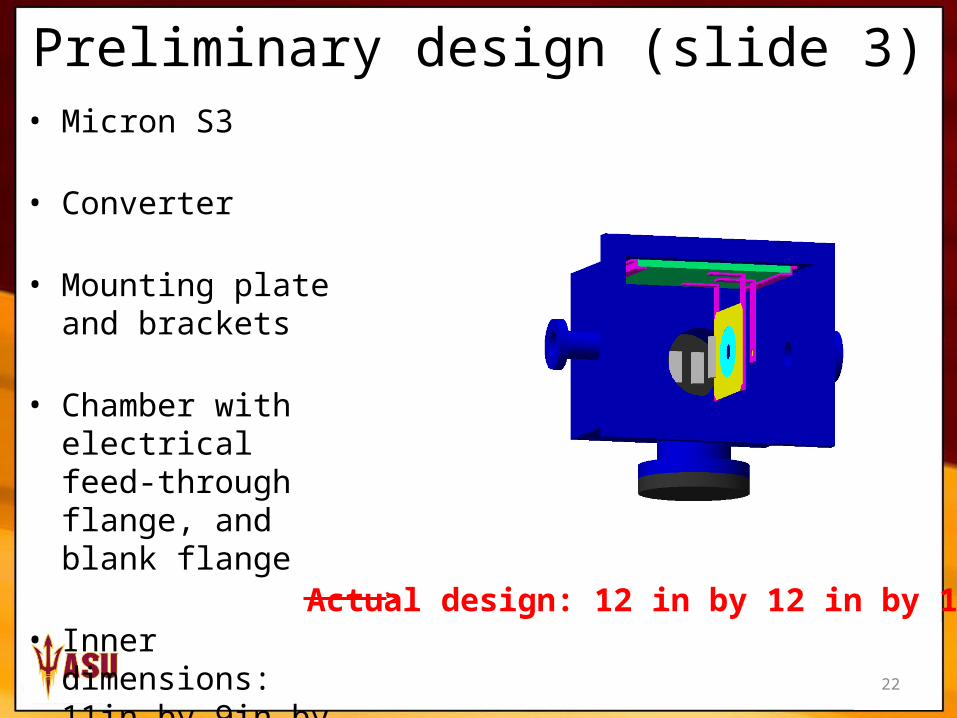
• Micron S3
• Converter
• Mounting plate and brackets
• Chamber with electrical feed-through flange, and blank flange
• Inner dimensions: 11in by 9in by 9in
Preliminary design (slide 3)
Actual design: 12 in by 12 in by 12 in
23
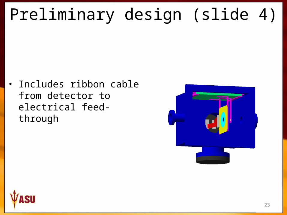
• Includes ribbon cable from detector to electrical feed-through
Preliminary design (slide 4)
24
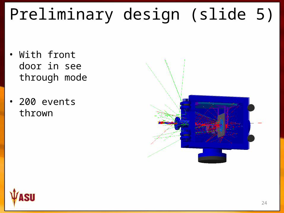
• With front door in see through mode
• 200 events thrown
Preliminary design (slide 5)
25
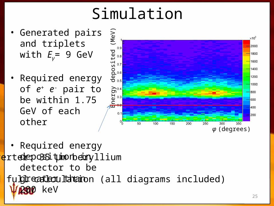
Simulation
φ (degrees)
Ene
rgy
depo
site
d (M
eV)
• Generated pairs and triplets with Eγ= 9 GeV
• Required energy of e+ e- pair to be within 1.75 GeV of each other
• Required energy deposition in detector to be greater than 200 keV
• Converter: 35 μm beryllium • Used full calculation (all diagrams included)
26
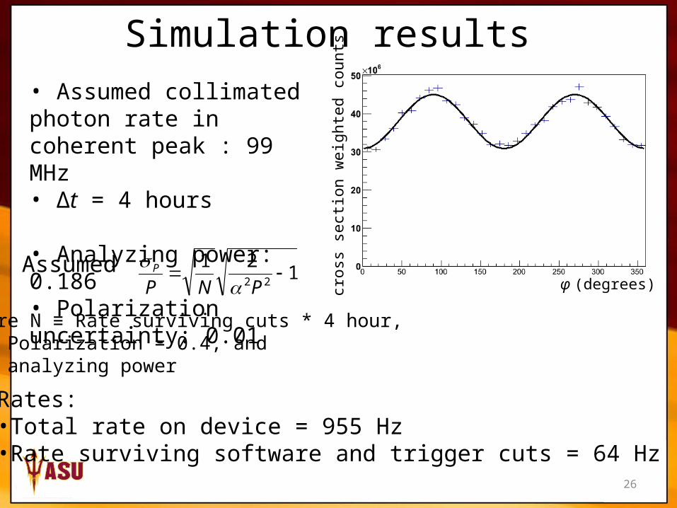
Simulation results
cros
s se
ctio
n w
eigh
ted
coun
ts
φ (degrees)
• Assumed collimated photon rate in coherent peak : 99 MHz• Δt = 4 hours
• Analyzing power: 0.186• Polarization uncertainty: 0.01
Rates: •Total rate on device = 955 Hz•Rate surviving software and trigger cuts = 64 Hz
121
22
PNPP
where N ≡ Rate surviving cuts * 4 hour,P ≡ Polarization = 0.4, andα ≡ analyzing power
Assumed
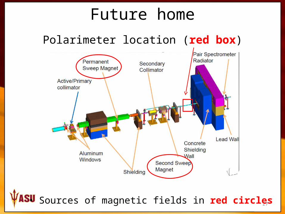
Polarimeter location (red box)
27
Future home
• Sources of magnetic fields in red circles
28
B-field study
• Study performed in April 2012
• Applied magnetic field in vertical direction
M. Dugger, April 2012 29
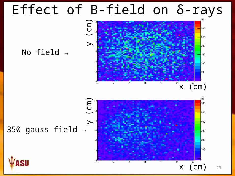
Effect of B-field on δ-rays
x (cm)
x (cm)
y (c
m)
y (c
m)
No field →
350 gauss field →
30
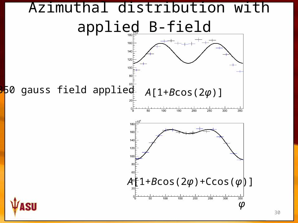
Azimuthal distribution with applied B-field
φ
• 350 gauss field applied A[1+Bcos(2φ)]
A[1+Bcos(2φ)+Ccos(φ)]
31
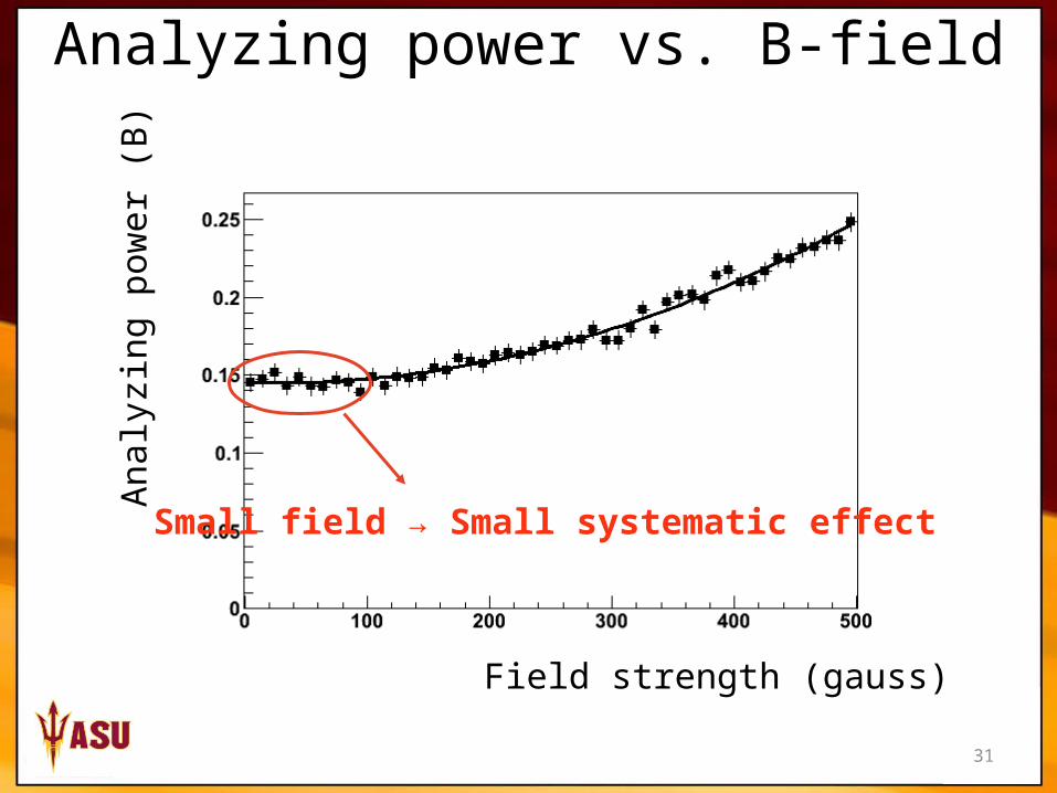
Analyzing power vs. B-field
Ana
lyzi
ng p
ower
(B
)
Field strength (gauss)
Small field → Small systematic effect
32
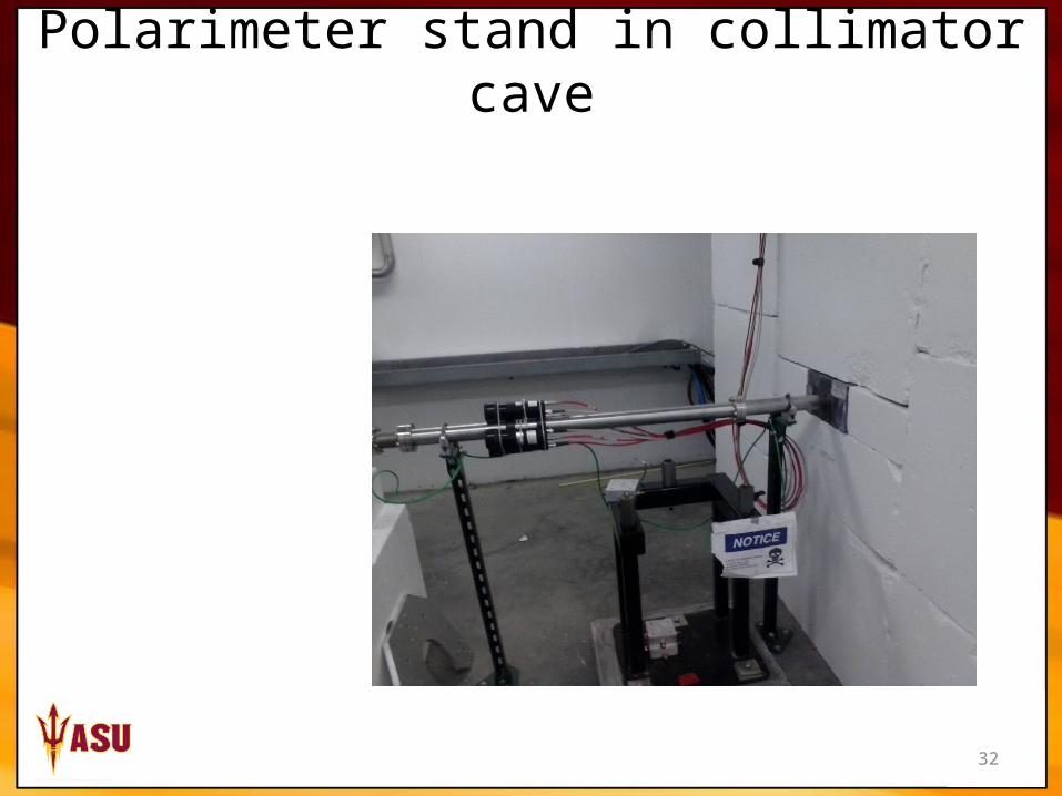
Polarimeter stand in collimator cave
33
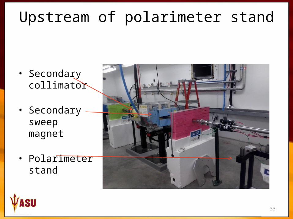
Upstream of polarimeter stand
• Secondary collimator
• Secondary sweep magnet
• Polarimeter stand
34
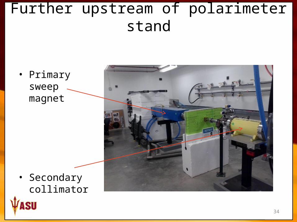
Further upstream of polarimeter stand
• Primary sweep magnet
• Secondary collimator

35
Construction
36
Vacuum system
• When the polarimeter is installed in the collimator cave, the vacuum will come from the beam line
• In the test bench, the vacuum has to be provided by a temporary system
• Using a rotary vane pump for the vacuum system of the test bench
• Rotary vane pumps will back-stream oil and this issue must be addressed
37
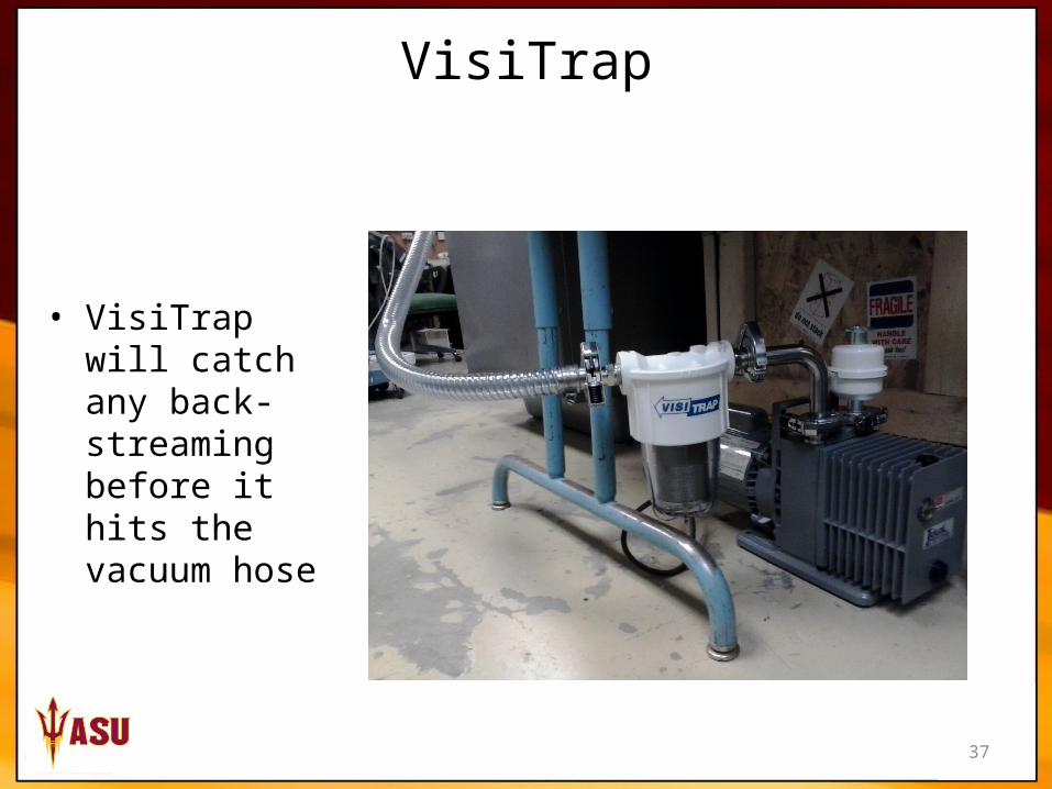
VisiTrap
• VisiTrap will catch any back-streaming before it hits the vacuum hose
38
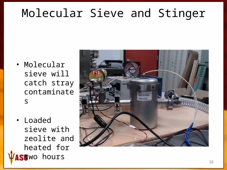
Molecular Sieve and Stinger
• Molecular sieve will catch stray contaminates
• Loaded sieve with zeolite and heated for two hours
39
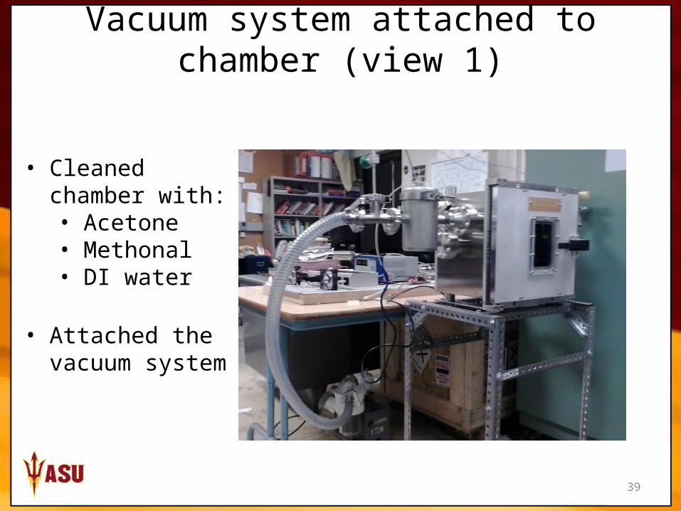
Vacuum system attached to chamber (view 1)
• Cleaned chamber with:• Acetone• Methonal• DI water
• Attached the vacuum system
40
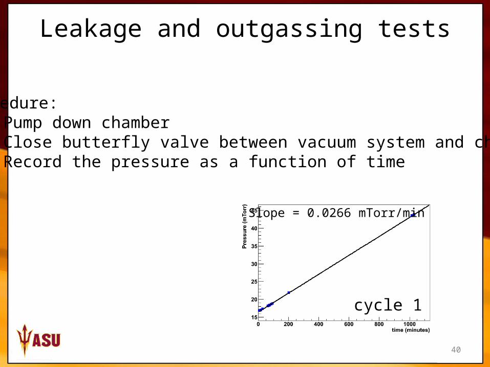
Leakage and outgassing tests
Procedure:• Pump down chamber• Close butterfly valve between vacuum system and chamber• Record the pressure as a function of time
cycle 1
Slope = 0.0266 mTorr/min
41
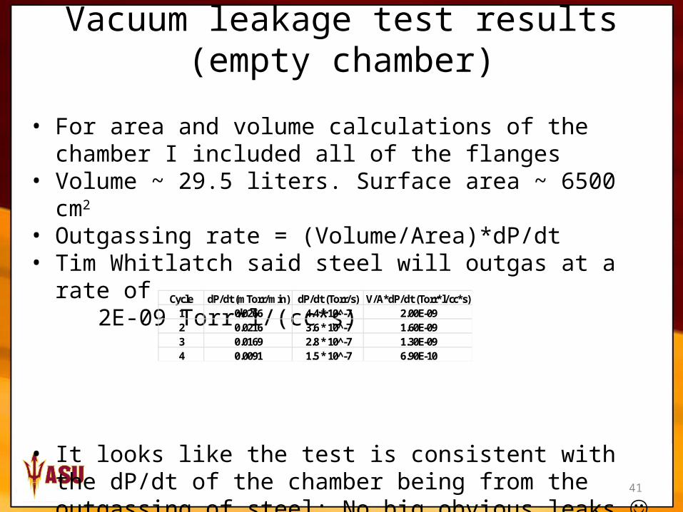
Vacuum leakage test results (empty chamber)
• For area and volume calculations of the chamber I included all of the flanges
• Volume ~ 29.5 liters. Surface area ~ 6500 cm2 • Outgassing rate = (Volume/Area)*dP/dt• Tim Whitlatch said steel will outgas at a rate of 2E-09 Torr*l/(cc*s)
• It looks like the test is consistent with the dP/dt of the chamber being from the outgassing of steel: No big obvious leaks
Cycle dP/dt (mTorr/min) dP/dt (Torr/s) V/A*dP/dt (Torr*l/cc*s)1 0.0266 4.4 * 10^-7 2.00E-092 0.0216 3.6 * 10^-7 1.60E-093 0.0169 2.8 * 10^-7 1.30E-094 0.0091 1.5 * 10^-7 6.90E-10
42
• Five hour pump down to ~20 mTorr
• Ql = V*dp/dt found to be 1.80x10⁻⁴ Torr*liter/s
• A turbo pump on the chamber with a flow rate of 100 liters/s with a working pressure of 2x10⁻⁵ Torr will have a Qw = 2x10⁻³ Torr*liter/s
• Pfeiffer vacuum says that a system is adequately tight if Qw > 10*Ql
• Putting a turbo pump with flow rate 100 liters/s on the base of the chamber should be sufficient to maintain a vacuum of 2x10⁻⁵ Torr
Vacuum test results (detector in chamber)
43
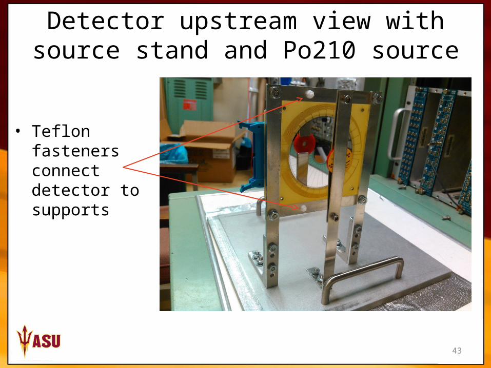
Detector upstream view with source stand and Po210 source
• Teflon fasteners connect detector to supports
44
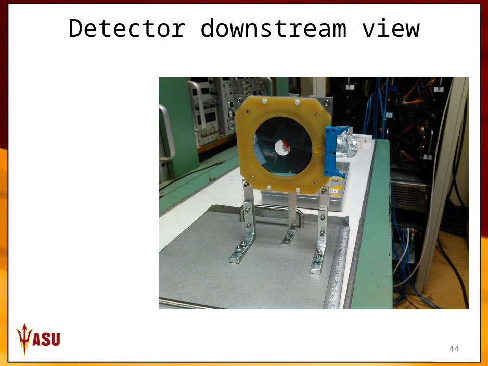
Detector downstream view
45
Preamps
• Decided to have a parallel development of the preamps:• Glasgow is building a pre-amplification system based off
of the Rutherford Appleton Laboratory RAL-108 pramps and custom motherboards
• ASU is using a pre-amplification system from Swan research (“Box16 preamps”)
46
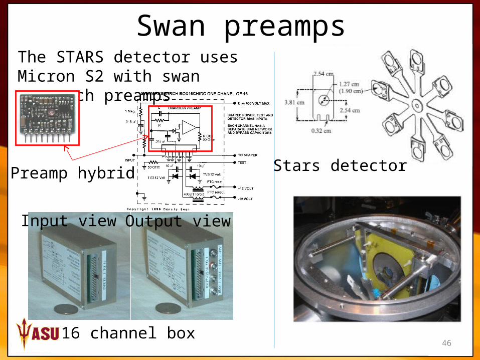
Swan preampsThe STARS detector uses Micron S2 with swan research preamps
Input view Output view
16 channel box
Preamp hybrid Stars detector
47
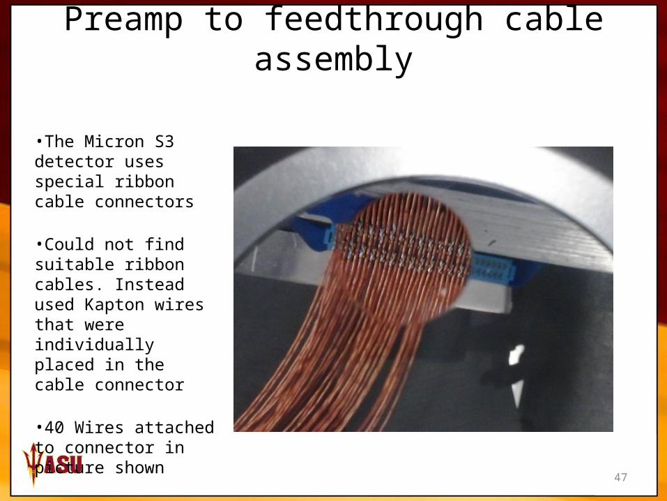
Preamp to feedthrough cable assembly
•The Micron S3 detector uses special ribbon cable connectors
•Could not find suitable ribbon cables. Instead used Kapton wires that were individually placed in the cable connector
•40 Wires attached to connector in picture shown
48
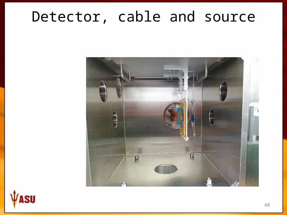
Detector, cable and source
49
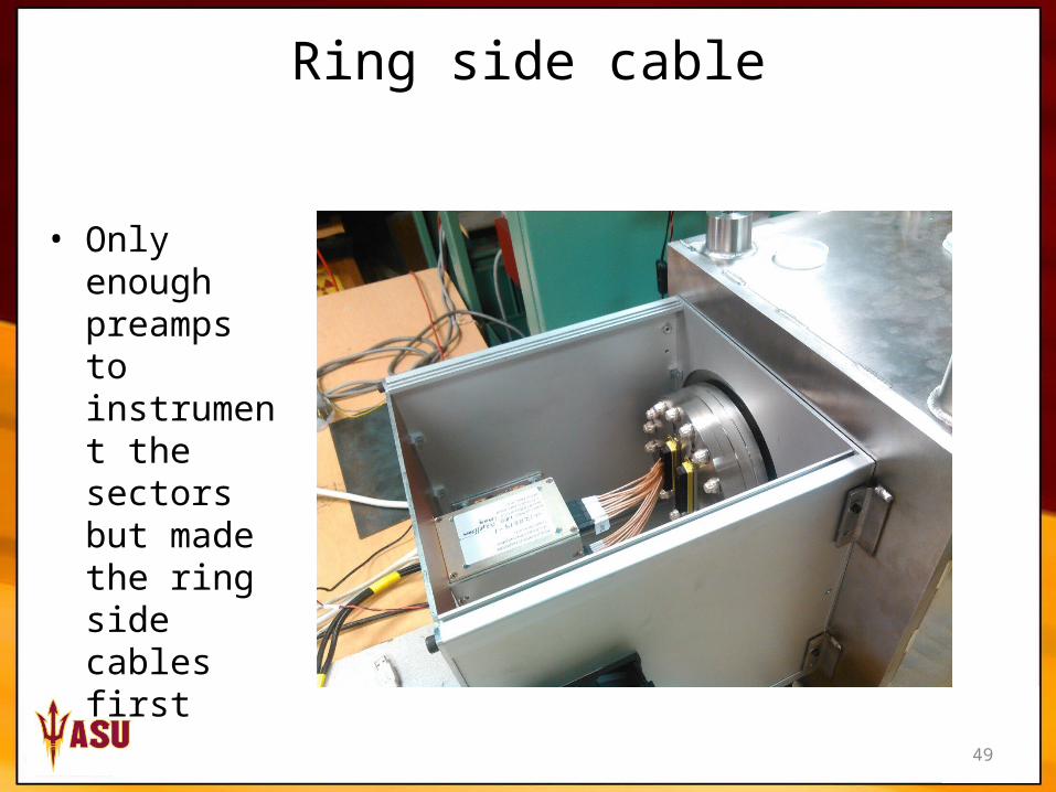
Ring side cable
• Only enough preamps to instrument the sectors but made the ring side cables first
50
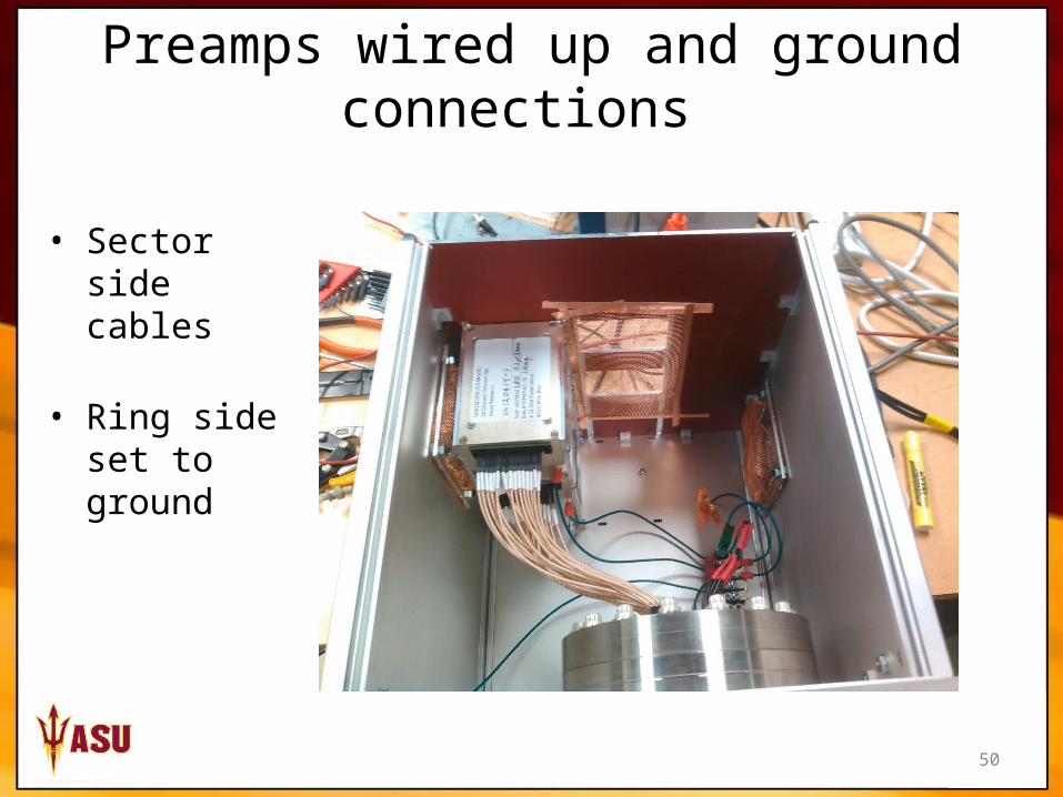
Preamps wired up and ground connections
• Sector side cables
• Ring side set to ground
51
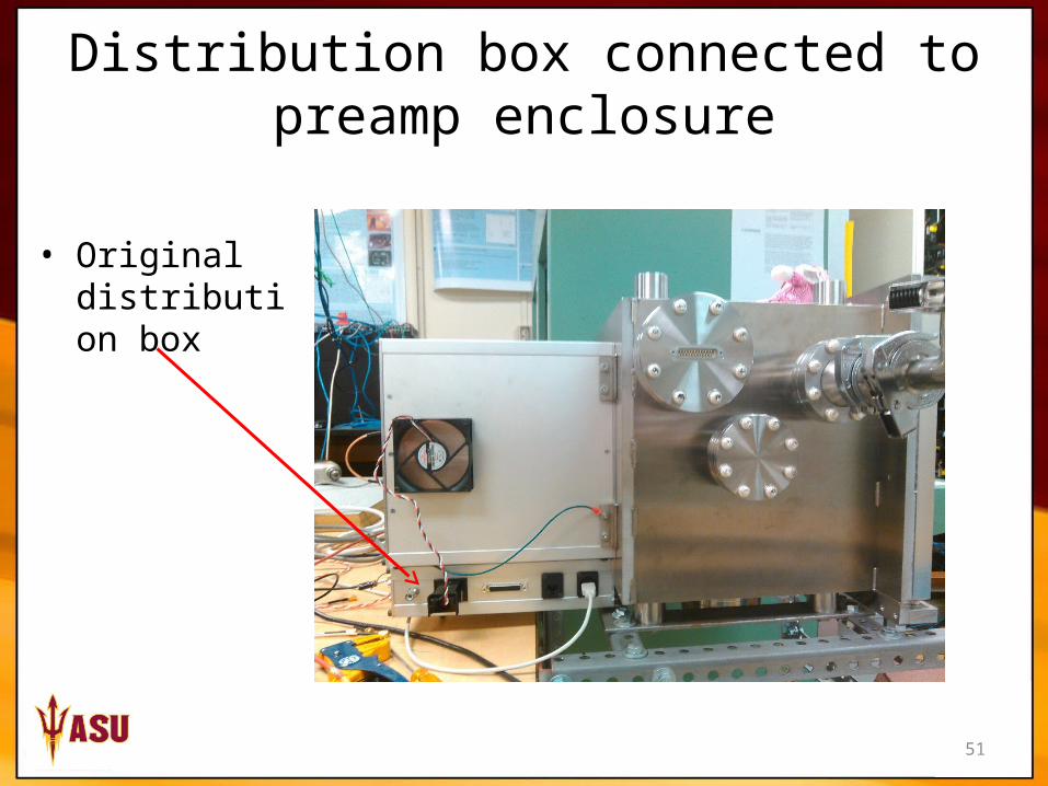
Distribution box connected to preamp enclosure
• Original distribution box
52
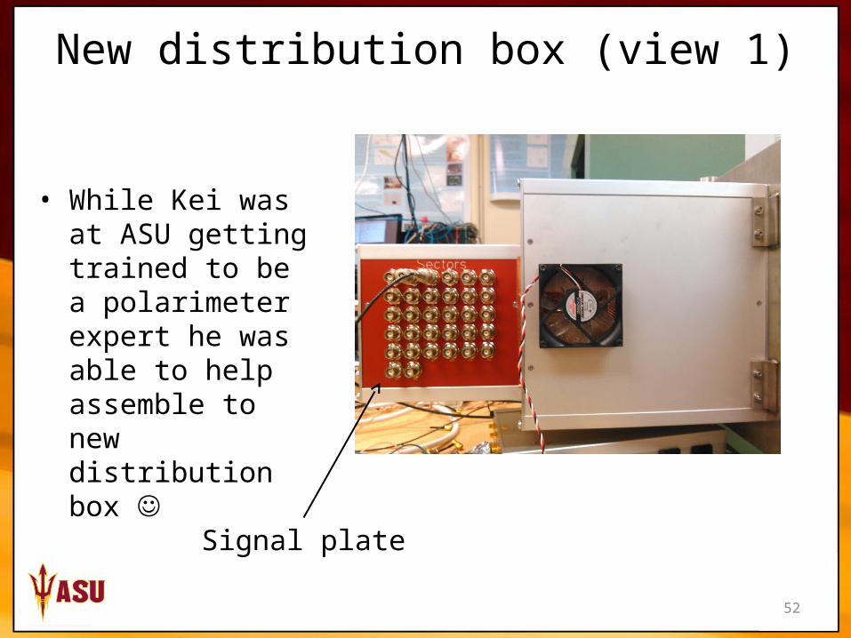
New distribution box (view 1)
• While Kei was at ASU getting trained to be a polarimeter expert he was able to help assemble to new distribution box
Signal plate
53
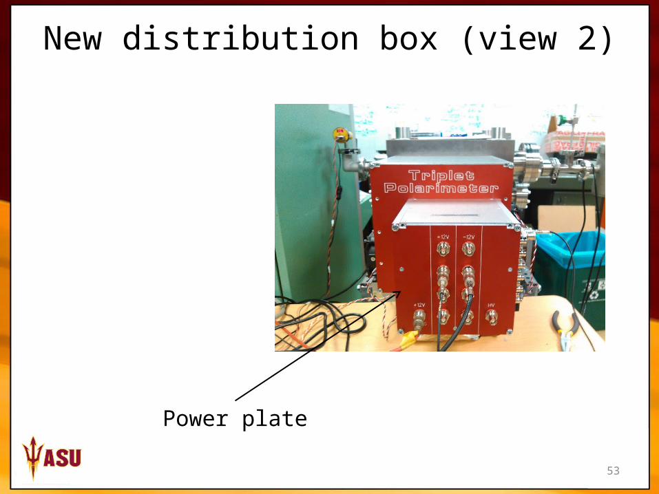
New distribution box (view 2)
Power plate
54
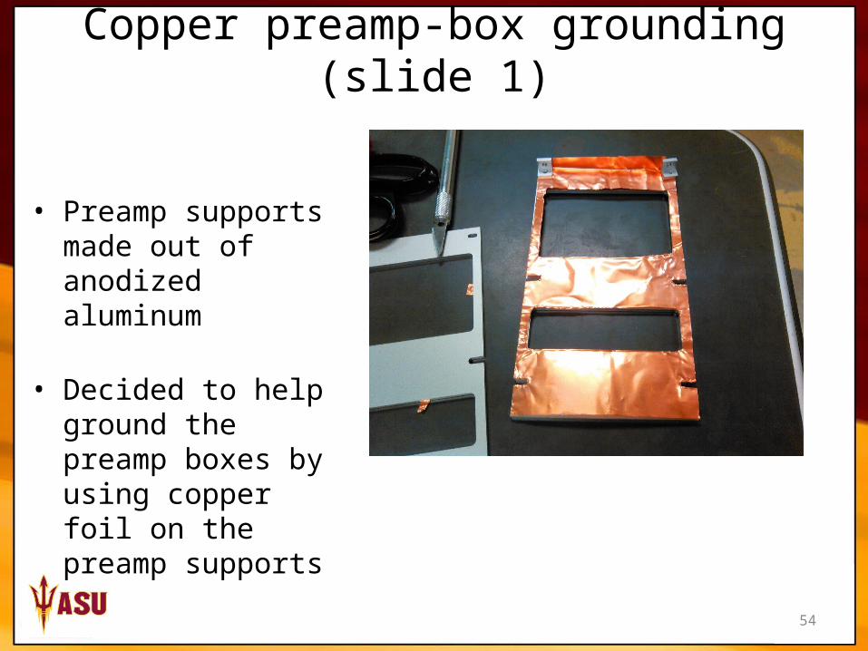
Copper preamp-box grounding (slide 1)
• Preamp supports made out of anodized aluminum
• Decided to help ground the preamp boxes by using copper foil on the preamp supports
55
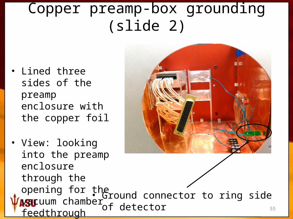
Copper preamp-box grounding (slide 2)
• Lined three sides of the preamp enclosure with the copper foil
• View: looking into the preamp enclosure through the opening for the vacuum chamber feedthrough flange
• Ground connector to ring side of detector
56
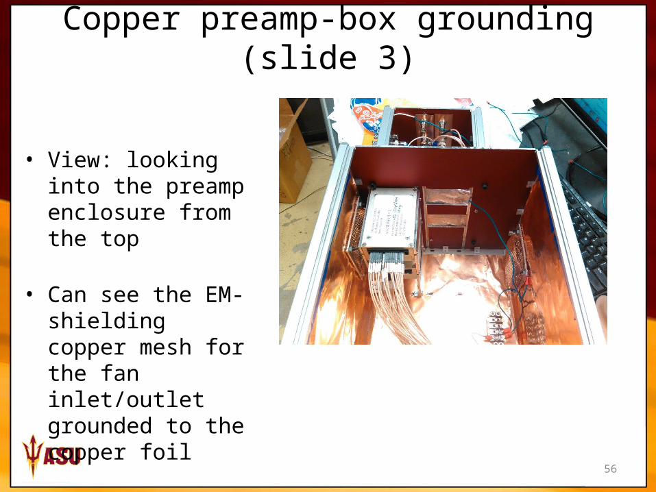
Copper preamp-box grounding (slide 3)
• View: looking into the preamp enclosure from the top
• Can see the EM-shielding copper mesh for the fan inlet/outlet grounded to the copper foil
57
Signal plate grounding
• Cutting copper foil for the signal plate grounding
• Also grounded to the input voltages (power plate)
58
Signal plate and power plate grounding
59
Fan leads
• Routed the fan leads through the preamp enclosure towards the distribution box
60
View of polarimeter with original distribution box completely removed
61
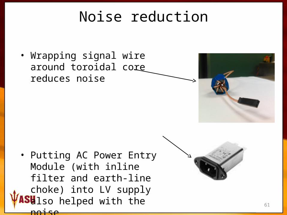
• Wrapping signal wire around toroidal core reduces noise
• Putting AC Power Entry Module (with inline filter and earth-line choke) into LV supply also helped with the noise
Noise reduction
62
The silicon detector
• The detector is very much like a diode operated in reverse bias mode
• As the voltage is increased across the detector, the depletion region gets larger
• The larger the depletion region, the smaller the capacitance of the detector
• For each 3.6 eV of energy deposited in the depletion region there is one electron-hole pair that is created and then swept out of the detector
63
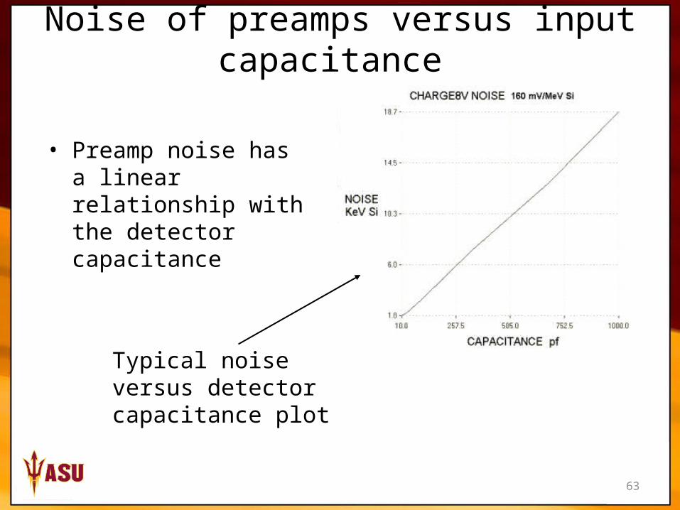
Noise of preamps versus input capacitance
• Preamp noise has a linear relationship with the detector capacitance
Typical noise versus detector capacitance plot
64
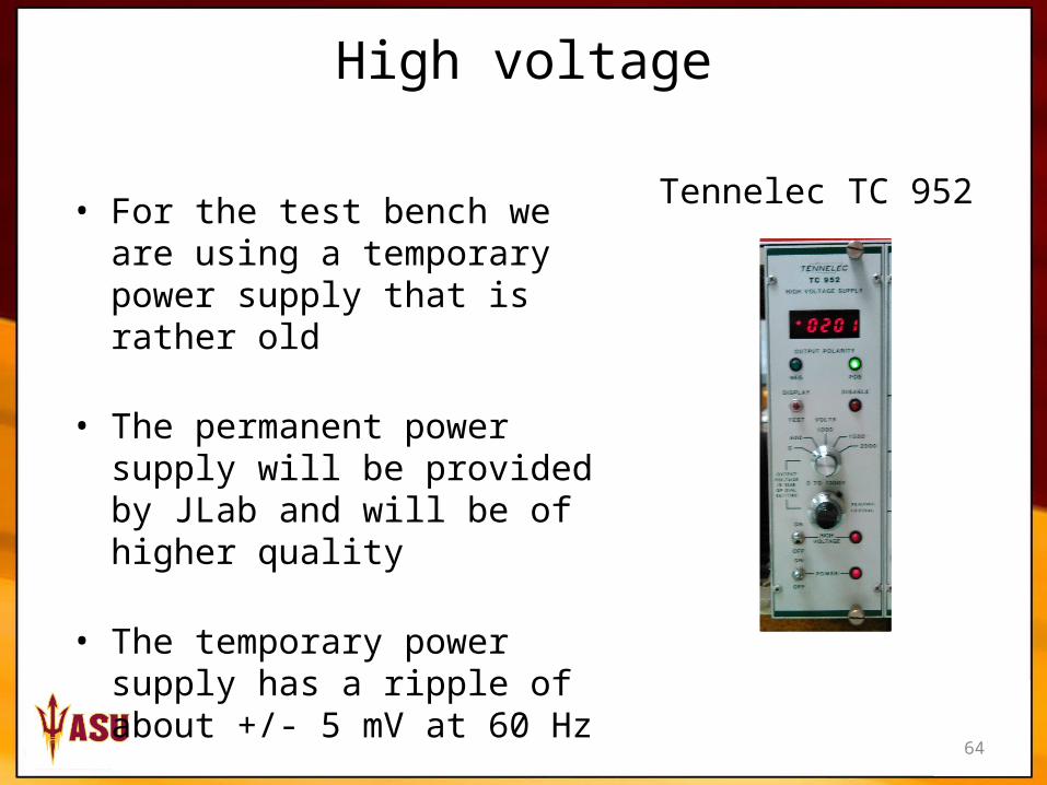
High voltage
Tennelec TC 952• For the test bench we are using a temporary power supply that is rather old
• The permanent power supply will be provided by JLab and will be of higher quality
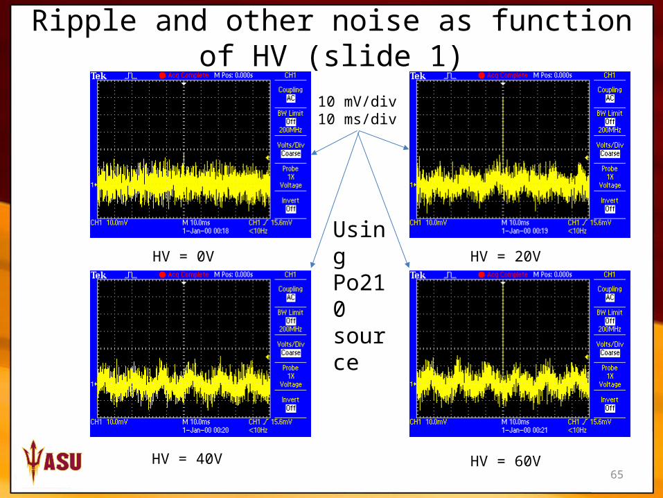
• The temporary power supply has a ripple of about +/- 5 mV at 60 Hz
65
Ripple and other noise as function of HV (slide 1)
HV = 0V HV = 20V
HV = 40V HV = 60V
10 mV/div10 ms/div
Using Po210 source
66
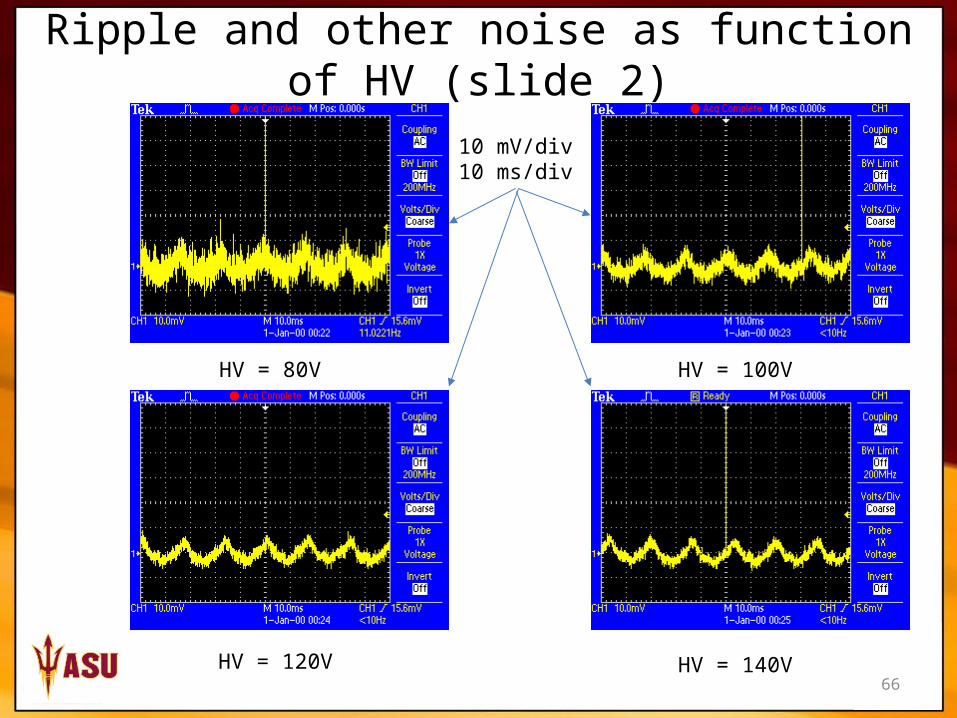
Ripple and other noise as function of HV (slide 2)
HV = 80V HV = 100V
HV = 120V HV = 140V
10 mV/div10 ms/div
67
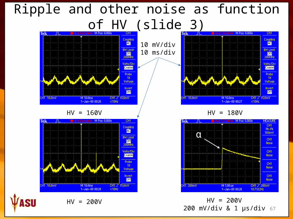
Ripple and other noise as function of HV (slide 3)
HV = 160V HV = 180V
HV = 200V HV = 200V200 mV/div & 1 µs/div
10 mV/div10 ms/div
α
68
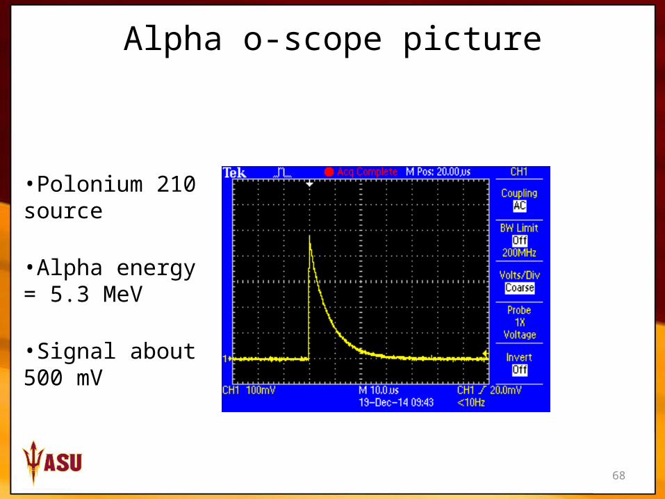
Alpha o-scope picture
•Polonium 210 source
•Alpha energy = 5.3 MeV
•Signal about 500 mV
69
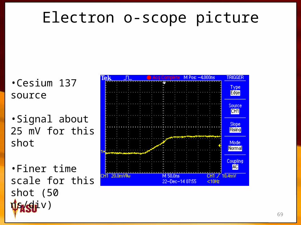
Electron o-scope picture
•Cesium 137 source
•Signal about 25 mV for this shot
•Finer time scale for this shot (50 ns/div)
70
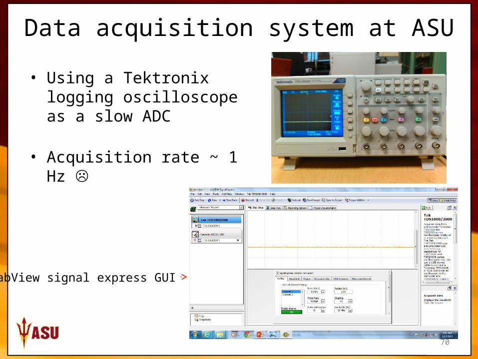
Data acquisition system at ASU
• Using a Tektronix logging oscilloscope as a slow ADC
• Acquisition rate ~ 1 Hz
LabView signal express GUI
71
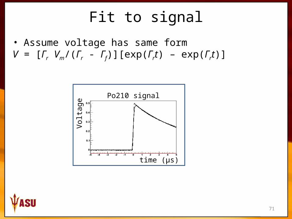
Fit to signal
• Assume voltage has same formV = [Γr Vm/(Γr - Γf)][exp(Γrt) – exp(Γrt)]
Vol
tage
time (μs)
Po210 signal
72
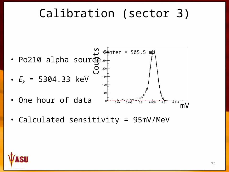
Calibration (sector 3)
Cou
nts
mV
Center = 505.5 mV
• Po210 alpha source
• Ek = 5304.33 keV
• One hour of data
• Calculated sensitivity = 95mV/MeV
73
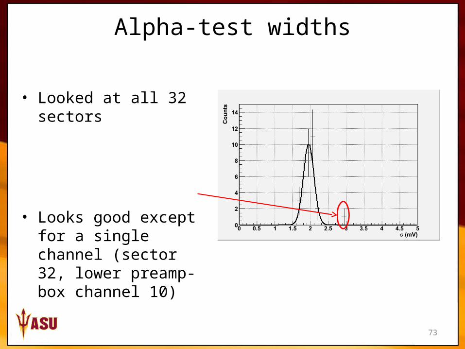
Alpha-test widths
• Looked at all 32 sectors
• Looks good except for a single channel (sector 32, lower preamp-box channel 10)
74
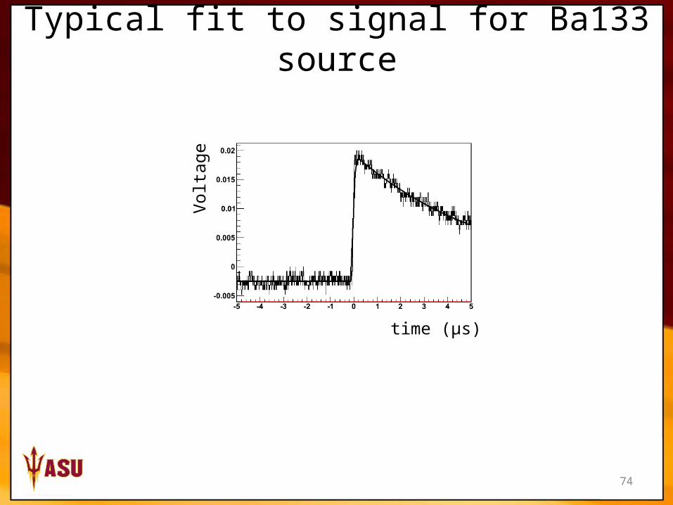
Typical fit to signal for Ba133 source
Vol
tage
time (μs)
75
MC Data
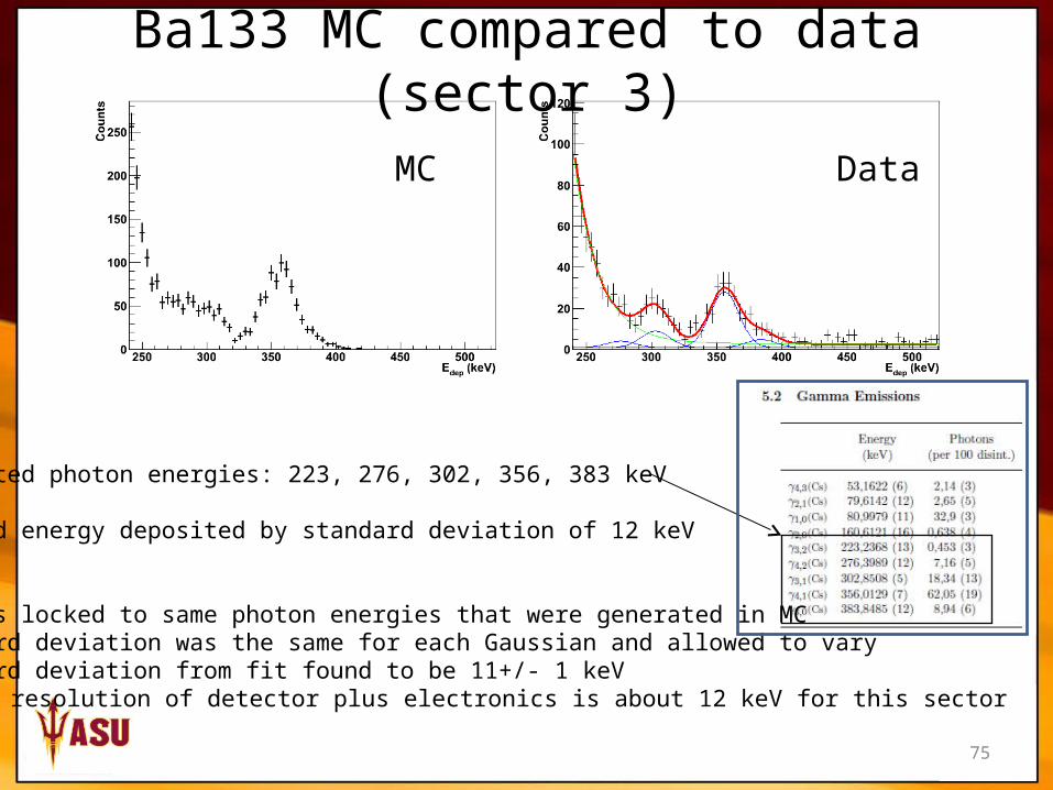
• MC• Generated photon energies: 223, 276, 302, 356, 383 keV
• Smeared energy deposited by standard deviation of 12 keV
• Fit:• Centers locked to same photon energies that were generated in MC• Standard deviation was the same for each Gaussian and allowed to vary• Standard deviation from fit found to be 11+/- 1 keV
• Therefore, resolution of detector plus electronics is about 12 keV for this sector
Ba133 MC compared to data (sector 3)
76
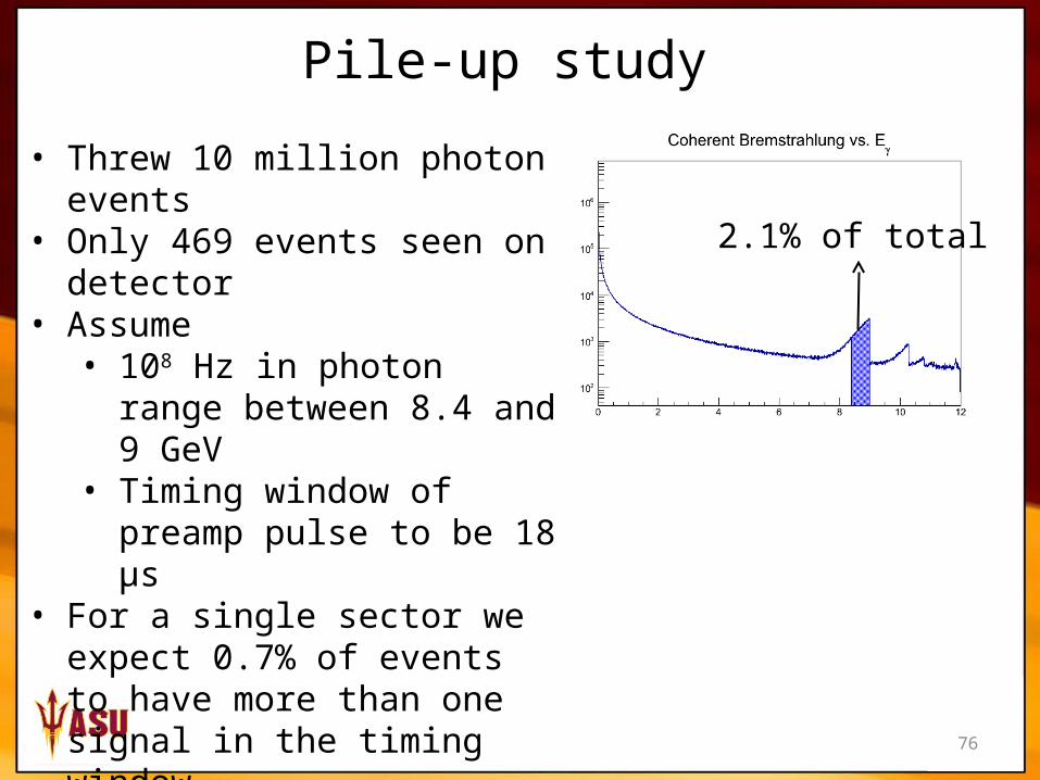
Pile-up study
2.1% of total
• Threw 10 million photon events• Only 469 events seen on detector• Assume• 108 Hz in photon range
between 8.4 and 9 GeV• Timing window of preamp
pulse to be 18 μs • For a single sector we expect 0.7%
of events to have more than one signal in the timing window
• Pile-up should not be much of an issue

77
Work still to be done at ASU
• Need to complete the positioning system (should be able to finish this week)
78
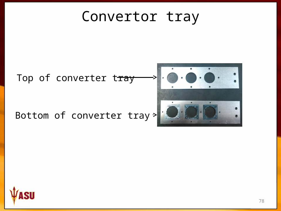
Convertor tray
Bottom of converter tray
Top of converter tray
79
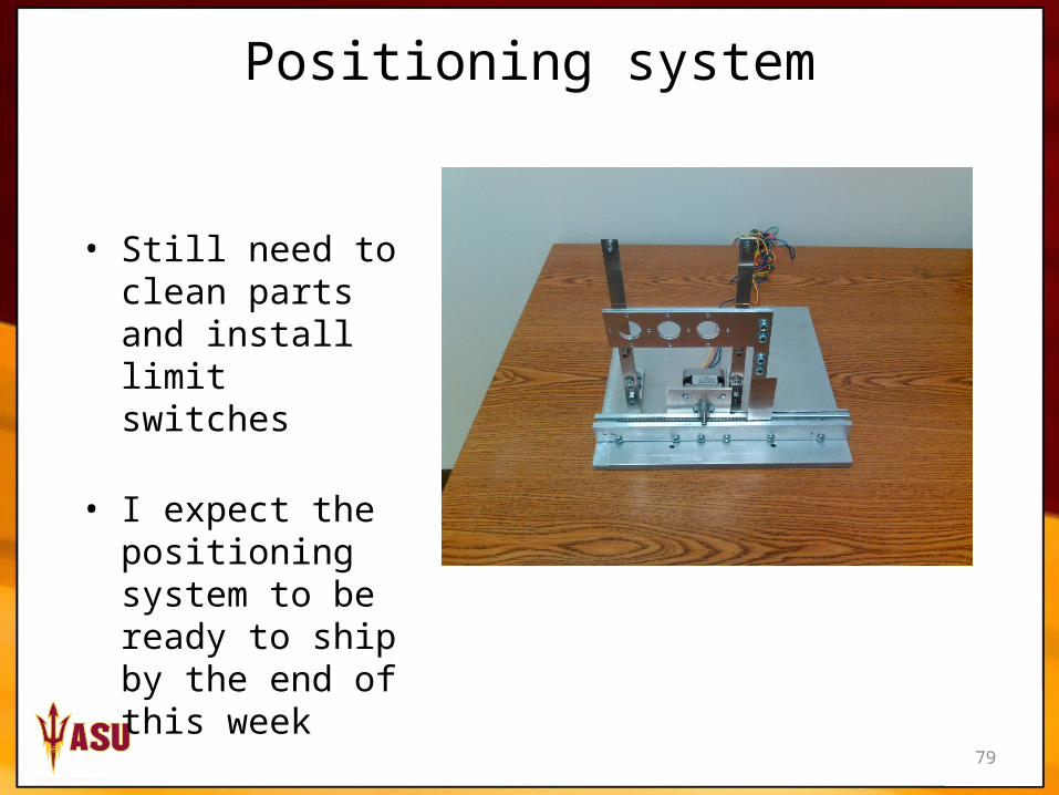
Positioning system
• Still need to clean parts and install limit switches
• I expect the positioning system to be ready to ship by the end of this week
80
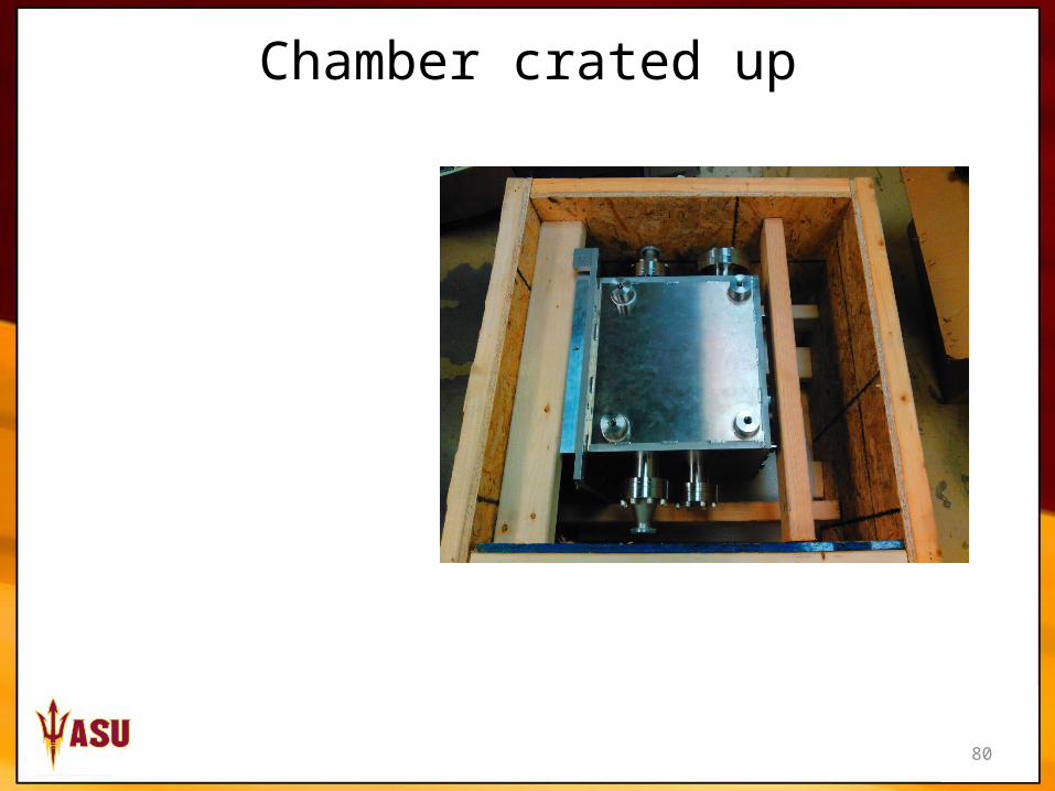
Chamber crated up
81
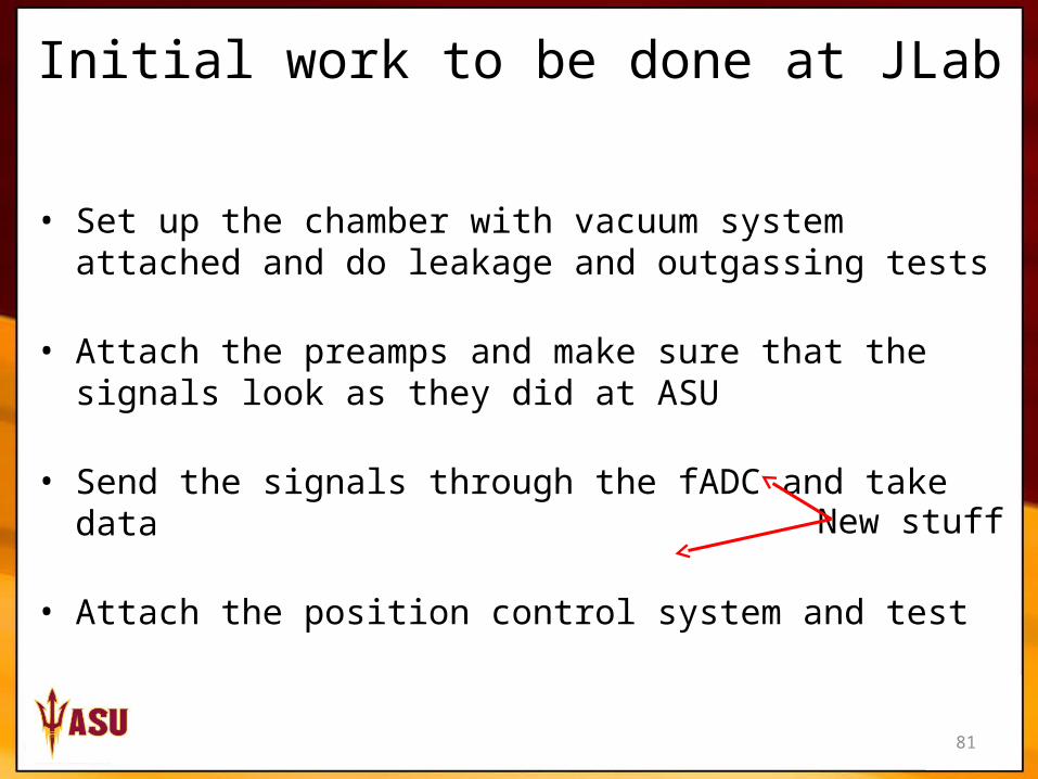
Initial work to be done at JLab
• Set up the chamber with vacuum system attached and do leakage and outgassing tests
• Attach the preamps and make sure that the signals look as they did at ASU
• Send the signals through the fADC and take data
• Attach the position control system and testNew stuff
82
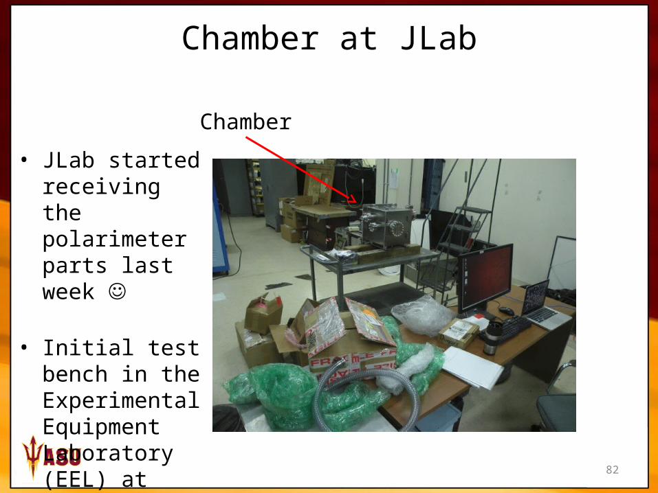
Chamber
Chamber at JLab
• JLab started receiving the polarimeter parts last week
• Initial test bench in the Experimental Equipment Laboratory (EEL) at Jefferson Lab