1

Paper 128-2012

Constructing a Credit Risk Scorecard using Predictive Clusters

Alejandro Correa, Banco Colpatria, Bogotá, Colombia

Andrés González, Banco Colpatria, Bogotá, Colombia

Catherine Nieto, Banco Colpatria, Bogotá, Colombia

Darwin Amezquita, Banco Colpatria, Bogotá, Colombia

ABSTRACT

Traditionally the cluster analysis has been used as a descriptive tool, in which the algorithm is used to create groups of observations based on their characteristics. In this paper the use of cluster analysis as a part of a predictive algorithm is proposed. This methodology is applied by first determining to which cluster a prospect client belongs, and then calculate a specific credit risk scorecard for each cluster. Results will show that this approach provides better results than using a single scorecard for all the prospect clients.

INTRODUCTION

Globalization has opened markets and intensified competition, making innovation to play a key role in competitiveness. For this reason every idea should be world-wide class, focusing on increasing efficiency, productivity, quality and being cost efficient. This study aims to propose how to innovate by creating new solutions using already well known techniques such as cluster analysis.

The main objective of this paper is to improve the development of credit risk scorecards by using cluster analysis, not only as a methodology to classify individuals with some specific characteristics (variables), but also as a part of a prediction process; obtaining efficient results when it comes to classifying and getting to know the profiles of the new clients that join the financial business. To do this, a comparison of two different methodologies is performed in four different databases in order to obtain an unbiased conclusion. The first methodology consists on developing scorecard models for the entire population using a logistic regression and a Multi-Layer Perceptron neural network (MLP). The second methodology involves four steps; first to carry out a cluster analysis for the entire population using K-means and Kohonen self-organizing map algorithms. Then, to develop an algorithm to assign a new client to any of the resulting clusters; the techniques used for this purpose are the multinomial logistic regression, MLP neural network, minimum Euclidian distance, minimum adjusted distance and Mahalanobis distance. The third step is to develop a scorecard for each of the clusters using also a logistic regression and a MLP neural network. Lastly, a final score is computed using three different techniques: cluster score, score ensemble and classifier average vote ensemble.

To conclude, a contrast between these methodologies is conducted using the F1 score statistic as a measure of comparison.

This paper is divided into five sections. First, some descriptive statistics of the databases used in the analysis are presented. Then, an introduction to the most general concepts of the methodologies used along the paper is made. Subsequently, there is an explanation of the modeling process and the particularities of the algorithms and measures of comparison applied in this paper. In the fourth section the experimental results are shown and finally the conclusions are presented.

DATA

In order to perform a complete analysis of the methodology exposed in this paper and to obtain unbiased significant results, four different databases from different products of a financial institution were used to develop credit risk socrecards. With the default definition found for each specific population, the clients were classified into good or bad. Also since the client’s credit information is confidential, variables were renamed to X1,X2, …, Xn.

Table 1 presents the number of good and bad clients after applying the default definition, the bad rate and the number of variables used for each of the four databases. Also, the original data is randomly divided into three different datasets used for the scorecard development, validation and stability test.

Data Mining and Text AnalyticsSAS Global Forum 2012

2

Data Good Bad Total Bad Rate Number of Variables

Database 1 81.659 5.394 87.053 6,20% 7

Database 2 12.065 2.258 14.323 15,76% 29

Database 3 50.670 3.797 54.467 6,97% 25

Database 4 71.127 54.430 125.557 43,35% 7

Table 1. Databases descriptive information

BACKGROUND

In this section the most general concepts of the methodologies used in this paper such as cluster analysis, logistic regression, neural networks and the measures of distance and comparison between models are presented.

CLUSTER ANALYSIS

Cluster analysis is a descriptive process where the observations of a database are divided into groups called clusters, based on their characteristics. The idea is to create groups between observations that are more similar to each other than to those in other groups. In other words, a cluster is a group of relatively homogeneous clients where the clients of one cluster are dissimilar to clients of another cluster.

In cluster analysis the groups can be created using different types of algorithms. These algorithms define the measures of similarity and therefore how clusters are formed. Some of the most popular algorithms used for clustering are K-means and Kohonen self-organizing map (SOM), which we explain below.

It is important to note that there is not a perfect algorithm, so it depends on the individual characteristics of the data. Additionally, since cluster analysis is an iterative process it involves trail and failure until the desire number of clusters and results are achieved.

o K-Means

K- means clustering is a method that attempts to assign a set of n observations into a k number of

clusters where each observation is allocated to the cluster with the nearest centroid. Therefore each observation can only belong to one cluster. The centroid of a cluster is the mean value for all the observations in the cluster.

There are many heuristic algorithms that are used to reach an optimum assignation of the observations to the clusters; one of the most commonly used algorithms is the Lloyd´s algorithm, commonly known as the standard algorithm or k-means algorithm. This method uses an iterative technique to reach the optimum clustering (MacKay, 2003).

The whole process can be divided in two steps. The first is the assignment step, where each observation is assigned to the cluster with the closest centroid. In the second step the new centroids of the clusters are calculated based on the observations that formed the cluster at the end of step one. This process is repeated until the clusters remain unchanged. The target of this process is to find the best fit to the data, minimizing the within-cluster sum of squares.

For the first assignation of the observations to the clusters, usually a random partition method is used. There most commonly used procedures are: i) to randomly assign a cluster to each observation and then proceed with step two or ii) to randomly select k observation and fix the position of those observations as the centroids of the k clusters.

Now that have been explained how the K-means algorithm works, below the steps are presented in a formal way:

1. Each observation is assigned only to one cluster, with the minimum distance as follow,

where is the standardized mean of the observations that belong to the cluster in the last

iteration. Equation (1) exhibits this procedure.

(1)

2. The centroid of the new cluster is calculated as follow in equation (2), where is the mean

of the that belongs to the cluster.

(2)

The argument target of minimization is the Within-cluster sum of squares, as shown in equation (3).

Data Mining and Text AnalyticsSAS Global Forum 2012

3

(3)

o KOHONEN CLUSTERING METHOD

Kohonen is an unsupervised and competitive commonly used clustering method. It comes from a self-organizing map (SOM) that is a well-known dimension reduction method. Kohonen clustering method have some similarities with K-means procedure such as the way that new observations are assigned to the clusters and that both methodologies are heuristic process, but the process as a whole is very different (SAS® Enterprise Miner help, 2007)

The clusters are found using Kohonen's learning law, which is an algorithm that finds the nearest cluster called the winning cluster and then moving it closer to the training case (one observation). The amount of the movements depends of the distance between the winning cluster and the training case, and they tend to decrease throughout the process by means of the learning rate.

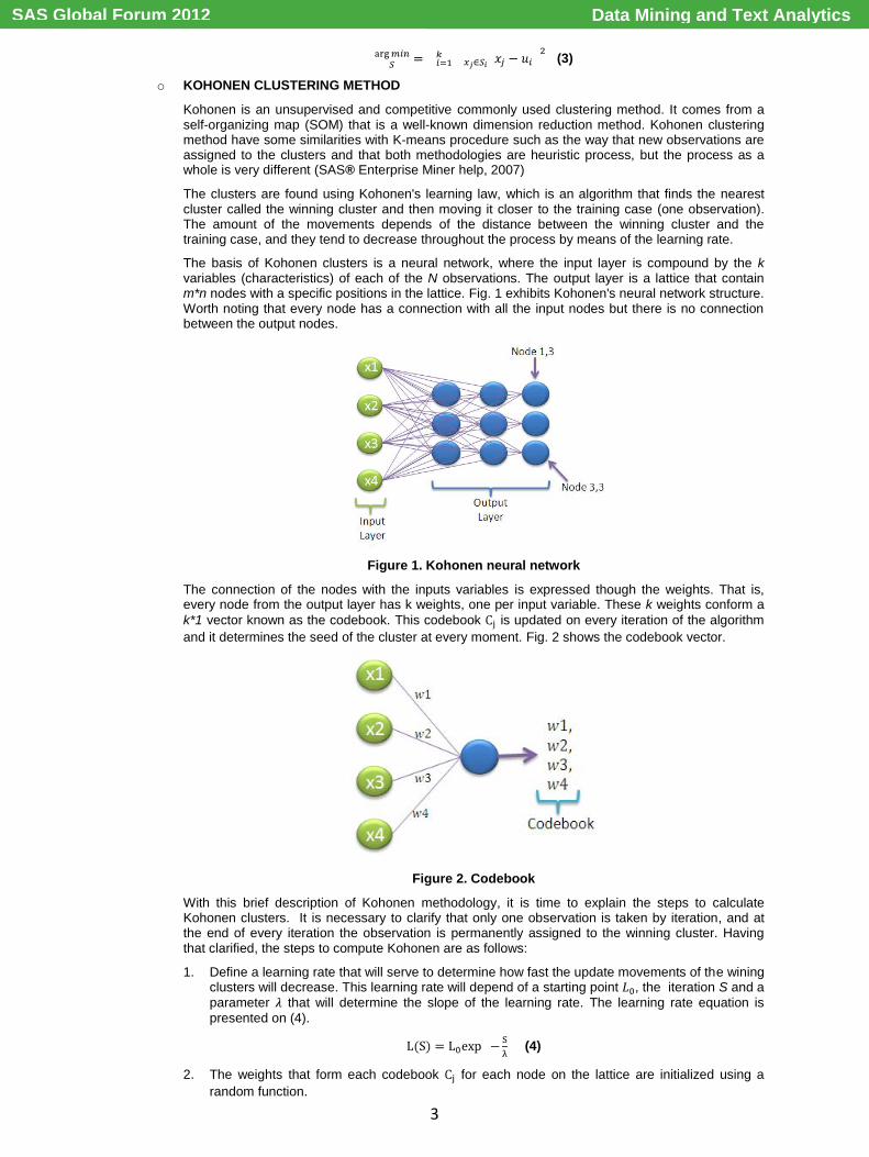
The basis of Kohonen clusters is a neural network, where the input layer is compound by the k variables (characteristics) of each of the N observations. The output layer is a lattice that contain m*n nodes with a specific positions in the lattice. Fig. 1 exhibits Kohonen's neural network structure. Worth noting that every node has a connection with all the input nodes but there is no connection between the output nodes.

Figure 1. Kohonen neural network

The connection of the nodes with the inputs variables is expressed though the weights. That is, every node from the output layer has k weights, one per input variable. These k weights conform a

k*1 vector known as the codebook. This codebook is updated on every iteration of the algorithm

and it determines the seed of the cluster at every moment. Fig. 2 shows the codebook vector.

Figure 2. Codebook

With this brief description of Kohonen methodology, it is time to explain the steps to calculate Kohonen clusters. It is necessary to clarify that only one observation is taken by iteration, and at the end of every iteration the observation is permanently assigned to the winning cluster. Having that clarified, the steps to compute Kohonen are as follows:

1. Define a learning rate that will serve to determine how fast the update movements of the wining clusters will decrease. This learning rate will depend of a starting point , the iteration S and a

parameter that will determine the slope of the learning rate. The learning rate equation is

presented on (4).

(4)

2. The weights that form each codebook for each node on the lattice are initialized using a

random function.

Data Mining and Text AnalyticsSAS Global Forum 2012

4

3. One training case (one observation) is selected and the winning cluster is calculated for that

observation. The winning cluster will be determined using the distance function (5):

(5)

where is the training case for the observation i, is the seed of the cluster in the

iteration or step.

4. The seed of the winning cluster is updated with the distance from the training case to cluster seed. The update is made with equation (6):

(6)

where is the learning rate in the iteration. The seed for all the other no winning clusters will stay equal in that iteration.

5. Repeat steps 3 and 4 until the convergence criterion is reached. There are many convergence criterions, but the most commonly used are the number of iterations or a defined learning rate level.

LOGISTIC REGRESSION

Logistic regression is a technique used when there is a need to predict the probability of occurrence of an event. It is similar to a linear regression model in the way that it helps determining the relationship between the independent variables and the dependent variable, but it is adapted for models in which the dependent variable is dichotomous. The independent variables can be either interval or categorical.

It is called logistic regression because it uses the logistic function to fit the output values between zero and one, just like a probability (Allison,2003).

This method is widely used to develop credit risk scorecards in order to predict the probability of a customer having a good payment habit if a loan is granted.

Although there are other techniques that could increase the predictive power of the models, the logistic regression has two strong features in its favor: i) Simplicity on the model developments and ii) ease of interpretability.

MULTINOMIAL LOGISTIC REGRESSION

A Multinomial logistic regression is a generalization of the logistic regression given that the dependent variable is not restricted to two categories. This means that these kinds of models are useful to predict the probability of an outcome when the dependent variable is categorical with more than two possibilities. In this case, just as in the logistic regression the independent variables can be either interval or categorical.

The process consists in fitting a multinomial logit model for the full factorial model or for a specified model and the parameter estimation is done through an iterative maximum likelihood algorithm (Allison,2003).

MULTI-LAYER PERCEPTRON NEURAL NETWORK

An artificial neural network is an abstraction of the real nervous system that consists of a collection of units called neurons that are highly interconnected with each other. An artificial neural network is composed by an input layer, a hidden layer and an output layer. Each layer is in turn composed by neural units (nodes). These units compute a value based on the sum of the inputs and then this value is propagated through the unidirectional connections to the other units of the network until the output layer is reached. The output layer computes for the final result of the process. In Addition, each of the connections of the network has an associated weight that is calculated by an iterative process (Rosenblatt, 1962).

The network discussed in this paper is called a Multi-Layer Perceptron neural network (MLP) and is described generally below. It has an input layer that represents the input variables to be used in the neural network model and it can be connected directly with the output layer. It also has i hidden layers and each layer contains j hidden units. The hidden units have a variety of hidden activation functions and a linear combination function. Finally, the MLP has an output layer that has a target activation function. Both, the hidden layers and the output layer could have the bias option activated. A bias term can be treated as a connection weight from a special unit with a constant, nonzero activation value. The term "bias" is usually used with respect to a "bias unit" with a constant value of one. For further information regarding the usage of an MLP neural network on credit scoring, please refer to Correa, Gonzalez and Ladino (2011).

CLASIFICATION DISTANCES

As will be explained in detail further in this paper, the MLP neural networks and the multinomial logistic regression techniques are used to classify a new client to a corresponding cluster. Also a distance

Data Mining and Text AnalyticsSAS Global Forum 2012

5

algorithm is used for the same task. This algorithm is based on the idea behind K-means, were each new client is assigned to the cluster with the minimum distance to it.

For this matter we used three different distance algorithms: minimum Euclidian distance, minimum adjusted distance and Mahalanobis distance.

o MINIMUM EUCLIDIAN DISTANCE

The minimum Euclidian distance attempts to assign a client to a cluster based on the distances of the client with the centroid of each of the defined clusters. This distance is calculated as follows on equation (7):

(7)

where (X,Y) is the coordinate of the client in the N dimensional space, and (Xc,Yc) are the coordinates of the centroid of each cluster.

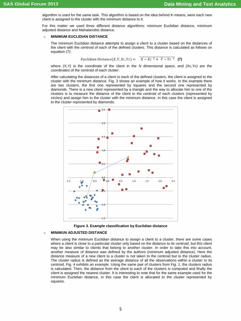
After calculating the distances of a client to each of the defined clusters, the client is assigned to the cluster with the minimum distance. Fig. 3 shows an example of how it works. In the example there are two clusters, the first one represented by squares and the second one represented by diamonds. There is a new client represented by a triangle and the way to allocate him to one of the clusters is to measure the distance of the client to the centroid of each clusters (represented by circles) and assign him to the cluster with the minimum distance. In this case the client is assigned to the cluster represented by diamonds.

Figure 3. Example classification by Euclidian distance

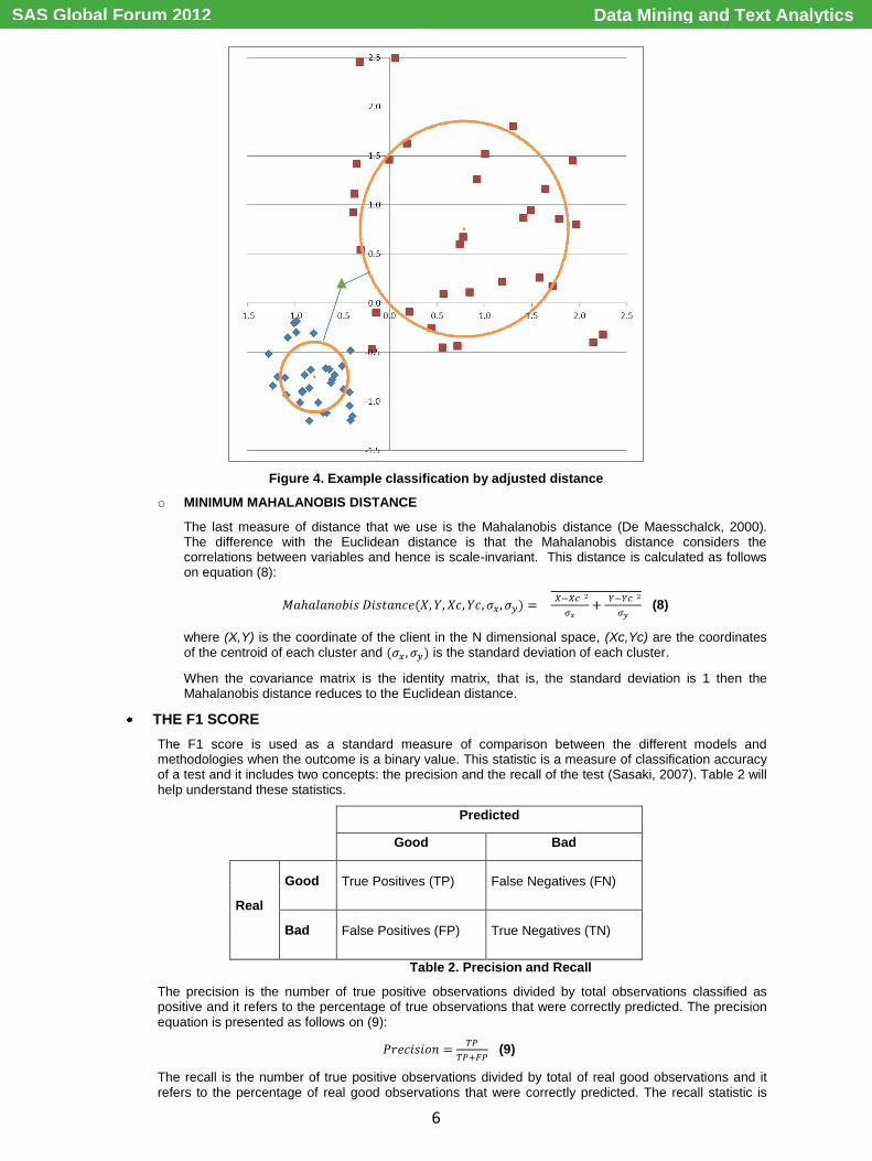
o MINIMUN ADJUSTED DISTANCE

When using the minimum Euclidian distance to assign a client to a cluster, there are some cases where a client is close to a particular cluster only based on the distance to its centroid, but this client may be also similar to clients that belong to another cluster. In order to take this into account, another measure of distance was defined by the authors (minimum adjusted distance). Here the distance measure of a new client to a cluster is not taken to the centroid but to the cluster radius. The cluster radius is defined as the average distance of all the observations within a cluster to its centroid. Fig. 4 exhibits an example. Using the same pair of clusters from Fig. 1, the clusters radius is calculated. Then, the distance from the client to each of the clusters is computed and finally the client is assigned the nearest cluster. It is interesting to note that for the same example used for the minimum Euclidian distance, in this case the client is allocated to the cluster represented by squares.

-1.5

-1.0

-0.5

0.0

0.5

1.0

1.5

2.0

2.5

-1.5 -1.0 -0.5 0.0 0.5 1.0 1.5 2.0 2.5

Data Mining and Text AnalyticsSAS Global Forum 2012

6

Figure 4. Example classification by adjusted distance

o MINIMUM MAHALANOBIS DISTANCE

The last measure of distance that we use is the Mahalanobis distance (De Maesschalck, 2000). The difference with the Euclidean distance is that the Mahalanobis distance considers the correlations between variables and hence is scale-invariant. This distance is calculated as follows on equation (8):

(8)

where (X,Y) is the coordinate of the client in the N dimensional space, (Xc,Yc) are the coordinates of the centroid of each cluster and is the standard deviation of each cluster.

When the covariance matrix is the identity matrix, that is, the standard deviation is 1 then the Mahalanobis distance reduces to the Euclidean distance.

THE F1 SCORE

The F1 score is used as a standard measure of comparison between the different models and methodologies when the outcome is a binary value. This statistic is a measure of classification accuracy of a test and it includes two concepts: the precision and the recall of the test (Sasaki, 2007). Table 2 will help understand these statistics.

Predicted

Good Bad

Real

Good True Positives (TP) False Negatives (FN)

Bad False Positives (FP) True Negatives (TN)

Table 2. Precision and Recall

The precision is the number of true positive observations divided by total observations classified as positive and it refers to the percentage of true observations that were correctly predicted. The precision equation is presented as follows on (9):

(9)

The recall is the number of true positive observations divided by total of real good observations and it refers to the percentage of real good observations that were correctly predicted. The recall statistic is

Data Mining and Text AnalyticsSAS Global Forum 2012

7

computed as follows on (10):

(10)

After calculating the values for the precision and the recall, the F1 score statistic can be calculated. The F1 score rake values between cero and one, being one the best score and cero the worst. The F1 score formula is presented on (11):

(11)

This formula stands for the harmonic mean between the precision and the recall statistics (Sasaki, 2007).

MODELING PROCESS

Now that the general concepts have been explained, in this stage we will focus on the modeling process undertaken to determine the most efficient and optimal way to select the best methodology for the predictive cluster analysis. Fig. 5 illustrates the process which is applied to each of the four databases.

Figure 5. Modeling process flowchart

Initially two kinds of cluster methodologies are used in order to segment the population in K defined groups. The two methodologies used for this purpose are K-means clustering and Kohonen SOM. Given that the resulting clusters are the inputs for the credit risk scorecards, it was important to define a minimum quantity of good and bad clients within each cluster, necessaries to be able to develop a model. For this case, the minimum number was set to 1.000 good and bad clients (Mays, 1998).

After obtaining the resulting clusters, the next step is to determine the probability that a new client belongs to one of the particular clusters. Therefore, a predictive model is developed by setting the clusters as the dependent variables and assigning them values between one and K depending on the number of clusters. In this step, five different ways of assigning a new client to a cluster are developed using the following methodologies: logistic regression, neural network (MLP), minimum Euclidian distance, minimum adjusted distance and Mahalanobis distance.

The third step is to develop a credit risk scorecard for each of the resulting clusters. To do this, two methodologies are used, logistic regression and MLP neural network. For this case of study the credit risk scorecards are built using the same methodology. This means that for a model with n clusters, all the n credit risk scorecards are going to be developed using only one of the two methodologies.

Finally, there is the definition of the final score that will classify the new clients as good or bad. In order to determine whether a client is good or bad based on the resulting probability, the statistical cut-off methodology is used for every final score (Mays, 2004).

The three different methodologies used in this phase are cluster score, score ensemble and classifier ensemble.

Cluster score: In this method the final score is the logistic regression or the neural network score developed for each resulting cluster in the previous step. That is, if a client is assigned to a cluster, then the credit risk score built for that specific cluster determines if the client is good or bad.

Ensemble score: This method takes into account all the scores defined for each of the clusters and the probability of the new client to belong to every cluster. Therefore the final score is the weighted average of the credit risk scores of the resulting clusters, weighted by the probability of belonging to each of them. Not for all the predictive clusters techniques the probability of belonging to a cluster is obtained straight forward. For the logistic regression and the MLP neural networks the output is already a probability, but for the distance techniques it is necessary to make a conversion given that the output of is a distance measure. To turn the resulting distance into a probability, the following equation (12) is used:

Data Mining and Text AnalyticsSAS Global Forum 2012

8

(12)

Classifier average vote ensemble: This method also takes into account all the scores of the resulting clusters and the final score is the consequence of the vote of each of the credit risk score, also weighted by the probability of belonging to each of them. This means that for every new client each of the credit risk scores developed for a specific cluster determines individually if the client is good or bad, and this dichotomous result (not the probability) is weighted by the probability of belonging to the clusters. This method is similar to the combination method used in ensemble models called majority voting (Hastie et al., 2003). Here, the conversion equation presented in the preceding paragraph is also used.

Beside the predictive clustering process, also a logistic regression model and a MLP neural network model are calculated for the entire population in order to use them as benchmark models and also the F1 Score is calculated for every model as is the measure of comparison which will be used between models.

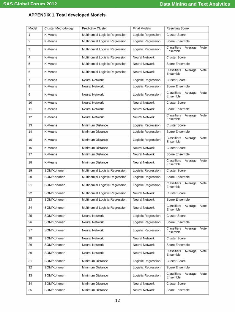
The complete process is made using SAS® base and SAS Enterprise Miner™ procedures inside different proprietary macros designed to optimize the complex process of developing 62 different the models for each of the four databases. In Appendix 1 there is a detailed list of the 62 developed models.

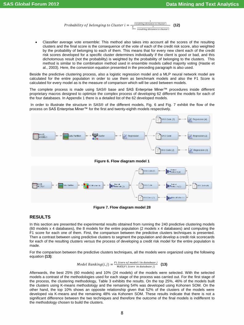
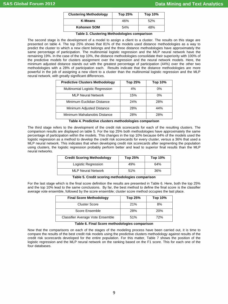
In order to illustrate the structure in SAS® of the different models, Fig. 6 and Fig. 7 exhibit the flow of the process on SAS Enterprise Miner™ for the first and twenty-eighth models respectively.

Figure 6. Flow diagram model 1

Figure 7. Flow diagram model 28

RESULTS

In this section are presented the experimental results obtained from running the 240 predictive clustering models (60 models x 4 databases), the 8 models for the entire population (2 models x 4 databases) and computing the F1 score for each one of them. First, the comparison between the predictive clusters techniques is presented. Then a contrast between using predictive clusters to segment the population and develop a credit risk scorecards for each of the resulting clusters versus the process of developing a credit risk model for the entire population is made.

For the comparison between the predictive clusters techniques, all the models were organized using the following equation (13):

(13)

Afterwards, the best 25% (60 models) and 10% (24 models) of the models were selected. With the selected models a contrast of the methodologies used for each stage of the process was carried out. For the first stage of the process, the clustering methodology, Table 3 exhibits the results. On the top 25%, 46% of the models built the clusters using K-means methodology and the remaining 54% was developed using Kohonen SOM. On the other hand, the top 10% shows an opposite relationship given that 52% of the clusters of the models were developed via K-means and the remaining 48% via Kohonen SOM. These results indicate that there is not a significant difference between the two techniques and therefore the outcome of the final models is indifferent to the methodology chosen to build the clusters.

Data Mining and Text AnalyticsSAS Global Forum 2012

9

Clustering Methodology Top 25% Top 10%

K-Means 46% 52%

Kohonen SOM 54% 48%

Table 3. Clustering Methodologies comparison

The second stage is the development of a model to assign a client to a cluster. The results on this stage are presented on table 4. The top 25% shows that 81% of the models used distance methodologies as a way to predict the cluster to which a new client belongs and the three distance methodologies have approximately the same percentage of participation. The multinomial logistic regression and the MLP neural network have the remaining 19%. In the case of the top 10%, the distance methodologies consolidate their superiority with 100% of the predictive models for clusters assignment over the regression and the neural network models. Here, the minimum adjusted distance stands out with the greatest percentage of participation (44%) over the other two methodologies with a 28% of participation each. Results indicate that the distance methodologies are more powerful in the job of assigning a new client to a cluster than the multinomial logistic regression and the MLP neural network, with greatly significant differences.

Predictive Clusters Methodology Top 25% Top 10%

Multinomial Logistic Regression 4% 0%

MLP Neural Network 15% 0%

Minimum Euclidian Distance 24% 28%

Minimum Adjusted Distance 28% 44%

Minimum Mahalanobis Distance 28% 28%

Table 4. Predictive clusters methodologies comparison

The third stage refers to the development of the credit risk scorecards for each of the resulting clusters. The comparison results are displayed on table 5. For the top 25% both methodologies have approximately the same percentage of participation within the models. This changes in the top 10% because 64% of the models used the logistic regression as a method to develop the credit risk scorecards for every cluster, versus a 36% that used a MLP neural network. This indicates that when developing credit risk scorecards after segmenting the population using clusters, the logistic regression probably perform better and lead to superior final results than the MLP neural networks.

Credit Scoring Methodology Top 25% Top 10%

Logistic Regression 49% 64%

MLP Neural Network 51% 36%

Table 5. Credit scoring methodologies comparison

For the last stage which is the final score definition the results are presented in Table 6. Here, both the top 25% and the top 10% lead to the same conclusions. By far, the best method to define the final score is the classifier average vote ensemble, followed by the score ensemble; cluster score method occupies the last place.

Final Score Methodology Top 25% Top 10%

Cluster Score 21% 8%

Score Ensemble 28% 20%

Classifier Average Vote Ensemble 51% 72%

Table 6. Final Score methodologies comparison

Now that the comparisons on each of the stages of the modeling process have been carried out, it is time to compare the results of the best credit risk models using the predictive clusters methodology against results of the credit risk scorecards developed for the entire population. For this matter, Table 7 shows the position of the logistic regression and the MLP neural network on the ranking based on the F1 score. This for each one of the four databases.

Data Mining and Text AnalyticsSAS Global Forum 2012

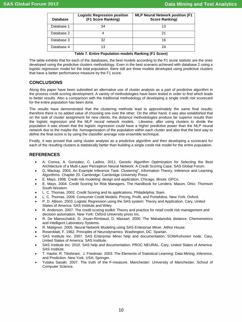
10

Database Logistic Regression position

(F1 Score Ranking) MLP Neural Network position (F1

Score Ranking)

Database 1 34 13

Database 2 4 21

Database 3 32 16

Database 4 13 24

Table 7. Entire Population models Ranking (F1 Score)

The table exhibits that for each of the databases, the best models according to the F1 score statistic are the ones developed using the predictive clusters methodology. Even in the best scenario achieved with database 2 using a logistic regression model for the total population, there still are three models developed using predictive clusters that have a better performance measure by the F1 score.

CONCLUSIONS

Along this paper have been submitted an alternative use of cluster analysis as a part of predictive algorithm in the process credit scoring development. A variety of methodologies have been tested in order to find which leads to better results. Also a comparison with the traditional methodology of developing a single credit risk scorecard for the entire population has been done.

The results have demonstrated that the clustering methods lead to approximately the same final results; therefore there is no added value of choosing one over the other. On the other hand, it was also established that on the task of cluster assignment for new clients, the distance methodologies produce far superior results than the logistic regression and the MLP neural network models. Likewise, after using clusters to divide the population it was shown that the logistic regression could have a higher predictive power than the MLP neural network due to the maybe the homogenization of the population within each cluster and also that the best way to define the final score is by using the classifier average vote ensemble technique.

Finally, it was proved that using cluster analysis as a predictive algorithm and then developing a scorecard for each of the resulting clusters is statistically better than building a single credit risk model for the entire population.

REFERENCES

A. Correa, A. Gonzalez, C. Ladino. 2011. Genetic Algorithm Optimization for Selecting the Best Architecture of a Multi-Layer Perceptron Neural Network: A Credit Scoring Case. SAS Global Forum.

D, Mackay. 2003. An Example Inference Task: Clustering". Information Theory, Inference and Learning Algorithms. Chapter 20. Cambridge: Cambridge University Press.

E. Mays. 1998. Credit risk modeling: design and application. Chicago, illinois: GPCo.

E. Mays. 2004. Credit Scoring for Risk Managers. The Handbook for Lenders. Mason, Ohio: Thomson South-Western.

L. C. Thomas. 2002. Credit Scoring and its applications. Philadelphia: Siam.

L. C. Thomas. 2009. Consumer Credit Models: Pricing, Profit, and Portafolios. New York: Oxford.

P. D. Allison. 2003. Logistic Regression using the SAS system: Theory and Application. Cary, United States of America: SAS Institute and Wiley.

R. Anderson. 2007. The credit scoring toolkit: Theory and practice for retail credit risk management and decision automation. New York: Oxford University press Inc.

R. De Maesschalck, D. Jouan-Rimbaud, D. Massart. 2000. The Mahalanobis distance. Chemometrics and Intelligent Laboratory Systems.

R. Matignon. 2005. Neural Network Modeling using SAS Enterprise Miner. Aithor House.

Rosenblatt, F. 1962. Principles of Neurodynamics. Washington, DC: Spartan.

SAS Institute Inc. 2007. SAS Enterprise Miner help and documentation, SOM/Kohonen node. Cary, United States of America: SAS Institute.

SAS Institute Inc. 2010. SAS help and documentation, PROC NEURAL. Cary, United States of America: SAS Institute.

T. Hastie, R. Tibshirani, J. Friedman. 2003. The Elements of Statistical Learning: Data Mining, Inference, and Prediction. New York, USA: Springer.

Yutaka Sasaki. 2007. The truth of the F-measure. Manchester: University of Manchester, School of Computer Science.

Data Mining and Text AnalyticsSAS Global Forum 2012

11

CONTACT INFORMATION Your comments and questions are valued and encouraged. Contact the authors at:

Name: Alejandro Correa Bahnsen Enterprise: Banco Colpatria City: Bogotá, Colombia Phone: (+57) 3208306606 E-mail: al.bahnsen@gmail.com Name: Andrés González Enterprise: Banco Colpatria City: Bogotá, Colombia Phone: (+57) 3103595239 E-mail: correaal@colpatria.com Name: Catherine Nieto Enterprise: Banco Colpatria City: Bogotá, Colombia Phone: (+57) 3157426533 E-mail: nietoa@colpatria.com Name: Darwin Amezquita Enterprise: Banco Colpatria City: Bogotá, Colombia Phone: (+57) 3013372763 E-mail: amezqud@colpatria.com

SAS and all other SAS Institute Inc. product or service names are registered trademarks or trademarks of SAS Institute Inc. in the USA and other countries. ® indicates USA registration. Other brand and product names are trademarks of their respective companies.

Data Mining and Text AnalyticsSAS Global Forum 2012

12

APPENDIX 1. Total developed Models

Model Cluster Methodology Predictive Cluster Final Models Resulting Score

1 K-Means Multinomial Logistic Regression Logistic Regression Cluster Score

2 K-Means Multinomial Logistic Regression Logistic Regression Score Ensemble

3 K-Means Multinomial Logistic Regression Logistic Regression Classifiers Average Vote Ensemble

4 K-Means Multinomial Logistic Regression Neural Network Cluster Score

5 K-Means Multinomial Logistic Regression Neural Network Score Ensemble

6 K-Means Multinomial Logistic Regression Neural Network Classifiers Average Vote Ensemble

7 K-Means Neural Network Logistic Regression Cluster Score

8 K-Means Neural Network Logistic Regression Score Ensemble

9 K-Means Neural Network Logistic Regression Classifiers Average Vote Ensemble

10 K-Means Neural Network Neural Network Cluster Score

11 K-Means Neural Network Neural Network Score Ensemble

12 K-Means Neural Network Neural Network Classifiers Average Vote Ensemble

13 K-Means Minimum Distance Logistic Regression Cluster Score

14 K-Means Minimum Distance Logistic Regression Score Ensemble

15 K-Means Minimum Distance Logistic Regression Classifiers Average Vote Ensemble

16 K-Means Minimum Distance Neural Network Cluster Score

17 K-Means Minimum Distance Neural Network Score Ensemble

18 K-Means Minimum Distance Neural Network Classifiers Average Vote Ensemble

19 SOM/Kohonen Multinomial Logistic Regression Logistic Regression Cluster Score

20 SOM/Kohonen Multinomial Logistic Regression Logistic Regression Score Ensemble

21 SOM/Kohonen Multinomial Logistic Regression Logistic Regression Classifiers Average Vote Ensemble

22 SOM/Kohonen Multinomial Logistic Regression Neural Network Cluster Score

23 SOM/Kohonen Multinomial Logistic Regression Neural Network Score Ensemble

24 SOM/Kohonen Multinomial Logistic Regression Neural Network Classifiers Average Vote Ensemble

25 SOM/Kohonen Neural Network Logistic Regression Cluster Score

26 SOM/Kohonen Neural Network Logistic Regression Score Ensemble

27 SOM/Kohonen Neural Network Logistic Regression Classifiers Average Vote Ensemble

28 SOM/Kohonen Neural Network Neural Network Cluster Score

29 SOM/Kohonen Neural Network Neural Network Score Ensemble

30 SOM/Kohonen Neural Network Neural Network Classifiers Average Vote Ensemble

31 SOM/Kohonen Minimum Distance Logistic Regression Cluster Score

32 SOM/Kohonen Minimum Distance Logistic Regression Score Ensemble

33 SOM/Kohonen Minimum Distance Logistic Regression Classifiers Average Vote Ensemble

34 SOM/Kohonen Minimum Distance Neural Network Cluster Score

35 SOM/Kohonen Minimum Distance Neural Network Score Ensemble

Data Mining and Text AnalyticsSAS Global Forum 2012

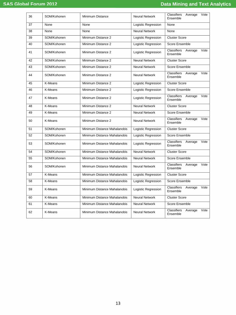
13

36 SOM/Kohonen Minimum Distance Neural Network Classifiers Average Vote Ensemble

37 None None Logistic Regression None

38 None None Neural Network None

39 SOM/Kohonen Minimum Distance 2 Logistic Regression Cluster Score

40 SOM/Kohonen Minimum Distance 2 Logistic Regression Score Ensemble

41 SOM/Kohonen Minimum Distance 2 Logistic Regression Classifiers Average Vote Ensemble

42 SOM/Kohonen Minimum Distance 2 Neural Network Cluster Score

43 SOM/Kohonen Minimum Distance 2 Neural Network Score Ensemble

44 SOM/Kohonen Minimum Distance 2 Neural Network Classifiers Average Vote Ensemble

45 K-Means Minimum Distance 2 Logistic Regression Cluster Score

46 K-Means Minimum Distance 2 Logistic Regression Score Ensemble

47 K-Means Minimum Distance 2 Logistic Regression Classifiers Average Vote Ensemble

48 K-Means Minimum Distance 2 Neural Network Cluster Score

49 K-Means Minimum Distance 2 Neural Network Score Ensemble

50 K-Means Minimum Distance 2 Neural Network Classifiers Average Vote Ensemble

51 SOM/Kohonen Minimum Distance Mahalanobis Logistic Regression Cluster Score

52 SOM/Kohonen Minimum Distance Mahalanobis Logistic Regression Score Ensemble

53 SOM/Kohonen Minimum Distance Mahalanobis Logistic Regression Classifiers Average Vote Ensemble

54 SOM/Kohonen Minimum Distance Mahalanobis Neural Network Cluster Score

55 SOM/Kohonen Minimum Distance Mahalanobis Neural Network Score Ensemble

56 SOM/Kohonen Minimum Distance Mahalanobis Neural Network Classifiers Average Vote Ensemble

57 K-Means Minimum Distance Mahalanobis Logistic Regression Cluster Score

58 K-Means Minimum Distance Mahalanobis Logistic Regression Score Ensemble

59 K-Means Minimum Distance Mahalanobis Logistic Regression Classifiers Average Vote Ensemble

60 K-Means Minimum Distance Mahalanobis Neural Network Cluster Score

61 K-Means Minimum Distance Mahalanobis Neural Network Score Ensemble

62 K-Means Minimum Distance Mahalanobis Neural Network Classifiers Average Vote Ensemble

Data Mining and Text AnalyticsSAS Global Forum 2012