S T E A D Y O N E – D I M E N S I O N A L C O N V E C T I O N & D I F F U S I O

N

0

dx

ud

dx

d

dx

du

dx

d

x pe x w p

x w e

Ww

EP e

uw ue

we

we xA

xAuAuA

0 we uAuA

&

wp

ww xD

pE

ee xD

uF x

D

ww uF ee uF

wPwPEewwee DDFF

0 we FF

T H E C E N T R A L

D I F F E R E N C I N G S C H E M E

  

2/EPe

2/PWw

WPwPEePWw

Epe F

φφDφφDφφ2

φφ2

F

Ee

eWw

wpe

ew

w

FD

FD

FD

FD

2222

pwee

ew

w FFF

DF

D

22

Ee

eww

w

FD

FD

22

EEwwpp aaa

aw aE ap

2w

w

FD

2e

e

FD weEw FFaa

A property is transported by

means of convection and

diffusion through the one –

dimensional domain – sketched

in Figure 5.2.

F O R E N D N O D E A

AeAPA

pee

uuxx

e)()()(

2/)(

)(2)()(2 APApeeAApe DDFFe

AAPApeEEAAPe DDDDFFeFe 2222

Grouping the above equation in the form

ueewwPp saaa

AAAAeepAe DFFe

DDDFe 2)

2(0)2

2(

Now we have to re arrange ap in the form

pweewp SFFaaa )(

Let us add and subtract Fe / 2 and Fw in the term ap.

wwAep FFFeFe

DDFe

a 22

22

)]2[()()2

(0 wAweep FDFFFe

Da

The governing equation is

( 5.3 ), boundary

conditions are 0 = 1 at

x = 0 and L = 0 at x – L. Using

five equally spaced cells and the

central differencing scheme for

convection and diffusion

calculate the distribution of as a

function of x for

C a s e 1 :

u = 0.1 m / s,

C a s e 2 :

u = 2.5 m / s, and compare the results

with

the analytical Solution.C a s e 3 :

Recalculate the solution for u = 2.5 m / s

with 20 grid nodes and compare the

results with the analytical solution. The

following data apply: length L = 1.0 m.

= 1.0 kg / m3, = 0.1

kg / m / s

= 1 x = o

= o

x = L

x x

x

W w P e E

1 32 4 5A B

APAPEeAAEP DDF 2

Fe

wPwPBBWPw

BB DDF

F 2

C E N T R A L D I F F E R E N C E M E T H O D

N O D E - A

N O D E - B

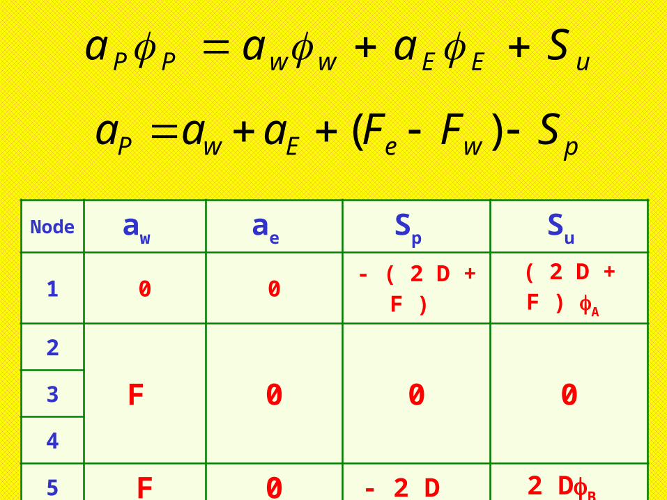
uEEwwpp Saaa

PweEWp SFFaaa

Node aw aE Sp Su

1 0 D - F / 2 - ( 2D + F ) ( 2 D + F ) A

2

D + F / 2 D - F / 2 0 03

4

5 D + F / 2 0 - ( 2D - F ) ( 2 D - F ) B

7183.1

)exp(7183.2 xx

0.2 0.4 0.6 0.80.0 1.0

Exact Solution

Numerical Solution ( CD )

1.0

0.8

0.6

0.4

0.2

D i s t a n c e ( m )

Numerical Solution ( CD )

Exact Solution

U = 2 . 5 m /s

101020.7

)25exp(11

x

xx

C A S E 2

0 . 0 0 . 2 0 . 4 0 . 6 0 . 8 1 . 0

Exact Solution

Numerical Solution ( C D )

U = 2 . 5 m /s

D i s t a n c e ( m )

1.0

0.8

0.6

0.4

0.2

P R O P E R T I E S O F

D I S C R E T I S A T I O N S C H E M E

S

• Conservativeness

• Boundedness

• Transportiveness

C O N S E R V A T I V E N E S

STo ensure conservation of for

the whole solution domain the

flux of leaving a control

volume across a certain face

must be equal to the flux of

entering the adjacent control

volume through the same face.

G r a d i e n t = (2 - 2 ) / x

x / 2 x x x x / 2

qA qB

1

23 4

1 2 3 4

C O N S I S T E N T S P E C I F I C A T I O N O F D I F F U S I V E F L U X E S

xx we

23

134

1

ABWB qq

xq

344

xxq

x weAe

12

223

212

1

I N C O N S I S T E N T S P E C I F I C A T I O N O F D I F F U S I V E F L U X E S

x / 2

x x x

x / 2

q B

1

23

4

1 2 3 4

Gradient of 2

Gradient of 2

Quadratic function 1

Quadratic function 2

q A

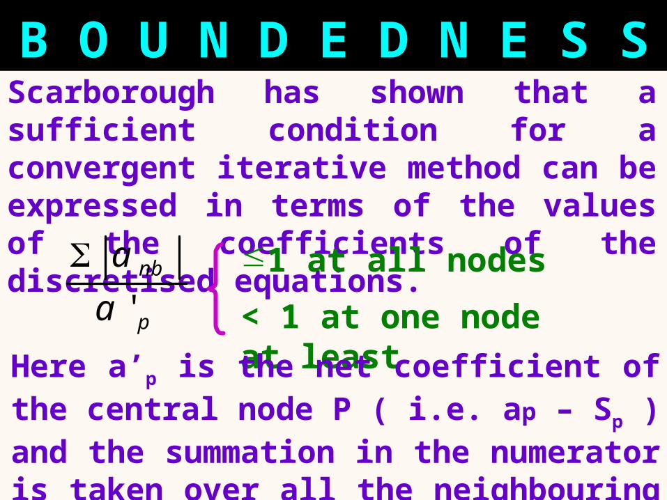
B O U N D E D N E S SScarborough has shown that a sufficient condition for a convergent iterative method can be expressed in terms of the values of the coefficients of the discretised equations.

p

nb

a

a

'

£1 at all nodes

< 1 at one node at least

Here a’p is the net coefficient of the central node P ( i.e. ap – Sp ) and the summation in the numerator is taken over all the neighbouring nodes ( nb ).

• Diagonal dominance is a desirable

feature

for satisfying the bounded ness

criterion.

This states that in the absence

of

sources the internal nodal values

of

the property should be bounded

by

its boundary values.

• All coefficients of the discretised

equations

should have the same sign ( usually all

positive )

T R A N S P O R T I V E N E S S

x

u

D

FPe

/

WP E

P e = 0

P e

Thus the value of at E is affected

only by upstream conditions and

since there is no diffusion E is

equal to P. It is very important

that the relationship between the

magnitude of the Peclet number

and the directionality of

influencing, known as the

transportiveness, is borne out in

the discretisation scheme.

aw aE aP

2w

w

FD

2e

e

FD )( weEw FFaa

I N T E R N A L C O E F F I C I E N T S O F D I S C R E T I S E D S C A L A R

T R A N S P O R T

2/ eee PeDF

U P W I N D D I F F E R E N C I N G S C H E M E W H E N I S P O S

I T I V E

xWw

xwP xPexeE

W W

Pe E

w w

P e

E

uw ue

Ww Pe &

)()( WPwPEeWwPe DDFF

EewwwPeew DFDFDD )()(

)89(31 EApAD

x

EeuEw DFD )(

U P W I N D D I F F E R E N C I N G S C H E M E W H E N I S N E GA T I V

E

w

xWw

xwP xPe xeE

W Pe E

w w P

e E

uw ue

Pw Ee )()( wPwPEePwEe DDFF

EeewwPweeew FDDFFFDD )()]()([

EEwwpp aaa

)( weEwp FFaaa

&

aw aE

Fw > 0, Fe > 0

Dw + Fw De

Fw < 0, Fe < 0

Dw De - Fe

aw aE

)0,max( ww FD ),0max( we FD

)()(:1 APAPEeAAPe DDFFNODE

)()(:5 wPwPBBWwPB DDFFNODE Node aw ae Sp Su

1 0 D- ( 2 D +

F ) ( 2 D + F )

A

2

D + F D 0 03

4

5 D + F 0 - 2 D 2 DB

U P W I N D S O L U T I O N T O S A M E P R O B L E M

The governing equation is

( 5.3 ), boundary

conditions are 0 = 1 at

x = 0 and L = 0 at x = L. Using

five equally spaced cells and the

central differencing scheme for

convection and diffusion

calculate the distribution of as a

function of x for

C a s e 1 :

u = 0.1 m / s,

C a s e 2 :

u = 2.5 m / s, and compare the results

with

the analytical Solution.C a s e 3 :

Recalculate the solution for u = 2.5 m / s

with 20 grid nodes and compare the

results with the analytical solution. The

following data apply: length L = 1.0 m.

= 1.0 kg / m3, = 0.1

kg / m / s

U P W I N D D I F F E R E N C I N G

S C H E M E

ueewwpp Saaa

Node

aw ae Sp Su

1 0 D – F / 2 - ( 2D + F ) ( 2D + F ) A

2,3,4 D + F / 2 D – F / 2 0 0

5 D + F / 2 0 - ( 2D - F ) ( 2D + F ) B

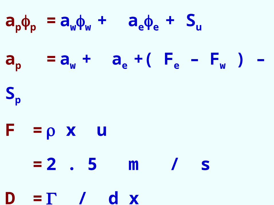
pweewp SFFaaa )(

F = x U

= 1 x 0 . 1

= 0 . 1

D = / x

= 0 . 1 / 0 . 2

= 0 . 5

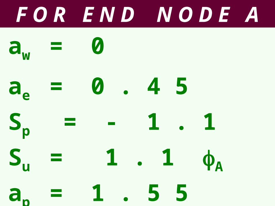
F O R E N D N O D E A

aw = 0

ae = 0 . 4 5

Sp = - 1 . 1

Su = 1 . 1 A

ap = 1 . 5 5

F O R I N T E R M E D I A T E N O D E S

aw = 0 . 5 5

ae = 0 . 4 5

Sp = 0

Su = 0

ap = 1

F O R E N D N O D E B

aw = 0 . 5 5

ae = 0

Sp = - 0 . 9

Su = 0 . 9 B

ap = aw +ae + ( Fe – Fw ) -

Sp

ap = 1 . 4 5

app = aw w + ae e + Su

1 . 55 p = 0 + 0 . 4 5 e + 1 .1

A

1p = 0 . 5 5 w + 0 . 4 5 e

p = 0 . 5 5 w + 0 . 4 5 e

p = 0 . 5 5 w + 0 . 4 5 e

1 . 4 5 p = 0 . 5 5 w + 0 . 9

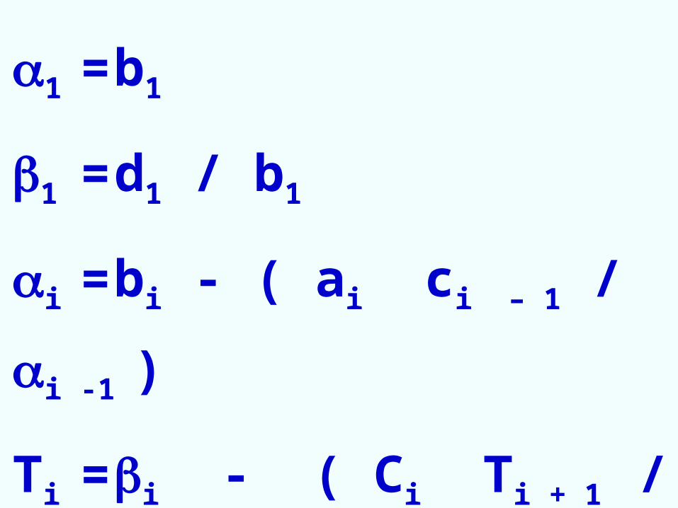
1 = b1

1 = d1 / b1

i = bi - ( ai ci – 1 / i -1 )

Ti = i - ( Ci Ti + 1 / i )

1 = ( di - ai i - 1 ) / i

1 = 1 . 5 5

1 = 0 . 7 0

2 = 0 . 8 4

3 = 0 . 7 0

4 = 0 . 6 5

5 = 1 . 0 6

2 = 0 . 4 5

3 = 0 . 3 5

4 = 0 . 2 9

5 = 0 . 1 5 0

T 5 = 5

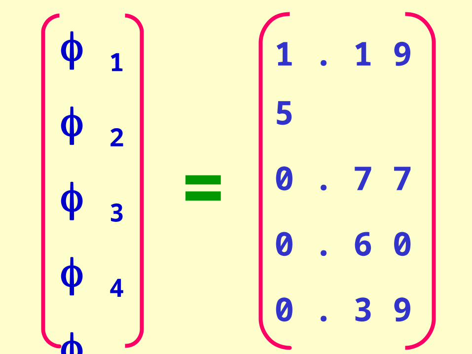
T 5 = 0 . 1 5 0

T 4 = 0 . 3 9

T 3 = 0 . 6 0

T 2 = 0 . 7 7

T 1 = 1 . 1 9 5

1

2

3

4

5

1 . 1 9

5

0 . 7 7

0 . 6 0

0 . 3 9

0 . 1 5

0

=

U P W I N D D I F F E R E N C I N G

S C H E M E ( U = 2.5

m /s )

ueewwpp Saaa

Node

aw ae Sp Su

1 0 D – F / 2 - ( 2D + F ) ( 2D + F ) A

2,3,4 D + F / 2 D – F / 2 0 0

5 D + F / 2 0 - ( 2D - F ) ( 2D + F ) B

pweewp SFFaaa )(

app = aww + aee + Su

ap = aw + ae +( Fe – Fw ) – Sp

F = x u

= 2 . 5 m / s

D = / d x

= 0 . 5

F O R E N D N O D E Aaw = 0

ae = D – F / 2

= - 0 . 7 5Sp = - ( 2 D + F )

= - 3 . 5Su = 3 . 5 A

ap = 2 . 7 5

F O R I N T E R M E D I A T E N O D E S

aw = D + F / 2

= 1 . 7 5

Qe = D - F / 2

= - 0 . 7 5

Sp = 0

ap = 1

F O R E N D N O D E B

aw = D + F / 2

= 1 . 7 5ae = 0

Sp = - ( 2 D - F )

= 1 . 5Su = ( 2 D – F ) B

= - 1 . 5 B

ap = 0 . 2 5

app = aw w + ae e + Su

2 . 7 5 p = - 0 . 7 5 e + 3 . 5

A

p = 1 . 7 5 w - 0 . 7 5 e

p = 1 . 7 5 w - 0 . 7 5 e

p = 1 . 7 5 w - 0 . 7 5 e

0 . 2 5 p = 1 . 7 5 w - 1 . 5

B

1 = b1

1 = d1 / b1

i = bi - ( ai ci – 1 / i -1 )

Ti = i - ( Ci Ti + 1 / i )

1 = ( di - ai I - 1 ) / i

1 = 2 . 7 5

1 = 1 . 2 7

2 = 1 . 4 8

3 = 1 . 8 8

4 = 1 . 6 9

5 = 1 . 0 2

2 = 1 . 5 0

3 = 1 . 4 0

4 = 1 . 4 5

5 = 2 . 4 8

T 5 = 5 = 2 . 4 8

T 4 = 0 . 3 4 9

T 3 = 1 . 2 6 0

T 2 = 0 . 8 6

T 1 = 1 . 0 3 5

T 4 = 0 . 3 4 9

T 3 = 1 . 2 6 0

T 2 = 0 . 8 6

T 1 = 1 . 0 3 5

1

2

3

4

5

1 . 0 3

5

0 . 8 6

1 . 2 6

0

0 . 3 4

9

2 . 4 8

=

N U M E R I C A L R E S U L T S &

A N A L Y T I C A L S O L U T I O N

0.0

0.2

0.4

0.6

0.8

1.0

0.2 0.4 0.6 0.8 1

Numerical Solution ( UD )

Exact Solution

U – 0.1 m / s

0.0

0.2

0.4

0.6

0.8

1.0

1.2

0.2 0.4 0.6 0.8 1.0

Distance ( m )

N U M E R I C A L R E S U L T S &

A N A L Y T I C A L S O L U T I O N

Numerical Solution ( UD )

Exact Solution

U = 2 . 5 m / s

F L O W D O M A I N F O R T H E I L L U S T R A T I O N O F F A L S E D I F F U S I O

N

= 0

= 1 0 0

=

1 0

0

=

0

V =

2 m

/ s

U = 2 m / s

X

X

H Y B R I D D I F F E R E N C I N G

S C H E M E

WPw

w

w

ww x

u

D

FPe

/

)(

P

wW

www PPFq

e

21

2

1

e

21

2

1

22 Pefor

2

Pe

forAFq Pwww

EEwwPP aaa

)( weEwP FFaaa

2

Pe

forAFq wwww

aw aE

0,

2max ,

www

FDF

0,

2,max e

ee

FDF

)(0 APAAAPe DFF

0)( PBBwwPB DFF

uEEwwPP Saaa

pweEwP SFFaaa )(

Node aw ae Sp Su

1 0 0- ( 2 D +

F ) ( 2 D + F )

A

2

F 0 0 03

4

5 F 0 - 2 D 2 DB

0.6

0.2 0.4 0.6 0.80.0

1.0

Numerical Solution( Hybrid, 25 cells )

Numerical Solution( Hybrid, 5 cells )

U – 2.5 m /s

Distance ( m )

Exact Solution0.2

0.4

0.8

0.0

)rrBBNNssEEwwPP aaaaaaa Faaaaaaa TBNsEwP

One – dimensional flow

Two - dimensional

flow

Three – dimensional flow

aw

aE

as

-aN

aB -

ar

F

0,

2,max w

ww

FDF

0,

2,max w

ww

FDF

0,

2,max e

ee

FDF

0,

2,max s

ss

FDF

0,

2,max n

nn

FDF

0,

2,max w

ww

FDF

0,

2,max e

ee

FDF

0,

2,max s

ss

FDF

0,

2,max n

nn

FDF

0,

2,max t

tt

FDF

we FF snwe FFFF btsnwe FFFFFF

0,

2,max b

bb

FDF

0,

2,max e

we

FDF

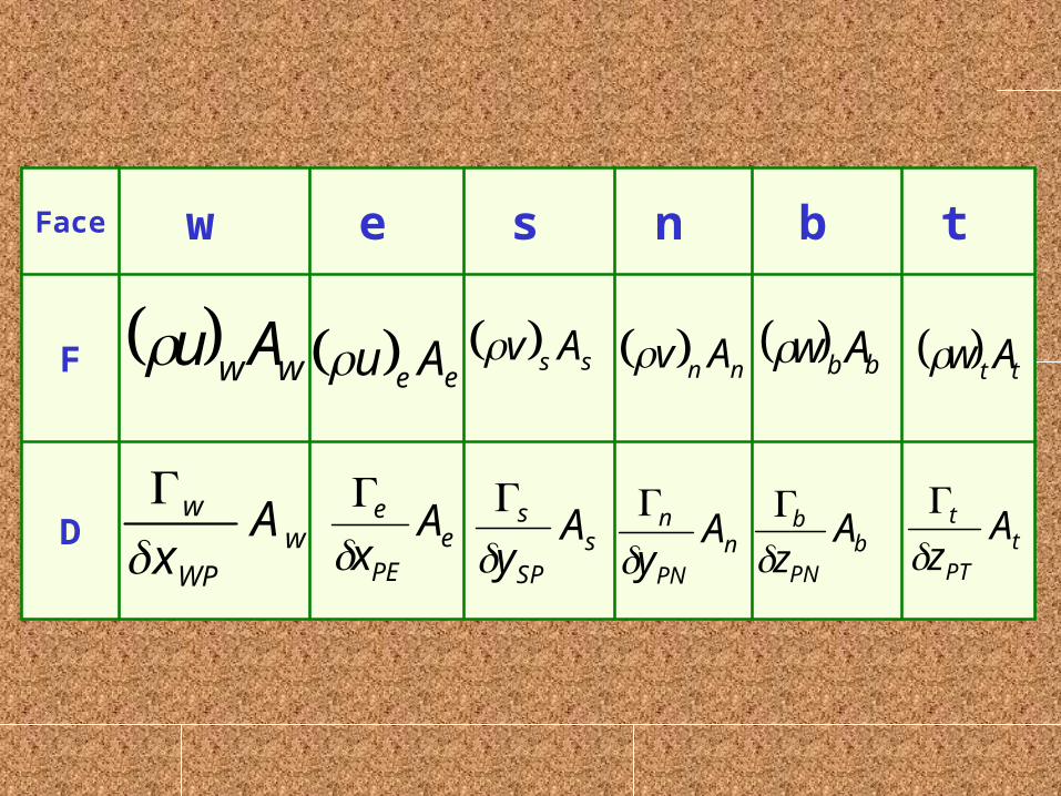
Face w e s n b t

F

D

ww Au

wWP

w Ax

ee Au

ePE

e Ax

ss Av

sSP

s Ay

nn Av

nPN

n Ay

bb Aw

bPN

b Az

tt Aw

tPT

t Az

P O W E R – L A W S C H E M E 100)]([ PeforFq wPwwww

www Fq f o r P e > 1 0

)( weEwP FFaaa

aw aE

]0,max[/)/1.01(,max 5www FPeOD ]0,max[/)/1.01(,max 5

eee FPeOD

W = ( 1 – 0.1 Pew ) 5 / Pew

Q U A D R A T I C P R O F I L E S U S E D

I N T H E Q U I C K S C H E M E

WW W w P e E EE

EE W

w

pe E

WW

21 8

1

8

3

8

6 iiiface

WWpWw 8

1

8

3

8

6

WEpe 8

1

8

3

8

6

WWPWwWEPe FF

8

1

8

3

8

6

8

1

8

3

8

6

)()( wpwpEe DD

Wewwpeeww FFDFDFD

8

1

8

6

8

6

8

3

WWwEee FFD 8

1

8

3

wwwwEEwwPP aaaa

aw aE aww ap

eww FFD8

1

8

6

ee FD8

3 eF8

1 )( wewwEw FFaaa

aw aE aEE ap

EWPw 8

1

8

3

8

6

EEpEe 8

1

8

3

8

6

ww FD8

3 Wee FFD

8

1

8

6

eF8

1 )( weEEEw FFaaa

EEEEWWWWEEwwPP aaaaa

)( weEEWWEwP FFaaaaa

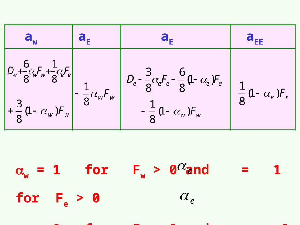
aw aE aE aEE

eewww FFD 8

1

8

6

wwF8

1

eeeee FFD )1(8

6

8

3

ww F)1(8

1 ee F)1(

8

1

ww F)1(8

3

w = 1 for Fw > 0 and = 1 for Fe >

0

w = 0 for Fw < 0 and = 0 for Fe <

0

e

e

M I R R O R N O D E T R E A T M E N T

A T T H E B O U N D A R Y

0

A

p

x / 2 x / 2

Mirror Node

Domain Boundary

Node 1

0 P

pAo 2

)2(8

1

8

3

8

6pAEpe

AEpe 8

2

8

3

8

7

)89(31 EApAD

x

)89(3

)(8

2

8

3

8

7EAp

ApEeAAAEpe

DDFF

)98(3 wPBB

B

D

x

wwpwwBB FF

8

1

8

3

8

6

)()98(3 wpwwpBB DD

ApwwwEpe FF

8

2

8

3

8

7

8

1

8

3

8

6

)()( wpwpEe DD

uEEwwwwwwpp Saaaa

pweEwwwp SFFaaaa )(

The governing equation is

( 5.3 ), boundary

conditions are 0 = 1 at

x = 0 and L = 0 at x = L. Using

five equally spaced cells and the

central differencing scheme for

convection and diffusion

calculate the distribution of as a

function of x for

C a s e 1 :

u = 0.1 m / s,

C a s e 2 :

u = 2.5 m / s, and compare the results

with

the analytical Solution.C a s e 3 :

Recalculate the solution for u = 2.5 m / s

with 20 grid nodes and compare the

results with the analytical solution. The

following data apply: length L = 1.0 m.

= 1.0 kg / m3, = 0.1

kg / m / s

= 1 x = o

= o

x = L

x x

x

W w P e E

1 32 4 5A B

H Y B R I D S C H E M E

uEEwwPP Saaa

pweEwP SFFaaa )(

Node aw ae Sp Su

1 0 0- ( 2 D +

F ) ( 2 D + F )

A

2

F 0 0 03

4

5 F 0 - 2 D 2 DB

)(0 ApAAApe DFF

0)( pBBwwpB DFF

Suaaa eewwpp

pweewp SFFaaa )(

F = x u

= 2 . 5

D = / d x

= 0 . 5

P e = u / ( / x )

= 5

If Pe > 2, Hybrid Scheme uses

Upwind Expression for Convection

term & Set Diffusion Term to

Zero

)(0 ApAAApe DFF

0)( pBBwwpB DFF

N O D E - 1

N O D E - 5

Suaaa eewwpp

pweewp SFFaaa )(

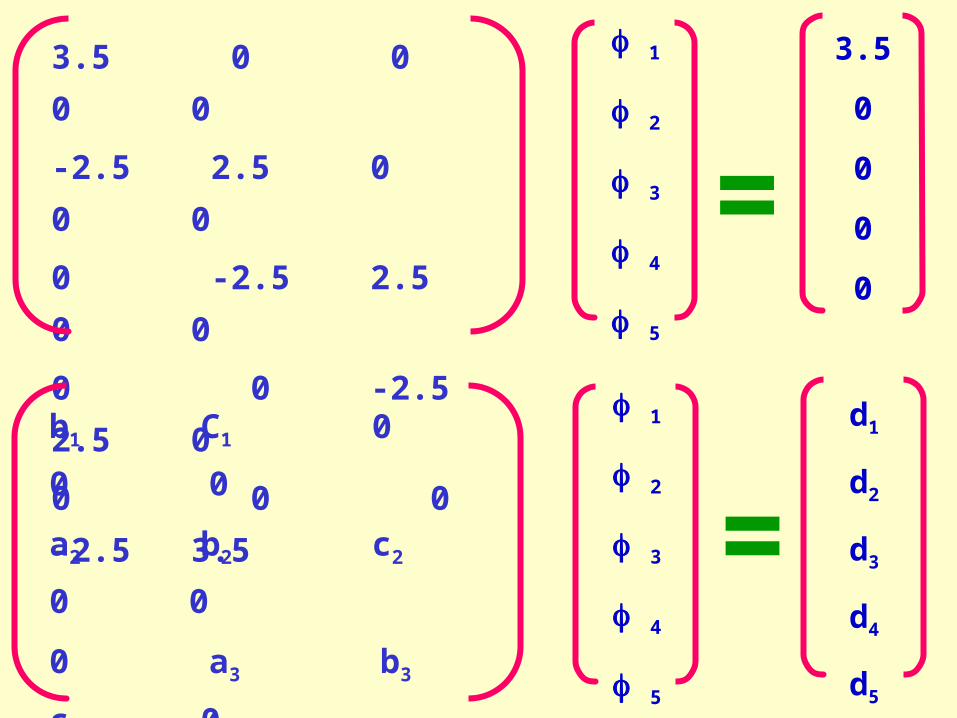
3.5 0 0 0 0

-2.5 2.5 0 0 0

0 -2.5 2.5 0 0

0 0 -2.5 2.5 0

0 0 0 -2.5

3.5

1

2

3

4

5

3.5

0

0

0

0

=

b1 C1 0 0 0

a2 b2 c2 0 0

0 a3 b3 c3 0

0 0 a4 b4 c4

0 0 0 a5 b5

1

2

3

4

5

d1

d2

d3

d4

d5

=

1 = b1

1 = d1 / b1

i = bi - ( ai ci – 1 / i -1 )

Ti = i - ( Ci Ti + 1 / i )

1 = ( di - ai I - 1 ) / i

1 = 3 . 5

1 = 1

2 = 2 . 5

3 = 2 . 5

4 = 2 . 5

5 = 3 . 5

2 = 1

b 3 = 1

4 = 1

5 = 0 . 7 1 4 2 8

T 5 = 0 . 7 1 4 2 8

T 4 = 1

T 3 = 1

T 2 = 1

T 1 = 1

1

2

3

4

5

1

1

1

1

0 .

7143

=