2. Planetary System Dynamics

If you want to know about planetary system dynamics, read this book!

Newton’s Law of Gravitation

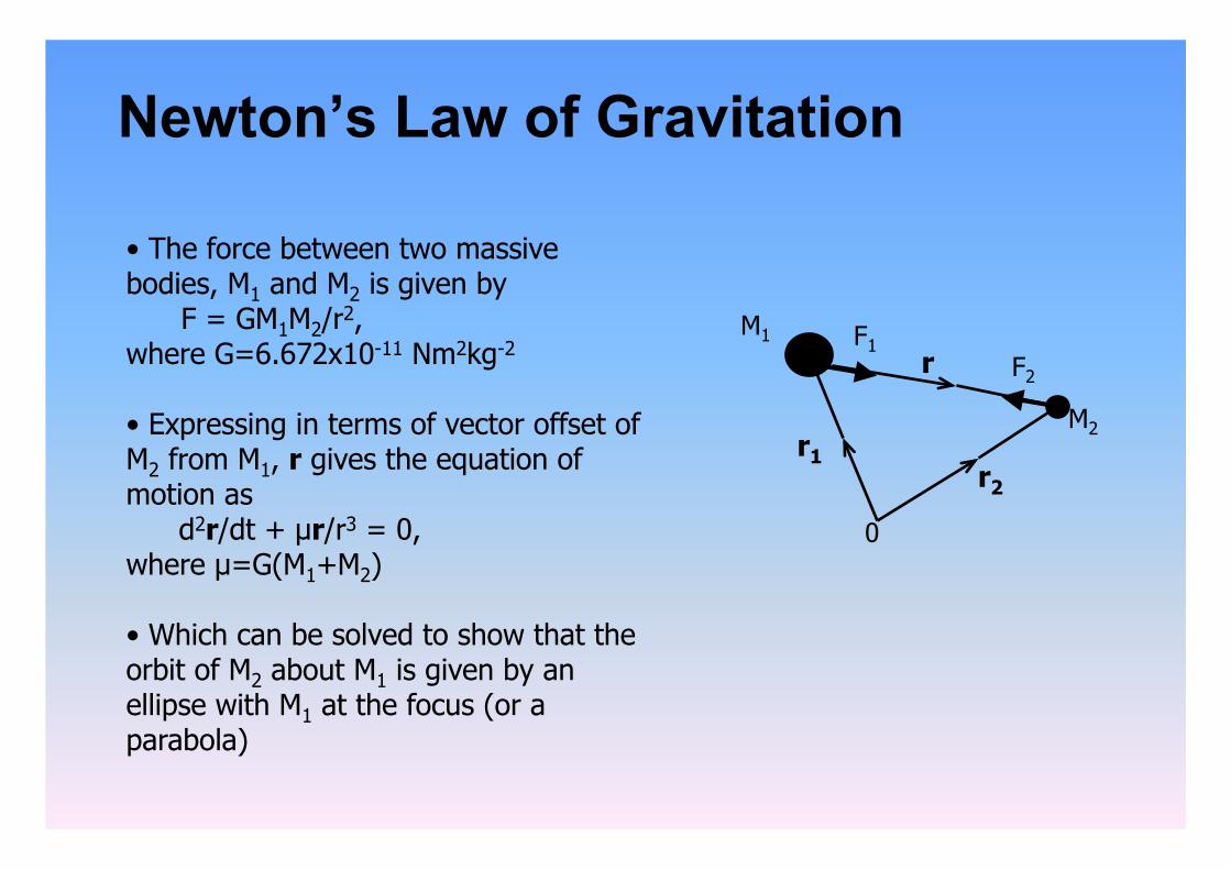
•  The force between two massive bodies, M1 and M2 is given by F = GM1M2/r2, where G=6.672x10-11 Nm2kg-2

•  Expressing in terms of vector offset of M2 from M1, r gives the equation of motion as

d2r/dt + µr/r3 = 0, where µ=G(M1+M2)

•  Which can be solved to show that the orbit of M2 about M1 is given by an ellipse with M1 at the focus (or a parabola)

M2

0

r1 r2

M1 r

F1 F2

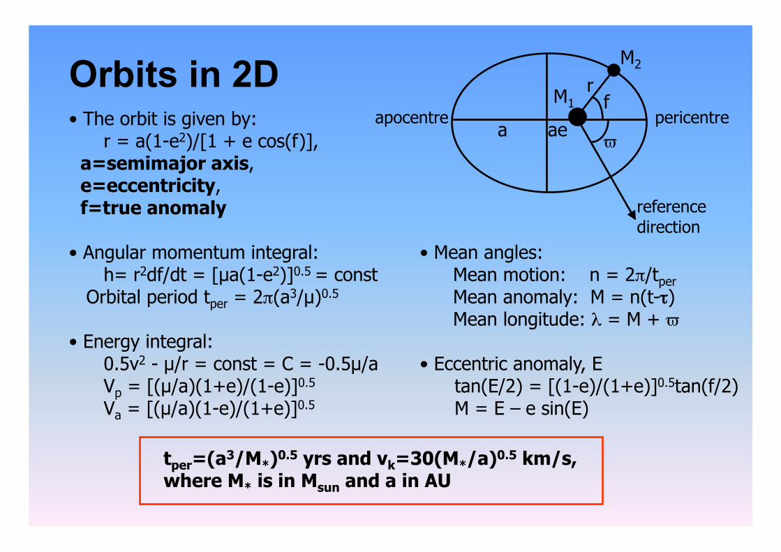
Orbits in 2D •  The orbit is given by: r = a(1-e2)/[1 + e cos(f)], a=semimajor axis, e=eccentricity, f=true anomaly

•  Angular momentum integral: h= r2df/dt = [µa(1-e2)]0.5 = const Orbital period tper = 2π(a3/µ)0.5

•  Energy integral: 0.5v2 - µ/r = const = C = -0.5µ/a Vp = [(µ/a)(1+e)/(1-e)]0.5

Va = [(µ/a)(1-e)/(1+e)]0.5

tper=(a3/M*)0.5 yrs and vk=30(M*/a)0.5 km/s, where M* is in Msun and a in AU

pericentre apocentre ae

r

a f M1

M2

ϖ

reference direction

•  Mean angles: Mean motion: n = 2π/tper Mean anomaly: M = n(t-τ) Mean longitude: λ = M + ϖ

•  Eccentric anomaly, E tan(E/2) = [(1-e)/(1+e)]0.5tan(f/2) M = E – e sin(E)

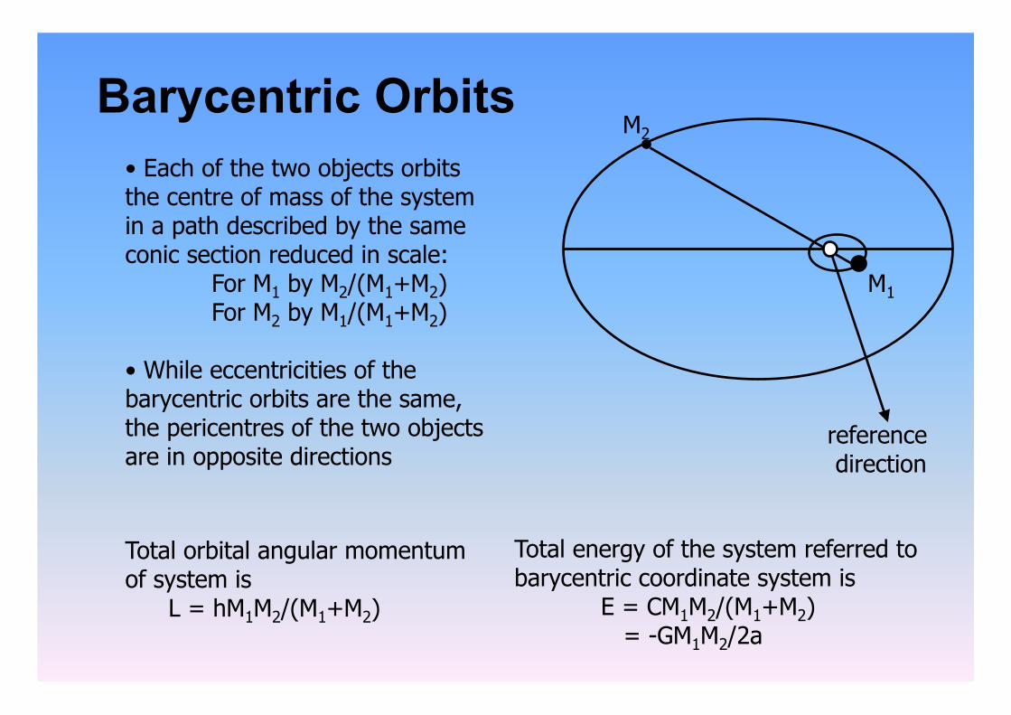
Barycentric Orbits •  Each of the two objects orbits the centre of mass of the system in a path described by the same conic section reduced in scale:

For M1 by M2/(M1+M2) For M2 by M1/(M1+M2)

•  While eccentricities of the barycentric orbits are the same, the pericentres of the two objects are in opposite directions

Total orbital angular momentum of system is

L = hM1M2/(M1+M2)

Total energy of the system referred to barycentric coordinate system is

E = CM1M2/(M1+M2) = -GM1M2/2a

reference direction

M1

M2

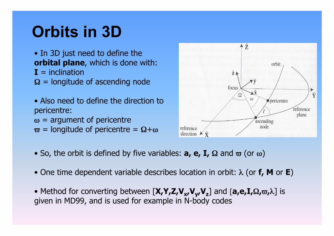
Orbits in 3D •  In 3D just need to define the orbital plane, which is done with: I = inclination Ω = longitude of ascending node

•  Also need to define the direction to pericentre: ω = argument of pericentre ϖ = longitude of pericentre = Ω+ω

•  So, the orbit is defined by five variables: a, e, I, Ω and ϖ (or ω)

•  One time dependent variable describes location in orbit: λ (or f, M or E)

•  Method for converting between [X,Y,Z,Vx,Vy,Vz] and [a,e,I,Ω,ϖ,λ] is given in MD99, and is used for example in N-body codes

Perturbed orbits

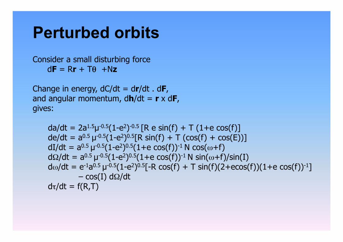
Consider a small disturbing force dF = Rr + Tθ +Nz

Change in energy, dC/dt = dr/dt . dF, and angular momentum, dh/dt = r x dF, gives:

da/dt = 2a1.5µ-0.5(1-e2)-0.5 [R e sin(f) + T (1+e cos(f)] de/dt = a0.5 µ-0.5(1-e2)0.5[R sin(f) + T (cos(f) + cos(E))]

dI/dt = a0.5 µ-0.5(1-e2)0.5(1+e cos(f))-1 N cos(ω+f) dΩ/dt = a0.5 µ-0.5(1-e2)0.5(1+e cos(f))-1 N sin(ω+f)/sin(I) dω/dt = e-1a0.5 µ-0.5(1-e2)0.5[-R cos(f) + T sin(f)(2+ecos(f))(1+e cos(f))-1] – cos(I) dΩ/dt dτ/dt = f(R,T)

Restricted 3 body problem

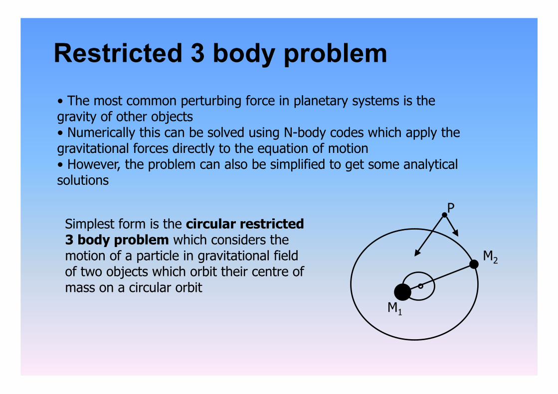
•  The most common perturbing force in planetary systems is the gravity of other objects •  Numerically this can be solved using N-body codes which apply the gravitational forces directly to the equation of motion •  However, the problem can also be simplified to get some analytical solutions

M1

Simplest form is the circular restricted 3 body problem which considers the motion of a particle in gravitational field of two objects which orbit their centre of mass on a circular orbit

M2

P

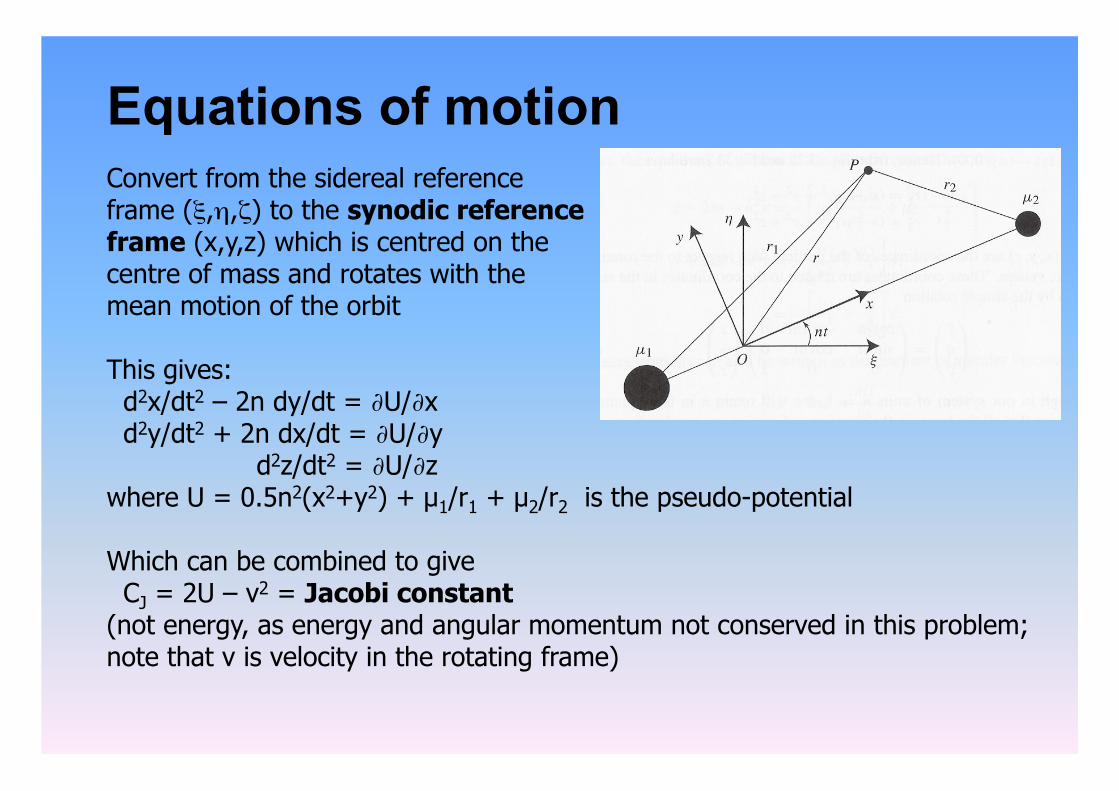
Equations of motion Convert from the sidereal reference frame (ξ,η,ζ) to the synodic reference frame (x,y,z) which is centred on the centre of mass and rotates with the mean motion of the orbit

This gives: d2x/dt2 – 2n dy/dt = ∂U/∂x d2y/dt2 + 2n dx/dt = ∂U/∂y d2z/dt2 = ∂U/∂z where U = 0.5n2(x2+y2) + µ1/r1 + µ2/r2 is the pseudo-potential

Which can be combined to give CJ = 2U – v2 = Jacobi constant (not energy, as energy and angular momentum not conserved in this problem; note that v is velocity in the rotating frame)

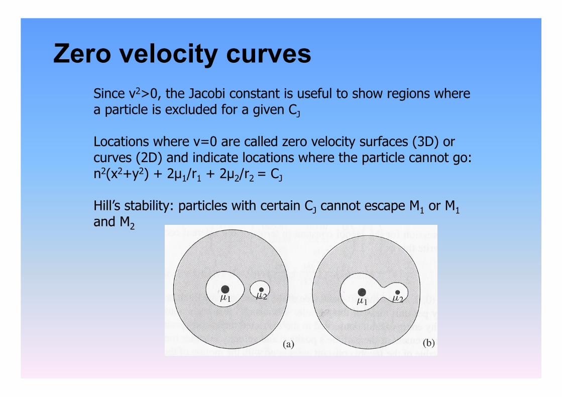
Zero velocity curves Since v2>0, the Jacobi constant is useful to show regions where a particle is excluded for a given CJ

Locations where v=0 are called zero velocity surfaces (3D) or curves (2D) and indicate locations where the particle cannot go: n2(x2+y2) + 2µ1/r1 + 2µ2/r2 = CJ

Hill’s stability: particles with certain CJ cannot escape M1 or M1 and M2

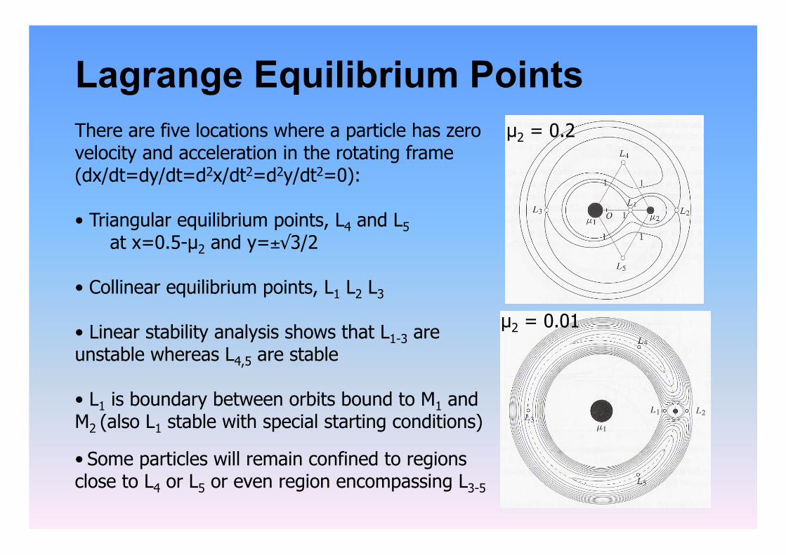
Lagrange Equilibrium Points There are five locations where a particle has zero velocity and acceleration in the rotating frame (dx/dt=dy/dt=d2x/dt2=d2y/dt2=0):

•  Triangular equilibrium points, L4 and L5 at x=0.5-µ2 and y=±√3/2

•  Collinear equilibrium points, L1 L2 L3

•  Linear stability analysis shows that L1-3 are unstable whereas L4,5 are stable

•  L1 is boundary between orbits bound to M1 and M2 (also L1 stable with special starting conditions)

•  Some particles will remain confined to regions close to L4 or L5 or even region encompassing L3-5

µ2 = 0.2

µ2 = 0.01

Tadpole/Horshoe Orbits

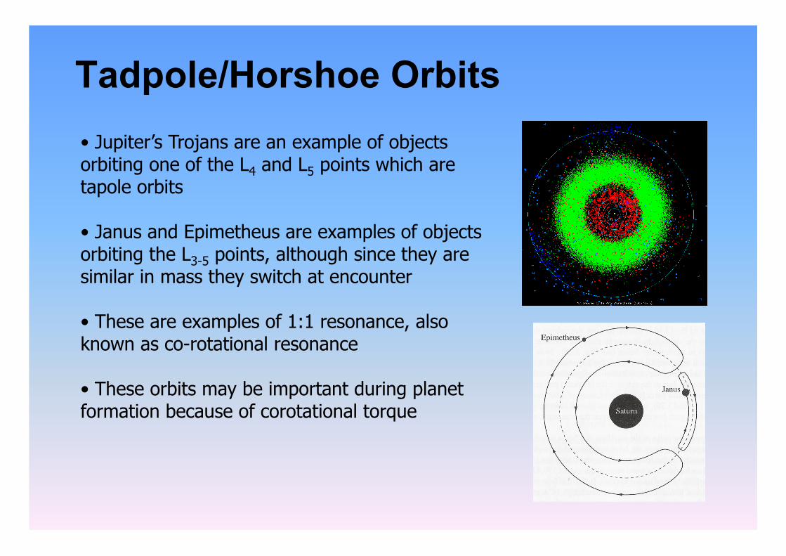
•  Jupiter’s Trojans are an example of objects orbiting one of the L4 and L5 points which are tapole orbits

•  Janus and Epimetheus are examples of objects orbiting the L3-5 points, although since they are similar in mass they switch at encounter

•  These are examples of 1:1 resonance, also known as co-rotational resonance

•  These orbits may be important during planet formation because of corotational torque

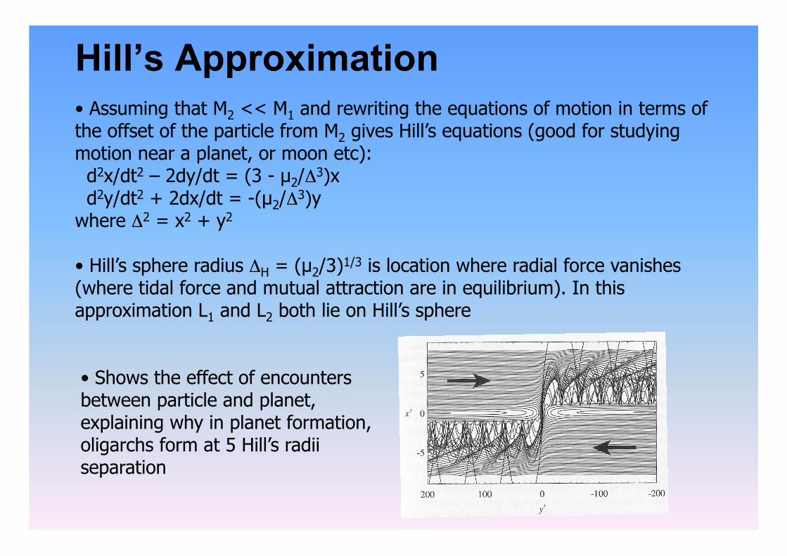
Hill’s Approximation •  Assuming that M2 << M1 and rewriting the equations of motion in terms of the offset of the particle from M2 gives Hill’s equations (good for studying motion near a planet, or moon etc): d2x/dt2 – 2dy/dt = (3 - µ2/Δ3)x d2y/dt2 + 2dx/dt = -(µ2/Δ3)y where Δ2 = x2 + y2

•  Hill’s sphere radius ΔH = (µ2/3)1/3 is location where radial force vanishes (where tidal force and mutual attraction are in equilibrium). In this approximation L1 and L2 both lie on Hill’s sphere

•  Shows the effect of encounters between particle and planet, explaining why in planet formation, oligarchs form at 5 Hill’s radii separation

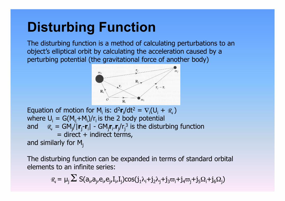
Disturbing Function The disturbing function is a method of calculating perturbations to an object’s elliptical orbit by calculating the acceleration caused by a perturbing potential (the gravitational force of another body)

Equation of motion for Mi is: d2ri/dt2 = ∇i(Ui + Ri ) where Ui = G(Mc+Mi)/ri is the 2 body potential and Ri = GMj/|rj-ri| - GMjri.rj/rj

3 is the disturbing function = direct + indirect terms, and similarly for Mj

The disturbing function can be expanded in terms of standard orbital elements to an infinite series:

Ri = µj Σ S(ai,aj,ei,ej,Ii,Ij)cos(j1λi+j2λj+j3ϖi+j4ϖj+j5Ωi+j6Ωj)

Different Types of Perturbations

Luckily for most problems we can take just one or two terms from the disturbing function using the averaging principle which states that most terms average to zero over a few orbital periods and so can be ignored by using the averaged disturbing function 〈R〉

Terms in the disturbing function can be divided into three types:

•  Secular Terms that don’t involve λi or λj which are slowly varying

•  Resonant Terms that involve angles φ = j1λi+j2λj+j3ϖi+j4ϖj+j5Ωi+j6Ωj where j1ni+j2nj = 0, since these too are slowly varying.

•  Short-period All other terms

Lagrange’s Planetary Equations •  The disturbing function can be used to determine the orbital variations of the perturbed body due to the perturbing potential

•  These are given in Lagrange’s planetary equations:

da/dt = (2/na)∂R/∂ε de/dt = -(1-e2)0.5(na2e)-1(1-(1-e2)0.5)∂R/∂ε - (1-e2)0.5(na2e)-1∂R/∂ϖ dΩ/dt = [na2(1-e2)sin(I)]-1∂R/∂I dϖ/dt = (1-e2)0.5(na2e)-1∂R/∂e + tan(I/2)(na2(1-e2))-1∂R/∂I dI/dt = -tan(I/2)(na2(1-e2)0.5)-1(∂R/∂ε + ∂R/∂ϖ) – (na2(1-e2)0.5sin(I))-1∂R/∂Ω dε/dt = -2(na)-1∂R/∂a + (1-e2)0.5(1-(1-e2)0.5)(na2e)-1∂R/∂e + tan(I/2)(na2(1-e2))-1 ∂R/∂I

where ε = λ - nt = ϖ - nτ

•  As with all equations, these can be simplified by taking terms to first order in e and I

Secular Perturbations •  To second order the secular terms of the disturbing function for the jth planet in a system with Npl planets are given by:

Rj = njaj2[0.5Ajj(ej

2-Ij2) + ΣNpl

i=1, i≠j Aijeiejcos(ϖi-ϖj) + BijIiIjcos(Ωi-Ωj)]

where Ajj = 0.25nj ΣNpli=1,i≠j (Mi/M*)αjiαjib1

3/2(αjj) Aji = -0.25nj(Mi/M*) αjiαjib2

3/2(αji) Bji = 0.25nj(Mi/M*) αjiαjib1

3/2(αji) αji and αji are functions of ai/aj and bs

3/2(αji) are Laplace coefficients

•  Converting to a system with zj = ej exp(iϖj) and yj = Ij exp(iΩj) and combining the planet variables into vectors z = [z1,z2,…,zNpl]T and for y gives for Lagrange’s planetary equations daj/dt = 0, dz/dt = iAz, dy/dt = iBy, where A,B are matrices of Aji,Bji

•  This can be solved to give: zj = ΣNpl

k=1 ejk exp(igk+iβk) and yj = ΣNplk=1 Ijk exp(ifkt+iγk)

where gk and fk are the eigenfrequencies of A and B and βk γk are the constants

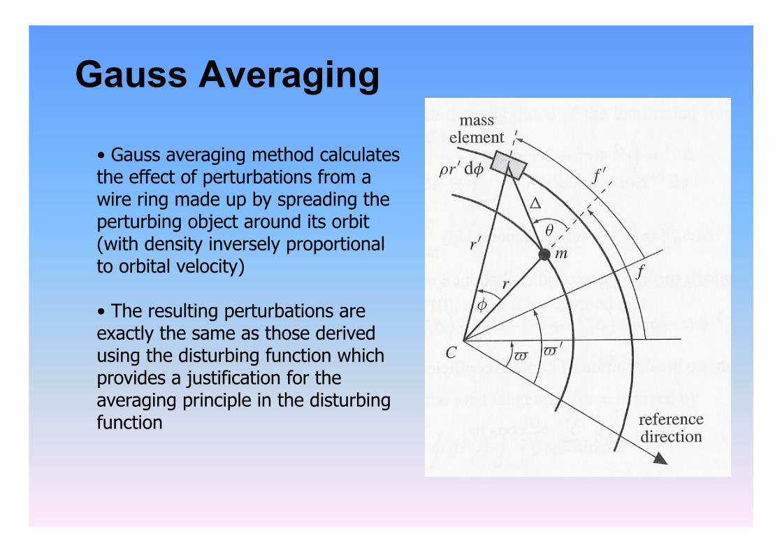
Gauss Averaging

•  Gauss averaging method calculates the effect of perturbations from a wire ring made up by spreading the perturbing object around its orbit (with density inversely proportional to orbital velocity)

•  The resulting perturbations are exactly the same as those derived using the disturbing function which provides a justification for the averaging principle in the disturbing function

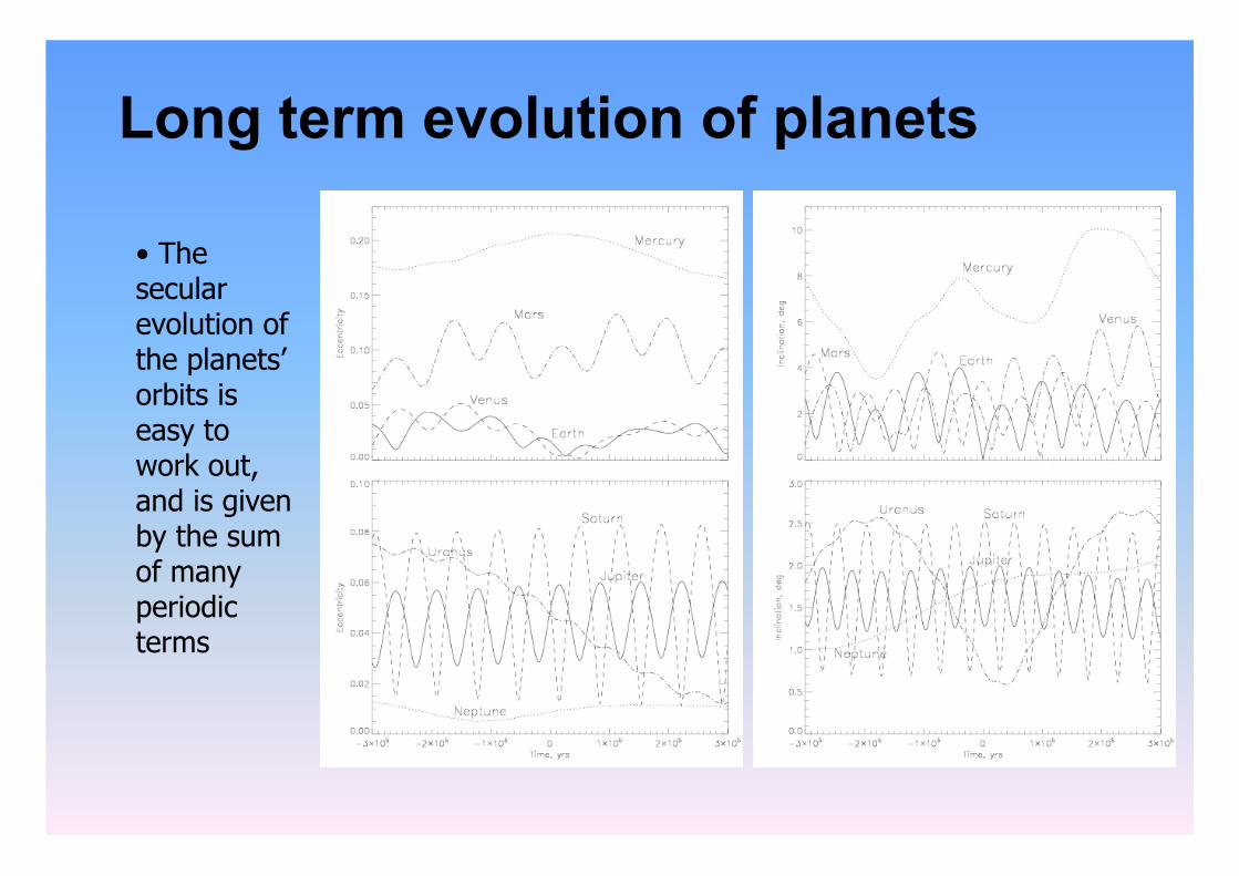
Long term evolution of planets

•  The secular evolution of the planets’ orbits is easy to work out, and is given by the sum of many periodic terms

Secular perturbations on particles •  The secular terms of the disturbing function for a particle in a system with Npl planets are given by:

R = na2[0.5A(e2-I2) + ΣNplj=1 Ajeejcos(ϖ-ϖj) + BjIIjcos(Ω-Ωj)]

where A = 0.25n ΣNplj=1 (Mj/M*)αjαjb1

3/2(αj) Aj = -0.25n(Mj/M*) αjαjb2

3/2(αj) Bj = 0.25n(Mj/M*) αjαjb1

3/2(αj) αj and αj are functions of a/aj and bs

3/2(αj) are Laplace coefficients

•  Which gives for Lagrange’s planetary equations: da/dt = 0 dz/dt = iAz + iΣNpl

j=1 Ajzj dy/dt = -iAy + iΣNpl

j=1 Bjyj

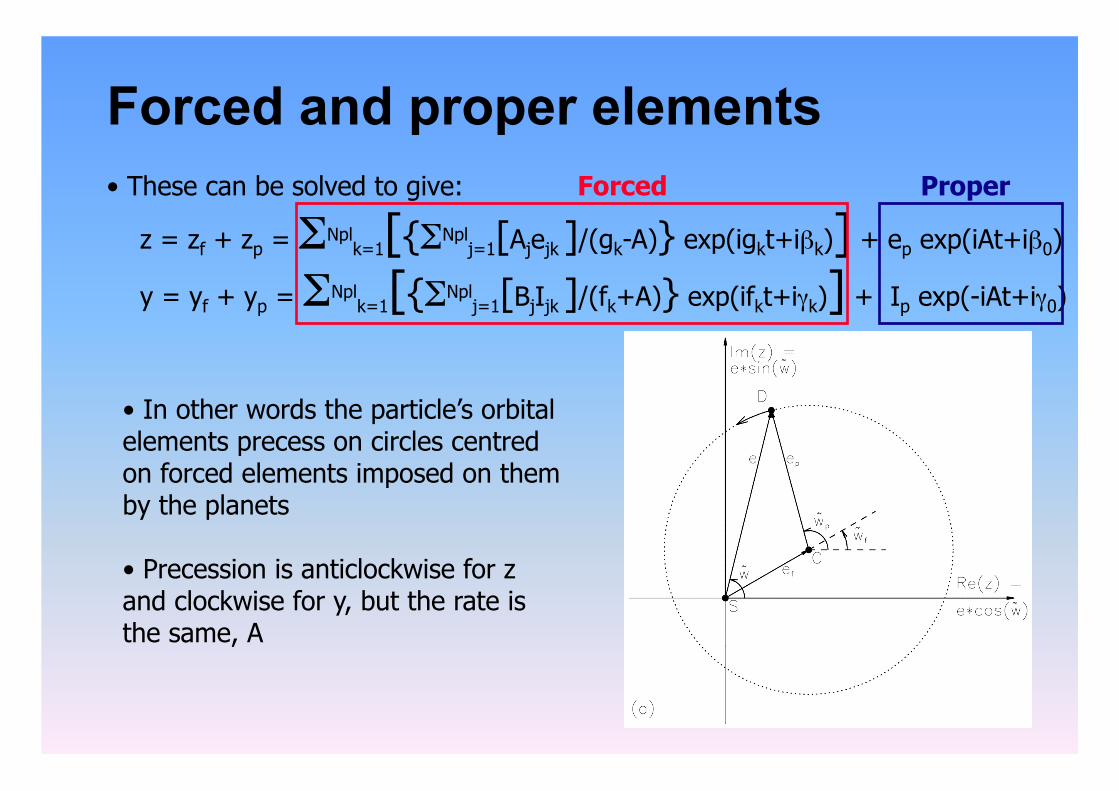
Forced and proper elements •  These can be solved to give:

z = zf + zp = ΣNplk=1[{ΣNpl

j=1[Ajejk ]/(gk-A)} exp(igkt+iβk)] + ep exp(iAt+iβ0)

y = yf + yp = ΣNplk=1[{ΣNpl

j=1[BjIjk ]/(fk+A)} exp(ifkt+iγk)] + Ip exp(-iAt+iγ0)

•  In other words the particle’s orbital elements precess on circles centred on forced elements imposed on them by the planets

•  Precession is anticlockwise for z and clockwise for y, but the rate is the same, A

Forced Proper

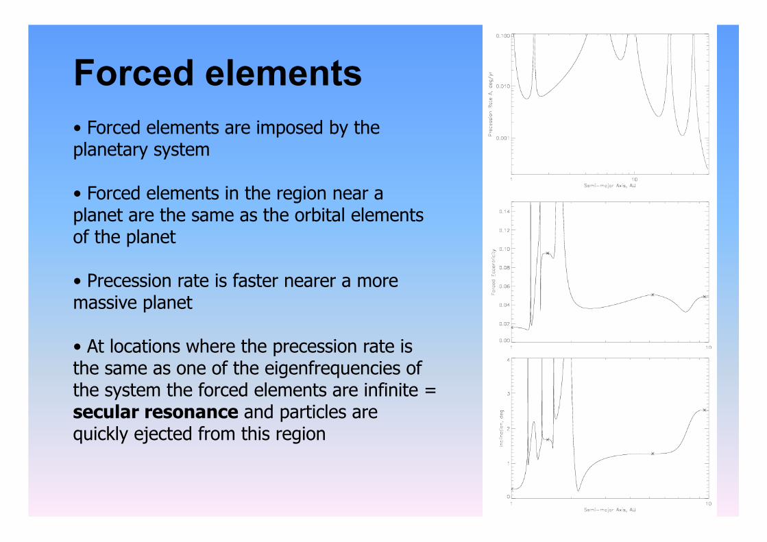
Forced elements •  Forced elements are imposed by the planetary system

•  Forced elements in the region near a planet are the same as the orbital elements of the planet

•  Precession rate is faster nearer a more massive planet

•  At locations where the precession rate is the same as one of the eigenfrequencies of the system the forced elements are infinite = secular resonance and particles are quickly ejected from this region

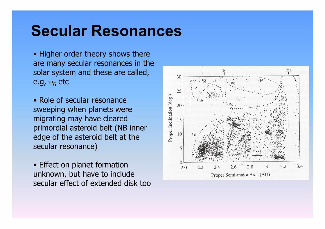
Secular Resonances •  Higher order theory shows there are many secular resonances in the solar system and these are called, e.g, υ6 etc

•  Role of secular resonance sweeping when planets were migrating may have cleared primordial asteroid belt (NB inner edge of the asteroid belt at the secular resonance)

•  Effect on planet formation unknown, but have to include secular effect of extended disk too

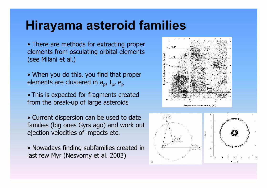
Hirayama asteroid families •  There are methods for extracting proper elements from osculating orbital elements (see Milani et al.)

•  When you do this, you find that proper elements are clustered in ap, Ip, ep

•  This is expected for fragments created from the break-up of large asteroids

•  Current dispersion can be used to date families (big ones Gyrs ago) and work out ejection velocities of impacts etc.

•  Nowadays finding subfamilies created in last few Myr (Nesvorny et al. 2003)

Resonant perturbations •  Resonances occur at specific locations where j1ni + j2nj ≈ 0, which means that the orbital periods are a ratio of two integers, from which we get that aj/ai = (|j1|/|j2|)2/3 = nominal resonance location

•  The terms in the disturbing function are given by those which satisfy that criterion, but there are infinite number of terms that nearly satisfy that condition

•  Generally it is the lowest order terms that dominate because of the strength of resonances:

Ri = µj Σ S(ai,aj,ei,ej,Ii,Ij)cos(j1λi+j2λj+j3ϖi+j4ϖj+j5Ωi+j6Ωj) S ≈ f(α)aj

-1ei|j4|ej

|j3|[sin(Ii/2)]|j6|[sin(Ij/2)]|j5| Σ6

i=1 ji = 0

which means that for a (p+q)λi-pλj-qϖi resonance, the strength is ∝eq in

other words the q=1 resonances (first order resonances) are strongest and so the 3:2 term is more important than the 6:4 term or 301:200

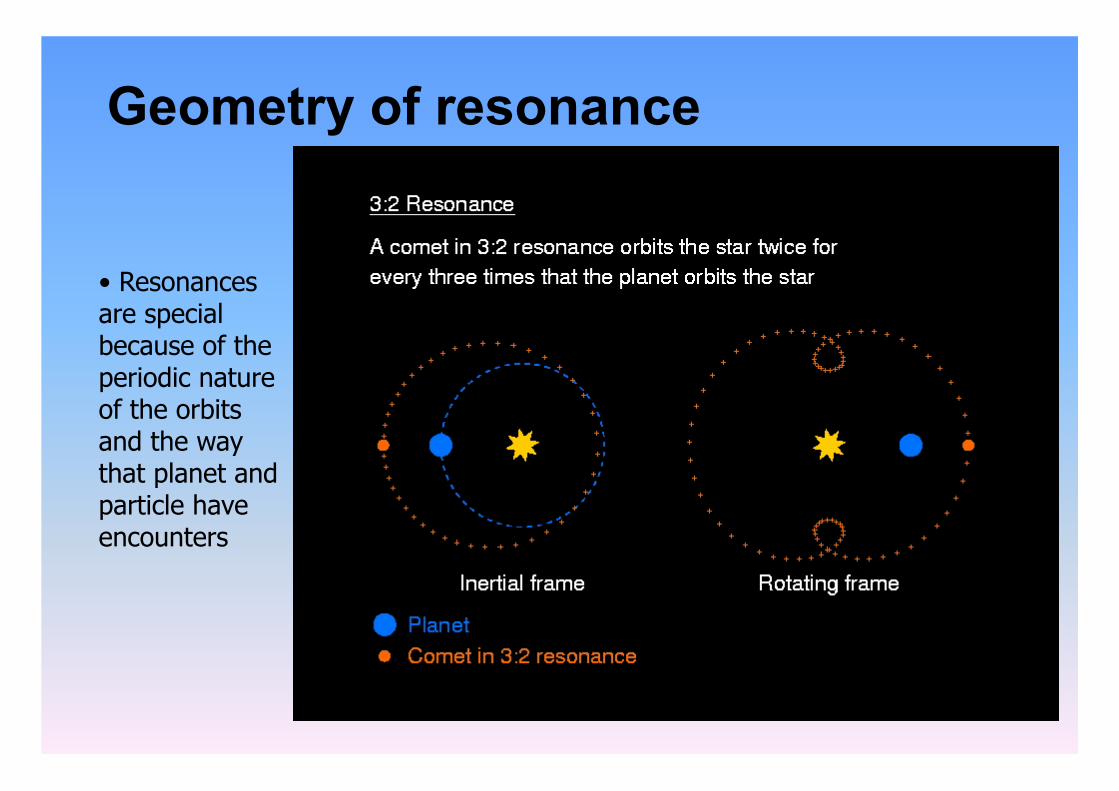
Geometry of resonance

•  Resonances are special because of the periodic nature of the orbits and the way that planet and particle have encounters

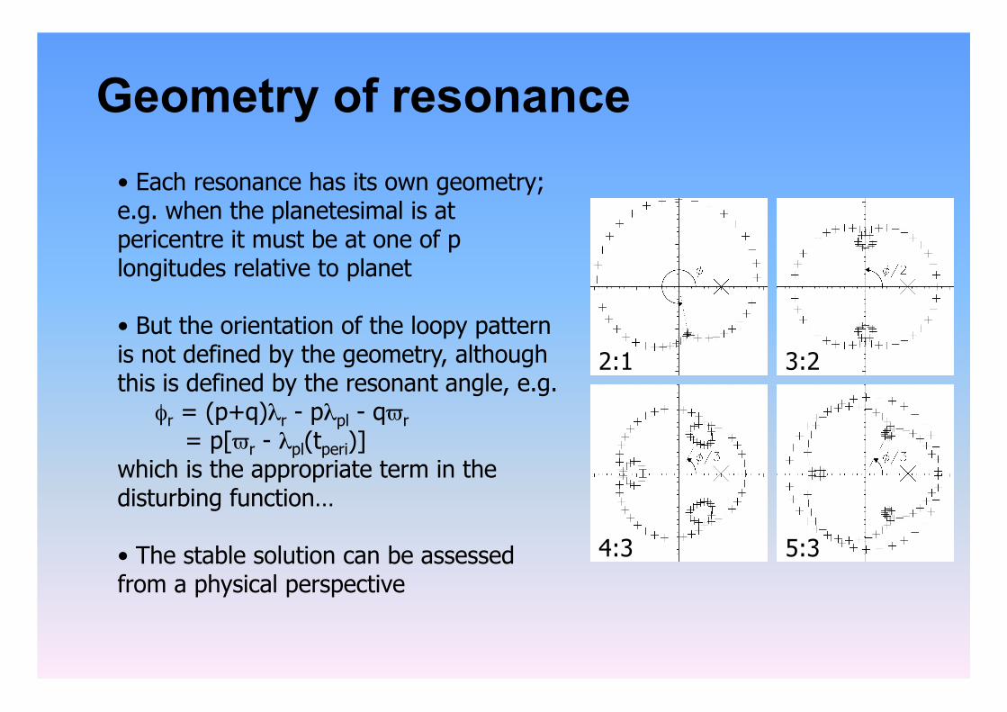
Geometry of resonance •  Each resonance has its own geometry; e.g. when the planetesimal is at pericentre it must be at one of p longitudes relative to planet

•  But the orientation of the loopy pattern is not defined by the geometry, although this is defined by the resonant angle, e.g. φr = (p+q)λr - pλpl - qϖr = p[ϖr - λpl(tperi)] which is the appropriate term in the disturbing function…

•  The stable solution can be assessed from a physical perspective

2:1

5:3 4:3

3:2

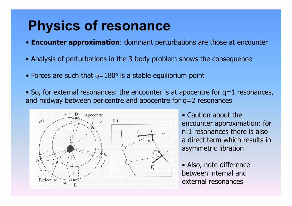
Physics of resonance •  Encounter approximation: dominant perturbations are those at encounter

•  Analysis of perturbations in the 3-body problem shows the consequence

•  Forces are such that φ=180o is a stable equilibrium point

•  So, for external resonances: the encounter is at apocentre for q=1 resonances, and midway between pericentre and apocentre for q=2 resonances

•  Caution about the encounter approximation: for n:1 resonances there is also a direct term which results in asymmetric libration

•  Also, note difference between internal and external resonances

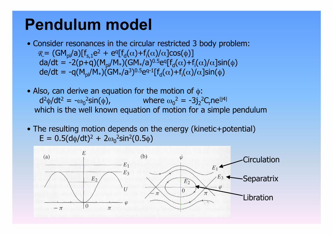
Pendulum model •  Consider resonances in the circular restricted 3 body problem: R = (GMpl/a)[fs,1e2 + eq[fd(α)+fi(α)/α]cos(φ)] da/dt = -2(p+q)(Mpl/M*)(GM*/a)0.5eq[fd(α)+fi(α)/α]sin(φ) de/dt = -q(Mpl/M*)(GM*/a3)0.5eq-1[fd(α)+fi(α)/α]sin(φ)

•  Also, can derive an equation for the motion of φ: d2φ/dt2 = -ω0

2sin(φ), where ω02 = -3j22Crne|j4|

which is the well known equation of motion for a simple pendulum

•  The resulting motion depends on the energy (kinetic+potential) E = 0.5(dφ/dt)2 + 2ω0

2sin2(0.5φ)

Circulation

Separatrix

Libration

Libration/Circulation

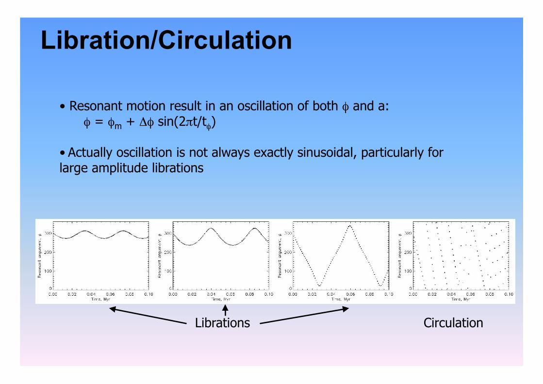
•  Resonant motion result in an oscillation of both φ and a: φ = φm + Δφ sin(2πt/tφ)

•  Actually oscillation is not always exactly sinusoidal, particularly for large amplitude librations

Librations Circulation

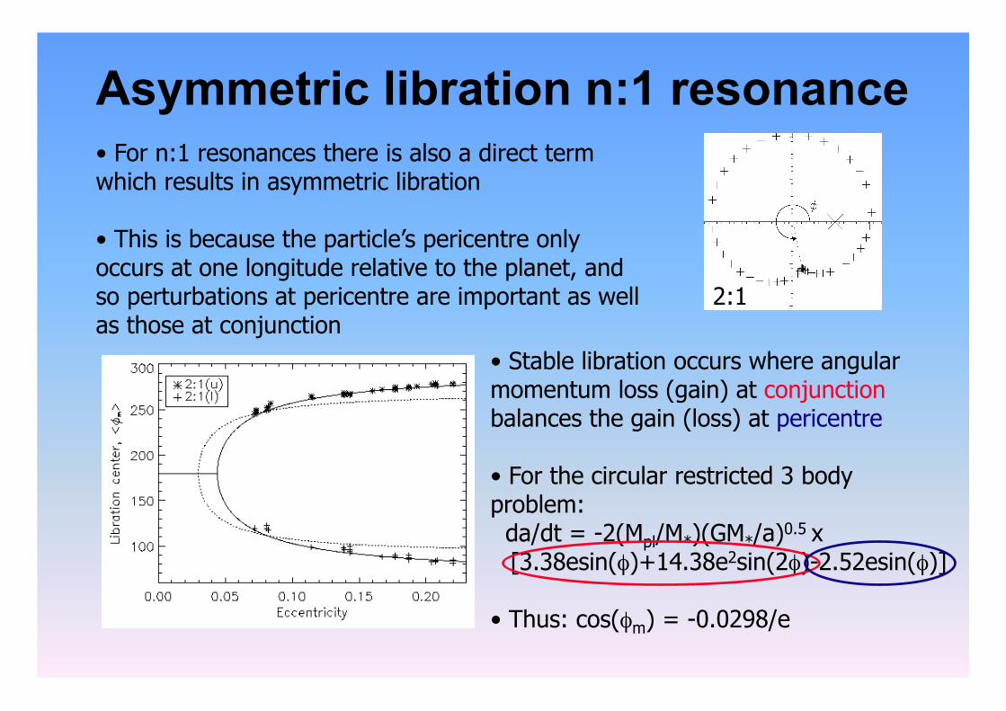
Asymmetric libration n:1 resonance

•  Stable libration occurs where angular momentum loss (gain) at conjunction balances the gain (loss) at pericentre

•  For the circular restricted 3 body problem: da/dt = -2(Mpl/M*)(GM*/a)0.5 x

[3.38esin(φ)+14.38e2sin(2φ)-2.52esin(φ)]

•  Thus: cos(φm) = -0.0298/e

•  For n:1 resonances there is also a direct term which results in asymmetric libration

•  This is because the particle’s pericentre only occurs at one longitude relative to the planet, and so perturbations at pericentre are important as well as those at conjunction

2:1

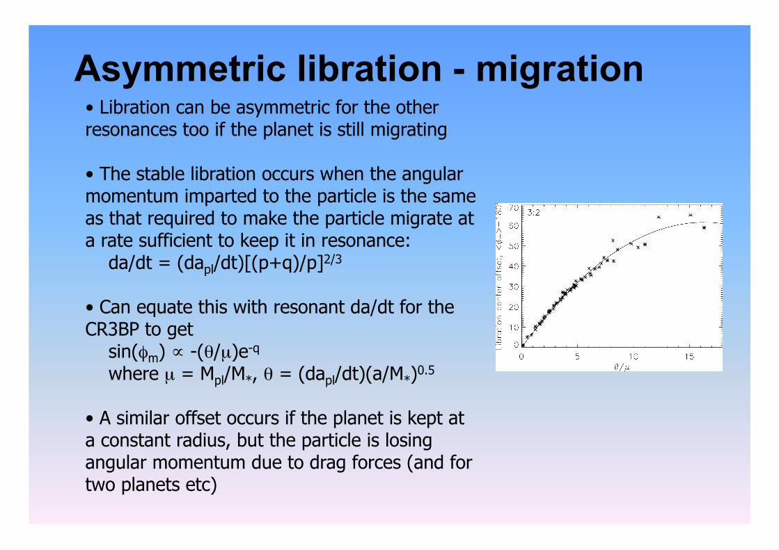
Asymmetric libration - migration •  Libration can be asymmetric for the other resonances too if the planet is still migrating

•  The stable libration occurs when the angular momentum imparted to the particle is the same as that required to make the particle migrate at a rate sufficient to keep it in resonance: da/dt = (dapl/dt)[(p+q)/p]2/3

•  Can equate this with resonant da/dt for the CR3BP to get sin(φm) ∝ -(θ/µ)e-q where µ = Mpl/M*, θ = (dapl/dt)(a/M*)0.5

•  A similar offset occurs if the planet is kept at a constant radius, but the particle is losing angular momentum due to drag forces (and for two planets etc)

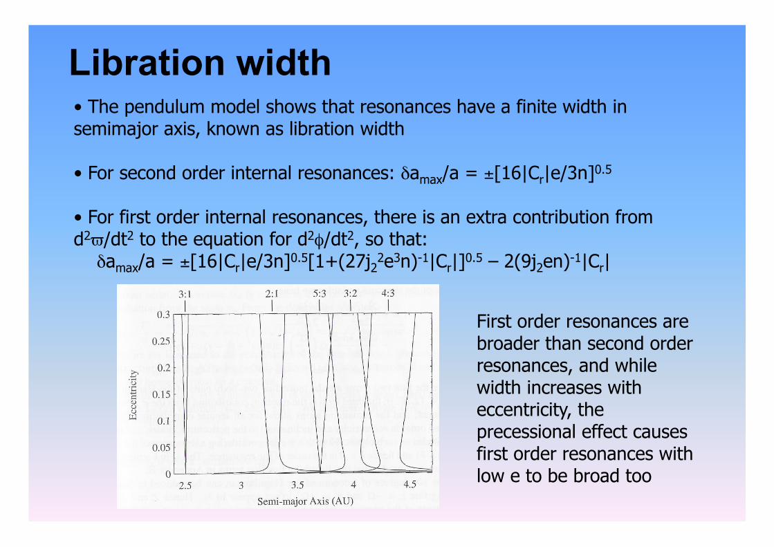
Libration width •  The pendulum model shows that resonances have a finite width in semimajor axis, known as libration width

•  For second order internal resonances: δamax/a = ±[16|Cr|e/3n]0.5

•  For first order internal resonances, there is an extra contribution from d2ϖ/dt2 to the equation for d2φ/dt2, so that: δamax/a = ±[16|Cr|e/3n]0.5[1+(27j22e3n)-1|Cr|]0.5 – 2(9j2en)-1|Cr|

First order resonances are broader than second order resonances, and while width increases with eccentricity, the precessional effect causes first order resonances with low e to be broad too

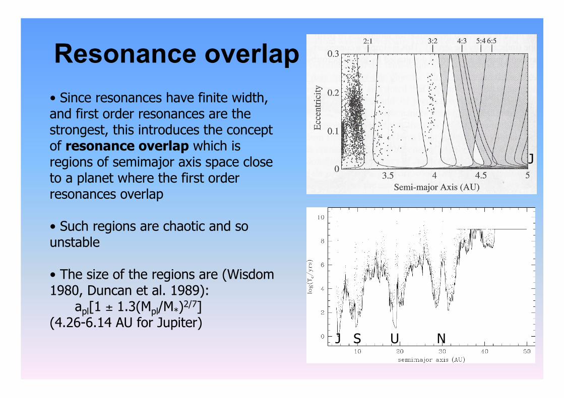
Resonance overlap •  Since resonances have finite width, and first order resonances are the strongest, this introduces the concept of resonance overlap which is regions of semimajor axis space close to a planet where the first order resonances overlap

•  Such regions are chaotic and so unstable

•  The size of the regions are (Wisdom 1980, Duncan et al. 1989): apl[1 ± 1.3(Mpl/M*)2/7] (4.26-6.14 AU for Jupiter)

J S U N

J

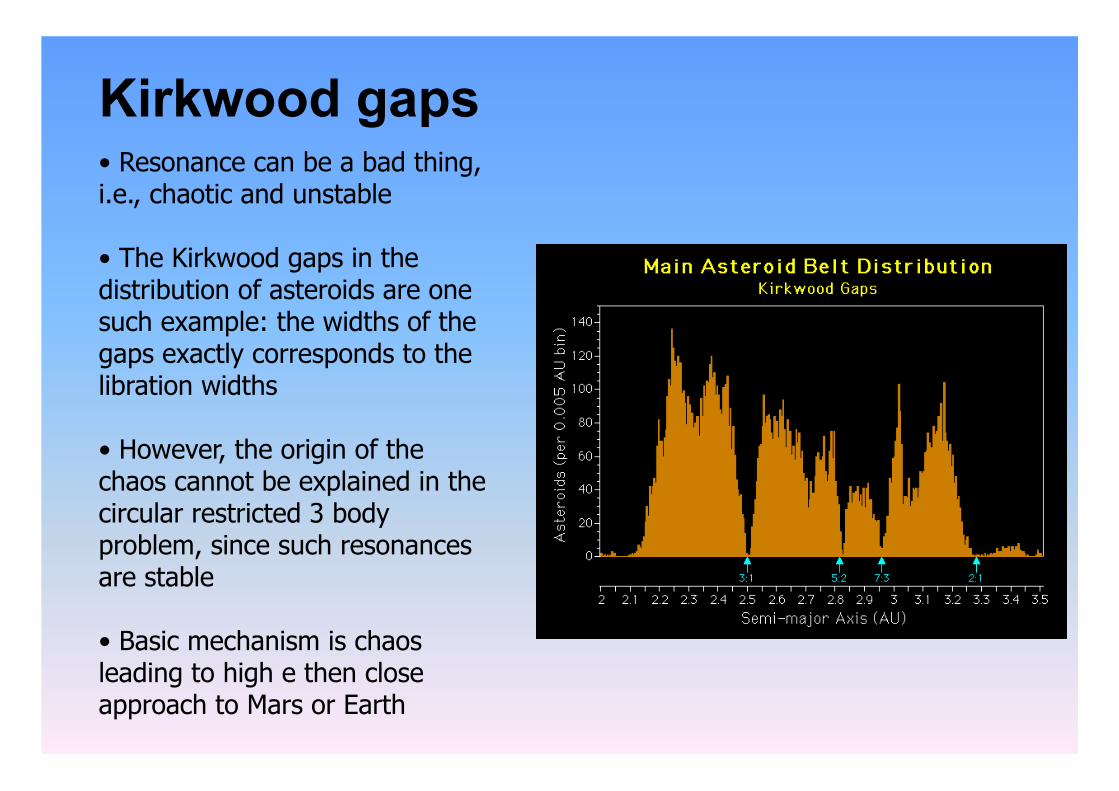
Kirkwood gaps •  Resonance can be a bad thing, i.e., chaotic and unstable

•  The Kirkwood gaps in the distribution of asteroids are one such example: the widths of the gaps exactly corresponds to the libration widths

•  However, the origin of the chaos cannot be explained in the circular restricted 3 body problem, since such resonances are stable

•  Basic mechanism is chaos leading to high e then close approach to Mars or Earth

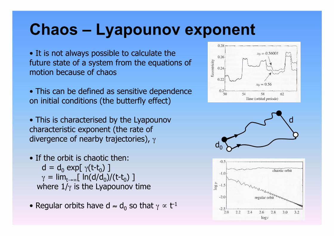
Chaos – Lyapounov exponent •  It is not always possible to calculate the future state of a system from the equations of motion because of chaos

•  This can be defined as sensitive dependence on initial conditions (the butterfly effect)

•  This is characterised by the Lyapounov characteristic exponent (the rate of divergence of nearby trajectories), γ

•  If the orbit is chaotic then: d = d0 exp[ γ(t-t0) ] γ = limt→∞[ ln(d/d0)/(t-t0) ] where 1/γ is the Lyapounov time

•  Regular orbits have d ≈ d0 so that γ ∝ t-1

d0

d

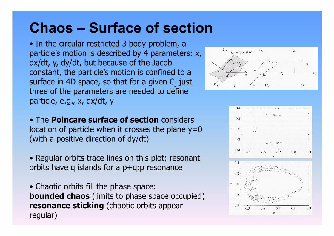
Chaos – Surface of section •  In the circular restricted 3 body problem, a particle’s motion is described by 4 parameters: x, dx/dt, y, dy/dt, but because of the Jacobi constant, the particle’s motion is confined to a surface in 4D space, so that for a given CJ just three of the parameters are needed to define particle, e.g., x, dx/dt, y

•  The Poincare surface of section considers location of particle when it crosses the plane y=0 (with a positive direction of dy/dt)

•  Regular orbits trace lines on this plot; resonant orbits have q islands for a p+q:p resonance

•  Chaotic orbits fill the phase space: bounded chaos (limits to phase space occupied) resonance sticking (chaotic orbits appear regular)

Fig. 9.3 from MD99

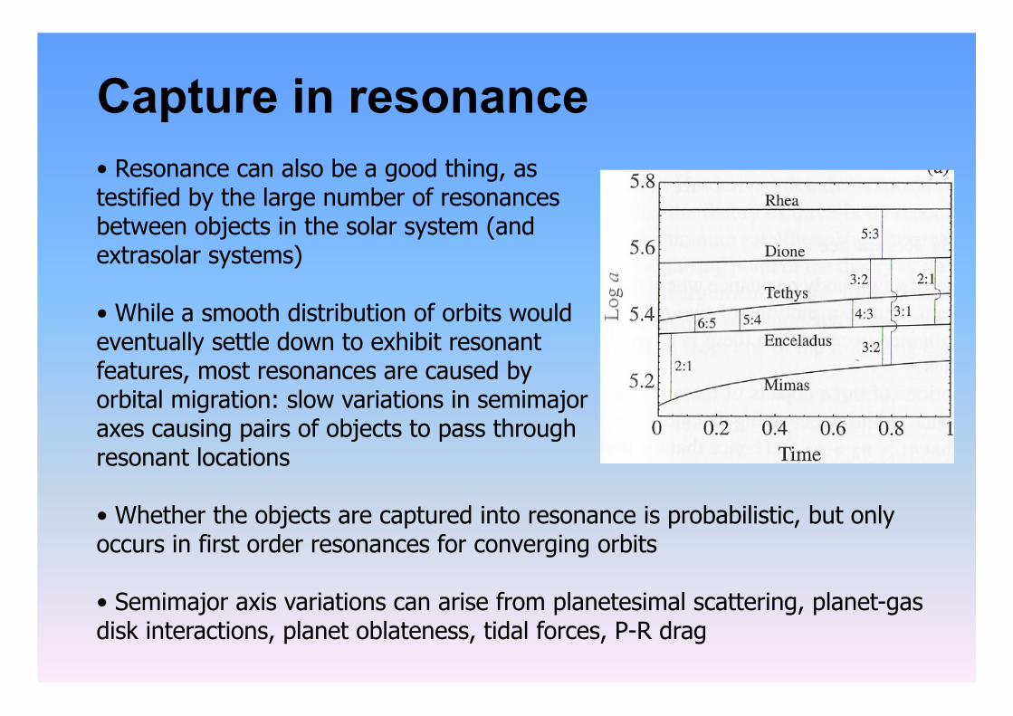
Capture in resonance •  Resonance can also be a good thing, as testified by the large number of resonances between objects in the solar system (and extrasolar systems)

•  While a smooth distribution of orbits would eventually settle down to exhibit resonant features, most resonances are caused by orbital migration: slow variations in semimajor axes causing pairs of objects to pass through resonant locations

•  Whether the objects are captured into resonance is probabilistic, but only occurs in first order resonances for converging orbits

•  Semimajor axis variations can arise from planetesimal scattering, planet-gas disk interactions, planet oblateness, tidal forces, P-R drag

Adiabatic Invariance

•  Resonance capture requires adiabiticity (Henrard 1982):

•  The libration period must be shorter than the time it takes for the resonance to cross the libration width dapl/dt << Δa/tφ

•  While it is possible to work out Δa and tφ for the CR3BP, this condition does not necessarily imply that capture will occur, for which more detailed studies are required (Friedland 2001; Wyatt 2003; Quillen et al. 2006)

•  Different approaches: numerical, or analytical – both are required

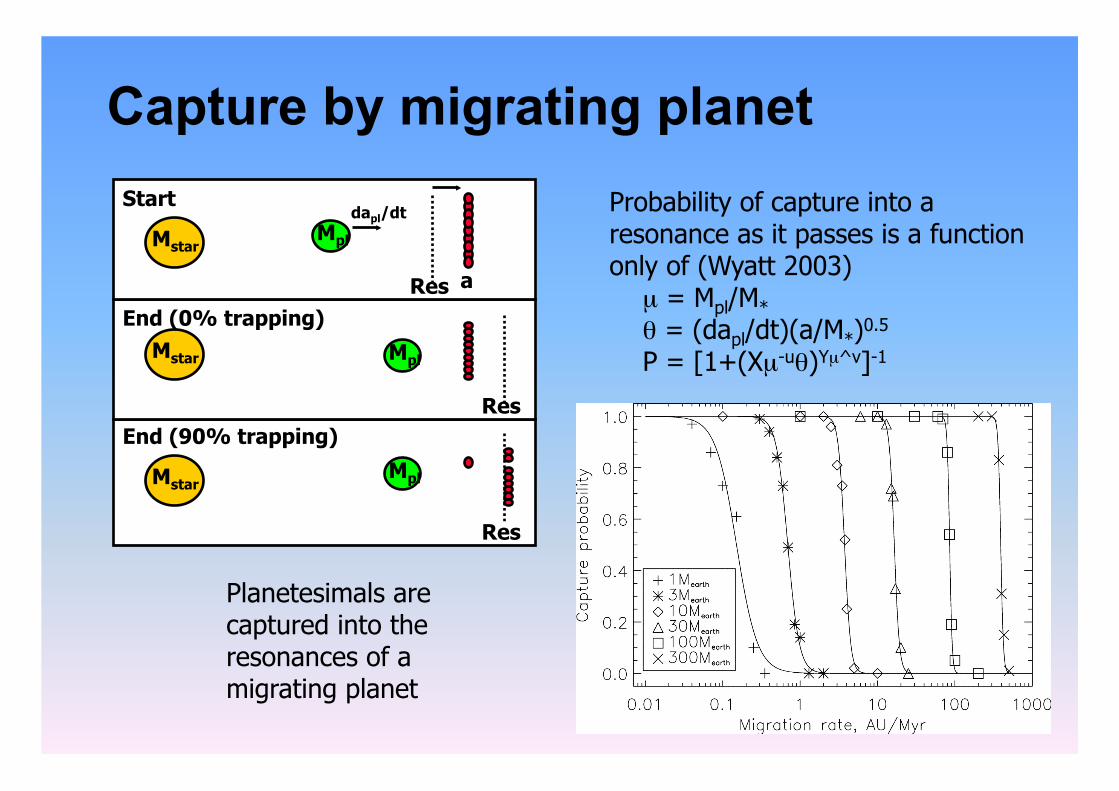
Capture by migrating planet Probability of capture into a resonance as it passes is a function only of (Wyatt 2003) µ = Mpl/M* θ = (dapl/dt)(a/M*)0.5

P = [1+(Xµ-uθ)Yµ^v]-1

Mpl

Res

Mpl

Res

Mpl

Res

Mstar

Mstar

Mstar

dapl/dt Start

End (0% trapping)

End (90% trapping)

a

Planetesimals are captured into the resonances of a migrating planet

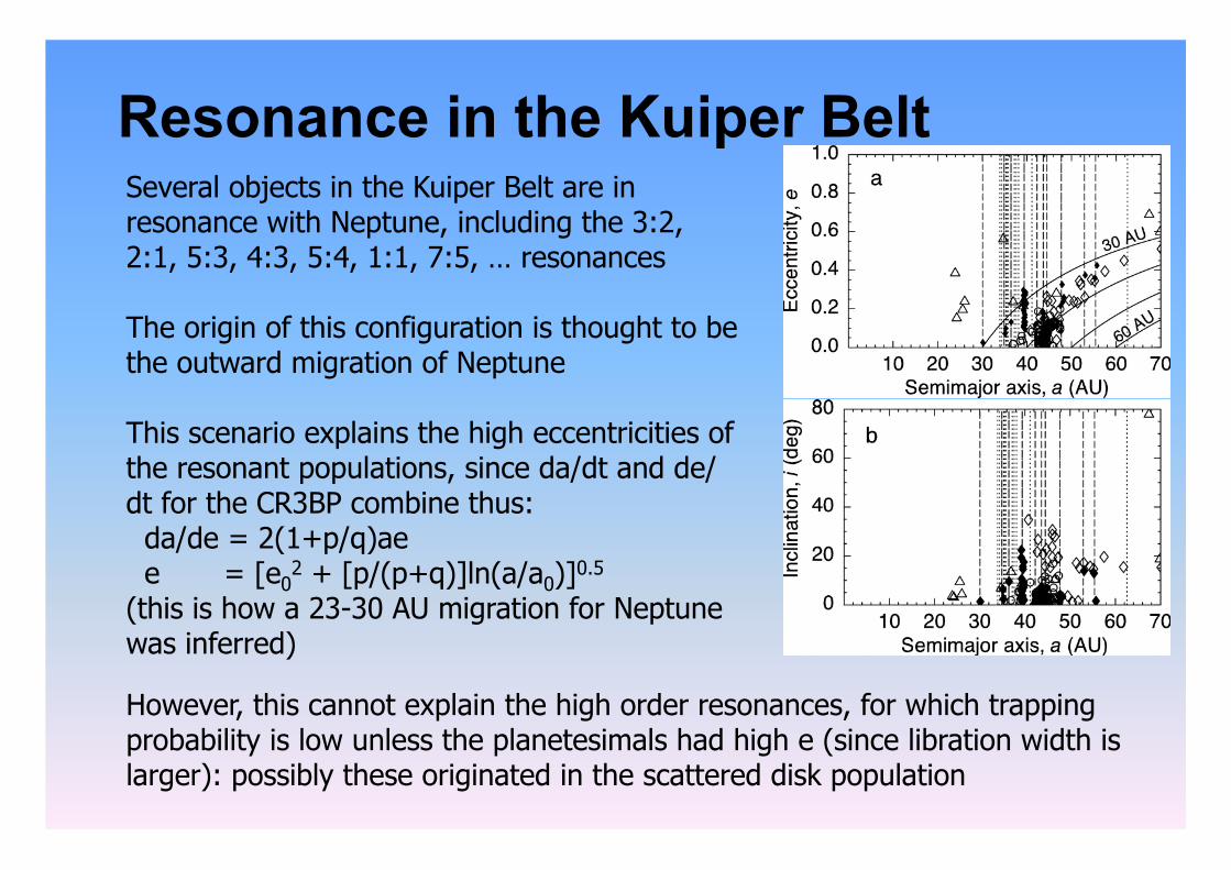
Several objects in the Kuiper Belt are in resonance with Neptune, including the 3:2, 2:1, 5:3, 4:3, 5:4, 1:1, 7:5, … resonances

The origin of this configuration is thought to be the outward migration of Neptune

This scenario explains the high eccentricities of the resonant populations, since da/dt and de/dt for the CR3BP combine thus: da/de = 2(1+p/q)ae e = [e0

2 + [p/(p+q)]ln(a/a0)]0.5 (this is how a 23-30 AU migration for Neptune was inferred)

Resonance in the Kuiper Belt

However, this cannot explain the high order resonances, for which trapping probability is low unless the planetesimals had high e (since libration width is larger): possibly these originated in the scattered disk population

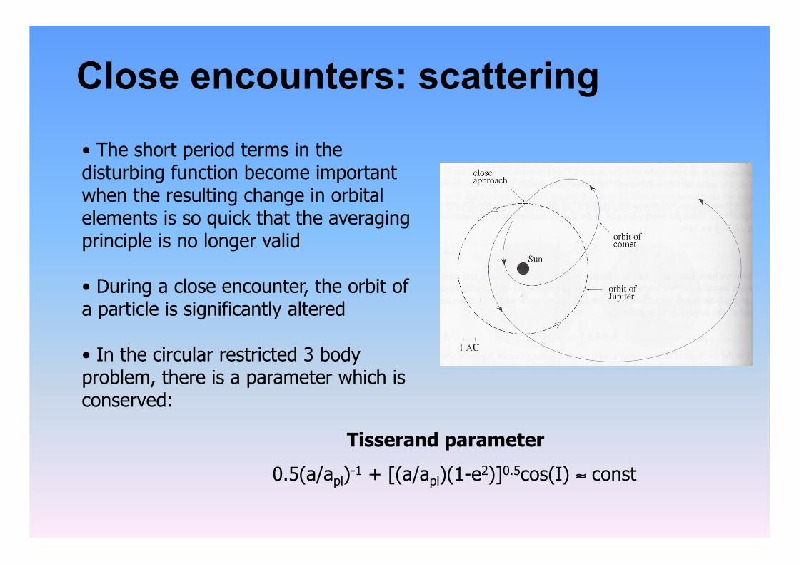
Close encounters: scattering

•  The short period terms in the disturbing function become important when the resulting change in orbital elements is so quick that the averaging principle is no longer valid

•  During a close encounter, the orbit of a particle is significantly altered

•  In the circular restricted 3 body problem, there is a parameter which is conserved:

Tisserand parameter

0.5(a/apl)-1 + [(a/apl)(1-e2)]0.5cos(I) ≈ const

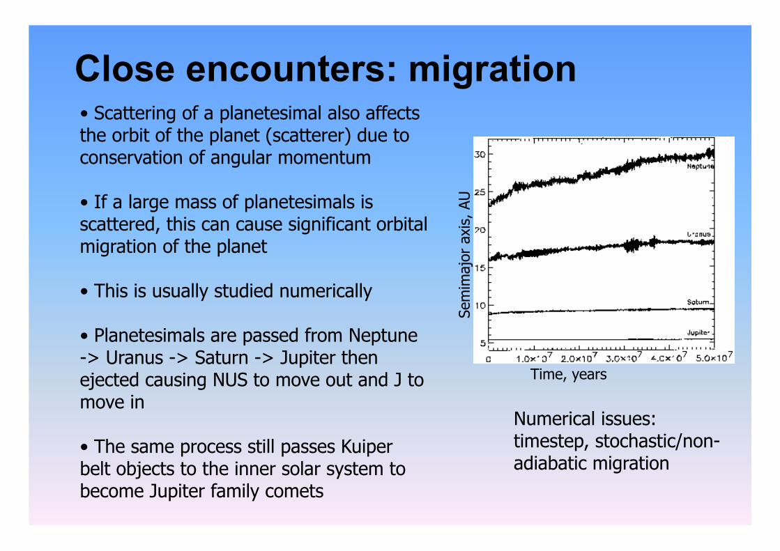
Close encounters: migration •  Scattering of a planetesimal also affects the orbit of the planet (scatterer) due to conservation of angular momentum

•  If a large mass of planetesimals is scattered, this can cause significant orbital migration of the planet

•  This is usually studied numerically

•  Planetesimals are passed from Neptune -> Uranus -> Saturn -> Jupiter then ejected causing NUS to move out and J to move in

•  The same process still passes Kuiper belt objects to the inner solar system to become Jupiter family comets

Time, years

Sem

imaj

or a

xis,

AU

Numerical issues: timestep, stochastic/non-adiabatic migration

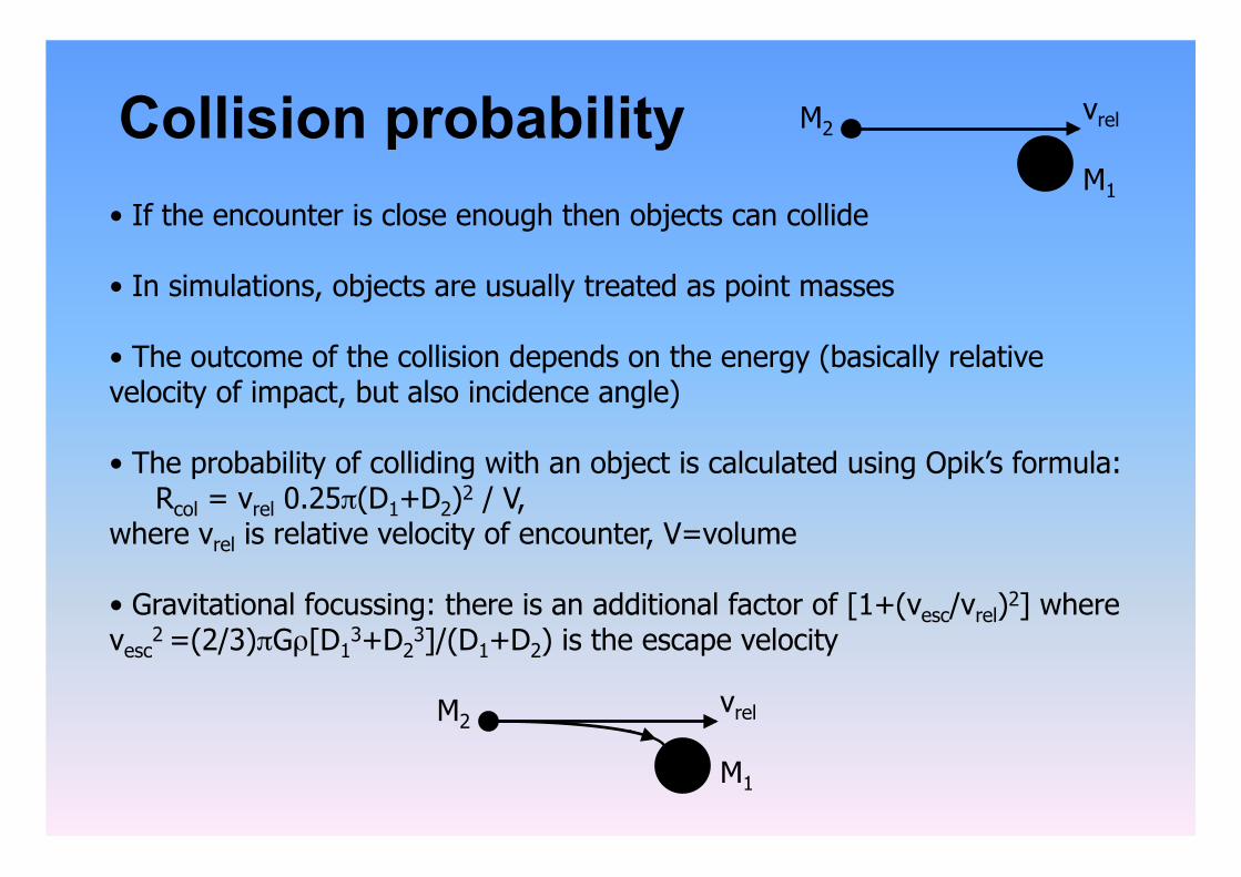
Collision probability •  If the encounter is close enough then objects can collide

•  In simulations, objects are usually treated as point masses

•  The outcome of the collision depends on the energy (basically relative velocity of impact, but also incidence angle)

•  The probability of colliding with an object is calculated using Opik’s formula: Rcol = vrel 0.25π(D1+D2)2 / V, where vrel is relative velocity of encounter, V=volume

•  Gravitational focussing: there is an additional factor of [1+(vesc/vrel)2] where vesc

2 =(2/3)πGρ[D1

3+D23]/(D1+D2) is the escape velocity

M1

M2 vrel

M1

M2 vrel

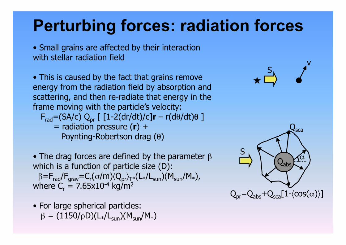
Perturbing forces: radiation forces •  Small grains are affected by their interaction with stellar radiation field

•  This is caused by the fact that grains remove energy from the radiation field by absorption and scattering, and then re-radiate that energy in the frame moving with the particle’s velocity: Frad=(SA/c) Qpr [ [1-2(dr/dt)/c]r – r(dθ/dt)θ ] = radiation pressure (r) + Poynting-Robertson drag (θ)

•  The drag forces are defined by the parameter β which is a function of particle size (D): β=Frad/Fgrav=Cr(σ/m)〈Qpr〉T*(L*/Lsun)(Msun/M*), where Cr = 7.65x10-4 kg/m2

•  For large spherical particles: β = (1150/ρD)(L*/Lsun)(Msun/M*)

Qabs

S

S

v

Qsca

Qpr=Qabs+Qsca[1-〈cos(α)〉]

α

Radiation pressure

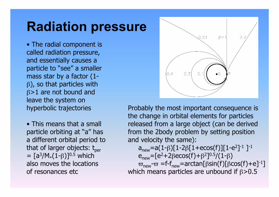
Probably the most important consequence is the change in orbital elements for particles released from a large object (can be derived from the 2body problem by setting position and velocity the same): anew=a(1-β)[1-2β[1+ecos(f)][1-e2]-1 ]-1 enew=[e2+2βecos(f)+β2]0.5/(1-β) ϖnew-ϖ =f-fnew=arctan[βsin(f)[βcos(f)+e]-1] which means particles are unbound if β>0.5

•  The radial component is called radiation pressure, and essentially causes a particle to “see” a smaller mass star by a factor (1-β), so that particles with β>1 are not bound and leave the system on hyperbolic trajectories

•  This means that a small particle orbiting at “a” has a different orbital period to that of larger objects: tper = [a3/M*(1-β)]0.5 which also moves the locations of resonances etc

Poynting-Robertson drag •  Poynting-Robertson drag causes dust grains to spiral into the star while at the same time circularising their orbits (dIpr/dt=dΩpr/dt=0): dapr/dt = -(α/a) (2+3e2)(1-e2)-1.5 ≈ -2α/a depr/dt = -2.5 (α/a2) e(1-e2)-0.5 ≈ -2.5eα/a2 where α = 6.24x10-4(M*/Msun)β AU2/yr

•  So time for a particle to migrate in from a1 to a2 is tpr = 400(Msun/M*)[a1

2 – a22]/β years

•  Also, considering continuity equation, the number density n(a) ∝ a which translates into constant surface density

•  On their way in particles can become trapped in resonance with interior planets, or be scattered, or accreted, or pass through secular resonances…

•  Large particles move slower, and so suffer no migration before being destroyed in a collision with another large particle

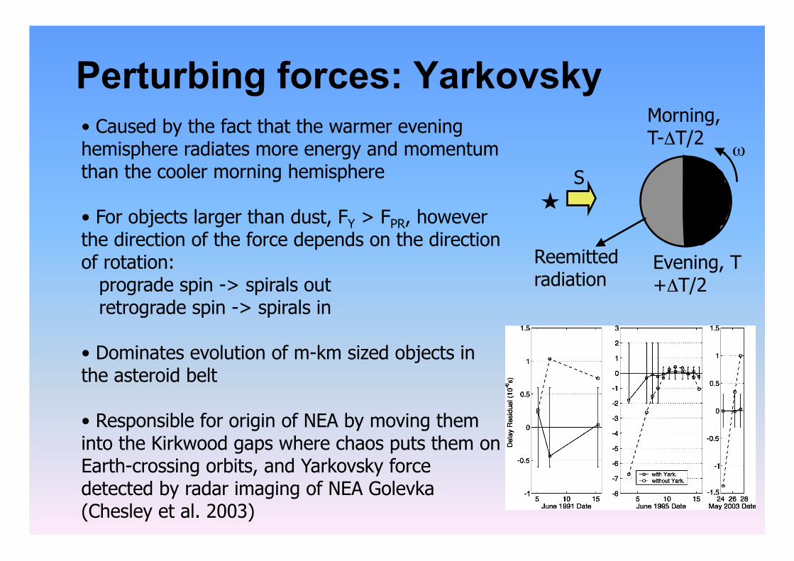
Perturbing forces: Yarkovsky •  Caused by the fact that the warmer evening hemisphere radiates more energy and momentum than the cooler morning hemisphere

•  For objects larger than dust, FY > FPR, however the direction of the force depends on the direction of rotation: prograde spin -> spirals out retrograde spin -> spirals in

•  Dominates evolution of m-km sized objects in the asteroid belt

•  Responsible for origin of NEA by moving them into the Kirkwood gaps where chaos puts them on Earth-crossing orbits, and Yarkovsky force detected by radar imaging of NEA Golevka (Chesley et al. 2003)

S ω

Morning, T-ΔT/2

Evening, T+ΔT/2

Reemitted radiation

Numerical Techniques While an analytical treatment of planetary system dynamics is essential, many of the problems of interest are highly non-linear and do not admit analytical solutions

In this case numerical study is the best approach

Off the shelf numerical integrators:

•  N body maps (treat forces directly and integrate equations of motion) •  Symplectic integrators (Wisdom & Holman, Symba, Mercury) •  Gauss-Radau integrator (Everhart 1986) •  Other (see Sverre)

•  Approximate maps •  Encounter maps (assumes all perturbations occur at conjunction) •  Resonance maps (includes impulses from resonant terms in the disturbing function)