““MMaaccrrooeeccoonnoommiicc ddeetteerrmmiinnaannttss ooff tthhee ccrreeddiitt rriisskk iinn tthhee

bbaannkkiinngg ssyysstteemm::

TThhee ccaassee ooff tthhee GGIIPPSSII””

VVííttoorr CCaassttrroo

NIPE WP 11/ 2012

““MMaaccrrooeeccoonnoommiicc ddeetteerrmmiinnaannttss ooff tthhee ccrreeddiitt rriisskk iinn tthhee

bbaannkkiinngg ssyysstteemm::

TThhee ccaassee ooff tthhee GGIIPPSSII””

VVííttoorr CCaassttrroo

NNIIPPEE** WWPP 1111// 22001122

URL: http://www.eeg.uminho.pt/economia/nipe

Macroeconomic determinants of the credit risk in the banking system:

The case of the GIPSI

Vítor Castro*

University of Coimbra and NIPE, Portugal

Abstract

In this paper, we analyse the link between the macroeconomic developments and the

banking credit risk in a particular group of countries – Greece, Ireland, Portugal, Spain and

Italy (GIPSI) – recently affected by unfavourable economic and financial conditions and to

which, on this matter, the literature has not given a particular attention yet.

Employing dynamic panel data approaches to these five countries over the period

1997q1-2011q3, we conclude that the banking credit risk is significantly affected by the

macroeconomic environment: the credit risk increases when GDP growth and the share price

indices decrease and rises when the unemployment rate, interest rate, and credit growth

increase; it is also positively affected by an appreciation of the real exchange rate; moreover,

we observe a substantial increase in the credit risk during the recent financial crisis period.

Several robustness tests with different estimators have also confirmed these results.

Keywords: Credit risk; Macroeconomic factors; Banking system; GIPSI; Panel data.

JEL classification: C23; G21; F41.

* V. Castro: Faculty of Economics, University of Coimbra, Avenida Dias da Silva 165, 3004-512 Coimbra,

Portugal; Economic Policies Research Unit (NIPE), University of Minho, Campus de Gualtar, 4710-057, Braga,

Portugal. Tel.: +351 239 790543; Fax: +351 239 790514; E-mail: vcastro@fe.uc.pt

2

1. Introduction

The recent financial crisis has called the attention to the consequences that banking

crises can have on the economy (Agnello and Sousa, 2011; Agnello et al., 2011). At the same

time, it has also stimulated some economists to look again at the factors that may trigger a

banking crisis (De Grauwe, 2008; Laeven and Valencia, 2008, 2010). Macroeconomic factors

are considered to play an important role on this matter (Demirguç-Kunt and Detragiache,

1998; Llewellyn, 2002). More specifically, adverse economic conditions, where growth is low

or negative, with high levels of unemployment, high interest rates and high inflation, are

favourable to banking crises (Demirguç-Kunt and Detragiache, 1998). Llewellyn (2002) also

notices that in any banking crisis there is an interaction between economic, financial and

structural weaknesses. Moreover, most of the banking crisis is preceded by changes in the

economic environment that move the economy from a growth cycle to a recession.

A banking crisis may also arise because, in first place, banks can be struggling with

liquidity and/or insolvency problems caused by the increase of bad or nonperforming loans in

their balance sheets. This also means that before looking at the causes of banking crisis, we

must give attention to the conditionings of the banking credit risk. Several studies have

focused their attention on this matter and have concluded that the macroeconomic

environment is the most important factor in the determination of the credit risk.1

In this paper, we intend to understand this link between the macroeconomic

developments and the credit risk in a particular group of countries (Greece, Ireland, Portugal,

Spain and Italy – henceforth, GIPSI) recently affected by unfavourable economic and

financial conditions and to which the literature has not given a particular attention yet on this

matter. The unfavourable conditions that they are facing (recession and unemployment), the

1 See, for example, Salas and Saurina (2002), Jimenez and Saurina (2006), Quagliariello (2006), Jakubík (2007),

Aver (2008), Bohachova (2008), Bonfim (2009), Kattai (2010), Festic et al. (2011), Nkuzu (2011) and Louzis et

al. (2012), among others.

3

high levels of public deficits and debts that they present and the difficulties that they have felt

in borrowing money to finance their economies were critical in our decision of choosing them

for this analysis. This deterioration of the economic environment may increase the risk of

credit default in these countries. Therefore, it becomes pertinent to study how macroeconomic

variables are affecting the credit risk in this more vulnerable group of countries and the

respective policy implications. As the risk of default is highly influenced by the way families

and companies are affected by the economic environment, we believe that some

macroeconomic factors will take a substantial part in the explanation of the credit risk.

Employing a proper dynamic panel data approach, that relies on the Arellano-Bond

estimator, over this particular group of countries spanning the period from the first quarter of

1997 to the third quarter of 2011, we conclude that the credit risk in these five countries is

significantly affected by the macroeconomic environment. In particular, the credit risk

increases when GDP growth and the share price indices decrease, and rises when the

unemployment rate, interest rate, and credit growth increase. It is also positively affected with

an appreciation of the real exchange rate. Moreover, we observe a substantial increase in the

credit risk during the recent financial crisis period. Several robustness tests with different

estimators have also confirmed these results.

In terms of policy implications, this means that structural measures and programmes

that can be implemented to promote external competitiveness, to increase productivity, to

reduce external and public debt and to support growth and employment in these countries are

fundamental to stabilize their economies.

This article is organized as follows. Section 2 reviews the existing literature on the

determinants of the credit risk. Section 3 describes the data and the hypotheses to test. The

econometric model is explained in section 4. The empirical results are presented and

discussed in Section 5. Section 6 concludes emphasizing the main findings of this article.

4

2. Review of the literature

There are several empirical studies that analyse the influence of macroeconomic and

specific banking sector factors on the credit risk or nonperforming loans. In general, the credit

risk is defined as the risk of a loan not being (partially or totally) paid to the lender. The

analysis of the credit risk is essential because it can provide signs of alarm when the financial

sector becomes more vulnerable to shocks. This can help the regulatory authorities to take

measures to prevent a possible crisis (Agnello and Sousa, 2011; Agnello et al., 2011).

According to Heffernan (2005), the analysis of the credit risk is also important because many

banks’ bankruptcies are related to the huge ratio of nonperforming loans to the total loans.

In the literature, we find an important distinction between the kind of factors that can

affect banking credit risk: factors influencing the systematic credit risk; and factors

influencing the unsystematic credit risk.2 The factors influencing the systematic credit risk

are: (i) macroeconomic factors like the employment rate, growth in gross domestic product,

stock index, inflation rate, and exchange rate movements; (ii) changes in economic policies

like changes in monetary and tax policies, economic legislation changes, as well as import

restrictions and export stimulation; (iii) and political changes or changes in the goals of

leading political parties. All these variables can have an important influence on the likelihood

of borrowers paying their debts, but as changes in economic policies and political changes are

difficult to examine, the literature has mainly focused on the macroeconomic factors.

The factors influencing the unsystematic credit risk are specific factors: (i) to the

individuals like their individual personality, financial solvency and capital, credit insurance;

(ii) and to the companies like management, financial position, sources of funds and financial

reporting, their ability to pay the loan and specific factors of the industry sector. Industry

specific factors may include the structure and economic successfulness of the industry,

maturity of the industry and its stability.

2 See, for example, Ahmad and Casu et al. (2006), Ariff (2007), Aver (2008), Saunders and Cornett (2008).

5

A great deal of studies looks at the macroeconomic factors that affect the credit risk. In

particular, Salas and Saurina (2002), Jimenez and Saurina (2006), Jakubík (2007), Aver

(2008), Bohachova (2008), Bonfim (2009), Kattai (2010) and Nkuzu (2011), among others,

concentrate their research essentially on the influence of macroeconomic variables over the

credit risk growth and stress that those variables should be included into the analysis since

they have considerable influence on the changes of credit risk.

Aver (2008) shows that the credit risk of the Slovenian banking loan portfolio depends

especially on the economic environment (employment and unemployment), long-term interest

rates and on the value of the stock exchange index. Kattai (2010) and Fainstein and Novikov

(2011) reach the same conclusion in a study for three Baltic States (Estonia, Latvia and

Lithuania) banking systems. Their results highlight the importance of economic growth and

interest rates as the most influential factor behind the soundness of the banking system.3 Salas

and Saurina (2002) and Jakubík (2007), in studies for the Spanish and Czech banking sectors

respectively, also point out the GDP growth and changes in the interest rates as the main

macroeconomic factors affecting the credit risk.

In the same line, Bohachova (2008) concludes that the business cycle plays an

important role in the evolution of the credit risk: in OECD countries, banks tend to hold

higher capital ratios during business cycle highs; in non-OECD countries, periods of higher

economic growth are associated with lower capital ratios (procyclical behavior). Thus, banks

accumulate risks more rapidly in economically good times and some of these risks materialize

as asset quality deteriorates during subsequent recessions. Nkuzu (2011) also analyses this

issue for a sample of 26 advanced economies over the period 1998-2009 using single-

equation panel regressions and a panel vector autoregressive model and confirms the adverse

link between macroeconomic developments and nonperforming loans.

3 Contrary to Kattai (2010), Fainstein and Novikov (2011) also notice that the rapid growth of indebtedness has

been crucial to the growth of non-performing loans.

6

The implications of macroeconomic factors on credit default are also explored in this

literature. Ali and Daly (2010) employ a logit model over Australian and US data for the

period 1995-2009 and find that the level of economic activity, interest rates and total debt

provide meaningful indicators for aggregate default.4 They also notice that the US economy is

more vulnerable to adverse macroeconomic shocks than the Australian economy.

In a close line of research, Pesola (2005) analyses the macroeconomic determinants of

banking sector distresses over a panel of some industrial countries for the period 1980-2002

using OLS and SUR estimators. According to his results, high customer indebtedness

combined with adverse macroeconomic surprise shocks to income and real interest rates

contributed to the distress in banking sector.

In particular, Pesola (2005), Jimenez and Saurina (2006), Bohachova (2008) and

Bonfim (2009) conclude that the result of wrong decisions of financing will become apparent

only during the period of recession of the economy and this will cause the growth of non-

performing loans and loan losses.

Other authors like, for example, Quagliariello (2006), Festic et al. (2011) and Louzis

et al. (2012) combine the systematic and unsystematic credit risk factors. Quagliariello (2006)

uses a large panel of Italian banks over the period 1985-2002 to analyse the movements of

loan loss provisions and new bad debts over the business cycle using both static fixed-effects

and dynamic models. His results confirm that banks’ loan loss provisions and new bad debts

are affected by the evolution of the business cycle but several bank-level indicators also play

an important role in explaining the changes in the evolution of banks’ riskiness.

In a dynamic panel data analysis for nine Greek banks over the period 2003-2009,

Louzis et al. (2012) finds that not only the real GDP growth rate, the unemployment rate and

the lending rates have a strong effect on the level of nonperforming loans, but also some

bank-specific variables such as performance and efficiency indicators possess additional

4 Similar results are also found for Turkey by Cifter et al. (2009).

7

explanatory power. Considering a panel of five new EU member states (Bulgaria, Romania,

Estonia, Latvia, Lithuania), Festic et al. (2011) also show that the mix of slowdown in

economic activity, growth of credit and available finance and lack of supervision are harmful

to banking performance and deteriorate nonperforming loans dynamics.

The unsystematic credit risk factors are under the attention of a few studies. Zribi and

Boujelbène (2011) provide an analysis for Tunisia estimating a panel model controlling for

random effects for ten commercial banks over the period 1995-2008. Despite they look at

some macroeconomic factors, they take especially into account the impact of several

microeconomic variables on credit risk. Their results show that the main determinants of bank

credit risk in Tunisia are ownership structure, prudential regulation of capital, profitability.

Jimenes and Saurina (2004) and Ahmad and Ariff (2007) also focus their analysis on

the unsystematic factors. While Jimenes and Saurina (2004) analyse the determinants of the

probability of default of bank loans in several Spanish credit institutions, Ahmad and Ariff

(2007) look at their impact on the credit risk using micro data from commercial banks of

some emerging and developed economies. They emphasize that regulatory capital and

management quality are critical to credit risk. The role of collateral, type of lender, bank-

borrower relationship, the characteristics of the borrower and of the loan are also under the

scope of Jimenes and Saurina’s (2004) study. They find that collateralised loans have a higher

probability of default, loans granted by savings banks are riskier and that a close bank-

borrower relationship increases the willingness for banks taking more risk.

This survey of the literature shows that, among the studies on banking credit risk

determinants, the vast majority of them consider the macroeconomic environment as the most

important factor in the determination of the credit risk. Moreover, we also observe that they

are mostly based on a single country analysis. Some provide a multi-country comparative

analysis, but few use adequate dynamic panel data techniques. Louzis et al. (2012) make such

analysis but at the bank level for a single country (Greece).

8

In this paper, we intend to extend the empirical analysis to a panel of countries – that

share common characteristics – using a proper dynamic panel data approach. As we are

providing an analysis at a macro-level, the macroeconomic variables assume a very important

role here. Thus, we try to understand the link between the macroeconomic developments and

the credit risk in the GIPSI, which have been highly affected by unfavourable economic and

financial conditions and to which, on this matter, no study has given special attention yet. As

the risk of default is highly influenced by the way families and companies are affected by the

economic environment, macroeconomic factors will take a substantial part in the explanation

of the credit risk in this study.

3. Data and hypotheses to test

The dataset consists of a panel of five European countries (the GIPSI) spanning the

period from the first quarter of 1997 to the third quarter of 2011.The difficult economic

conditions that these countries are facing (recession and unemployment), the high levels of

public deficits and debts that they present and the problems that they have felt in borrowing

money to finance their economies were critical in our decision of choosing them for this

analysis. This unfavourable economic environment may increase the risk of credit default in

these more vulnerable countries. Therefore, it becomes pertinent to study how

macroeconomic variables are affecting that risk and the respective policy implications.

The time period considered starts around the moment in which those countries took

part in the European Economic and Monetary Union, with the Euro as a common currency.

This time-constrain is mainly due to the available data for the credit risk variable provided by

the central banks of each country.

The credit risk is measured as the ratio between the (aggregate) banks’ nonperforming

loans in their balance sheets and the total gross loans. This represents the dependent variable

that will be used in our model. This variable is modeled at the macroeconomic level from the

9

consolidated balance sheet of each country’s banking sector. In Figure 1, we can observe the

evolution of the credit risk in those five countries.5

[Insert Figure 1 around here]

This picture shows a significant decline in the credit risk ratio from 1997 until 2008,

especially in Greece and Italy. Nevertheless, this trend was inverted in 2008 with the

spreading of the financial crisis that started in the US, in the year before, and that affected

most of the developed economies. In particular, Greece and Ireland faced an exponential

growth in the ratio of nonperforming loans, which can be seen as a sign of their fragile

budgetary and banking conditions that were exposed by the financial crisis. This may have

also been one additional factor that forced them to ask for financial help to the IMF, European

Union and to the European Central Bank in 2010. Portugal was also forced to ask for financial

support in 2011, but the increase in the ratio was not so huge. In this case, the big issue is

more on the side of the public accounts. Even though so far Spain and Italy have not asked for

financial support, the problem with the nonperforming loans in these countries is becoming

serious and may put in danger the banking system if no effective measures are taken.

To provide some insights on how these particular countries can adjust their

macroeconomic policies in order to avoid an increase in the nonperforming loans, we provide

here an analysis to identify the main macroeconomic determinants of the credit risk. Several

macroeconomic conditionings are considered in this study. We start by considering two

variables to control for the economic environment: the growth rate of real gross domestic

product (GDP) and the unemployment rate (UR).

5 Due to the unavailability of data for some earlier years in some countries, the sample is not balanced.

Moreover, as the available data for the ratio of nonperforming loans for Ireland are annual, we employed a linear

interpolation to generate quarterly series. As the annual series present a smooth evolution over time, this

interpolation technique is considered reasonable and suitable to generate those quarterly data. The same

technique was used to create quarterly data (from the available annual data) for the period 2000-2004 for Greece.

10

The economic environment is fundamental to explain the behaviour of the credit risk.

The expansion phase of the economy is usually characterized by a relatively low rate of

nonperforming loans, as both consumers and firms face a sufficient stream of income and

revenues to service their debts. However, as the booming period continues, credit is extended

to lower-quality debtors and subsequently, when the recession phase sets in, nonperforming

loans tend to increase.

The unemployment rate may provide additional information regarding the impact of

economic conditions. An increase in the unemployment rate should influence negatively the

cash flow streams of households and increase the debt burden. With regards to firms,

increases in unemployment may signal a decrease in production as a consequence of a drop in

effective demand. This may lead to a decrease in revenues and a fragile debt condition.

Empirical studies have confirmed this link between the phase of the cycle and credit

risk/defaults in some countries at several disaggregated levels.6 Therefore, we expect that a

decrease in the growth rate of GDP or an increase in the unemployment rate will lead to an

increase in the banking credit risk.

The interest rate is another important conditioning of the credit risk because it affects

the debt burden. This means that the effect of the interest rate on the credit risk is expected to

be positive. In fact, the increase in the debt burden caused by rising interest rates will lead to a

higher rate of nonperforming loans (Aver, 2008; Nkusu, 2011; Louzis et al., 2012).7 To

control for this effect, we use the long-term interest rate (IR_lt), the real interest rate (RIR)

and the spread between the long and short-term interest rates (IR_spd).

Another factor that can influence the credit risk is the overall credit growth (Cred_gr).

It transmits information on general conditions in the credit market and reflects how easy it is

6 See, among others, Salas and Saurina (2002), Jakubík (2007), Quagliarello (2007), Aver (2008), Bohachova

(2008), Bonfim (2009), Cifter et al. (2009), Kattai (2010), Nkuzu, (2011) and Louzis et al. (2012).

7 See also Bohachova (2008) on how higher interest rates can exacerbate problems of adverse selection and

moral hazard.

11

to get access to credit and roll over earlier contracts, if necessary, in order to avoid default

(Kattai, 2010). We conjecture that higher levels of credit growth may increase the propensity

for more defaults in the future because that increase might reflect that more risky loans are

approved. Hence, this will contribute to an increasing rate of nonperforming loans in the

future. The private indebtedness (Indebtness), measured as the ratio of total gross loans to

GDP, is also considered in our analysis. High debt burdens make debtors more vulnerable to

adverse shocks affecting their wealth or income, which raises the chances that they would run

into debt servicing problems. (Pesola, 2005; Kattai, 2010; Fainstein and Novikov, 2011;

Nkusu, 2011). Therefore, the expected sign for this variable is the same as for the overall

credit growth. Additionally – and to separate the private from the public ”effects” – we

consider the public debt (PubDebt) in some regressions. As the confidence of investors in a

country decreases when public debt increases, the interest rates will tend to rise, which will

affect the credit risk positively.

The growth rate of the share price indices (Shares_ygr) gives an indication of the

general financial conditions of the most important companies in the market (Bonfim, 2006;

Aver, 2008). An increase in the stock prices reflects an improvement in those conditions and

may contribute to a reduction in the credit defaults. As a result, we expect that a good stock

market performance will contribute to reduce the credit risk.

The real effective exchange rate (REER), with reference to the 27 EU members, is also

included in the equation to control for external competitiveness. An increase in this variable

means an appreciation of the local currency, making the goods and services produced in that

country relatively more expensive. This weakens the competitiveness of export-oriented firms

and affects adversely their ability to service their debt (Fofack, 2005; Nkusu, 2011). Hence,

the impact of REER on the ratio of nonperforming loans is expected to be positive.

Additionally, we also consider the effect of the terms of trade (TermsTrade) on the credit risk.

Shifts in the terms of trade also affect bank’s risks by influencing the profitability of

12

borrowers. A drop in the terms of trade occurs when imports become more expensive relative

to exports, eroding the purchasing power in a country (Bohachova, 2008). Therefore, falling

terms of trade are expected to increase banks’ credit risk.

Inflation is another variable to be considered, but its impact is not clear. Higher

inflation can make debt servicing easier by reducing the real value of outstanding loans.

However, it can also weaken borrowers’ ability to service debt by reducing their real income.

Therefore, the relationship between inflation and credit risk can be positive or negative.

A last variable to be included in the model is dummy variable to control for the

financial crises period (FinCrisis): it takes value 1 from the fourth quarter of 2008 onwards,

and 0 otherwise. The financial crises arose in the US in September 2007 and quickly spread

out to the rest of the world. It started to affect the European economy (and the GIPSI, in

particular) with more intensity in the end of 2008. Due to the consequent deterioration of the

economic activity, borrowers feel more difficulties to pay their debts, therefore, increasing the

rate of nonperforming loans. Hence, we expect a positive and significant sign for the

coefficient on this dummy.

A complete description of all variables employed in this study and the expected signs

for the respective coefficients can be found in Annex in Table A.1. Descriptive statistics for

all variables used in this study are reported in Table A.2.8 Additionally, we also test for the

presence of unit roots in all the series employed in this study. The tests used to proceed with

such task are the Levin-Lin-Chu (LLC), Im-Pesaran-Shin (IPS) and Fisher-ADF tests. The

results are also presented in Annex in Table A.4 and show that almost all the series are

stationary at a 5% significance level, with the exception of the unemployment rate and

indebtedness that are only stationary in differences. Hence, we can carry on with the empirical

analysis using these stationary variables in the econometric model.

8 Se also Table A.3 for correlations between all the variables used in this study.

13

4. Econometric model

According to the literature in panel data studies, a dynamic approach should be

adopted in order to account for the time persistence in the credit risk structure.9 Therefore, the

model to be estimated is given by:

itiit

J

j

jitjit CredRiskCredRisk εηγα ++++= ∑=

− βx '

1

(1)

where the subscripts i=1,…,N and t=1,…,T denote the cross sectional and time dimension of

the panel, respectively; itx is a k×1 vector of explanatory variables, β is a k×1, vector of

coefficients, iη are the unobserved country-specific effects and itε is the error term.

We will start our analysis by considering some traditional panel data estimators:

pooled-OLS, fixed-effects (FE) and random effects (RE). These are used as a very simple

starting point to our empirical exploration of the data. However, as noticed for example by

Baltagi (2008), the OLS estimator is biased and inconsistent even if itε are not serially

correlated. The random effects estimator is also biased in a dynamic panel data model.

Nevertheless, as T gets large, the fixed effects estimator becomes consistent. As the time

dimension in our sample is relatively large, the bias from the correlation between the lagged

dependent variable and the country-specific effects might be small and this estimator could be

a reasonable choice for our analysis. The problem is that Judson and Owen (1999) notice that

even for T=30 the bias can be as much as 20% of the true value of the coefficient of interest.

These problems can be addressed by first-differencing equation (1):

itit

J

j

jitjit CredRiskCredRisk εγ ∆+∆+∆=∆ ∑=

− βx '

1

(2)

9 See, among others, Salas and Saurina (2002), Quagliarello (2007), Athanasoglou et al. (2008) and Merkl and

Stolz (2009) and Louzis et al. (2012). In fact, some lags of the dependent variable have to be included in our

analysis to account for that persistence. Only those that are statistically significant are included.

14

Thus, the country-specific effects are eliminated and instrumental variable estimators such as

those proposed by Anderson and Hsiao (1981) and Arellano and Bond (1991) can be used in

its estimation. These two estimators produce consistent estimates, but the Arellano-Bond

(AB) generalized method of the moments (GMM) estimator is more efficient. Hence, we will

solve the problems described above by employing it in this study. Lags of order j+1 and more

of the dependent variable (and lags of the regressors) can be used to satisfy the respective

moment conditions:10

0] [ =∆− itsitCredRiskE ε and 0] [ =∆− itsitE εx (3)

for Tjt ,...,2+= and 1+≥ js .

These orthogonality restrictions are the basis of the one-step GMM estimation which, under

the assumption of independent and homoscedastic residuals, produces consistent parameter

estimates. Following the Arellano-Bond methodology, the differences of the strictly

exogenous regressors are instrumented with themselves and the dependent and

predetermined/endogenous variables are instrumented with their lagged levels. This procedure

requires that no second-order autocorrelation is present in the differenced equation. In fact,

while the presence of first-order autocorrelation in the error terms does not imply

inconsistency of the estimates, the presence of second-order autocorrelation generates

inconsistent estimates (Arellano and Bond, 1991).11

The validity of the instruments used in the moment conditions is also crucial for the

consistency of the GMM estimates. Hence, we test the overall validity of the instruments

using the Sargan specification test proposed by Arellano and Bond (1991), Arellano and

Bover (1995) and Blundel and Bond (1998).12

10

For further details, see Arellano and Bond (1991) and Baltagi (2008, p.149-155).

11 The assumption that the errors, (εit) are serially uncorrelated can be assessed by testing for the hypothesis that

the differenced errors (∆εit) are not second order autocorrelated. Rejection of the null of no second order

autocorrelation of ∆εit implies serial correlation for εit and thus inconsistency of the GMM estimates.

12 Under the null of valid moment conditions, the Sargan test statistic is asymptotically distributed as chi-square.

15

Arellano and Bond (1991) proposed another variant of the GMM estimator, namely

the two-step estimator, which utilizes the estimated residuals in order to construct a consistent

variance-covariance matrix of the moment conditions. Although the two-step estimator is

asymptotically more efficient than the one-step estimator and relaxes the assumption of

homoscedasticity, the efficiency gains are not that important even in the case of

heteroscedastic errors.13

This result is supported by Judson and Owen (1999), who showed

empirically that the one-step estimator outperforms the two-step estimator. Moreover, the

two-step estimator imposes a bias in standard errors due to its dependence relatively to

estimated residuals from the one-step estimator (Windmeijer, 2005), which may lead to

unreliable asymptotic statistical inference (Bond, 2002; Bond and Windmeijeir, 2002).

Arellano and Bond (1991) and Blundell and Bond (1998) notice that this issue should be

taken into account especially when the cross section dimension is relatively small, which is

precisely the case our sample.

5. Empirical results

We start our empirical analysis emphasizing the impact of the economic environment

on the credit risk. Next we consider the impact of other relevant macroeconomic variables.

Additionally, we also provide a sensitivity analysis and some robustness checks.

5.1. Macroeconomic conditionings

Despite the problems mentioned above regarding the traditional panel data estimators

in a dynamic framework, we present first the results from a pooled-OLS, fixed-effects (FE)

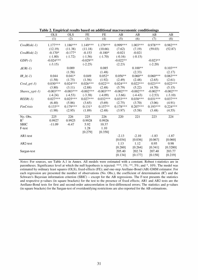
and random effects (RE). Those results are reported in Table 1 (columns 1-6) and Table 2

(columns 1-4). The Arellano-Bond (AB) estimator is then employed to overcome the bias and

inconsistency of the OLS estimation methods (Table 1, columns 7-8; Table 2, columns 5-8).

13

See Arellano and Bond (1991), Blundel and Bond (1998) and Blundell et al. (2000).

16

[Insert Table 1 around here]

[Insert Table 2 around here]

To begin with, two lags of the dependent variable are included in the set of regressors

to capture the effect of possible omitted explanatory variables and the persistence of the credit

risk. The results indicate that there is indeed persistence in the adjustment to the long-run

equilibrium. When random effects are controlled for, only the first lag of the dependent

variable is statistically significant. The FE estimator seems to be the most appropriate –

according to the F-test, Breusch-Pagan Lagrange multiplier test and Hausman test – when the

economic environment is controlled for using the growth rate of real GDP. However, the RE

estimator is preferable when the unemployment variable is used instead (see Table 1). The

inclusion of additional macroeconomic variables makes the pooled-OLS preferable according

to the F-test (see Table 2).14

In any case, the results are quite similar and the coefficient

estimates seem to be robust to these different estimation techniques.

As expected, the results reported in Table 1 indicate that when GDP grows and the

unemployment rate falls the rate of nonperforming loans decreases significantly.15

Looking at

these results from a different perspective, we conclude that the credit risk tends to increase

when the economic environment deteriorates, which is in line with the findings of Salas and

Saurina (2002), Bonfim (2006), Quagliarello (2007), Bohachova (2006), Cifter et al. (2009),

Kattai, (2010) and Louzis et al. (2012). An additional confirmation of that fact is given by the

impact of the financial crisis on the credit risk: during the financial crisis period – here

collected by the dummy FinCrisis – the credit risk has increased substantially.

14

As the number of countries in our sample is lower than the number of variables included in all the estimations

in Table 2, it is not possible to estimate the model controlling for random effects.

15 One lag of GDP and ∆UR are considered to take into account the plausible delay with which economic shocks

affect the likelihood of default and to avoid reverse causality issues and simultaneity problems. As the variable

UR is not stationary, we use its first difference, which provides more consistent and robust estimates. We prefer

to estimate the effects of GDP and ∆UR separately to avoid the bias generated by the strong link between these

two variables. In fact, they are both used as proxies to the economic environment.

17

As mentioned above, to overcome the bias and inconsistency of the OLS estimation

methods, we employ the Arellano-Bond estimator to the data. Four lags of the dependent

variable are used as instruments and the macroeconomic variables are considered as strictly

exogenous since they are all lagged by (at least) one period. This procedure avoids a huge

number of instruments given that we have just five cross-sectional units in the sample. The

consistence of the estimator is assured since the AR tests for serial correlation in the

differenced residuals provide evidence of significant negative first-order autocorrelation but

no evidence of second-order autocorrelation. Moreover, the validity of the instruments used in

this analysis is also confirmed by the Sargan test.

The results reported in Table 1 for the AB estimator are quite interesting because they

reinforce the conclusion that the economic conditions influence greatly the level of credit risk

in the economy. On one hand, a decrease of one percentage point in the growth rate of real

GDP conducts to an immediate increase in the risk of credit of about 0.035 percentage points,

ceteris paribus.16

On the other hand, an acceleration of one point in the unemployment rate

generates an increase of 0.175 percentage points in the rate of nonperforming loans, ceteris

paribus. Our results also show that during the recent financial crises that rate has increased, on

average, by about 0.3 to 0.4 percentage points. Thus, these findings point out to the

importance that economic policies should give to the promotion of growth and employment to

avoid serious problems of credit default and banking crises.

To explore a little more the impact of the macroeconomic environment on the credit

risk, we include in the model some additional variables that can influence it and that can be

controlled more directly by the fiscal and monetary authorities. One important example is the

interest rate as it affects the debt burden and, consequently, the likelihood of a borrower

paying his debt. The long-term interest rate (IR_lt) is used as a benchmark in our analysis

16

The long-run coefficients can be computed dividing each short-run coefficient by one minus the sum of the

coefficients on the lags of the dependent variable; the standard errors can be obtained by the delta method.

18

because most of the loans are usually agreed for a long period of time. The results reported in

Table 2 reinforce the importance of the economic environment and show that higher interest

rates tend to increase the credit risk significantly. This evidence is more robust when the more

adequate and consistent AB estimator is used. In particular, we will rely on the results

provided in columns 7 and 8 because, with the additional macroeconomic conditionings in the

AB estimator, we only need one lag of the dependent variable to account for its persistence.17

Thus, for the interest rate we observe that for each percentage point increase in the

long-term interest rate the rate of nonperforming loans increases by about 0.06 percentage

points, ceteris paribus. This result confirms the important link between the interest rate and

the credit risk pointed out by Nkusu (2011) and Louzis et al. (2012) calls our attention to the

essential role that monetary authorities can play in the stabilization of that risk.

We also consider that when credit expands or grows faster, the risk of more defaults in

the future may increase because that expansion might be achieved at the cost of more risky

loans. As that effect may not be felt immediately, we decided to try several lags of the

quarterly growth rate of the loans provided by banks (Cred_gr) and found that its effect is felt

with more significance three periods after the expansion in the loans granted to the economy.

Moreover, that impact is positive, as expected. This means that a substantial expansion in

credit may reflect that several risky loans are being approved increasing the number of

potential defaults in the future. The role of the regulatory authorities is very important here to

prevent such situations and to supervise whether the prudential rules for granting loans to the

economy are being followed or not.

The annual growth rate of the share price indices (Shares_ygr) is another variable that

we consider in the analysis as an indicator for the state of the economy. In particular, it

provides a general indication of the firms’ financial conditions. The results show that an

17

All the additional macroeconomic regressors are included with (at least) one lag by the same reasons pointed

out above for GDP and ∆UR.

19

increase in the stock prices – that reflect an improvement in the financial conditions –

contributes to a reduction of the rate of nonperforming loans.

The lag of the real effective exchange rate (REER), with reference to the 27 EU

members, is also included in the equation to control for external competitiveness. Our

findings point out to the fact that an increase in this variable contributes to an increase in the

credit risk. In fact, a real appreciation of the local currency reflects the fact that the goods and

services produced in the country are relatively more expensive. This weakens the

competitiveness of export-oriented firms and affects adversely their ability to service their

debts. Consequently, the ratio of nonperforming loans increases. As the countries in our

sample share a single currency – the Euro – that is beyond their control, the only way for

them to achieve a real depreciation is by reducing their costs of production and/or creating the

necessary conditions to increase their productivity levels. This is a strategy that they should

take not only to reduce the credit risk, but also to make their economies more competitive.

The recent financial crisis has exposed several weaknesses and structural problems in

these five economies and our results point out to and additional one: the increase in the credit

risk. Thus, all the structural measures and programmes that can be implemented – and some

are being implemented, especially in those countries that are receiving external financial help

– to promote their external competitiveness, to increase the productivity, to reduce the

external and public debt and to support growth and employment are fundamental to stabilize

their economies. Consequently, the ratio of nonperforming loans may decrease substantially.

5.2. Sensitivity analysis

The variables selected to the empirical analysis presented in the previous sub-section

are considered the most representative of the macroeconomic environment that may influence

the credit risk. In Table 3, we provide a sensitivity analysis where some of those variables are

replaced by other related proxies that try to collect the same kind of effect. We should stress

20

that despite all the experiments made with the (additional) macroeconomic variables, the

effect of the economic environment on the credit risk remains statistically significant.

[Insert Table 3 around here]

We start by replacing the long-term interest rate by the real interest rate (RIR) and by

the spread between the long and short-term interest rates (IR_spd). The coefficients on these

variables remain positive, but only the coefficient on IR_spd is marginally significant. Even

though the results point out in the same direction, the nominal long-term interest rate is more

suitable because most of the loans are usually agreed for a long period of time and economic

agents tend to look at the available nominal rates when they take their decisions.

As the variable Cred_gr does not distinguishes between private and public loans, we

decided to replace this variable by the private and public indebtedness. The private

indebtedness (Indebtness) is measured by the ratio of total private loans to GDP, while the

public indebtedness is proxied by the government public debt as percentage of GDP

(PubDebt).18

The results provided in columns 3 and 4 show that increases in private

indebtedness have the same effect as credit growth. This means that high private debt burdens

make borrowers more vulnerable to adverse shocks affecting their wealth or income, which

raises the chances that they would run into debt servicing problems. However, the level or

even the changes in public debt have not proved to be relevant to the level of credit risk in the

economies considered in our sample.

In regression 5, we replace the annual growth rate in the share price indices by the

respective quarterly growth rate (Shares_qgr), lagged three periods. The results show an

effect that is quite similar to the one found for Shares_ygr. Moreover, they also show that it

takes some time before the changes in the stock market affect the credit risk significantly.

18

As private indebtedness is not stationary, we use its first difference in the model. The coefficient on Indebtness

has also proved to be more statistically significant three periods after its expansion.

21

The terms of trade (TermsTrade) are used in regression 6 instead of REER, but no

significant effects are found for this variable. This might mean that simple nominal changes in

exports relatively to imports are not as relevant to erode borrowers’ profitability or purchasing

power as changes in the real exchange rate.

Inflation is another variable considered in this analysis. However, this variable has no

relevant impact on credit risk. We believe this is the case because inflation not only erodes the

real value of the outstanding loans but also the borrowers’ real income. As one effect is

virtually cancelled by the other, the final impact of the inflation on the credit risk is null.

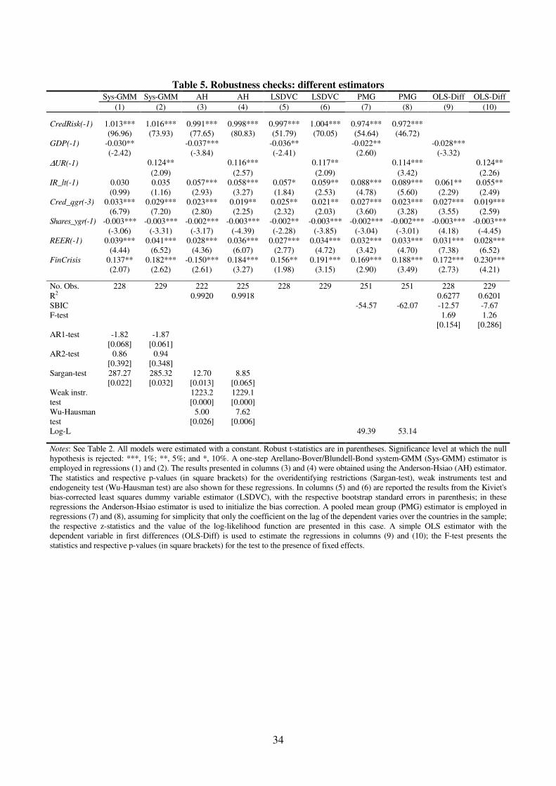
5.3. Robustness checks

To evaluate the robustness of our results to the data and to the estimation procedures,

we provide here an analysis restricting the sample at time and individual levels (Table 4) and

considering other alternative estimators (Table 5).

We start by limiting the sample to the period in which the Euro is in circulation (from

the first quarter of 2001 onwards). The results are not significantly affected with this time-

truncation and the main conclusions remain valid. The same happens when we exclude the

financial crisis period from the sample. Looking at the first four regressions in Table 4, we

observe that only the coefficient on GDP looses its statistical significance with the reduction

of the sample size, but the unemployment rate is still supporting the relevance of the

economic environment on the credit risk (as well as the dummy for the financial crisis).

[Insert Table 4 around here]

In the next step, we decided to exclude a country at a time from the sample. We start

by excluding those countries that are under an external financial help programme (Greece,

Ireland and Portugal); the others (Spain and Italy) are excluded next. In general, the main

findings and conclusions remain unchanged, but there are two results that deserve some

22

consideration. First, the coefficient on GDP is no longer significant when Ireland is excluded

from the sample. This country presents high rates of growth in the 1990s and in the first half

of the 2000s which are linked to lower rates of nonperforming loans. In the second half of the

2000s this relation was inverted, with a substantial decrease in the growth rate of GDP being

followed by an increase in the credit risk. This can be an indication that this country

contributes greatly to the significant negative relation between GDP and CredRisk in our

sample. Second, Portugal, Spain and Italy also contribute significantly to the relation found

between the interest rate and credit risk. When those countries are excluded from the sample

the statistical link between these two variables is not so strong. In fact, the increase in the

interest rates contributed considerably to unveil their weaknesses at the private and public

levels, consequently affecting the credit risk in those economies.

Another set of robustness checks takes into consideration how the data behaves with

regards to different estimators. We consider first the system-GMM estimator. This was

develop by Arellano and Bover (1995) and Blundell and Bond (1998) to solve the problem

that the lagged-level instruments in the AB estimator become weak when the autoregressive

process becomes too persistent or the ratio of the variance of the panel-level effects to the

variance of the idiosyncratic error becomes too large. This estimator considers additional

moment conditions in which lagged differences are used as instruments for the level equation

in addition to the moment conditions of lagged levels as instruments for the differenced

equation. This method assumes that there is no autocorrelation in the idiosyncratic errors and

requires the initial condition that the panel-level effects be uncorrelated with the first

difference of the first observation of the dependent variable.

The results are presented in Table 5 (columns 1 and 2) and show that only the

coefficient on the interest rate has lost its statistical significance. However, this may not be

the most adequate estimator to apply to the available data for the following reasons: first, the

Sargan test clearly rejects the underlying assumptions of the model; second, the coefficient on

23

the lag of the dependent variable is higher than one; third, this estimator is specifically

designed for datasets with many panels and (very) few periods, which is not really the case in

our dataset. Nevertheless, despite all this problems, the main results provided by this

estimator are not very different from the ones obtained with the AB estimator.

[Insert Table 5 around here]

Even though the AB is more efficient than the Anderson-Hsiao (AH) estimator, we

report the results from the AH estimator to check whether the differences in the results are

significant or not. Looking at regressions 3 and 4, we conclude that our findings remain

unchanged. Despite the tests indicating that the instruments used are not weak and the

presence of endogeneity (Wu-Hausman test), the overidentifying restrictions are not valid (see

Sargan test). Hence, it is better to rely on the AB estimator, which is more efficient than this.

An alternative estimation procedure is suggested by Kiviet (1995), especially for small

panels (with a small number of individuals). He derives a formula for the bias of the least-

square dummy variables (LSDV) estimator and recommends subtracting this from the

estimated LSDV coefficients. The estimation of the LSDV correction involves a two-step

procedure in which the residuals from a first-step consistent estimator (for simplicity, we use

the AH estimator) are employed in the second-stage calculation of the bias. Judson and Owen

(1999) notice that the Kiviet's corrected LSDV estimator (LSDVC) can outperform the AB

estimator in some cases. In Monte Carlo experiments they show that its bias tends to be lower

and that it produces the most efficient estimates, especially in small panels. As the number of

individuals in or sample is small, we decided to employ this estimator in the regressions 5 and

6. Once again, the main conclusions of this paper are supported by this alternative estimator.19

19

Although this estimator is theoretically appealing, it is computationally slower to retrieve the results because it

not only involves two estimation steps but also the estimation of bootstrap standard errors. Moreover, it presents

an estimate for the coefficient on the lag of the dependent variable that is almost equal to one, which could point

out to a re-specification of the model with the dependent variable in first differences. We will check this below.

24

With the increase in time observations in a dynamic panel, nonstationarity can be a

concern. Recent papers by Pesaran, Shin, and Smith (1999) offer a different technique to

estimate stationary and nonstationary dynamic panels in which the time (and the number of

groups) is large and some parameters are considered heterogeneous across groups: the pooled

mean-group (PMG) estimator. This estimator relies on a combination of pooling and

averaging of coefficients. Given the advantages of this estimator, we also apply it to our

model constraining the coefficients on the macroeconomic variables to be identical, but

allowing the coefficient on the lag of the dependent variable and the error variances to differ

across groups. Looking at regressions 7 and 8, we conclude that, despite the number of

individuals being small, the results that we get with this estimator are very similar to the ones

obtained with the AB estimator.

A final robustness check takes into account the fact that the coefficient on the lagged

dependent variable is very close to one in the Sys-GMM, AH and LSDVC estimators.

Allowing for the possibility of being equal to one, we transform the model in such a way that

the dependent variable is now the first difference of credit risk (∆CredRisk) and it is a

function of the other regressors. Employing the OLS estimator over this new specification

(called here OLS-Diff), we found no significant differences in the results in comparison with

the other estimators.20

Thus, we conclude that our results and conclusions are robust to different kinds of

estimators. Given their specificities, some are more suitable to our data than others. However,

our preference for the AB estimator in this study is justified by its consistence, efficiency and

reasonable adequacy to the data (as indicated by all diagnostic tests).

20

We are not controlling for fixed effects because the F-test does not reject the simple pooling. Moreover, this

estimator and specification would be very appealing if ∆CredRisk was stationary, but that is not the case. For

example the IPS-test presents a p-value of 0.4699 for ∆CredRisk.

25

6. Conclusions

The recent financial crisis has revived the interest on the analysis of the problems that

banking crises can have over the economy and on the factors that may trigger a banking crisis.

However, before looking at the causes of banking crisis, we should give some attention to the

conditionings of the banking credit risk. In reality, before a banking crisis arises, banks can be

struggling with liquidity and/or insolvency problems caused by the increase of bad or

nonperforming loans in their balance sheets. Thus, to understand the origin of banking crises

it is necessary starting by considering the factors that affect baking credit risk in first place.

Several studies have focused their attention on this matter and have concluded that the

macroeconomic environment has a strong influence on banking credit risk. In this paper, we

analyse deeply the link between the macroeconomics and banking credit risk in the GIPSI.

Employing dynamic panel data approaches to these group countries over the period 1997q1-

2011q3, we conclude that the banking credit risk is significantly affected by the

macroeconomic environment: the credit risk increases when GDP growth and the share price

indices decrease and rises when the unemployment rate, interest rate, and credit growth

increase; it is also positively affected by an appreciation of the real exchange rate; moreover,

we observe a substantial increase in the credit risk during the recent financial crisis period.

Several robustness tests with different estimators have also confirmed these results.

In terms of policy implications, this means that structural measures and programmes

that can be implemented to promote external competitiveness, to increase productivity, to

reduce external and public debt and to support growth and employment in these countries are

fundamental to stabilize their economies.

From this analysis we may think of some interesting avenues for future research. First,

it would be interesting to extend it to other EU countries. The problem is that comparable

aggregate data for credit risk is not always available. Thus, a possible alternative would be to

look at the disaggregated banking level, provided that reliable (and comparable) time series

26

for nonperforming loans are available for the most relevant credit institutions. In this case, in

particular, the group of regressors could be extended with the inclusion of some unsystematic

or microeconomics factors, which will provide a deeper understanding of banking credit risk

as well as additional insights on the link between the recent financial crisis and the risk taken

by some financial and banking institutions. Finally, as the output effects of credit market

frictions could be nonlinear, it may also be worth exploring possible threshold effects.

Acknowledgements

The author wishes to thank the financial support provided by the Portuguese

Foundation for Science and Technology under research grant PEst-C/EGE/UI3182/2011

(partially funded by COMPTE, QREN and FEDER). This article also benefited from the

excellent research assistance of Catarina Sebastião to whom the author is very grateful.

References

Agnello, L., Sousa, R., 2011. How do Banking Crises Impact on Income Inequality? NIPE

Working Papers, WP 30/2011. University of Minho.

Agnello, L., Furceri, D., Sousa, R., 2011. “Fiscal Policy Discretion, Private Spending, and Crisis

Episodes. NIPE Working Papers, WP 31/2011. University of Minho.

Ahmad, N., Ariff, M., 2007. Multi-country study of Bank Credit Risk determinants, International

Journal of Banking and Finance, 5 (1), 135-152.

Ali, A., Daly, K., 2010. Macroeconomic determinants of credit risk: Recent evidence from a cross

country study. International Review of Financial Analysis, 19, 165-171.

Anderson, T., Hsiao, C., 1981. Estimation of dynamic models with error components. Journal of

the American Statistical Association, 76, 598-606.

27

Arellano, M., Bond, S., 1991. Some Tests of Specification for Panel Data: Monte Carlo Evidence

and an Application to Employment Equations. Review of Economic Studies, 58, 277-297.

Athanasoglou, P., Brissimis, S., Delis, M., 2008. Bank-Specific, Industry-Specific and

Macroeconomic Determinants of Bank Profitability. Journal of International Financial

Markets, Institutions and Money, 18 (2), 121-136.

Aver, B., 2008. An Empirical Analysis of Credit Risk Factors of the Slovenian Banking System.

Managing Global Transitions. 6 (3), 317-334.

Baltagi, B., 2008. Econometric Analysis of Panel Data, 4th Ed. Chichester, UK. John Wiley &

Sons, Ltd.

Blundell, R., Bond, S., 1998. Initial Conditions and Moment Conditions in Dynamic Panel Data

Models. Journal of Econometrics, 87, 115-143.

Blundell, R., Bond, S., Windmeijer F., 2000. Estimation in Dynamic Panel Data Models:

Improving on The Performance of the Standard GMM Estimator. in B. Baltagi (ed).

Advances in Econometrics, Volume 15: Non-stationary Panels, Panel Cointegration and

Dynamic Panels, JAI Elsevier Science.

Bohachova, O., 2008. The impact of macroeconomic factors on risks in the banking sector: a

cross-country empirical assessment. IAW Discussion Papers, 44.

Bond, S., 2002. Dynamic Panel Data Models: A Guide to Micro Data Methods and Practice,

Portuguese Economic Journal, 1 (2), 141-162.

Bond, S., Windmeijer, F., 2002. Finite Sample Inference for GMM Estimators in linear Panel Data

Models: A Comparison of Alternative Tests. Mimeo, Institute for fiscal studies, London.

Bonfim, D., 2009. Credit risk drivers: Evaluating the contribution of a firm level information and

macroeconomic dynamics. Journal of Banking and Finance, 33 (2), 281-299

Casu, B., Girardone, C., Molyneuxra, P., 2006. Introducing to banking. USA: Financial

Times Prentice Hall.

28

Cifter, A., Yilmazer, S., Cifter, E., 2009. Analysis of sectoral credit default cycle dependency with

wavelet networks: Evidence from Turkey. Economic Modelling, 26, 1382-1388.

De Grauwe, P., 2008. The banking crisis: Causes, consequences and remedies. University of

Leuven and CESifo. Mimeo.

Demirguç-Kunt, A., Detragiache, E., 1998. The Determinants of Banking Crises and

Developed Countries. IMF Staff Papers, 45 (1), 81-109.

Fainstein, G., Novikov, I., 2011. The Comparative Analysis of Credit Risk Determinants in

the Banking Sector of the Baltic States. Review of Economics and Finance, March 2011.

Festic, M., Kavkler, A., Repina, S., 2011. The macroeconomic sources of systemic risk in the

banking sectors of five new EU member states. Journal of Banking and Finance, 35, 310-322.

Jakubík, P., 2007. Macroeconomic Environment and Credit Risk. Czech Journal of

Economics and Finance, 57 (1-2), 60-78.

Jiménez, G., Saurina, J., 2004. Collateral, type of lender and relationship banking as

determinants of credit risk. Journal of Banking and Finance, 28, 2191-2212.

Jiménez, G., Saurina, J., 2006. Credit cycles, credit risk and prudential regulation.

International Journal of Central Banking, 2 (2), 65-98.

Judson, R., Owen, L., 1999. Estimating Dynamic Panel Data Models: A Guide for

Macroeconomists. Economics Letters, 65, 9-15.

Kattai, R., 2010 Credit risk model for the Estonian banking Sector. Bank of Estonia Working

Papers, 1.

Kiviet, J., 1995. On Bias, Inconsistency, and Efficiency of Various Estimators in Dynamic

Panel Data Models. Journal of Econometrics, 68, 53-78.

Laeven, L., Valencia, F., 2008. Systemic banking crises: A new database. International

Monetary Fund Working Paper 08/224.

Laeven, L., Valencia, F., 2010. Resolution of banking crises: The good, the bad, and the ugly.

International Monetary Fund Working Paper 10/146.

29

Llewellyn, D., 2002. An Analysis of the Causes of Recent Banking Crises. European Journal

of Finance, 8, 152-175.

Louzis, D., Vouldis, A., Metaxas, V., 2012. Macroeconomic and bank-specific determinants

of nonperforming loans in Greece: A comparative study of mortgage, business and

consumer loan portfolios. Journal of Banking and Finance, 36 (4), 1012-1027.

Merkl, C., Stolz S., 2009. Banks Regulatory Buffers, Liquidity Networks and Monetary

Policy Transmission. Applied Economics, 41, 2013-2024.

Nkusu, M., 2011. Nonperforming loans and macrofinancial vulnerabilities in advanced

economies. IMF Working Papers, 161.

Pesaran, M., Shin, Y., Smith, R., 1999. Pooled mean group estimation of dynamic

heterogeneous panels. Journal of the American Statistical Association, 94: 621-634.

Pesola, J., 2005. Banking fragility and distress: An econometric study of macroeconomic

determinants. Bank of Finland Research Discussion Papers, 13/2005.

Quagliarello, M., 2007. Banks’ riskiness over the business cycle: A panel analysis on Italian

intermediaries. Applied Financial Economics, 17, 119-138.

Salas, V., Saurina, J., 2002. Credit risk in two institutional regimes: Spanish commercial and

savings banks. Journal of Financial Services Research, 22 (3), 203-224.

Saunders, A., Cornett, M., 2008. Financial Institutions Management: a Risk Management

Approach. London: McGraw-Hill.

Windmeijer, F., 2005. A Finite Sample Correction for the Variance of Linear Efficient Two-Step

GMM Estimators. Journal of Econometrics, 126 (1), 25-51.

Zribi, N., Boujelbène, Y., 2011. The Factors Influencing Bank Credit Risk: The Case of

Tunisia. Journal of Accounting and Taxation, 3 (4), 70–78.

30

Tables

Table 1. Empirical results based simply on the economic behaviour

OLS OLS FE FE RE RE AB AB

(1) (2) (3) (4) (5) (6) (7) (8)

CredRisk(-1) 1.410*** 1.402*** 1.303*** 1.370*** 0.967*** 0.957*** 1.136*** 1.156***

(14.36) (14.66) (12.52) (11.22) (65.16) (50.07) (11.51) (10.97)

CredRisk(-2) -0.433*** -0.426*** -0.334*** -0.406*** -0.194* -0.217**

(-4.52) (-4.59) (-2.90) (-3.31) (-1.72) (-1.96)

GDP(-1) -0.024** -0.041*** -0.056*** -0.034***

(-2.50) (-3.82) (-4.02) (-2.62)

∆UR(-1) 0.180*** 0.185** 0.291*** 0.174*

(2.93) (2.50) (3.61) (1.92)

FinCrisis 0.225*** 0.245*** 0.196*** 0.271*** 0.291*** 0.428*** 0.308** 0.397***

(3.32) (3.93) (3.37) (4.98) (3.18) (3.26) (2.46) (3.75)

No. Obs. 236 241 236 241 240 246 231 236

R2 0.9912 0.9928 0.9909 0.9927 0.9892 0.9917

SBIC 45.59 38.05 20.25 24.06

F-test 4.99

[0.001]

2.08

[0.084]

LM-test 75.74

[0.000]

4.11

[0.043]

Hausman-test 33.59

[0.000]

3.10

[0.377]

AR1-test -1.91

[0.056]

-1.99

[0.047]

AR2-test 1.58

[0.115]

1.68

[0.092]

Sargan-test 206.75

[0.207]

202.32

[0.345]

Notes: For sources, see Table A.1 in Annex. All models were estimated with a constant. Robust t-statistics are in

parentheses. Significance level at which the null hypothesis is rejected: ***, 1%; **, 5%; and *, 10%. The model was

estimated by ordinary least squares (OLS), fixed-effects (FE); random-effects (RE); and one-step Arellano-Bond (AB)

GMM estimator. For each regression are presented the number of observations (No. Obs.), the coefficient of

determination (R2) and the Schwarz's Bayesian information criterion (SBIC). The F-test presents the statistics and

respective p-values (in square brackets) for the test to the presence of fixed effects; The LM-test is the Breusch-Pagan

test for random effects; The Hausman-test is used to select between a random or a fixed-effects estimator; AR1 and

AR2 tests are the Arellano-Bond tests for first and second-order autocorrelation in first-differenced errors; The

statistics and p-values (in square brackets) for the Sargan-test of overidentifying restrictions are also reported for the

AB estimations.

31

Table 2. Empirical results based on additional macroeconomic conditionings

OLS OLS FE FE AB AB AB AB

(1) (2) (3) (4) (5) (6) (7) (8)

CredRisk(-1) 1.177*** 1.186*** 1.149*** 1.179*** 0.999*** 1.003*** 0.978*** 0.982***

(12.19) (11.38) (11.18) (10.66) (7.62) (7.19) (59.03) (52.87)

CredRisk(-2) -0.170* -0.177* -0.153 -0.180* -0.021 -0.021

(-1.80) (-1.72) (-1.56) (-1.70) (-0.16) (-0.15)

GDP(-1) -0.024*** -0.029** -0.022** -0.023**

(-3.15) (-2.25) (2.23) (-2.20)

∆UR(-1) 0.089 0.085 0.100** 0.103***

(1.58) (1.48) (2.33) (2.17)

IR_lt(-1) 0.044 0.041* 0.049 0.052* 0.056** 0.060** 0.060*** 0.063***

(1.58) (1.75) (1.56) (1.92) (2.49) (2.48) (2.65) (2.61)

Cred_gr(-3) 0.030*** 0.024*** 0.026*** 0.022** 0.024*** 0.022*** 0.023*** 0.022***

(3.80) (3.11) (2.88) (2.48) (5.79) (5.22) (4.70) (5.15)

Shares_ygr(-1) -0.003*** -0.003*** -0.002*** -0.003*** -0.002*** -0.002*** -0.002** -0.002***

(-4.24) (-4.53) (-3.38) (-4.09) (-3.66) (-4-43) (-2.53) (-3.10)

REER(-1) 0.027*** 0.025*** 0.027*** 0.032*** 0.033*** 0.038*** 0.031*** 0.037***

(6.40) (5.86) (3.65) (5.69) (2.75) (3.70) (3.06) (4.91)

FinCrisis 0.133** 0.179*** 0.131* 0.157** 0.178*** 0.207*** 0.193*** 0.224***

(1.98) (2.95) (1.89) (2.48) (3.97) (5.58) (3.48) (4.55)

No. Obs. 225 226 225 226 220 221 223 224

R2 0.9927 0.9925 0.9928 0.9926

SBIC -11.09 -6.47 5.92 10.37

F-test 1.28

[0.279]

1.10

[0.358]

AR1-test -2.13

[0.034]

-2.10

[0.036]

-1.83

[0.067]

-1.87

[0.060]

AR2-test 1.13

[0.260]

1.12

[0.264]

0.95

[0.341]

0.98

[0.3280]

Sargan-test 205.40

[0.134]

202.74

[0.177]

207.40

[0.158]

203.77

[0.219]

Notes: For sources, see Table A.1 in Annex. All models were estimated with a constant. Robust t-statistics are in

parentheses. Significance level at which the null hypothesis is rejected: ***, 1%; **, 5%; and *, 10%. The model was

estimated by ordinary least squares (OLS), fixed-effects (FE); and one-step Arellano-Bond (AB) GMM estimator. For

each regression are presented the number of observations (No. Obs.), the coefficient of determination (R2) and the

Schwarz's Bayesian information criterion (SBIC) – except for the AB regressions. The F-test presents the statistics

and respective p-values (in square brackets) for the test to the presence of fixed effects; AR1 and AR2 tests are the

Arellano-Bond tests for first and second-order autocorrelation in first-differenced errors; The statistics and p-values

(in square brackets) for the Sargan-test of overidentifying restrictions are also reported for the AB estimations.

32

Table 3. Sensitivity analysis

(1) (2) (3) (4) (5) (6) (7) (8)

CredRisk(-1) 0.977*** 0.967*** 0.964*** 0.982*** 0.968*** 0.953*** 0.970*** 0.969***

(56.77) (55.13) (93.12) (55.42) (57.12) (50.82) (68.34) (81.84)

GDP(-1) -0.014* -0.023* -0.025** -0.015**

(-1.78) (-1.75) (-2.46) (-2.11)

∆UR(-1) 0.111** 0.098** 0.164*** 0.085**

(2.30) (2.38) (3.00) (2.22)

IR_lt(-1) 0.045 0.066*** 0.068*** 0.057*** 0.077*** 0.085***

(1.51) (2.77) (3.01) (3.73) (3.06) (3.10)

RIR(-1) 0.033

(1.53)

IR_spd 0.040*

(1.95)

Cred_gr(-3) 0.025*** 0.026*** 0.019*** 0.015*** 0.023*** 0.022***

(5.03) (4.23) (3.62) (3.65) (4.72) (5.19)

∆Indebtness(-3) 0.307** 0.325**

(2.10) (2.01)

PubDebt(-3) 0.006

(0.90)

∆PubDebt(-3) -0.002

(-0.13)

Shares_ygr(-1) -0.003*** -0.003*** -0.002** -0.002*** -0.002** -0.002*** -0.002***

(-3.30) (3.52) (-2.29) (-3.00) (-2.29) (-2.75) (-3.43)

Shares_qgr(-3) -0.004**

(-2.45)

REER(-1) 0.032*** 0.026*** 0.026** 0.033*** 0.030*** 0.035*** 0.037***

(3.02) (9.01) (2.40) (6.65) (2.75) (3.14) (4.06)

TermsTrade(-1) -0.054

(-0.05)

Infl(-1) -0.028 -0.032

(-1.13) (1.19)

FinCrisis 0.190*** 0.245*** 0.128 0.204*** 0.207*** 0.394*** 0.161*** 0.173***

(2.97) (3.89) (1.34) (2.59) (3.01) (6.36) (2.93) (3.37)

No. Obs. 223 224 223 224 223 224 223 224

AR1-test -1.80

[0.071]

-1.88

[0.061]

-1.76

[0.077]

-1.85

[0.0644]

-1.91

[0.055]

-1.91

[0.057]

-1.82

[0.068]

-1.87

[0.062]

AR2-test 0.97

[0.333]

1.10

[0.271]

1.11

[0.265]

1.10

[0.269]

1.14

[0.254]

1.26

[0.208]

0.89

[0.373]

0.91

[0.364]

Sargan-test 212.21

[0.109]

216.40

[0.084]

214.87

[0.087]

207.41

[0.171]

215.31

[0.084]

215.45

[0.091]

206.70

[0.166]

213.24

[0.109]

Notes: See Table 2. All models were estimated with a constant. Robust t-statistics are in parentheses. Significance

level at which the null hypothesis is rejected: ***, 1%; **, 5%; and *, 10%.

33

Table 4. Robustness checks: data

Year>2000 Year>2000 Year<2009 Year<2009 GRC out GRC out IRE out IRE out PRT out PRT out SP, IT out SP, IT out

(1) (2) (3) (4) (5) (6) (7) (8) (9) (10) (11) (12)

CredRisk(-1) 0.985*** 0.987*** 0.972*** 0.973*** 0.973*** 0.981*** 0.972*** 0.972*** 0.976*** 0.985*** 0.965*** 0.982***

(49.94) (44.72) (31.52) (32.90) (55.50) (46.23) (48.42) (48.09) (38.10) (37.71) (33.63) 42.40

GDP(-1) -0.018 -0.017 -0.025** -0.010 -0.021*** -0.035***

(-1.56) (-1.30) (-2.24) (-0.72) (-2.97) (-4.47)

∆UR(-1) 0.112** 0.075*** 0.085* 0.040*** 0.095* 0.116*

(2.28) (4.59) (1.87) (2.76) (1.72) (1.66)

IR_lt(-1) 0.052** 0.059** 0.066** 0.058* 0.141*** 0.136*** 0.069*** 0.073*** 0.069 0.061 0.046 0.050

(2.15) (2.15) (2.04) (1.71) (4.83) (6.27) (2.90) (3.27) (1.49) (1.38) (1.54) (1.40)

Cred_qgr(-3) 0.021*** 0.021*** 0.026** 0.026** 0.024*** 0.022*** 0.029*** 0.028*** 0.025*** 0.025*** 0.019*** 0.021***

(3.50) (3.91) (2.00) (2.15) (2.91) (3.87) (3.68) (4.59) (3.63) (5.07) (3.97) (5.84)

Shares_ygr(-1) -0.003*** -0.003*** -0.002*** -0.002*** -0.001 -0.002** -0.002* -0.002** -0.003*** -0.003*** -0.001 -0.002**

(-4.29) (4.36) (-2.77) (-3.15) (-1.56) (-2.18) (-1.69) (-2.48) (-5.79) (-5.84) (-1.36) (-2.15)

REER(-1) 0.037*** 0.040*** 0.030*** 0.031*** 0.052*** 0.060*** 0.041*** 0.042*** 0.044*** 0.049*** 0.022** 0.035***

(3.52) (6.01) (5.31) (5.32) (3.91) (4.71) (2.82) (3.38) (4.15) (5.11) (2.12) (12.56)

FinCrisis 0.168*** 0.180*** 0.100*** 0.122*** 0.147** 0.162** 0.134** 0.165*** 0.295*** 0.311***

(2.95) (3.73) (2.84) (3.99) (2.20) (2.13) (2.26) (2.86) (4.06) (6.34)

No. Obs. 199 200 172 172 188 189 184 185 170 170 127 128

AR1-test -1.92

[0.055]

-1.96

[0.050]

-1.50

[0.134]

-1.51

[0.132]

-1.60

[0.110]

-1.63

[0.104]

-1.71

[0.087]

-1.71

[0.087]

-1.54

[0.123]

-1.58

[0.114]

-1.66

[0.097]

-1.68

[0.092]

AR2-test 0.66

[0.512]

0.66

[0.507]

0.83

[0.405]

0.81

[0.417]

1.33

[0.1849]

1.31

[0.189]

0.92

[0.358]

0.95

[0.345]

0.45

[0.651]

0.43

[0.671]

0.26

[0.797]

0.30

[0.764]

Sargan-test 197.11

[0.040]

192.29

[0.072]

161.27

[0.183]

160.53

[0.194]

160.06

[0.218]

159.60

(0.243)

160.93

[0.204]

160.53

[0.227]

158.50

[0.082]

157.42

[0.091]

105.90

[0.153]

106.85

[0.155]

Notes: See Table 2. All models were estimated with a constant. Robust t-statistics are in parentheses. Significance level at which the null hypothesis is rejected: ***,

1%; **, 5%; and *, 10%. In regressions (1) and (2) only the period 2001q1-2011q1 is considered. In regressions (3) and (4) the financial crisis period (after 2008q4) is

excluded. In regressions (5) and (6) Greece is excluded from the sample; In regressions (7) and (8) Ireland is excluded from the sample; In regressions (9) and (10)

Portugal is excluded from the sample; In regressions (11) and (12) Spain and Italy are excluded from the sample.

34

Table 5. Robustness checks: different estimators

Sys-GMM Sys-GMM AH AH LSDVC LSDVC PMG PMG OLS-Diff OLS-Diff

(1) (2) (3) (4) (5) (6) (7) (8) (9) (10)

CredRisk(-1) 1.013*** 1.016*** 0.991*** 0.998*** 0.997*** 1.004*** 0.974*** 0.972***

(96.96) (73.93) (77.65) (80.83) (51.79) (70.05) (54.64) (46.72)

GDP(-1) -0.030** -0.037*** -0.036** -0.022** -0.028***

(-2.42) (-3.84) (-2.41) (2.60) (-3.32)

∆UR(-1) 0.124** 0.116*** 0.117** 0.114*** 0.124**

(2.09) (2.57) (2.09) (3.42) (2.26)

IR_lt(-1) 0.030 0.035 0.057*** 0.058*** 0.057* 0.059** 0.088*** 0.089*** 0.061** 0.055**

(0.99) (1.16) (2.93) (3.27) (1.84) (2.53) (4.78) (5.60) (2.29) (2.49)

Cred_qgr(-3) 0.033*** 0.029*** 0.023*** 0.019** 0.025** 0.021** 0.027*** 0.023*** 0.027*** 0.019***

(6.79) (7.20) (2.80) (2.25) (2.32) (2.03) (3.60) (3.28) (3.55) (2.59)

Shares_ygr(-1) -0.003*** -0.003*** -0.002*** -0.003*** -0.002** -0.003*** -0.002*** -0.002*** -0.003*** -0.003***

(-3.06) (-3.31) (-3.17) (-4.39) (-2.28) (-3.85) (-3.04) (-3.01) (4.18) (-4.45)

REER(-1) 0.039*** 0.041*** 0.028*** 0.036*** 0.027*** 0.034*** 0.032*** 0.033*** 0.031*** 0.028***

(4.44) (6.52) (4.36) (6.07) (2.77) (4.72) (3.42) (4.70) (7.38) (6.52)

FinCrisis 0.137** 0.182*** -0.150*** 0.184*** 0.156** 0.191*** 0.169*** 0.188*** 0.172*** 0.230***

(2.07) (2.62) (2.61) (3.27) (1.98) (3.15) (2.90) (3.49) (2.73) (4.21)

No. Obs. 228 229 222 225 228 229 251 251 228 229

R2 0.9920 0.9918 0.6277 0.6201

SBIC -54.57 -62.07 -12.57 -7.67

F-test 1.69

[0.154]

1.26

[0.286]

AR1-test -1.82

[0.068]

-1.87

[0.061]

AR2-test 0.86

[0.392]

0.94

[0.348]

Sargan-test 287.27

[0.022]

285.32

[0.032]

12.70

[0.013]

8.85

[0.065]

Weak instr.

test

1223.2

[0.000]

1229.1

[0.000]

Wu-Hausman

test

5.00

[0.026]

7.62

[0.006]

Log-L 49.39 53.14

Notes: See Table 2. All models were estimated with a constant. Robust t-statistics are in parentheses. Significance level at which the null

hypothesis is rejected: ***, 1%; **, 5%; and *, 10%. A one-step Arellano-Bover/Blundell-Bond system-GMM (Sys-GMM) estimator is

employed in regressions (1) and (2). The results presented in columns (3) and (4) were obtained using the Anderson-Hsiao (AH) estimator.

The statistics and respective p-values (in square brackets) for the overidentifying restrictions (Sargan-test), weak instruments test and

endogeneity test (Wu-Hausman test) are also shown for these regressions. In columns (5) and (6) are reported the results from the Kiviet's

bias-corrected least squares dummy variable estimator (LSDVC), with the respective bootstrap standard errors in parenthesis; in these

regressions the Anderson-Hsiao estimator is used to initialize the bias correction. A pooled mean group (PMG) estimator is employed in

regressions (7) and (8), assuming for simplicity that only the coefficient on the lag of the dependent varies over the countries in the sample;

the respective z-statistics and the value of the log-likelihood function are presented in this case. A simple OLS estimator with the

dependent variable in first differences (OLS-Diff) is used to estimate the regressions in columns (9) and (10); the F-test presents the

statistics and respective p-values (in square brackets) for the test to the presence of fixed effects.

35

Figures

Figure 1. Evolution of the credit risk in the GIPSI

0.0

2.0

4.0

6.0

8.0

10.0

12.0

14.0

16.0

18.0

1997Q

1

1998Q

1

1999Q

1

2000Q

1

2001Q

1

2002Q

1

2003Q

1

2004Q

1

2005Q

1

2006Q

1

2007Q

1

2008Q

1

2009Q

1

2010Q

1

2011Q

1

Year

%

Greece

Ireland

Portugal

Spain

Italy

Sources: See Table A.1 in Annex.

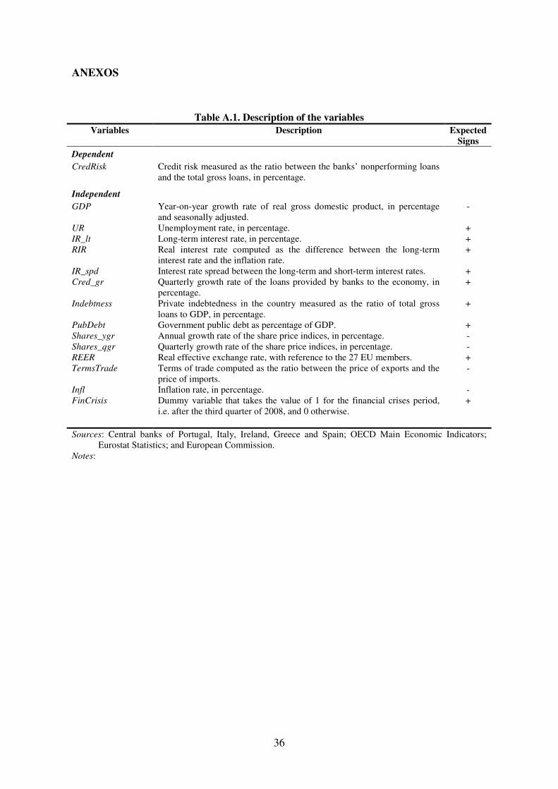
36

ANEXOS

Table A.1. Description of the variables

Variables Description Expected

Signs

Dependent

CredRisk Credit risk measured as the ratio between the banks’ nonperforming loans

and the total gross loans, in percentage.

Independent

GDP Year-on-year growth rate of real gross domestic product, in percentage

and seasonally adjusted.

-

UR Unemployment rate, in percentage. +

IR_lt Long-term interest rate, in percentage. +

RIR Real interest rate computed as the difference between the long-term

interest rate and the inflation rate.

+

IR_spd Interest rate spread between the long-term and short-term interest rates. +

Cred_gr Quarterly growth rate of the loans provided by banks to the economy, in

percentage.

+

Indebtness Private indebtedness in the country measured as the ratio of total gross

loans to GDP, in percentage.

+

PubDebt Government public debt as percentage of GDP. +

Shares_ygr Annual growth rate of the share price indices, in percentage. -

Shares_qgr Quarterly growth rate of the share price indices, in percentage. -

REER Real effective exchange rate, with reference to the 27 EU members. +

TermsTrade Terms of trade computed as the ratio between the price of exports and the

price of imports.

-

Infl Inflation rate, in percentage. -

FinCrisis Dummy variable that takes the value of 1 for the financial crises period,

i.e. after the third quarter of 2008, and 0 otherwise.

+

Sources: Central banks of Portugal, Italy, Ireland, Greece and Spain; OECD Main Economic Indicators;

Eurostat Statistics; and European Commission.

Notes:

37

Table A.2. Descriptive Statistics

Variables Obs. Mean S.D. Min. Max.

CredRisk 251 4.03 3.10 0.70 16.29

GDP 333 2.24 3.06 -8.37 14.45

UR 550 10.22 4.05 3.73 22.20

IR_lt 502 7.98 4.10 3.11 19.03

RIR 482 3.33 2.83 -5.00 14.23

IR_spd 436 1.17 2.32 -13.99 15.05

Cred_gr 461 3.24 2.60 -4.55 20.08

Indebtness 266 4.64 2.21 1.37 9.66

PubDebt 605 72.27 27.66 16.80 142.80

Shares_ygr 416 9.72 35.22 -65.22 286.78

Shares_qgr 431 1.82 12.18 -38.91 82.29

REER 350 103.64 5.29 85.15 120.41

TermsTrade 321 0.99 0.03 0.93 1.11

Infl 635 7.06 6.63 -6.11 32.01

FinCrisis 635 0.09 0.29 0 1

Sources: See Table A.1.

38

Table 3. Correlation Matrix

Variables CredRisk GDP UR IR_lt IR_spd RIR Cred_gr Infl Shares_ygr Shares_mgr PubDebt Indebtness REER TermsTrade FinCrisis

CredRisk 1

GDP -0.3384 1

UR 0.4439 -0.3713 1

IR_lt 0.3612 -0.2116 0.1254 1

IR_spd 0.5253 -0.4622 0.4497 0.5243 1

RIR 0.4919 -0.5863 0.4409 0.3955 0.6176 1

Cred_gr -0.2470 0.4992 -0.3430 0.0008 -0.2127 -0.3898 1

Infl -0.3335 0.5176 -0.4076 0.1213 -0.3797 -0.8637 0.4217 1

Shares_ygr -0.0392 0.5092 -0.0687 -0.2857 -0.1449 -0.1503 0.2690 0.0056 1

Shares_qgr 0.0130 0.1849 0.0307 -0.2357 0.1102 0.1007 0.0462 -0.2382 0.5360 1

PubDebt 0.7444 -0.3226 0.2513 0.2797 0.3458 0.3050 -0.1913 -0.1761 -0.1053 -0.0494 1

Indebtness 0.0382 -0.4461 0.3911 0.0343 0.2476 0.2312 -0.1894 -0.2311 -0.1983 -0.1221 -0.2589 1

REER -0.1726 -0.3735 0.1238 -0.1349 0.1890 0.1433 -0.1732 -0.2290 -0.1654 -0.0644 -0.4591 0.8663 1

TermsTrade 0.0918 -0.0542 -0.0132 -0.0320 0.2213 0.0451 0.1301 -0.0663 0.0667 0.2360 0.0302 -0.1480 -0.0847 1

FinCrisis 0.4007 -0.6848 0.5154 0.2423 0.6627 0.6554 -0.4090 -0.5753 -0.3207 -0.1195 0.2677 0.5673 0.4319 0.0046 1

Sources: See Table A.1.

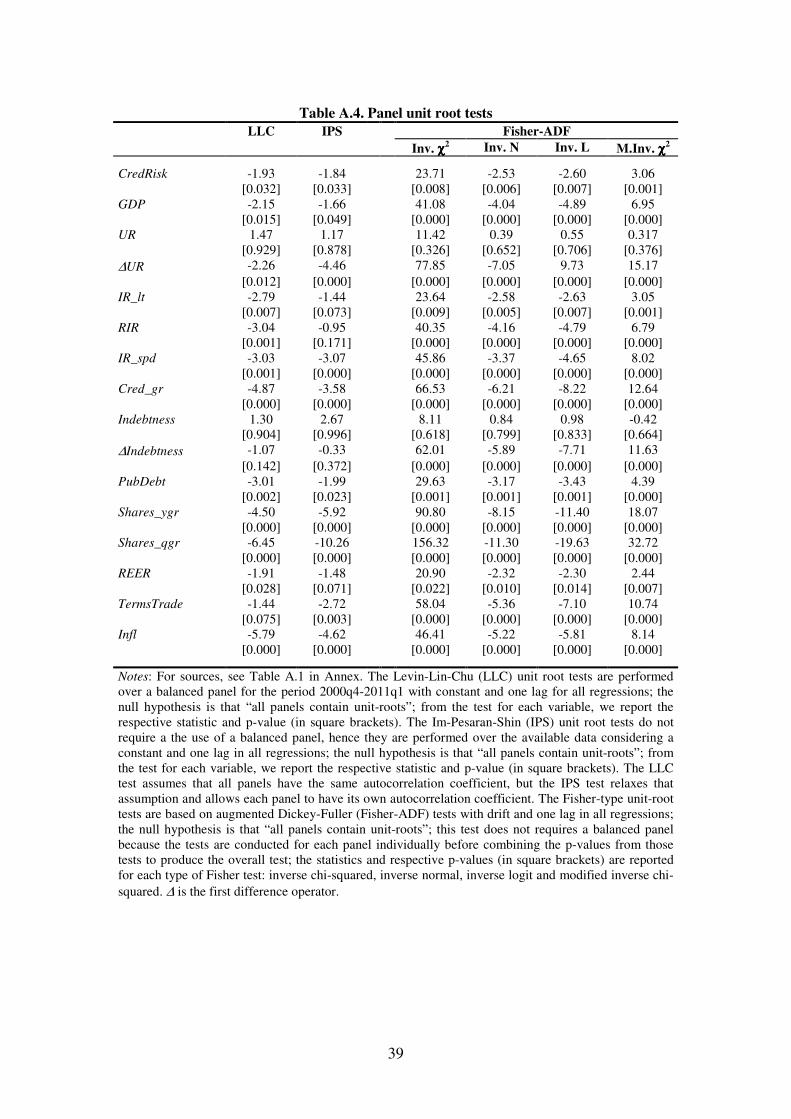
39

Table A.4. Panel unit root tests

LLC IPS Fisher-ADF

Inv. χχχχ

2 Inv. N Inv. L M.Inv. χχχχ2

CredRisk -1.93 -1.84 23.71 -2.53 -2.60 3.06

[0.032] [0.033] [0.008] [0.006] [0.007] [0.001]

GDP -2.15 -1.66 41.08 -4.04 -4.89 6.95

[0.015] [0.049] [0.000] [0.000] [0.000] [0.000]

UR 1.47 1.17 11.42 0.39 0.55 0.317

[0.929] [0.878] [0.326] [0.652] [0.706] [0.376]

∆UR -2.26 -4.46 77.85 -7.05 9.73 15.17

[0.012] [0.000] [0.000] [0.000] [0.000] [0.000]

IR_lt -2.79 -1.44 23.64 -2.58 -2.63 3.05

[0.007] [0.073] [0.009] [0.005] [0.007] [0.001]

RIR -3.04 -0.95 40.35 -4.16 -4.79 6.79

[0.001] [0.171] [0.000] [0.000] [0.000] [0.000]

IR_spd -3.03 -3.07 45.86 -3.37 -4.65 8.02

[0.001] [0.000] [0.000] [0.000] [0.000] [0.000]

Cred_gr -4.87 -3.58 66.53 -6.21 -8.22 12.64

[0.000] [0.000] [0.000] [0.000] [0.000] [0.000]

Indebtness 1.30 2.67 8.11 0.84 0.98 -0.42

[0.904] [0.996] [0.618] [0.799] [0.833] [0.664]

∆Indebtness -1.07 -0.33 62.01 -5.89 -7.71 11.63

[0.142] [0.372] [0.000] [0.000] [0.000] [0.000]

PubDebt -3.01 -1.99 29.63 -3.17 -3.43 4.39

[0.002] [0.023] [0.001] [0.001] [0.001] [0.000]

Shares_ygr -4.50 -5.92 90.80 -8.15 -11.40 18.07

[0.000] [0.000] [0.000] [0.000] [0.000] [0.000]

Shares_qgr -6.45 -10.26 156.32 -11.30 -19.63 32.72

[0.000] [0.000] [0.000] [0.000] [0.000] [0.000]

REER -1.91 -1.48 20.90 -2.32 -2.30 2.44

[0.028] [0.071] [0.022] [0.010] [0.014] [0.007]

TermsTrade -1.44 -2.72 58.04 -5.36 -7.10 10.74

[0.075] [0.003] [0.000] [0.000] [0.000] [0.000]

Infl -5.79 -4.62 46.41 -5.22 -5.81 8.14

[0.000] [0.000] [0.000] [0.000] [0.000] [0.000]

Notes: For sources, see Table A.1 in Annex. The Levin-Lin-Chu (LLC) unit root tests are performed

over a balanced panel for the period 2000q4-2011q1 with constant and one lag for all regressions; the

null hypothesis is that “all panels contain unit-roots”; from the test for each variable, we report the

respective statistic and p-value (in square brackets). The Im-Pesaran-Shin (IPS) unit root tests do not

require a the use of a balanced panel, hence they are performed over the available data considering a

constant and one lag in all regressions; the null hypothesis is that “all panels contain unit-roots”; from

the test for each variable, we report the respective statistic and p-value (in square brackets). The LLC

test assumes that all panels have the same autocorrelation coefficient, but the IPS test relaxes that

assumption and allows each panel to have its own autocorrelation coefficient. The Fisher-type unit-root

tests are based on augmented Dickey-Fuller (Fisher-ADF) tests with drift and one lag in all regressions;

the null hypothesis is that “all panels contain unit-roots”; this test does not requires a balanced panel

because the tests are conducted for each panel individually before combining the p-values from those

tests to produce the overall test; the statistics and respective p-values (in square brackets) are reported

for each type of Fisher test: inverse chi-squared, inverse normal, inverse logit and modified inverse chi-

squared. ∆ is the first difference operator.

Most Recent Working Paper

NIPE WP

11/2012 CCaassttrroo,, VVííttoorr ““ MMaaccrrooeeccoonnoommiicc ddeetteerrmmiinnaannttss ooff tthhee ccrreeddiitt rriisskk iinn tthhee bbaannkkiinngg ssyysstteemm:: TThhee ccaassee

ooff tthhee GGIIPPSSII””,, 22001122

NIPE WP

10/2012 BBaassttooss,, PPaauulloo, NNaattáálliiaa PPiimmeennttaa MMoonntteeiirroo ee OOdddd RRuunnee SSttrraauummee ““PPrriivvaattiizzaattiioonn aanndd ccoorrppoorraattee

rreessttrruuccttuurriinngg””,, 22001122

NIPE WP

09/2012 CCaassttrroo,, VVííttoorr ee RRooddrriiggoo MMaarrttiinnss ““IIss tthheerree dduurraattiioonn ddeeppeennddeennccee iinn PPoorrttuugguueessee llooccaall

ggoovveerrnnmmeennttss’’ tteennuurree??””,, 22001122

NIPE WP

08/2012 MMoonntteeiirroo,, NNaattáálliiaa PPiimmeennttaa ee GGeeooffff SStteewwaarrtt ““ Scale, Scope and Survival: A Comparison of

Labour-Managed, and Capitalist Modes of Production””,, 22001122

NIPE WP

07/2012 AAgguuiiaarr -- CCoonnrraarriiaa,, LLuuííss,, TTeerreessaa MMaarriiaa RRooddrriigguueess ee MMaarriiaa JJooaannaa SSooaarreess ““ Oil Shocks and the

Euro as an Optimum Currency Area””,, 22001122

NIPE WP

06/2012 BBaassttooss,, PPaauulloo,OOdddd RRuunnee SSttrraauummee ee JJaaiimmee AA.. UUrrrreeggoo ““Rain, Food and Tariffs ””,, 22001122

NIPE WP

05/2012 BBrreekkkkee,, KKuurrtt RR..,, LLuuiiggii SSiicciilliiaannii ee OOdddd RRuunnee SSttrraauummee,, ““Can competition reduce quality?””,, 22001122

NIPE WP

04/2012 BBrreekkkkee,, KKuurrtt RR..,, LLuuiiggii SSiicciilliiaannii ee OOdddd RRuunnee SSttrraauummee,, ““Hospital competition with soft

budgets””,, 22001122

NIPE WP

03/2012 LLoommmmeerruudd,, KKjjeellll EErriikk,, OOdddd RRuunnee SSttrraauummee ee SStteeiinnaarr VVaaggssttaadd,, ““ EEmmppllooyymmeenntt pprrootteeccttiioonn aanndd

uunneemmppllooyymmeenntt bbeenneeffiittss:: OOnn tteecchhnnoollooggyy aaddooppttiioonn aanndd jjoobb ccrreeaattiioonn iinn aa mmaattcchhiinngg mmooddeell””,, 22001122

NIPE WP

02/2012

Amado, Cristina e Timo Teräsvirta,, ““MMooddeelllliinngg CChhaannggeess iinn tthhee UUnnccoonnddiittiioonnaall VVaarriiaannccee ooff

LLoonngg SSttoocckk RReettuurrnn SSeerriieess””,, 22001122

NIPE WP

01/2012

Martins, Rodrigo e Francisco José Veiga,, ““ TTuurrnnoouutt aanndd tthhee mmooddeelliinngg ooff eeccoonnoommiicc ccoonnddiittiioonnss::

EEvviiddeennccee ffrroomm PPoorrttuugguueessee eelleeccttiioonnss””,, 22001122

NIPE WP

34/2011

Agnello, L ee RRiiccaarrddoo MM.. SSoouussaa,, ““ Fiscal Consolidation and Income Inequality ””,, 22001111

NIPE WP

33/2011

Maria Caporale, G ee RRiiccaarrddoo MM.. SSoouussaa,, ““Are Stock and Housing Returns Complements or

Substitutes? Evidence from OECD Countries”, 22001111

NIPE WP

32/2011

Maria Caporale, G ee RRiiccaarrddoo MM.. SSoouussaa,, ““Consumption, Wealth, Stock and Housing Returns:

Evidence from Emerging Markets ””,, 22001111

NIPE WP

31/2011

Luca Agnello, Davide Furceri ee RRiiccaarrddoo MM.. SSoouussaa,, ““Fiscal Policy Discretion, Private Spending,

and Crisis Episodes ? ””,, 22001111

NIPE WP

30/2011

Agnello, L ee RRiiccaarrddoo MM.. SSoouussaa,, ““How do Banking Crises Impact on Income Inequality? ””,, 22001111

NIPE WP

29/2011

Alexandre, Fernando, Luís Aguiar-Conraria, Pedro Bação e Miguel Portela, “A Poupança em

Portugal”, 2011

NIPE WP

28/2011

Alexandre, Fernando e Carmen Mendes, “Growth, Consumption and Political Stability in

China”, 2011

NIPE WP

27/2011 BBaalleeiirraass,, RRuuii NNuunnoo,, ““CCoolllleeccttiivvee EEffffiicciieennccyy SSttrraatteeggiieess:: AA RReeggiioonnaall DDeevveellooppmmeenntt PPoolliiccyy

CCoonnttrriibbuuttiioonn ffoorr CCoommppeettiittiivveenneessss EEnnhhaanncceemmeenntt””,, 22001111

NIPE WP

26/2011 BBrreekkkkee,, KKuurrtt RR..,, RRoosseellllaa LLeevvaaggggii,, LLuuiiggii SSiicciilliiaannii ee OOdddd RRuunnee SSttrraauummee,, ““PPaattiieenntt MMoobbiilliittyy,,

HHeeaalltthh CCaarree QQuuaalliittyy aanndd WWeellffaarree””,, 22001111

NIPE WP

25/2011 AAgguuiiaarr -- CCoonnrraarriiaa,, LLuuííss,, PPeeddrroo CC.. MMaaggaallhhããeess ee MMaarriiaa JJooaannaa SSooaarreess ““CCyycclleess iinn PPoolliittiiccss::

WWaavveelleett AAnnaallyyssiiss ooff PPoolliittiiccaall TTiimmee--SSeerriieess””,, 22001111

NIPE WP

24/2011 AAggnneelllloo,,LLuuccaa,, VViittoorr CCaassttrroo ee RRiiccaarrddoo MM.. SSoouussaa ““HHooww DDooeess FFiissccaall PPoolliiccyy RReeaacctt ttoo WWeeaalltthh

CCoommppoossiittiioonn aanndd AAsssseett PPrriicceess?? ””,, 22001111 NIPE WP

23/2011 SSiillvvaa,, HHéélliiaa,, LLiinnddaa VVeeiiggaa ee MMiigguueell PPoorrtteellaa ““SSttrraatteeggiicc IInntteerraaccttiioonn iinn LLooccaall FFiissccaall PPoolliiccyy::

EEvviiddeennccee ffrroomm PPoorrttuugguueessee MMuunniicciippaalliittiieess””,, 22001111

NIPE WP

22/2011 SSoouussaa,, RRiiccaarrddoo MM..,, ““WWeeaalltthh,, LLaabboouurr IInnccoommee,, SSttoocckk RReettuurrnnss aanndd GGoovveerrnnmmeenntt BBoonndd YYiieellddss,, aanndd

FFiinnaanncciiaall SSttrreessss iinn tthhee EEuurroo AArreeaa””,, 22001111

NIPE WP

21/2011 SSoouussaa,, JJooããoo ee RRiiccaarrddoo MM.. SSoouussaa,, ““AAsssseett RReettuurrnnss UUnnddeerr MMooddeell UUnncceerrttaaiinnttyy:: EEvviiddeennccee ffrroomm tthhee

eeuurroo aarreeaa,, tthhee UU..KK.. aanndd tthhee UU..SS.. ””,, 22001111

NIPE WP

20/2011 SSiillaa,, UU ee RRiiccaarrddoo MM.. SSoouussaa,, ““DDoo WWiinnddffaallll GGaaiinnss AAffffeecctt LLaabboouurr SSuuppppllyy?? EEvviiddeennccee ffrroomm tthhee

EEuurrooppeeaann HHoouusseehhoolldd PPaanneell ””,, 22001111