AS-Chap. 3 - 1

R. G

ross

, A. M

arx,

an

dF.

De

pp

e, ©

Wal

the

r-M

eiß

ne

r-In

stit

ut

(20

01

-2

01

3)

Chapter 3

Physics of Josephson Junctions:

The Voltage State

AS-Chap. 3 - 2

R. G

ross

, A. M

arx,

an

dF.

De

pp

e, ©

Wal

the

r-M

eiß

ne

r-In

stit

ut

(20

01

-2

01

3)

For bias currents 𝐼 > 𝐼sm

Finite junction voltage

Phase difference 𝜑 evolves in time: 𝑑𝜑

𝑑𝑡∝ 𝑉

Finite voltage state of the junction corresponds to a dynamic state

Only part of the total current is carried by the Josephson current additional resistive channel capacitive channel noise channel

Key questions

How does the phase dynamics look like?

Current-voltage characteristics for 𝐼 > 𝐼sm?

What is the influence of the resistive damping ?

3. Physics of Josephson junctions: The voltage state

AS-Chap. 3 - 3

R. G

ross

, A. M

arx,

an

dF.

De

pp

e, ©

Wal

the

r-M

eiß

ne

r-In

stit

ut

(20

01

-2

01

3)

At finite temperature 𝑇 > 0

Finite density of “normal” electrons Quasiparticles Zero-voltage state: No quasiparticle current For 𝑉 > 0 Quasiparticle current = Normal current 𝐼N Resistive state

High temperatures close to 𝑇c

For 𝑇 ≲ 𝑇𝑐 and 2Δ 𝑇 ≪ 𝑘𝐵𝑇: (almost) all Cooper pairs are broken up Ohmic current-voltage characteristic (IVC)

𝐼N = 𝐺N𝑉, where 𝐺N ≡1

𝑅Nis the normal conductance

Large voltage 𝑉 > 𝑉g =Δ1+Δ2

𝑒

External circuit provides energy to break up Cooper pairs Ohmic IVC

For 𝑇 ≪ 𝑇c and |V| < Vg

Vanishing quasiparticle density No normal current

3.1 The basic equation of the lumped Josephson junction3.1.1 The normal current: Junction resistance

AS-Chap. 3 - 4

R. G

ross

, A. M

arx,

an

dF.

De

pp

e, ©

Wal

the

r-M

eiß

ne

r-In

stit

ut

(20

01

-2

01

3)

For 𝑇 ≪ 𝑇c and V < 𝑉g

IVC depends on sweep direction and on bias type (current/voltage) Hysteretic behavior Current bias 𝐼 = 𝐼s + 𝐼N = 𝑐𝑜𝑛𝑠𝑡. Circuit model

Equivalent conductance GN at T = 0:

Voltage state

Bias current 𝐼 𝐼s 𝑡 = 𝐼c sin𝜑 𝑡 is time dependent IN is time dependent

Junction voltage 𝑉 =𝐼N

𝐺Nis time

dependent IVC shows time-averaged voltage 𝑉

Current-voltage characteristic

3.1.1 The normal current: Junction resistance

AS-Chap. 3 - 5

R. G

ross

, A. M

arx,

an

dF.

De

pp

e, ©

Wal

the

r-M

eiß

ne

r-In

stit

ut

(20

01

-2

01

3) Finite temperature

Sub-gap resistance 𝑅sg 𝑇 for 𝑉 < 𝑉g 𝑅sg 𝑇 determined by amount of thermally excited quasiparticles

𝑛 𝑇 Density of excited quasiparticles

for T > 0 we get

Nonlinear conductance 𝐺N 𝑉, 𝑇

Characteristic voltage (𝐼c𝑅N-product)

Note: There may be a frequency dependence of the normal channel Normal channel depends on junction type

3.1.1 The normal current: Junction resistance

AS-Chap. 3 - 6

R. G

ross

, A. M

arx,

an

dF.

De

pp

e, ©

Wal

the

r-M

eiß

ne

r-In

stit

ut

(20

01

-2

01

3)

If 𝑑𝑉

𝑑𝑡≠ 0 Finite displacement current

Additional current channel

With 𝑉 = 𝐿c𝑑𝐼s

𝑑𝑡, 𝐼N = 𝑉𝐺N, 𝐼D = 𝐶

𝑑𝑉

𝑑𝑡, 𝐿s =

𝐿c

cos 𝜑 𝐿c and 𝐺N 𝑉, 𝑇 =

1

𝑅N

Josephson inductance

For planar tunnel junction

𝐶 ↔ junction capacitance

3.1.2 The displacement current: Junction capacitance

AS-Chap. 3 - 7

R. G

ross

, A. M

arx,

an

dF.

De

pp

e, ©

Wal

the

r-M

eiß

ne

r-In

stit

ut

(20

01

-2

01

3)

Equivalent parallel 𝐿𝑅𝐶 circuit 𝐿c, 𝑅N, C Three characteristic frequencies

Plasma frequency

𝜔𝑝 ∝𝐽c

𝐶𝐴, where 𝐶𝐴 ≡

𝐶

𝐴is the specific junction capacitance

𝜔 < 𝜔p 𝐼D < 𝐼s

Inductive 𝐿c/𝑅N time constant

Inverse relaxation time in the normal+supercurrent system 𝜔c follows from 𝑉c (2nd Josephson equation) 𝐼N < 𝐼c for 𝑉 < 𝑉c or 𝜔 < 𝜔c

Capacitive 𝑅N𝐶 time constant

𝐼D < 𝐼N for 𝜔 <1

𝜏𝑅𝐶

𝑉c = 𝐼c𝑅N

Characteristic frequencies

3.1.3 Characteristic times and frequencies

AS-Chap. 3 - 8

R. G

ross

, A. M

arx,

an

dF.

De

pp

e, ©

Wal

the

r-M

eiß

ne

r-In

stit

ut

(20

01

-2

01

3)

Quality factor

Limiting cases

𝛽𝐶 ≪ 1 Small capacitance and/or small resistance Small 𝑅N𝐶 time constants (𝜏𝑅𝐶𝜔p ≪ 1)

Highly damped (overdamped) junctions

𝛽𝐶 ≫ 1 Large capacitance and/or large resistance Large 𝑅N𝐶 time constants (𝜏𝑅𝐶𝜔p ≫ 1)

Weakly damped (underdamped) junctions

Stewart-McCumber parameter and quality factor

Stewart-McCumber parameter

(𝑄 compares the decay of oscillation amplitudes to the oscillation period)

3.1.3 Characteristic times and frequencies

AS-Chap. 3 - 9

R. G

ross

, A. M

arx,

an

dF.

De

pp

e, ©

Wal

the

r-M

eiß

ne

r-In

stit

ut

(20

01

-2

01

3)

Fluctuation/noise Langevin method: include random source fluctuating noise current type of fluctuations: thermal noise, shot noise, 1/f noise

Thermal Noise

Johnson-Nyquist formula for thermal noise (𝑘B𝑇 ≫ 𝑒𝑉, ℏ𝜔):

relative noise intensity (thermal energy/Josephson coupling energy):

𝐼𝑇 ≡ thermal noise current𝑇 = 4.2 K 𝐼𝑇 ≈ 0.15 μA

(current noise power spectral density)

(voltage noise power spectral density)

3.1.4 The fluctuation current

AS-Chap. 3 - 10

R. G

ross

, A. M

arx,

an

dF.

De

pp

e, ©

Wal

the

r-M

eiß

ne

r-In

stit

ut

(20

01

-2

01

3)

Shot Noise

Schottky formula for shot noise (𝑒𝑉 ≫ 𝑘B𝑇 𝑉 > 0.5 mV@ 4.2 K):

Random fluctuations due to the discreteness of charge carriers Poisson process Poissonian distribution Strength of fluctuations variance 𝛥𝐼2 ≡ 𝐼 − 𝐼 2

Variance depends on frequency Use noise power:

includes equilibriumfluctuations (white noise)

1/f noise

Dominant at low frequencies Physical nature often unclear Josephson junctions: dominant below about 1 Hz - 1 kHz Not considered here

3.1.4 The fluctuation current

AS-Chap. 3 - 11

R. G

ross

, A. M

arx,

an

dF.

De

pp

e, ©

Wal

the

r-M

eiß

ne

r-In

stit

ut

(20

01

-2

01

3) Kirchhoff‘s law: 𝐼 = 𝐼s + 𝐼N + 𝐼D + 𝐼𝐹

Voltage-phase relation: 𝑑𝜑

𝑑𝑡=

2𝑒𝑉

ℏ

Basic equation of a Josephson junction

Nonlinear differential equation with nonlinear coefficients

Complex behavior, numerical solution

Use approximations (simple models)

Super-current

Normalcurrent

Displace-ment

current

Noise current

3.1.5 The basic junction equation

AS-Chap. 3 - 12

R. G

ross

, A. M

arx,

an

dF.

De

pp

e, ©

Wal

the

r-M

eiß

ne

r-In

stit

ut

(20

01

-2

01

3)

Differential equation in dimesionless or energy formulation

≡ 𝑖 ≡ 𝑖F(𝑡)

with

Tilted washboard potential

Resistively and Capacitively ShuntedJunction (RCSJ) model

Mechanical analogGauge invariant phase difference ↔ Particle with mass M and damping 𝜂 in potential U:

Approximation 𝐺𝑁 𝑉 ≡ 𝐺 = 𝑅−1 = const.𝑅 = Junction normal resistance

3.2 The resistively and capacitively shunted junction (RCSJ) model

AS-Chap. 3 - 13

R. G

ross

, A. M

arx,

an

dF.

De

pp

e, ©

Wal

the

r-M

eiß

ne

r-In

stit

ut

(20

01

-2

01

3)

Normalized time:

Stewart-McCumber parameter:

Plasma frequency

Neglect damping, zero driving and small amplitudes (sin𝜑 ≈ 𝜑)

Solution:

Plasma frequency = Oscillation frequency around potential minimum

Finite tunneling probability:Macroscopic quantum tunneling (MQT)

Escape by thermal activation Thermally activated phase slips

Motion of „phase particle“ 𝜑 in the tilted washboard potential

3.2 The resistively and capacitively shunted junction (RCSJ) model

AS-Chap. 3 - 14

R. G

ross

, A. M

arx,

an

dF.

De

pp

e, ©

Wal

the

r-M

eiß

ne

r-In

stit

ut

(20

01

-2

01

3)

The pendulum analog

Plane mechanical pendulum in uniform gravitational field Mass 𝑚, length ℓ, deflection angle 𝜃 Torque 𝐷 parallel to rotation axis Restoring torque: 𝑚𝑔ℓ sin 𝜃

Equation of motion 𝐷 = 𝛩 𝜃 + 𝛤 𝜃 + 𝑚𝑔ℓ sin 𝜃

Θ = 𝑚ℓ2 Moment of inertiaΓ Damping constant

𝐼 ↔ 𝐷𝐼c ↔ 𝑚𝑔ℓ𝛷0

2𝜋𝑅↔ 𝛤

C𝛷0

2𝜋↔ 𝛩

𝜑 ↔ 𝜃

For 𝐷 = 0 Oscillations around equilibrium with

𝜔 =𝑔

ℓ↔ Plasma frequency 𝜔p =

2𝜋𝐼c

𝛷0𝐶

Finite torque (𝐷 > 0) Finite 𝜃0 Finite, but constant 𝜑0 Zero-voltage stateLarge torque (deflection > 90°) Rotation of the pendulum Finite-voltage state

Voltage 𝑉↔ Angular velocity of the pendulum

Analogies

3.2 The resistively and capacitively shunted junction (RCSJ) model

AS-Chap. 3 - 15

R. G

ross

, A. M

arx,

an

dF.

De

pp

e, ©

Wal

the

r-M

eiß

ne

r-In

stit

ut

(20

01

-2

01

3)

Underdamped junction

𝛽𝐶 =2𝑒𝐼𝑐𝑅

2𝐶

ℏ≫ 1

Capacitance & resistance large𝑀 large, 𝜂 smallHysteretic IVC

Overdamped junction

𝛽𝐶 =2𝑒𝐼𝑐𝑅

2𝐶

ℏ≪ 1

Capacitance & resistance small𝑀 small, 𝜂 largeNon-hysteretic IVC

(Once the phase is moving, the potential has to be tilt back almost into the horizontal position to stop ist motion)

3.2.1 Under- and overdamped Josephson junctions

(Phase particle will retrap immediately at 𝐼c because of large damping)

AS-Chap. 3 - 16

R. G

ross

, A. M

arx,

an

dF.

De

pp

e, ©

Wal

the

r-M

eiß

ne

r-In

stit

ut

(20

01

-2

01

3)

„Applied Superconductivity“ One central question is

„How to extract information about the junction experimentally?“

3.3 Response to driving sources

Typical strategy

Drive junction with a probe signal and measure response

Examples for probe signals

Currents (magnetic fields) Voltages (electric fields) DC or AC Josephson junctions AC means microwaves!

Prototypical experiment

Measure junction IVC Typically done with current bias

Motivation

AS-Chap. 3 - 17

R. G

ross

, A. M

arx,

an

dF.

De

pp

e, ©

Wal

the

r-M

eiß

ne

r-In

stit

ut

(20

01

-2

01

3)

Time averaged voltage:2𝜋

Total current must be constant (neglecting the fluctuation source):

where:

𝐼 > 𝐼c Part of the current must flow as 𝐼N or 𝐼D

Finite junction voltage 𝑉 > 0 Time varying 𝐼s 𝐼N + 𝐼D varies in time Time varying voltage, complicated non-sinusoidal oscillations of 𝐼s,

Oscillating voltage has to be calculated self-consistently Oscillation frequency 𝑓 = 𝑉 𝛷0

𝑇 = Oscillation period

3.3.1 Response to a dc current source

AS-Chap. 3 - 18

R. G

ross

, A. M

arx,

an

dF.

De

pp

e, ©

Wal

the

r-M

eiß

ne

r-In

stit

ut

(20

01

-2

01

3)

For 𝐼 ≳ 𝐼c

Highly non-sinusoidal oscillations Long oscillation period

𝑉 ∝1

𝑇is small

I/Ic = 1.05

I/Ic = 1.1

I/Ic = 1.5

I/Ic = 3.0

Analogy to pendulum

3.3.1 Response to a dc current source

For 𝐼 ≫ 𝐼c

Almost all current flows as normal current Junction voltage is nearly constant Almost sinusoidal Josephson current

oscillations Time averaged Josephson current almost

zero Linear/Ohmic IVC

AS-Chap. 3 - 19

R. G

ross

, A. M

arx,

an

dF.

De

pp

e, ©

Wal

the

r-M

eiß

ne

r-In

stit

ut

(20

01

-2

01

3)

Strong damping

𝛽𝐶 ≪ 1 & neglecting noise current

𝑖 < 1 Only supercurrent, 𝜑 = sin−1 𝑖 is a solution, zero junction voltage𝑖 > 1 Finite voltage, temporal evolution of the phase

Integration using

gives

Periodic function with period

Setting 𝜏0 = 0 and using 𝜏 =𝑡

𝜏c

tan−1 𝑎 tan 𝑥 + 𝑏is 𝜋-periodic

3.3.1 Response to a dc current source

AS-Chap. 3 - 20

R. G

ross

, A. M

arx,

an

dF.

De

pp

e, ©

Wal

the

r-M

eiß

ne

r-In

stit

ut

(20

01

-2

01

3)

with

We get for 𝑖 > 1

and

3.3.1 Response to a dc current source

AS-Chap. 3 - 21

R. G

ross

, A. M

arx,

an

dF.

De

pp

e, ©

Wal

the

r-M

eiß

ne

r-In

stit

ut

(20

01

-2

01

3)

𝜔𝑅𝐶 =1

𝑅N𝐶is very small

Large C is effectively shunting oscillating part of junction voltage 𝑉 𝑡 ≃ 𝑉 Time evolution of the phase

Almost sinusoidal oscillation of Josephson current

Down to 𝑉 ≈ℏ𝜔𝑅𝐶

𝑒≪ 𝑉c = 𝐼c𝑅N

Corresponding current ≪ 𝐼c Hysteretic IVC

Weak damping

𝛽𝐶 ≫ 1 & neglecting noise current

Ohmic result valid for 𝑅N = 𝑐𝑜𝑛𝑠𝑡.

Real junction IVC determined by voltage dependence of 𝑅N = 𝑅N V

3.3.1 Response to a dc current source

AS-Chap. 3 - 22

R. G

ross

, A. M

arx,

an

dF.

De

pp

e, ©

Wal

the

r-M

eiß

ne

r-In

stit

ut

(20

01

-2

01

3)

𝛽𝐶 ≃ 1

Numerically solve IVC General trend

Increasing 𝛽𝐶 ↔ Increasing hysteresis

Hysteresis characterized by retrapping current 𝐼r

𝐼r ∝ washboard potential tilt whereEnergy dissipated in advancing to next minimum = Work done by drive current

Analytical calculation possible for 𝛽𝐶 ≫ 1 (exercise class)

Intermediate damping

Numericalcalculation

3.3.1 Response to a dc current source

𝐼 r/𝐼c

AS-Chap. 3 - 23

R. G

ross

, A. M

arx,

an

dF.

De

pp

e, ©

Wal

the

r-M

eiß

ne

r-In

stit

ut

(20

01

-2

01

3) Phase evolves linearly in time:

Josephson current 𝐼𝑠 oscillates sinusoidally Time average of 𝐼s is zero

𝐼D = 0 since𝑑𝑉dc

𝑑𝑡= 0

Total current carried by normal current 𝐼 =𝑉dc

𝑅N

RCSJ model Ohmic IVCGeneral case 𝑅 = 𝑅N 𝑉 Nonlinear IVC

3.3.1 Response to a dc voltage source

AS-Chap. 3 - 24

R. G

ross

, A. M

arx,

an

dF.

De

pp

e, ©

Wal

the

r-M

eiß

ne

r-In

stit

ut

(20

01

-2

01

3)

Response to an ac voltage source

Weak damping 𝛽𝐶 ≫ 1

Integrating the voltage-phase relation:

Current-phase relation:

Superposition of linearly increasing and sinusoidally varying phase

Supercurrent 𝐼s(𝑡) and ac voltage 𝑉1 have different frequencies Origin Nonlinear current-phase relation

3.3.2 Response to ac driving sources

AS-Chap. 3 - 25

R. G

ross

, A. M

arx,

an

dF.

De

pp

e, ©

Wal

the

r-M

eiß

ne

r-In

stit

ut

(20

01

-2

01

3)

Fourier-Bessel series identity:𝒥𝑛 𝑏 = 𝑛th order Bessel function of the first kind

and:

Ac driven junction 𝑥 = 𝜔1𝑡, 𝑏 =2𝜋

𝛷0𝜔1and 𝑎 = 𝜑0 +𝜔dc𝑡 = 𝜑0 +

2𝜋

𝛷0𝑉dc𝑡

Frequency 𝜔dc couples to multiples of the driving frequency

Imaginary part

Some maths for the analysis of the time-dependent Josephson current

3.3.2 Response to ac driving sources

AS-Chap. 3 - 26

R. G

ross

, A. M

arx,

an

dF.

De

pp

e, ©

Wal

the

r-M

eiß

ne

r-In

stit

ut

(20

01

-2

01

3)

Ac voltage results in dc supercurrent if 𝜔dc − 𝑛𝜔1 𝑡 + 𝜑0 is time independent

Amplitude of average dc current for a specific step number 𝑛

𝑉dc ≠ 𝑉𝑛

𝜔dc − 𝑛𝜔1 𝑡 + 𝜑0 is time dependent Sum of sinusoidally varying terms Time average is zero Vanishing dc component

3.3.2 Response to ac driving sources

Shapiro steps

AS-Chap. 3 - 27

R. G

ross

, A. M

arx,

an

dF.

De

pp

e, ©

Wal

the

r-M

eiß

ne

r-In

stit

ut

(20

01

-2

01

3) Ohmic dependence with sharp current spikes at 𝑉dc = 𝑉𝑛

Current spike amplitude depends on ac voltage amplitude

𝑛th step Phase locking of the junction to the 𝑛th harmonic

Example: 𝜔1/2𝜋 = 10 GHz

Constant dc current at Vdc = 0 and 𝑉𝑛 = 𝑛𝜔1𝛷0

2𝜋≃ 𝑛 × 20 μV

3.3.2 Response to ac driving sources

AS-Chap. 3 - 28

R. G

ross

, A. M

arx,

an

dF.

De

pp

e, ©

Wal

the

r-M

eiß

ne

r-In

stit

ut

(20

01

-2

01

3)

Difficult to solve Qualitative discussion with washboard potential

Increase 𝐼dc at constant 𝐼1 Zero-voltage state for 𝐼dc + 𝐼1 ≤ 𝐼c, finite voltage state for 𝐼dc + 𝐼1 > 𝐼c Complicated dynamics!

𝑉𝑛 = 𝑛𝜔1Φ0

2𝜋Motion of phase particle synchronized by ac driving

Simplifying assumption During each ac cycle phase the particle

moves down 𝑛 minima

Resulting phase change 𝜑 = 𝑛2𝜋

𝑇= 𝑛𝜔1

Average dc voltage 𝑉 = 𝑛𝛷0

2𝜋𝜔1 ≡ 𝑉𝑛

Exact analysis Synchronization of phase dynamics with external ac source for a certain bias current interval

Strong damping 𝛽𝐶 ≪ 1 (experimentally relevant)

Kirchhoff’s law (neglecting ID) 𝐼𝑐 sin 𝜑 +1

𝑅N

𝛷0

2𝜋

𝑑𝜑

𝑑𝑡= 𝐼dc + 𝐼1 sin𝜔1𝑡

3.3.2 Response to ac driving sources

Response to an ac current source

Steps

AS-Chap. 3 - 29

R. G

ross

, A. M

arx,

an

dF.

De

pp

e, ©

Wal

the

r-M

eiß

ne

r-In

stit

ut

(20

01

-2

01

3)

Experimental IVCs obtained for an underdamped and overdamped Niobium Josephson junction under microwave irradiation

3.3.2 Response to ac driving sources

AS-Chap. 3 - 30

R. G

ross

, A. M

arx,

an

dF.

De

pp

e, ©

Wal

the

r-M

eiß

ne

r-In

stit

ut

(20

01

-2

01

3)

Superconducting tunnel junction Highly nonlinear 𝑅 𝑉

Sharp step at 𝑉g =2𝛥

𝑒

Use quasiparticle (QP) tunneling current 𝐼qp 𝑉

Include effect of ac source on QP tunneling

Bessel function identity for 𝑉1-term Sum of terms Splitting of qp-levels into many levels 𝐸qp ± 𝑛ℏ𝜔1Modified density of states!

Tunneling current

Sharp increase of the 𝐼qp 𝑉 at 𝑉 = 𝑉g is broken up into many steps of smaller current

amplitude at 𝑉𝑛 = 𝑉g ±𝑛ℏ𝜔1

𝑒

Model of Tien and Gordon: Ac driving shifts levels in electrode up and down

QP energy: 𝐸qp + 𝑒𝑉1 cos𝜔1𝑡

QM phase factor

3.3.4 Photon-assisted tunneling

AS-Chap. 3 - 31

R. G

ross

, A. M

arx,

an

dF.

De

pp

e, ©

Wal

the

r-M

eiß

ne

r-In

stit

ut

(20

01

-2

01

3)

Example QP IVC of a Nb SIS Josephson junction without & with microwave irradiation Frequency 𝜔1 2𝜋 = 230 GHz corresponding to ℏ𝜔1 𝑒 ≃ 950 μV

Shapiro steps

Appear at 𝑉𝑛 = 𝑛ℏ

2𝑒𝜔1

Amplitude 𝐽𝑛2𝑒𝑉1

ℏ𝜔1

Sharp steps

QP steps

Appear at 𝑉𝑛 = 𝑛ℏ

𝑒𝜔1

Amplitude 𝐽𝑛𝑒𝑉1

ℏ𝜔1

Broadended steps(depending on 𝐼qp 𝑉 )

𝜔1 2𝜋 = 230 GHz

3.3.4 Photon-assisted tunneling

AS-Chap. 3 - 32

R. G

ross

, A. M

arx,

an

dF.

De

pp

e, ©

Wal

the

r-M

eiß

ne

r-In

stit

ut

(20

01

-2

01

3)

Thermal fluctuations with correlation function:

Larger fluctuations

Incease probability for escape out of potential well Escape at rates Gn±1

Escape to next minimum Phase change of 2𝜋

𝐼 > 0 Gn+1 > Gn-1𝑑𝜑

𝑑𝑡> 0

Langevin equation for RCSJ model

Equivalent to Fokker-Planck equation:

Normalized force

Normalized momentum

3.4 Additional topic: Effect of thermal fluctuations

Small fluctuations Phase fluctuations around equilibrium

AS-Chap. 3 - 33

R. G

ross

, A. M

arx,

an

dF.

De

pp

e, ©

Wal

the

r-M

eiß

ne

r-In

stit

ut

(20

01

-2

01

3)

𝜎(𝑣, 𝜑, 𝑡) Probability density of finding system at (𝑣, 𝜑) at time 𝑡

Static solution (𝑑𝜎

𝑑𝑡= 0)

with:

Boltzmann distribution (𝐺 = 𝐸–𝐹𝑥 is total energy, 𝐸 is free energy)

Constant probability to find system in nth metastable state

statistical average of variable 𝑋

3.4 Additional topic: Effect of thermal fluctuations

Small fluctuations

AS-Chap. 3 - 34

R. G

ross

, A. M

arx,

an

dF.

De

pp

e, ©

Wal

the

r-M

eiß

ne

r-In

stit

ut

(20

01

-2

01

3)

Attempt frequency 𝜔A

Weak damping (𝛽𝐶 = 𝜔𝑐𝜏𝑅𝐶 ≫ 1) 𝐼 = 0 𝜔A = 𝜔p (Oscillation frequency in the potential well)

𝐼 ≪ 𝐼c 𝜔A » 𝜔p

3.4 Additional topic: Effect of thermal fluctuations

𝑝 can change in time

for Γ𝑛+1 ≫ Γ𝑛−1 and 𝜔A

Γ𝑛+1≫ 1 𝜔A = Attempt frequency

Amount of phase slippage

Large fluctuations

Strong damping (𝛽𝐶 = 𝜔𝑐𝜏𝑅𝐶 ≪ 1)

𝜔p → 𝜔c (Frequency of an overdamped oscillator)

(underdamped junction)

(overdamped junction)

AS-Chap. 3 - 35

R. G

ross

, A. M

arx,

an

dF.

De

pp

e, ©

Wal

the

r-M

eiß

ne

r-In

stit

ut

(20

01

-2

01

3)

For 𝐸J0 ≫ 𝑘B𝑇 Small escape probability ∝ exp −𝑈0 𝐼

𝑘B𝑇at each attempt

Barrier height: 2𝐸J0 for 𝐼 = 0

0 for 𝐼 → 𝐼c

Escape probability 𝜔A/2𝜋 for → 𝐼cAfter escape Junction switches to IRN

Experiment

Measure distribution of escape current 𝐼M Width 𝛿𝐼 and mean reduction 𝛥𝐼c = 𝐼c − 𝐼M Use approximation for 𝑈0 𝐼 and escape rate

𝜔A/2𝜋 exp −𝑈0 𝐼

𝑘B𝑇

Considerable reduction of Ic when kBT > 0.05 EJ0

3.4.1 Underdamped junctions: Critical current reduction by premature switching

Provides experimental information on real or effective temperature!

AS-Chap. 3 - 36

R. G

ross

, A. M

arx,

an

dF.

De

pp

e, ©

Wal

the

r-M

eiß

ne

r-In

stit

ut

(20

01

-2

01

3)

Calculate voltage 𝑉 induced by thermally activated phase slips as a function of current

Important parameter:

3.4.2 Overdamped junctions: The Ambegaokar-Halperin theory

AS-Chap. 3 - 37

R. G

ross

, A. M

arx,

an

dF.

De

pp

e, ©

Wal

the

r-M

eiß

ne

r-In

stit

ut

(20

01

-2

01

3) Finite amount of phase slippage

Nonvanishing voltage for 𝐼 → 0 Phase slip resistance for strong damping (𝛽𝐶 ≪ 1), for U0 = 2EJ0:

𝐸J0

𝑘B𝑇≫ 1 Approximate Bessel function

or

attempt frequency

Attempt frequency is characteristic frequency 𝜔c

Plasma frequency has to be replaced by frequency of overdamped oscillator:

Washboard potential Phase diffuses over barrier Activated nonlinear resistance

Modified Bessel function

3.4.2 Overdamped junctions: The Ambegaokar-Halperin theory

Amgegaokar-Halperin theory

AS-Chap. 3 - 38

R. G

ross

, A. M

arx,

an

dF.

De

pp

e, ©

Wal

the

r-M

eiß

ne

r-In

stit

ut

(20

01

-2

01

3)

epitaxial YBa2Cu3O7 film on SrTiO3 bicrystalline substrate

R. Gross et al., Phys. Rev. Lett. 64, 228 (1990)Nature 322, 818 (1988)

Example: YBa2Cu3O7 grain boundary Josephson junctions Strong effect of thermal fluctuations due to high operation temperature

3.4.2 Overdamped junctions: The Ambegaokar-Halperin theory

AS-Chap. 3 - 39

R. G

ross

, A. M

arx,

an

dF.

De

pp

e, ©

Wal

the

r-M

eiß

ne

r-In

stit

ut

(20

01

-2

01

3)

Determination of 𝐼c 𝑇 close to 𝑇c

Overdamped YBa2Cu3O7 grain boundary Josephson junction

R. Gross et al., Phys. Rev. Lett. 64, 228 (1990)

thermally activated

phase slippage

3.4.2 Overdamped junctions: The Ambegaokar-Halperin theory

AS-Chap. 3 - 40

R. G

ross

, A. M

arx,

an

dF.

De

pp

e, ©

Wal

the

r-M

eiß

ne

r-In

stit

ut

(20

01

-2

01

3)

3.5 Voltage state of extended Josephson junctions

So far

Junction treated as lumped element circuit element Spatial extension neglected

Spatially extended junctions

Specific geometry as as in Chapter 2 Insulating barrier in 𝑦𝑧-plane In-plane 𝐵 field in 𝑦-direction Thick electrodes ≫ 𝜆L1,2 Magnetic thickness 𝑡𝐵 = 𝑑 + 𝜆𝐿,1 + 𝜆𝐿,2 Bias current in 𝑥-direction

Phase gradient along 𝑧-direction

𝜕𝜑 𝑧,𝑡

𝜕𝑧=

2𝜋

𝛷0𝑡𝐵𝐵𝑦 𝑧, 𝑡

Expected effects

Voltage state 𝐸-field and time-dependence become important Short junction and long junction case

AS-Chap. 3 - 41

R. G

ross

, A. M

arx,

an

dF.

De

pp

e, ©

Wal

the

r-M

eiß

ne

r-In

stit

ut

(20

01

-2

01

3)

Neglect self-fields (short junctions)

𝑩 = 𝑩𝐞𝐱

Junction voltage 𝑉 = Applied voltage 𝑉0 Gauge invariant phase difference:

Josephson vortices moving in 𝑧-direction with velocity

3.5.1 Negligible Screening Effects

AS-Chap. 3 - 42

R. G

ross

, A. M

arx,

an

dF.

De

pp

e, ©

Wal

the

r-M

eiß

ne

r-In

stit

ut

(20

01

-2

01

3)

Long junctions (𝑳 ≫ 𝝀𝐉)

Effect of Josephson currents has to be taken into account Magnetic flux density = External + Self-generated field

with B = 𝜇0H and D = 휀0E:in contrast to static case,

now E/t 0

with 𝐸𝑥 = −𝑉/𝑑, 𝐽𝑥 = −𝐽𝑐 sin𝜑 and 𝜕𝜑/𝜕𝑡 = 2𝜋𝑉/Φ0:

consider 1D junction extending in z-direction, B = By, current flow in x-direction

(Josephson penetration depth)

(propagation velocity)

3.5.2 The time dependent Sine-Gordon equation

AS-Chap. 3 - 43

R. G

ross

, A. M

arx,

an

dF.

De

pp

e, ©

Wal

the

r-M

eiß

ne

r-In

stit

ut

(20

01

-2

01

3)

Time dependentSine-Gordon equation

𝑐 = velocity of TEM mode in the junction transmission line

Example: 휀 ≃ 5 − 10, 2𝜆L

𝑑≃ 50 − 100 𝑐 ≃ 0.1𝑐

Reduced wavelength For f = 10 GHz Free space: 3 cm, in junction: 1 mm

with the Swihart velocity

Other form of time-dependent Sine-Gordon equation

3.5.2 The time dependent Sine-Gordon equation

AS-Chap. 3 - 44

R. G

ross

, A. M

arx,

an

dF.

De

pp

e, ©

Wal

the

r-M

eiß

ne

r-In

stit

ut

(20

01

-2

01

3)

Mechanical analogue

Chain of mechanical pendula attached to a twistablerubber ribbon

Restoring torque 𝜆J2 𝜕

2𝜑

𝜕𝑧2

Short junction w/o magnetic field 2/z2 = 0 Rigid connection of pendula Corresponds to single pendulum

Time-dependent Sine-Gordon equation:

3.5.2 The time dependent Sine-Gordon equation

AS-Chap. 3 - 45

R. G

ross

, A. M

arx,

an

dF.

De

pp

e, ©

Wal

the

r-M

eiß

ne

r-In

stit

ut

(20

01

-2

01

3)

Simple case 1D junction (W ≪ λJ), short and long junctions

Short junctions (L ≪ λJ) @ low damping

Neglect z-variation of 𝜑

Equivalent to RCSJ model for 𝐺N = 0, 𝐼 = 0Small amplitudes Plasma oscillations(Oscillation of 𝜑 around minimum of washboard potential)

Long junctions (L ≫ λJ)

Solution for infinitely long junction Soliton or fluxon

𝜑 = 𝜋 at 𝑧 = 𝑧0 + 𝑣𝑧𝑡goes from 0 to 2𝜋 for −∞ → 𝑧 → ∞ Fluxon (antifluxon: ∞ → 𝑧 → −∞)

3.5.3 Solutions of the time dependent SG equation

AS-Chap. 3 - 46

R. G

ross

, A. M

arx,

an

dF.

De

pp

e, ©

Wal

the

r-M

eiß

ne

r-In

stit

ut

(20

01

-2

01

3)

Pendulum analog Local 360° twist of

rubber ribbon

Applied current Lorentz forceMotion of phase twist (fluxon)

Fluxon as particle Lorentz contraction for vz → c

Local change of phase difference Voltage

Moving fluxon = Voltage pulse

Other solutions: Fluxon-fluxon collisions, …

𝜑 = 𝜋 at 𝑧 = 𝑧0 + 𝑣𝑧𝑡goes from 0 to 2𝜋 for −∞ → 𝑧 → ∞ Fluxon (antifluxon: ∞ → 𝑧 → −∞)

3.5.3 Solutions of the time dependent SG equation

AS-Chap. 3 - 47

R. G

ross

, A. M

arx,

an

dF.

De

pp

e, ©

Wal

the

r-M

eiß

ne

r-In

stit

ut

(20

01

-2

01

3)

Linearized Sine-Gordon equation

𝜑1 = Small deviation Approximation

Substitution (keeping only linear terms):

𝜑0 solves time independent SGE 𝜕2𝜑0

𝜕𝑧2= 𝜆J

−2sin 𝜑0

𝜑0 slowly varying 𝜑0 ≈ 𝑐𝑜𝑛𝑠𝑡.

3.5.3 Solutions of the time dependent SG equation

Josephson plasma waves

AS-Chap. 3 - 48

R. G

ross

, A. M

arx,

an

dF.

De

pp

e, ©

Wal

the

r-M

eiß

ne

r-In

stit

ut

(20

01

-2

01

3)

𝜔 < 𝜔p,J

Wave vector k imaginary No proagating solution𝜔 > 𝜔p,J

Mode propagation Pendulum analogue Deflect one pendulum Relax Wave like excitation𝜔 = 𝜔p,J

Infinite wavelength Josephson plasma wave Analogy to plasma frequency in a metal Typically junctions 𝜔p,J ≃ 10 GHz

For very large 𝜆J or very small I

Neglectsin 𝜑

𝜆J2 term Linear wave equation Plane waves with velcoity 𝑐

=𝜔p2

4𝜋2cos𝜑0

3.5.3 Solutions of the time dependent SG equation

Solution:

Dispersion relation ω(k) :

Josephson plasma frequency

(small amplitude plasma waves)

Plane waves

AS-Chap. 3 - 49

R. G

ross

, A. M

arx,

an

dF.

De

pp

e, ©

Wal

the

r-M

eiß

ne

r-In

stit

ut

(20

01

-2

01

3)

Interaction of fluxons or plasma waves with oscillating Josephson current

Rich variety of interesting resonance phenomena Require presence of 𝑩𝐞𝐱

Steps in IVC (junction upconverts dc drive)

For 𝐵ex > 0

Spatially modulated Josephson currrent density moves at 𝑣𝑧 = 𝑉 𝐵𝑦𝑡𝐵 Josephson current can excite Josephson plasma waves

On resonance, em waves couple strongly to Josephson current if 𝒄 = 𝒗𝒛

Eck peak at frequency:

Corresponding junction voltage:

3.5.4 Resonance phenomena

Flux-flow steps and Eck peak

AS-Chap. 3 - 50

R. G

ross

, A. M

arx,

an

dF.

De

pp

e, ©

Wal

the

r-M

eiß

ne

r-In

stit

ut

(20

01

-2

01

3)

Alternative point of view

Lorentz force Josephson vortices move at 𝑣𝑧 =𝑉

𝐵𝑦𝑡𝐵

Increase driving force Increase 𝑣𝑧 Maximum possible speed is 𝑣𝑧 = 𝑐 Further increase of 𝐼 does not increase 𝑉) Flux flow step in IVC

𝑉ffs = 𝑐𝐵𝑦𝑡𝐵 = 𝑐𝛷

𝐿=

𝜔p

2𝜋

𝜆J

𝐿𝛷0

𝛷

𝛷0

Corresponds to Eck voltage

Traveling current wave only excites traveling em wave of same direction Low damping, short junctions Em wave is reflected at open end Eck peak only observed in long junctions at medium damping when

the backward wave is damped

3.5.4 Resonance phenomena

AS-Chap. 3 - 51

R. G

ross

, A. M

arx,

an

dF.

De

pp

e, ©

Wal

the

r-M

eiß

ne

r-In

stit

ut

(20

01

-2

01

3)

Standing em waves in junction “cavity” at 𝜔𝑛 = 2𝜋𝑓𝑛 = 2𝜋 𝑐

2𝐿𝑛 =

𝜋 𝑐

𝐿𝑛

Fiske steps at voltages for L » 100 μmfirst Fiske step » 10 GHz(few 10s of μV)

Interpretation

Wave length of Josephson current density is 2𝜋

𝑘

Resonance condition 𝐿 = 𝑐

2𝑓𝑛𝑛 =

𝜆

2𝑛 ⇒ 𝑘𝐿 = 𝑛𝜋 or 𝛷 = 𝑛

𝛷0

2

where maximum Josephson current of short junction vanishes Standing wave pattern of em wave and Josephson current match Steps in IVC

Influence of dissipation

Damping of standing wave pattern by dissipative effects Broadening of Fiske steps Observation only for small and medium damping

𝜆/2-cavity

𝜔𝑛 = 𝑛𝜋𝑣ph 𝐿

𝑣ph = Phase velocity

3.5.4 Resonance phenomena

Fiske steps

AS-Chap. 3 - 52

R. G

ross

, A. M

arx,

an

dF.

De

pp

e, ©

Wal

the

r-M

eiß

ne

r-In

stit

ut

(20

01

-2

01

3)

Fiske steps at small damping and/or small magnetic field

Eck peak at medium damping and/or medium magnetic field

For 𝑉 ≠ 𝑉Eck and 𝑉 ≠ 𝑉𝑛 𝐼𝑠 = 𝐼c sin 𝜔0𝑡 + 𝑘𝑧 + 𝜑0 ≃ 0 𝐼 = 𝐼N 𝑉 = 𝑉/𝑅N 𝑉

3.5.4 Resonance phenomena

AS-Chap. 3 - 53

R. G

ross

, A. M

arx,

an

dF.

De

pp

e, ©

Wal

the

r-M

eiß

ne

r-In

stit

ut

(20

01

-2

01

3)

Motion of trapped flux due to Lorentz force (w/o magnetic field) Junction of length L, moving back and forth

Phase change of 4𝜋 in period 𝑇 =2𝐿

𝑣z

At large bias currents (𝑣𝑧 → 𝑐)

𝑉zfs = 𝜑ℏ

2𝑒=4𝜋

𝑇

ℏ

2𝑒=

4𝜋

2𝐿/ 𝑐

ℏ

2𝑒=

ℎ

2𝑒

𝑐

𝐿=𝜔p

𝜋

𝜆J𝐿𝛷0

For 𝑛 fluxons

𝑉𝑛,zfs = 𝑛𝑉𝑧𝑓𝑠 𝑉𝑛,zf𝑠 = 2 × Fiske voltage 𝑉𝑛 (fluxon has to move back and forth)

𝑉ffs = 𝑉𝑛,zfs for 𝛷 = 𝑛𝛷0 (introduce n fluxons = generate n flux quanta)

Example:IVCs of annular Nb/insulator/PbJosephson junction containing adifferent number of trapped fluxons

3.5.4 Resonance phenomena

Zero field steps

AS-Chap. 3 - 54

R. G

ross

, A. M

arx,

an

dF.

De

pp

e, ©

Wal

the

r-M

eiß

ne

r-In

stit

ut

(20

01

-2

01

3)

Voltage state: (Josephson + normal + displacement + fluctuation) current = total current

RCSJ-model (𝐺𝑁 𝑉 = 𝑐𝑜𝑛𝑠𝑡.)

Motion of phase particle in the tilted washboard potential

Equivalent LCR resonator, characteristic frequencies:

Equation of motion for phase difference 𝜑:

Quality factor:

𝑑𝜑

𝑑𝑡=2𝑒𝑉

ℏ

Summary (Voltage state of short junctions)

𝛽𝐶 = Stewart-McCumber parameter

AS-Chap. 3 - 55

R. G

ross

, A. M

arx,

an

dF.

De

pp

e, ©

Wal

the

r-M

eiß

ne

r-In

stit

ut

(20

01

-2

01

3)

IVC for strong damping and 𝛽𝐶 ≪ 1

Driving with 𝑉 𝑡 = 𝑉dc + 𝑉1 cos𝜔1𝑡

Shapiro steps at 𝑉𝑛 = 𝑛𝛷0

2𝜋𝜔1

with amplitudes 𝐼s 𝑛 = 𝐼𝑐 𝒥𝑛2𝜋𝑉1

𝛷0𝜔1

Photon assisted tunneling

Voltage steps at 𝑉𝑛 = 𝑛𝛷0

𝜋𝜔1 due to nonlinear

QP resistance

Summary (Voltage state of short junctions)

Effect of thermal fluctuations

Phase-slips at rate Γ𝑛+1 =𝜔A

2𝜋exp −

𝑈0

kB𝑇

Finite phase-slip resistance 𝑅p even below 𝐼c

Premature switching

AS-Chap. 3 - 56

R. G

ross

, A. M

arx,

an

dF.

De

pp

e, ©

Wal

the

r-M

eiß

ne

r-In

stit

ut

(20

01

-2

01

3)

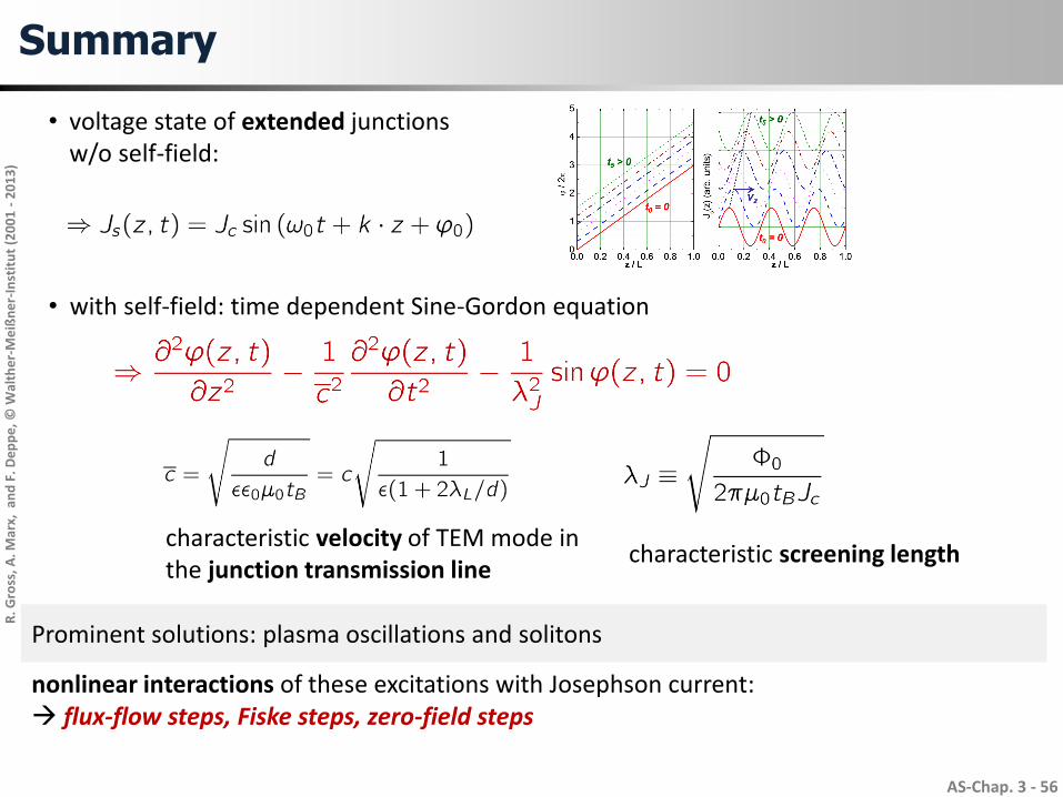
• voltage state of extended junctionsw/o self-field:

• with self-field: time dependent Sine-Gordon equation

characteristic velocity of TEM mode in the junction transmission line

Summary

characteristic screening length

Prominent solutions: plasma oscillations and solitons

nonlinear interactions of these excitations with Josephson current: flux-flow steps, Fiske steps, zero-field steps