7/27/2019 40 Amit Goyal

http://slidepdf.com/reader/full/40-amit-goyal 1/3

 International Journal of Information Technology and Knowledge Management 

 July-December 2012, Volume 5, No. 2, pp. 429-431

1 Department of Electronics and Communication Engineering,

MM University Ambala, India, hodece.sddiet@gmail.com2 Department of Electronics and Communication Engineering,

Lovely Professional University, Phagwara, India,

shaan7_rulez@yahoo.co.in,3 Department of Electronics and Communication Engineering,

Lovely Professional University, Phagwara, India,

kaursimranjeet17@gmail.com

IMPLEMENTATION OF BACK PROPAGATION ALGORITHM

USING MATLAB

Amit Goyal1, Gurleen Kaur Walia2 and Simranjeet Kaur3

 Abstract: Artificial Neural Network (ANN) are highly interconnected and highly parallel systems. Back Propagation is a

common method of training artificial neural networks so as to minimize objective function. This paper describes the

implementation of back propagation algorithm. The error generated at the output is fed back to the input and weights of the

neurons are updated by supervised learning and it is a generalization of delta rule. The sigmoid function is used as a activation

function. The design is simulated using MATLAB R2008a version. Maximum accuracy has been achieved.

 Keywords: Artificial Neural Network, Back Propagation Algorithm, MATLAB.

1. INTRODUCTION

Back Propagation was created by generalising the Widrow-

Hoff learning rule to multiple layer network and non linear

differentiable transfer function. Input vectors and

corresponding target vectors are used to train a network until

it can approximate a function, associate input vectors with

specific output vectors, or classify input vectors in an

appropriate way. Networks with biases, a sigmoid layer and

a linear output layer are capable of approximating any

function with a finite number of discontinuities. Feed

forward networks often have one or more hidden layers of 

sigmoid neurons followed by output layer of linear neurons.

Multiple layers of neurons with non linear transfer functions

allow the network to learn non linear and linear relationshipsbetween input and output vectors. The linear output layer

lets the network produce values outside the range – 1 to +1.

2. SIGMOID ACTIVATION FUNCTION

If we want to constrain the outputs of network between 0

and 1, then the output layer should use a log-sigmoid transfer

function. Before training a feed forward network, the weight

and biases must be initialized. Once the network weights

and biases have been initialized, the network is ready for

training. We used random numbers around zero to initialize

weights and biases in the network. The training process

requires a set of proper inputs and targets as outputs. Duringtraining, the weights and biases of the network are iteratively

adjusted to minimize the network performance function. The

default performance function for feed forward networks is

mean square errors, the average squared errors between thenetwork outputs and the target output. Often the sigmoid

function refers to the special case of the logistic function

and defined by the formula:

1( )

1 x 

 f x e

Figure 1: Sigmoid Function

3. IMPLEMENTATION USING MATLAB

The neural network explained here contains three layers.

These are input, hidden, and output layers. During the

training phase, the training data is fed into the input layer.

The data is propagated to the hidden layer and then to the

output layer. This is called the forward pass of the back

propagation algorithm. In forward pass, each node in hidden

layer gets input from all the nodes from input layer, which

are multiplied with appropriate weights and then summed.

7/27/2019 40 Amit Goyal

http://slidepdf.com/reader/full/40-amit-goyal 2/3

430 INTERNATIONAL JOURNAL OF INFORMATION TECHNOLOGY   AND K NOWLEDGE M ANAGEMENT

The output of the hidden node is the non-linear

transformation of the this resulting sum. Similarly each node

in output layer gets input from all the nodes from hidden

layer, which are multiplied with appropriate weights and

then summed. The output of this node is the non-linear

transformation of the resulting sum. The output values of 

the output layers are compared with the target output values.The target output values are those that we attempt to teach

our network. The error between actual output values and

target output values is calculated and propagated back

towards hidden layer. This is called the backward pass of 

the back propagation algorithm. The error is used to update

the connection strengths between nodes, i.e. weight matrices

between input-hidden layers and hidden-output layers are

updated. During the testing phase, no learning takes place

i.e., weight matrices are not changed. Each test vector is

fed into the input layer. The feed forward of the testing data

is similar to the feed forward of the training data.

The formula for entity synapse s1 is:

*ij ij

m i w

4 j ij

s m

s jis the sum of neurons, m

ijare the intermediate weights,

i is the input to neurons. The waveform for this equation is

shown below:

The formula for entity error generated at output-e1:

=( - )delta *der j j tO O j

Formula for entity neuron n1:

1

1 j sj

Oe

der * (1 ) j j O j

o

Figure 3: Waveform for Entity Neuron n1

Figure 4: Waveform for Entity e1

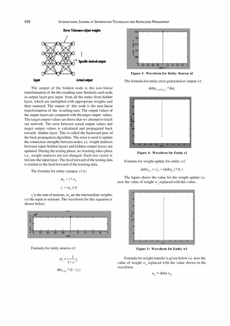
Formula for weight update for entity w1:

delta (delta * )wij ij j

w j O

The figure shows the value for the weight update i.e.

now the value of weight wij

replaced with this value.

Figure 5: Waveform for Entity w1

Formula for weight transfer is given below i.e. now the

value of weight wij

replaced with the value shown in the

waveform.

deltaij ij

w w

7/27/2019 40 Amit Goyal

http://slidepdf.com/reader/full/40-amit-goyal 3/3

IMPLEMENTATION OF B ACK PROPAGATION A LGORITHM USING MATLAB 431

Formula for final weight transfer is:

delta2ij ij

w w

Figure 6: Waveform for Weight Transfer

4. RESULT AND CONCLUSION:

The algorithm is the Error Back propagation learning

algorithm for a layered feed forward network and this

algorithm has many successful applications for trainingmultilayer neural networks. In this paper the last waveform

shows that the weight value becomes constant to minimize

the error at the ouitput. So the output remains constant which

is the objective of this paper.

REFERENCES

[1] I. A. Basheer and M. Hajmeer, “Artificial Neural Networks:

Fundamentals, Computing, Design, and Application”,  J.

 Microbio. Methods, 43, pp. 3-31, Dec. 2000.

[2] Nisha Thomas and Mercy. “Implementation of 

Backpropagation Algorithm in Reconfigurable Hardware”.

2011.

[3] S. Titri, H. Bourmeridja. “New Reuse Design Methodology

for Artificial Neural Network Implementation”. 1999.

[4] Tadayoshi Horita, Takuroa Murata and Itsuo Takanami. “A

Multiple Weight and Neuron Fault Tolerant DigitalMultilayer Neural Network”. 2006.

[5] T. Horita and I. Takanami. “Novel Learning Algorithms

which Make Multilayer Neural Networks Multipleweight-

and-neuron-fault Tolerant”. Proceedings of ICONIP 2005,

pp. 564-569, 2005.

[6] B. Kosko, “Neural Network and Fuzzy System: A

Dynamical Systems Approach to Machine Intelligence”,

Englewood Cliffs, NJ: Prentice-Hall, 1992.

[7] A. Lapedes and R. Farber, “How Neural Networks Works”,

in Neural Information Processing Systems (D.Z. Anderson,

ed.), (Denver), American Institute of Physics, New York,

pp. 442-456, 1988.

[8] R. Linsker, “From Basic Network Principles to NeuralArchitecture”, in Proceedings of the National Academy of 

Sciences, 83,  (USA), pp. 7508-7512, 8390-8394, 8779-

8783, 1986.

[9] M.C. Mozer, “A Focused Back-propagation Algorithm for

Temporal Pattern Recognition”, Complex Systems, 3, pp.

349-381,1989.

[10] G. Wahba, “Generalization and Regularization in Nonlinear

Learning Systems”, in The Handbook of Brain Theory and 

 Neural Networks (M.A. Arbib, ed.), Cambridge, MA: MIT

Press, pp. 426-430, 1995.

[11] H. White, “Learning in Artificial Neural Networks: A

Statistical Perspective”,  Neural Com putation, 1(4), pp.

425-464, 1989.[12] X. Yao, “A New Evolutionary System for Evolving

Artificial Neural Networks”, IEEE Trans. Neural Networks,

8, May 1997.

[13] K.I. Diamantaras and S.Y. Kung, “Principal Component

Neural Networks: Theory and Applications”,  John Wiley

& Sons, 1996.

[14] S.E. Fahlman, “Fast Learning Variations on

Backpropagation: An Empirical Study”, in Proc. 1998

Connectionist Models Summer School (D.S. Touretzky,

G.E. Hinton, and T.J. Sejnowski, eds.), San Mateo, CA:

Morgan Kaufmann, pp. 38-51, 1989.