������������� ���������������������������������� �������������������������������������������������������� ����

�

�

�

�

���� ����������������������

�

�

��

�

�

�������� ������������

�

�

� ���������������!�� �����������������������"�� �������������#������������$���������������� �������������������% ������������������������&������������ ������

�

������'()'��

© Majduline El Haj El Tahir, 2012 Series of dissertations submitted to the Faculty of Mathematics and Natural Sciences, University of Oslo No. 1207 ISSN 1501-7710 All rights reserved. No part of this publication may be reproduced or transmitted, in any form or by any means, without permission. Cover: Inger Sandved Anfinsen. Printed in Norway: AIT Oslo AS. Produced in co-operation with Unipub. The thesis is produced by Unipub merely in connection with the thesis defence. Kindly direct all inquiries regarding the thesis to the copyright holder or the unit which grants the doctorate.

3

����+������������ ���-�������-��������

��������.�� �

�

�

�

�

�

�

�

�

�

�/34567 38�93:�93; <= >456:�?@A 3B >C @D�F?6A 3BG 6I� 3JKL 6I�N6O3P�9 3Q 3R >IG�<?@S3U 6V>W <V>OG� <X>Y@SOG�56Z<[@\6]�56\^93[@S 6R�93; <= >4G 6_�

�

���

�`�bcf^gAkQOG �

�

�

4

m���������Sudan suffers from years of vegetation degradation and is also hit by climate change which has fatal consequences on its fragile economy and the lives of its 41 million people. The vegetation-soil moisture relationships describe the various vegetation patterns which occur in the country. Natural regeneration of Sudan’s vegetation remains the only possible solution for combating this degradation and ultimately contributing to the country’s economic and social stability. In light of these facts the current thesis tries to understand the physical circumstances that impact vegetation regeneration via studying the connections between soil water, erosion and some of the main elements of the hydrological cycle, namely evapotranspiration, temperature and rainfall. The studies of soil moisture and its climatic associations in Sudan are rare especially in the thorough way that is presented here. These results have important food security implications, informing agricultural development, environmental conservation, and water resource planning.

The first stage of this research sought to evaluate the spatial distribution of soil erosion as one of the implications of soil degradation which poses a serious environmental and socioeconomic threat to the environment and to mankind. The developed erosion model used multispectral Advanced Spaceborne Thermal Emission and Reflection Radiometer (ASTER) and Moderate Resolution Imaging Spectroradiometer (MODIS) products from March and December 2006 plus a Shuttle Radar Topography Mission (SRTM) digital elevation model. The results allowed the identification of erosion gullies and subsequent estimation of eroded area. River flow network and slope are identified as more important natural factors, in causing erosion in the Blue Nile region than aspect and elevation.

The second stage concentrated on evaluating evapotranspiration as a direct reflection of the dynamics of soil moisture and hence vegetation regeneration. Both potential and actual evapotranspiration vary from day to day and have a seasonal cycle that determines the rates of vegetative growth and water stress. This thesis, among other, compares three methods for the estimation of daily actual evapotranspiration in Blue Nile. The methods are the remote sensing using the satellite based Surface Energy Balance Algorithm for Land (SEBAL) model with Moderate Resolution Imaging Spectroradiometer (MODIS) satellite data, the modified Thornthwaite water balance method, and the complementary relationship method. A sequence of spatial distribution maps of seasonal actual evapotranspiration are produced. From the maps it was concluded that in the dry season, the spatial distribution pattern is determined by the location, aspect, land use and irrigation activities. In the wet season, the spatial distribution pattern followed that of the rainfall distribution. The seasonal patterns of actual evapotranspiration are a result of the combined effect of rainfall and soil moisture. The seasonal patterns of monthly soil moisture followed those of the monthly rainfall, but with about one month delay in the phase.

The third stage aimed at better understanding the soil moisture variability as a fundamental factor for vegetation regeneration during the period 1965-2005. NCEP/NCAR and PERC reanalysis data are used to study the general trend and to understand the soil moisture, temperature and rainfall relations using Mann Kendall test and geographically weighted regression. To further understand dry and wet variations in terms of regeneration demand, the aridity index is used. The results showed that there are decreasing trends of soil moisture on an annual and seasonal level and that the trend is less dramatic or weaker in the dry season (November-April) than the wet season (May- October). The long-term average of aridity index is affected by the reported decline in rainfall during 1965-1985.

���

�?fopOG����������� ���������������������������������!"�#$����%���������%����&�$'��()����*�%���+���������%(�+�/�����23$�

�����+���46�89���;�<���������=��$���)%%9������>��?���>��4���%@�B"���DE���*��F�/��B"���$%=��G/�����H<����J�����LM���$����%"�Q���R�������;�<�������<������$����$$����%@����2�����<�V�W �X������������������6�89"���%�8���� �Y���

?��F�/X��;�)Z�4X�����$<��$�������$�[X���������Q

��\ )]�����������6�89���� �Y��B"��)^_������� ��$���`�)j���HE���@�)]k��V�����\x�Z����*�<�6�z�B"����4�;����%@������E�)Y����()����*�%���%(�+�/�����V�8<���;�)����+�[;���)#�����23���%[���;�%E����;��"���%�%x)���){�����

|)='��%@�����;�8�k�Q

��()����*�%��+�4�;�(��Z"��$���+�4�;�������;�}�~���<���;��������������%=��$����E��]����(��{�=���;���"�������Z )8����������<�+�4������E���@�)]}k��*�<��x����R����������<��<��;�'���k�(�\"�� ��$%�B"���j���$�����%��;W����%$������x��9��

�%x�$����;��$����%8#�����%���Q�

�B���NO_qG�?;sCVOG��@���*;�����(��()����`)Y�����$���� ������H%%Z�����������<�������$���;�^�����"�����)��()����;�<���B�B"����)%8=��� ��F�/�����%��$�[�����%�%(���� �E��2�� �?����� )��������%���Q�������#�4�(��()����`)Y���4�;������$�) �8��H

�%���F���;�$/k��;�{������x��������������^������ )������ ��='�� �����$�����)Y�$���z�;k���@����) �Z��H��"{���;���;���X�������?)E������j����������'�B����4����;���X��G�[����!�;X������%$<'�)3�k����%�%�8������������$<

Z8������()����`�)Y����G��������������)�(��;�k��2%�����Q�

�+W�;��$�%(?At5vOG�?;sCVOG�B"���%��� ���)������������)#�����H%%Z��()�����*�%��+�%�(��������6�89���� �Y��������Q�������� �����"�#���%"�!�����"$��$���)#�����+�%"$������<��%$4�$����$E��;����'������)=������?)�#����$����+X��������

*�%$����9z��Q��@�)]k��*�<��;�Z��–�|)='�;��'��$z-��) �Z����)]���^��%()#������;�k��2%��������%���"�!��Q

NO_qG�?w\C�OG

�/�8����������������B"���$�� ����$����#�4�(��%���F���;�$/k�����(����;����4X���Z )]Q�

�?At5vOG�?w\C�OG

*�%$��������������$����Z )8��Q�

?vO5vOG�?w\C�OG

�%(��;�Z$�����(��%"��������/������Z )]��H^����3����)8��������B��k���Z )8������#�4����$���� �������x�)=�����"�"4"�!���)#��"�Q����/�$���2�/������$���� �������$�� ����H� �`�!Y���H4������>'�B���2{�����H���x�)#���*�<�V�=����

;���X��G�[��?)����8�'��z�;k�����#�4���Z )]��QZ4�� ������� ���$���� �������$���R��;�8�k��H4�������'��&������;�8�k��&�$k���%$4�$���&�$k���������()����*�%���;�8�k��V�8E���)��$���)%^��"���Y%��<�"�!���)#��"���%$4�$����()����*�%$���������;�8�����%$4�$���&�$k��@���)E��)%=��(Q�

���'?vO5vOG�?;sCVOG�`�E����)%=k��������(��()����*�%��������2��'�HE��B�������<;��%4�4'������)�!���V�=��������6�89���� �Y��M����–��������()����*�%��+�/�����x�F=�HE���������*�Y�X���4�;���2%"���������������)���$���+��%������#������

;�8�k����;�)�����[;����$�����;�8�k���`�!Y���$4����%(�+����=X��HE!��`�!Y���)�_�����#�4��H��+�[�%�@���%@���������6�89"����%�8���� �Y����Q��/������?���=���%$4�$����� �������()����*�%���'�B���)%���+�<�Y������<��'��x������+)E�'�

;�8�k��H4���?��{�=� � ��-�)(���'¡��;�8�k��V�8<��/���(�)^�� �`�!Y���)�_$��2 �8���|�$����4�����'��$�Q�

6

������������Sudan har vært utsatt for flere år med degredasjon av vegetasjonen og er rammet av klimaendringer som har ført til fatale konsekvenser for Sudans skjøre økonomi og livene til landets 41 millioner mennesker. Vegetasjons- og markvannsrelasjoner beskriver de ulike vegetasjonstypemønstre som forekommer i landet. Naturlig regenerering av Sudans vegetasjon er den eneste mulige løsningen for å bekjempe degredasjonen, noe som vil bidra til landets økonomiske og sosiale stabilitet. I lys av disse fakta søker denne avhandlingen å forstå de fysiske forholdene som påvirker vegetasjonsregenerering ved å studere sammenhengene mellom markvann, erosjon og noen av de viktigste elementene i den hydrologiske syklusen, nemlig fordampning, temperatur og nedbør. Undersøkelser av markvann og dets klimatiske avhengigheter er sjeldent i Sudan, spesielt på den grundige måten som er presentert i dette studiet. Disse resultatene har viktige matsikkerhetsimplikasjoner, samt informasjon om relevans for landbruksutvikling, miljøvern og vannressursplanlegging.

I den første fasen av dette studiet ble det søkt å evaluere den romlige fordelingen av jorderosjon som en av konsekvensene av jordforringelse. Videre utgjør dette en alvorlig miljø og sosioøkonomisk trussel mot miljøet og menneskeheten. Den utviklede erosjonsmodellen bruker data fra multispektral Advanced Spaceborne Thermal Emission and Reflection Radiometer (ASTER) og Moderate Resolution Imaging Spectroradiometer (MODIS) produkter fra mars og desember 2006 samt en Shuttle Radar Topography Mission (SRTM) Digital Elevation Model. Resultatene tillot identifisering av eroderte raviner og påfølgende estimering av eroderte områder. Elvesystem og skråninger, fremfor aspekt og høyde, er identifisert som de viktigste naturlige faktorer for erosjon i regionen til den Blå Nilen.

Den andre fasen i dette studiet konsentrerte seg om å vurdere fordampning som en direkte refleksjon av dynamikken i markvann og dermed vegetasjonsregenerasjon. Både potensiell og faktisk fordampning varierer fra dag til dag og har en sesongmessig syklus som bestemmer gradene av vegetativ vekst og vannbehov. Denne avhandlingen sammenligner blant annet tre metoder for estimering av daglig, faktisk fordampning i den Blå Nilen. Metodene er fjernmåling ved hjelp av satellittbasert Surface Energy Balance Algorithm for Land (SEBAL) modell samt Moderate Resolution Imaging Spectroradiometer (MODIS) satellittdata, den modifiserte Thornthwaite vannbalansenmetoden, og komplementær-forholdmetoden. En sekvens av romlige distribusjonskart av en sesongs faktiske fordampning blir produsert. Fra kartene ble det konkludert med at i den tørre årstiden er det romlige fordelingsmønsteret bestemt av plassering, aspekt, arealbruk og bruken av vanningsanlegg. I den våte sesongen fulgte det romlige fordelingsmønsteret nedbørsfordelingen. Det sesongmessige mønsteret av faktisk fordampning er et resultat av den kombinerte effekten av nedbør og markvann. De sesongmessige mønstre av månedlig markvann fulgte de av den månedlige nedbøren, men med omtrent en måneds forsinkelse i fasen.

Den tredje fasen var rettet mot en bedre forståelse av markvannsvariabiliteten som en grunnleggende faktor for vegetasjon regenerering i perioden 1965-2005. NCEP /NCAR og PERC reanalysedata brukes til å studere den generelle trenden, og til å forstå markvann, temperatur og nedbørsrelasjoner ved hjelp av Mann Kendall testen og geografisk vektet regresjon. En tørke indeksen brukes til ytterligere å forstå tørre og våte variasjoner i form av vegetasjonsregenerering etterspørselen. Resultatene viste at det er avtagende trender for markvann på et årlig og sesongmessige nivå og at trenden er svakere i den tørre årstiden (november-april) enn den våte sesongen (mai-oktober). Den langsiktige gjennomsnitts tørkeindeksen blir påvirket av den rapporterte nedgangen i nedbøren i løpet av 1965-1985.�

7

m�.��x������������First and foremost my gratitude is extended to my supervisor Prof. Chong-Yu Xu for his thorough supervision and patient teaching. To him I feel truly indebted for all the hours he spent explaining to me about the different aspects of hydrology. My co-supervisors Prof. Andreas Kääb and Prof. Lars Gottschalk, have helped me with developing an understanding of statistics and remote sensing. Prof. Lena Tallaksen and Prof. Nils Roar Sælthun for their moral back-up and assistance with administrative matters.

As for my collaborators in Sudan I would like to thank Prof. Gamal Al Din Mortada Abdu, Prof. El Nour Abdullah El Siddig and Prof. Osman Mirghani Ali from University of Khartoum and my former colleague Mrs. Dina Abdin Ahmed Salama for their helpful company during the field work in Khartoum, Wad Medani, Singa, Sinnar, and Ad’Damazin. I would also like to thank Dr. Ahmed Abdul Karim, from the Meteorological office in Khartoum and Prof. Kamal Al Din Bashar from the UNESCO Chair-Sudan for providing some of the data and background information upon which this research work is conducted.

From Forskerforbundet I would like to thank Bjarne and Kari Meidell, Live Rasmussen, Torill Marie Rolfsen and Kristian Mollestad. From university of Bergen I would like to thank Prof. Anders Lundberg and Prof. Terje Tveit for all their support for the Norwegian Research Council project # 171783 Modelling and Mapping of Potential Vegetation Regeneration Areas in Sudan using Hydrological Models and Remote Sensing.

My colleagues in Statkraft Energy have facilitated the time and resources for me to complete the final stages of this thesis. Thanks to Gaute Lappegard for checking the Norwegian summary of the thesis.

I would like to thank Dominic O’Fahey for proof reading and linguistical corrections of the thesis and subsequent research publications. To Siza El Haj El Tahir for editing the Arabic summary.

Lastly, I would like to thank my family and friends for their love and encouragement. My friends Hanan Tag El Sir El Safi and Dr. Ahmed Elmokasfi kindly supported me.

My late mother, Suad Khalifa Khogali raised me with a love for challenges and gave me the self confidence to always try and push open new doors. My late father, advocate El Haj El Tahir Ahmed whom I lost at a tender age, continued to enlighten my life through the legacy which he left behind for his love for knowledge and education. My father-in-law Prof. R.S. O’Fahey has tirelessly discussed and outlined the historical and political dimensions of my research through his profound understanding of my home country Sudan. My brothers Khalid and Ayman and my sisters Siza, Dr. Yasmeen, Dr. Safinaz and Sara made my life happier through their respect and understanding. My husband Dominic O’Fahey faithfully supports me in all my pursuits. My children Bushra, Suad and Dalia are a source of inspiration for me and from whom I draw strength to continue working hard.

Thank you all.

Majduline El Haj El Tahir

University of Oslo

March 2012

8

���������y����������������������� � � � � � � � � � z�

{�������������������������� � � � � � � � )(�

)^ +����� ������� � � � � � � � � � )'�

)^)^ |��.��� ���������������x��.�� � � � � � � )'�

)^'^ �������������������� � � � � � � � )}�

)^~^ �������������������������x��.�� � � � � � � )}�

'^ �� ������� � � � � � � � � � '(�

'^)^ m�� ��� ���� � � � � � � � � '(�

'^'^ {���������������������������������� � � ��� � � '���

~^ ��������� � � � � � � � � � � '��

~^)^ ����������������������� � � � � � � � '��

~^'^ ���������������������������������������� � � � � � ~(�

~^~^ �������������������� � � � � � � � ~~�

�^ ��� ������������ ������� � � � � � � � � ~��

�^)^ &�����+� � � � � � � � � � ~��

�^'^ &�����++� � � � � � � � � � ~z�

�^~^ &�����+++� � � � � � � � � � �)�

}^ y���� ���������������������� �� �� � � � � � ���

�^ ����������� � � � � � � � � � �}�

�^ &���������x���������� � � � � � � � � }'�

�^)^ �������&������ � � � � � � � � }~�

�^'^ m��������������������������� � � � � � � ))��

�

�

�

�

9

���������������This thesis is a contribution to project number 171783 “Modelling and Mapping of Potential Vegetation Regeneration Areas in Sudan using Hydrological Models and Remote Sensing”. Project number 171783 is sponsored by the Norwegian Research Council (NFR) and is conducted in collaboration between University of Oslo, Univeristy of Kharoum and University of Bergen. As part of the project, I have contributed to a total of five publications, all listed below. However, only the first three papers whereby I am the first co-author, are defended in this thesis. The other two papers whereby I am the third co-author, are added at the end of this thesis for the purpose of providing further background information about the study. All five papers are referred to in the text by their Roman numerals.

Main defence papers:-

I. �����������������., Kääb, A., and Xu, C-Y (2010). Identification and mapping of soil erosion areas in the Blue Nile, Eastern Sudan using multispectral ASTER and MODIS satellite data and the SRTM elevation model, Hydrology and Earth Systems Science, V14, nr 7, pp 1167–1178.

II. ��� ���� ��� ������ �^ Wenzhong, W.Z., Xu, C-Y, Zhang, Y.J., Singh, VP. (2012). Comparison of methods for estimation of regional actual evapotranspiration in data scarce regions: The Blue Nile region-Eastern Sudan. Journal of Hydrologic Engineering, doi:10.1061/(ASCE)HE.1943-5584.0000429.

III. ��� ���� ��� ������ �^ Xu, C.-Y., and Zengxin Zhang (2012). Soil moisture characteristics and implication for vegetation regeneration in Sudan during the period 1965-2005. Submitted to Journal of Stochastic Environmental Research and Risk Assessment.

In paper I, I was responsible for collecting the field data, remote sensing analyses, writing the draft and final versions of the paper. In paper II, the remote sensing and water balance calculations were made jointly by Wenzhong Wang and I. I was responsible for plotting the results, writing the draft as well as the final version of the paper. In paper III, I was responsible for downloading the data, analysis, draft and final paper-writing.

Additional reference papers:-

IV. Xu, C-Y; Zhang, Q; �����������������. and Zhang, ZX (2010). Statistical properties of the temperature, relative humidity, and net solar radiation in the Blue Nile-eastern Sudan region, Journal of Theoretical and Applied Climatology, V101, nr 3-4, pp 397-409.

V. Zhang, ZX, Xu, C-Y, �����������������^ Cao, JR, Singh, VP. (2012). Spatial and temporal variation of precipitation in Sudan and their possible causes during 1948-2005. Stochastic Environment and Risk Analysis, 26(3): 429–441.

�

�

10

�

{��������������������������a.s.l Above sea level

AE Actual evapotranspiration

AI Aridity index

ASTER Advanced Spaceborne Thermal Emission and Reflection Radiometer

BCM Billion Cubic Meters

CAMS Climate Anomaly Monitoring System

CPA Comprehensive Peace Agreement

DEM Digital elevation model

ECMWF/ERA-40 The European Centre for Medium-Range Weather Forecasts

ENSO El Niño–southern oscillation

ET Evapotranspiration

EVI Enhanced vegetation index

FAO Food and agriculture organization

FCC False colour composites

GCP Ground control point

GG Granger and Gray complementary relationship method

GIS Geographical information systems

GWR Geographically weighted regression

Haboob Dust storm

Hashab The gum arabic tree (Acacia senegal)

ITCZ Intertropical Convergence Zone

Jabal Arabic word for mountain

JRA-25 Japanese reanalysis,

Kerib Bad lands

11

Khor A gully or a seasonal water course

LAI Leaf area index

MERRA Modern Era Retrospective-analysis for Research and Applications

MK Mann Kendall

MLC Maximum likelihood classifier

MODIS Moderate Resolution Imaging Spectroradiometer

NADIR The downward-facing viewing geometry of an orbiting satellite

NASA National Aeronautics and Space Administration

NCEP/NCAR National Centers for Environmental Prediction/National Centre for Atmospheric Research

OLS Ordinary Least Square

PE Reference evapotranspiration

PREC Precipitation REConstructed

RMSE Root Mean Square Error

RS Remote sensing

SEBAL Surface Energy Balance Algorithm for Land

SM Soil moisture

SRTM Shuttle Radar Topography Mission

SST Sea Surface Temperature

SSTA Sea Surface Temperature Anomalies

SWIR Short-wave infrared

SWIR Short-wave infrared

TIR Thermal infrared

VI Vegetation indices

VNIR Visible and near infrared

VNIR Visible and near infrared

WB Thornthwaite water balance model

12

)^ +����� ������

)^)^ |��.��� ���������������x��.�The spatial and temporal distribution of soil moisture is a critical part for many disciplines including agriculture, forest ecology, hydroclimatology, civil engineering, water resources, and ecosystem modelling. Despite its importance, long-term soil moisture data are rare because many soil water sampling techniques are expensive, labour-intensive and difficult to learn without appropriate training (Hymer et al., 2000). This is particularly true in data-scarce places like Sudan. Sudan is suffering from rainfall deficit and water shortages. Delayed arrival of the south-westerly flow and associated rainfall often impose great loss of human lives and economy and has disastrous consequences. With much of rural Africa already struggling to obtain adequate fresh water supplies, the drier conditions and altered precipitation patterns mean that meeting the water needs of the poorest in African is much harder. Considerable literature (Thornes, 1990; Ayoub, 1998; Nakileza et al., 1999; Symeonakis and Drake, 2004) points to the widespread natural resource degradation especially in sub-Saharan Africa, including Sudan. Soil erosion results in the loss of soil nutrients, particularly carbon and nitrogen (West, 1991; Mokwunye, 1996), due to the restrictions of feedbacks in carbon and nitrogen cycles between plants, atmosphere and soil (Schlesinger et al., 1990). Often the equilibrium between the vegetation and the environment is delicate and easily displaced due to climate change or interference of man, leading to the destruction of the pattern and the establishment of more xerophytic vegetation. Drought implies some form of moisture deficit and moisture plays an important role in understanding climate change. Therefore the currently well-evidenced global warming is expected to alter the hydrological cycle, and previous studies tend to provide more observed evidences for this viewpoint (e.g., Beniston and Stephenson 2004; Brutsaert 2006; Zhang et al. 2008). Several observational studies, using meteorological data, point to the climate change in Sudan and these studies confirm that the temperature is rising and rainfall has declined in the past decades which might accelerate environmental degradation and desertification (e.g., Alvi, 1994; Janowiak, 1988; Nicholson et al., 2000; Xu et al., 2010; Zhang et al., 2012).

The vegetation-soil moisture relationships describe the various vegetation patterns which occur in Sudan (Wickens and Collier, 1971). These patterns occur in a variety of soils developed from different parent materials. Chemical differences between the vegetated and non-vegetated areas are not significant and the controlling factor is soil moisture. The soils under the vegetation are more permeable to water than the soils in the intervening non-vegetated areas. The infiltration and retention of moisture is determined by the soil type and the character and arrangement of the soil horizons is of prime importance. The retention of a loose sandy surface is very important since it promotes the infiltration of water to the deeper horizons and later, when the surface dries out during drought, it acts as mulch and prevents water loss by reducing capillary movement.

13

Rainfall is the most important water resource in Sudan and rain-fed agriculture produces food for 90% of the population. Comprehensive analysis and reviews of rainfall trends and variability in Africa, including the Sahel region and Sudan had been carried out by Hulme and his co-authors (e.g., Trilsbach and Hulme, 1984; Hulme, 1987; Hulme and Tosdevin, 1989; Hulme, 1990; Walsh et al., 1988). Trilsbach and Hulme (1984) examined rainfall changes and their physical and human implications in the critical desertification zone in the North and concluded that heavy falls of rain ( > 40 mm) are more likely to decline than medium (> 10 mm) and light (< 10 mm) falls. Walsh et al. (1988) reported that “rainfall decline in semi-arid Sudan since 1965 has continued and intensified in the 1980s, with 1984 the driest year on record and all annual rainfalls from 1980 to 1987 well below the long-term mean”. Hulme (1990) reported that rainfall depletion has been most severe in semi-arid central Sudan between 1921-50 and 1956-85. Similar results are also reported by Eltahir (1992) and Zhang et al. (2012). The length of the wet season has contracted, and rainfall zones have migrated southwards. A reduction in the frequency of rain events rather than a reduced rainfall yield per rain event was found to be the main reason for this depletion. Increasingly the tendency has been for studies examining the causes of droughts, to look at global scales through the notion of teleconnections. The precipitation anomaly of Sudan has been related to Sea Surface Temperature Anomalies (SSTAs) in the Gulf of Guinea (Lamb, 1978a, b). Palmer (1986) has pointed out that the tropical Indian Ocean Sea surface temperature (SST) has a strong influence on the Sahel rainfall. Camberlin (1995) found that the dry and wet conditions over the Sahel were usually associated with warm conditions in the tropical Indian Ocean. The driest years in Sudan were associated with warm El Niño–southern oscillation (ENSO) and Indian Ocean SST conditions (Osman and Shamseldin, 2002). It would seem reasonable that the current drought is a manifestation of an interaction of two or more mechanisms (Cook and Vizy, 2006). Nicholson (1986) pointed out that the variations in the Sahel rainfall are generally related to the changes in the intensity of the rainy season rather than to its onset or length as the Inter-tropical Convergence Zone (ITCZ) hypothesis would require. Vertically integrated moisture flux and its convergence/divergence are closely related to precipitation. Long et al. (2000) aimed to advance the understanding of these causes by examining rainfall, horizontal moisture transport, and vertical motion and how they differ regionally and seasonally. Zhang et al. (2012) analyzed variations in precipitation and the whole layer of moisture fluxes during 1948-2005 in Sudan with the aim of exploring changes in precipitation and associated atmospheric circulation for the occurrence of precipitation transition in Sudan. The annual average precipitation varies greatly in Sudan from almost nil in the north to about 1500 mm in the extreme Southwest. Precipitation decreases almost in all months in the rainy season and significantly decreasing trends can be found during the rainy season and annually. The whole layer of moisture content has significantly decreased in central Sudan in summer since the late 1960s prompting the decline of precipitation in central Sudan. Abrupt changes in monthly and annual precipitation have occurred since the late 1960s. The moisture flux over Sudan tends to decrease after these abrupt changes. The changes in moisture flux are the main reasons for the spatial and temporal variation of precipitation in the region. Much research work has been done regarding the moisture flux over Africa (e.g., Cadet and Nnoli, 1987; Fontaine et al., 2003; Osman and Hastenrath, 1969). Hulme and Tosdevin (1989) found

14

that changes in the dynamics and flow of the tropical easterly jet exert some control over the Sahelian rainfall. Fontaine et al. (2003) analyzed the atmospheric water and moisture fluxes in the West African Monsoon based on NCEP/NCAR and observed rainfall data and found that at more local scales moisture advections and convergences are also significantly associated with the observed Sudan-Sahel rainfall and in wet (dry) situations, with a clear dominance of westerly (easterly) anomalies in the moisture flux south of 15°N.

Temperature studies by Jones and Lindesay (1993), Elagib and Mansell (2000), and Xu et al (2010) examined long-term changes in an attempt to better understand Sudan’s regional responses to global warming. The annual and seasonal maximum temperatures are increasing significantly. The increasing magnitude of the maximum temperature in the rainy season is larger than that in the dry season. By comparison, the minimum temperature in the rainy season is increasing but the rate of the increase is smaller than that of the maximum temperature in the same season while it is decreasing in the dry seasons. Consequently, the difference between annual maximum and minimum temperature is increasing in all the seasons. There is also a decreasing trend in relative humidity, particularly after mid-1960s, which is in agreement with below-mentioned precipitation changes. The net solar radiation in the region is significantly increasing in all seasons and stations, which corresponds well with the changing properties of the maximum temperature. There is a consistent 1-year period variation within temperature, humidity and net radiation. The climate regime variations of Sudan, to a larger degree, are controlled by global climate signal.

Much water from the reservoirs in Sudan is lost by evaporation and although the drainage area is large, evaporation takes most of the water from the rivers in this region and thus, the discharge of the rivers is small. Reliable evapotranspiration estimates are needed in a wide range of problems, in hydrology, forestry, land management, water resources planning, and irrigation management. For management purposes, actual evapotranspiration has a direct impact on crop yield in rain-fed agriculture in large regions, such as Sudan. Water management in river basins, based on evapotranspiration, has become a developing trend in arid and semi-arid areas (World Bank, 2005; Gao et al., 2012). Compared to traditional management based on water supply and demand, evapotranspiration-based management is more efficient because the utilization of water resources can be managed more efficiently through the reduction of evapotranspiration, hence reducing the overall regional water consumption. Sudan is characterized by huge actual evapotranspiration especially from the vast wetlands in Southern Sudan known as the Sudd, Bahr el Ghazal and the Sobat sub-basins. The evaporation from the Sudd alone is estimated to be more than 50% of the Nile inflow into the north Sudan, i.e. about 28 Gm3/yr out of the 49 Gm3/yr (Sutcliffe and Parks, 1999). The whole river inflow of the Bahr el Ghazal Basin (12 Gm3/yr) is evaporated before reaching the Nile. Therefore planners and engineers suggested methods to save water by reducing the evaporation (losses) from the wetlands and to carry more water to the rapidly expanding population living in the downstream areas in North Sudan and Egypt. Most of the past studies to estimate evaporation in Sudan rely on the computation of evaporation using meteorological ground station data under the basic assumption that the area is wet throughout the year and moisture is not limiting evaporation rates (Sutcliffe and Parks, 1999; and Chan et al., 1980).

15

Other experiments were made to estimate evaporation from papyrus grown in water tanks by Butcher (1938), however their results were rejected in the subsequent hydrological studies for being too low (1533 mm/yr). More recently actual evapotranspiration was estimated using remote sensing methods (Bashir et al. 2007a; 2007b; 2008; Mohamed et al. 2004; and Abdelhadi et al. 2000).

)^'^ ���������������������The above section portrays the scientific background and states the problems associated with soil moisture and their implications in the Sudan. This thesis provides a state of the art, holistic analysis of this valuable resource. There are at best only a handful of previous studies that have looked at soil moisture in Sudan in the thorough way that is presented in this thesis. The thesis tries to answer important questions such as; what are the changing properties of the major climate variables in Sudan as revealed from the historical records? What could be the implications of these changing properties of climate variables on soil moisture and regional water resource management? The answers of these scientific questions are of great importance for better understanding the implications of land-use change on soil degradation in the region.

Specifically, the study objectives are:

� To improve our understanding of the erosion process in Sudan in terms of natural factors and to identify the erosion areas and estimate their changes (Paper I).

� To provide a suitable way for estimation of regional evapotranspiration (Paper II).

� To better understand the trends of rainfall, temperature and soil moisture and the relationship between these major climatic variables and subsequently identify the soil moisture’s spatial and temporal variability especially the dry and wet variations in terms of regeneration demand (Paper III).

To achieve these objectives, a combination of remote sensing, statistical and geo-statistical and modelling methods have been used. The erosion study has benefited from fusion techniques between remote sensing data and geographical information systems (GIS). Regional actual evapotranspiration was best estimated through comparisons of the energy-based remote sensing method, the modified Thornthwaite water balance method (WB), and the complementary relationship method (GG). The Mann Kendall analysis was used to explore the trends of the major climate variables, while the geographically weighted regression (GWR) investigated the relationships of these variables. The aridity index (AI) was used to understand the dry and wet variations in terms of regeneration demand.

)^~^ �������������������������x��.�This study demonstrates the spatial and temporal variability of soil moisture and its impacts on soil degradation and vegetation regeneration in Sudan. These impacts are particularly

16

important in seasonal wet and dry climates. The causes of this variability were studied in terms of regional changes of major climatic variables namely temperature, rainfall and evapotranspiration.

Soil moisture plays a key role in the transfer of energy and mass between land surfaces and the atmosphere, rivers, and aquifers (Hymer et al., 2000). In arid regions, although other factors, especially nutrient availability, influence the behaviour of the ecosystem, soil water availability is recognised as the controlling resource in its organization and function. It is commonly accepted that if water is limited, it becomes the key resource limiting plant growth. It is also one of the main factors that cause plant heterogeneity (Canto’na et al., 2004). However, soil moisture in arid areas is far from being a single homogenous resource; it is highly diversified in several dimensions and it is especially this dimensionality that arid vegetation is adapted to (Krzywinski and Pierce, 2001). Changing conditions of soil moisture have direct impact on soil degradation. In this study soil erosion (Paper I) was first seen as one of the implications of soil degradation. Erosion can be a result of anthropogenic disturbance such as overgrazing, soil crust disturbance, and climatic changes such as precipitation increases or it can happen as a natural process. The important natural factors controlling erosion are, among others, rainfall regime, vegetation cover, terrain, slope, aspect and river flow network (Linsley et al., 1982). Fluctuating rainfall amounts and intensities have significant impacts on soil erosion rates. Where rainfall intensity increases, erosion and runoff increase at an even greater rate. On the other hand, decreasing annual rainfall triggers system feedbacks related to the decreased biomass production that lead to greater susceptibility of the soil to erode (Nearing et al., 2004). Because of the important role of direct rain drop impact, vegetation provides significant protection against erosion by absorbing the energy of the falling drops and generally reducing the drop sizes, which reach the ground. Vegetation may also provide mechanical protection to the soil against soil erosion via the root system. In addition, an adequate vegetation cover generally improves infiltration through the addition of organic matter to the soil. Arid and semi-arid regions are particularly susceptible to soil erosion due to their low plant cover (Bull, 1981). Rates of erosion are greater on steep slopes than on gentle slopes. The steeper the slope the more effective is splash erosion in moving the soil down slope. Overland flow velocities are also greater on steep slopes, and mass movements are more likely to occur in steep terrain. The length of slope is also important. The shorter the slope length, the sooner the eroded material reaches the stream, but this is offset by the fact that overland-flow discharge and velocity increases with length of slope. The river flow network is a representation of the flow accumulation, or the size of the region over which water from rainfall can be aggregated, also known as contributing area. These networks are multiple-branching systems, beginning with tiny rivulets flowing downhill during rainstorms that join into rills and gullies and eventually into creeks and streams. In their headwater regions, river networks are primarily erosional. They acquire soil and weathered rock debris from hill slopes and valley walls. Any abrupt change in any part of the system will propagate uphill across the landscape as well as downstream through these drainage networks (Ritter et al., 2002). As specific catchment area and slope steepness increase, the amount of water contributed by upslope areas and the velocity of water flow

17

increase, causing stream power and potential erosion to increase (Moore et al., 1988). The influence of these natural factors on soil erosion was one of the concerns of Paper I.

Since soil erosion has a profound impact on the water balance, specifically, on evapotranspiration rates, Paper II was devoted for the estimation of actual evapotranspiration (AE). Actual evapotranspiration describes all the processes by which liquid water at or near the land surface becomes atmospheric water vapour under natural conditions (e.g. Morton, 1983). Globally speaking, AE is the second largest component in the water balance equation, and it is the only term that appears in both the land surface water balance equation and the land surface energy balance equation (Xu and Chen 2005; Romanoa and Giudici 2009). Evapotranspiration (ET) is commonly defined as the loss of water to the atmosphere by the combined processes of evaporation (from bare soil) and transpiration (from plant tissues). Evaporation from the soil surface constitutes a large fraction of the total water loss. Transpiration through crops is regarded as beneficial, but evaporation from bare soils in irrigated fields with a partial canopy cover is considered detrimental (Mehmet et al. 2008). Regional evapotranspiration is perhaps the most difficult term of all the components of the hydrologic cycle to quantify due to the lack of observation data and due to the complex interactions amongst the components of the land–plant–atmosphere system. Its observation needs a lysimeter which is too costly for developing countries. Traditionally, actual evapotranspiration has been estimated as the residual of precipitation and runoff in a long term catchment water balance equation, QPE �� (e.g. Bosch and Hewlett 1982; Xu and Singh 2004). This method is useful to estimate long-term average annual evapotranspiration (Zhang et al. 2001; 2004) and it is used as a reference to validate other methods. However, this method cannot provide inter-annual, seasonal or shorter term evapotranspiration values for practical use. For these other practical uses, there are other estimation methods. These include the Budyko type evaporation curve as a function of the aridity index in a catchment (Budyko 1974): Different empirical equations of these types exist to describe this relationship (e.g. Schreiber 1904; Ol’dekop 1911; Pike 1964). This type of method uses only annual precipitation and potential evapotranspiration, and is therefore widely used for estimation of annual evapotranspiration (Dooge 1992). Different versions of the Thornthwaite water balance model (Thornthwaite and Mather 1955) have been widely used to calculate actual evapotranspiration at each of the rainfall stations (Xu and Chen 2005; Gao et al. 2007). Several models have been developed based on the Complementary relationship concept (Bouchet 1963; Xu and Li 2003; Xu and Singh 2005). Paradoxically, both advantages and disadvantages of the Complementary relationship method stem from the same fact that it uses only the readily available meteorological data and bypasses the need for soil moisture data which are normally not available and difficult to obtain. Other studies have also reported that its accuracy decreases in water limited environments of arid areas (Xu and Singh 2005; Yang et al. 2008). The method that is developed by the Food and agriculture organization (FAO) based on the Penman-Monteith method (Allen et al. 1998) considers aerodynamic resistance and surface resistance. The drawback associated with this method, however, is that aerodynamic resistance and surface resistance data are not readily available in practice. The remote sensing method (e.g. Courault et al. 2005) has the advantages of covering large areas

18

and the satellite data are easily obtainable. However, the main drawbacks of the remote sensing method are: the presence of the clouds that contaminate the satellite images; the time cost for calculation of long-term time series; the need for verification of the results by using ground truth data. Due to the complexity of the evapotranspiration process and the lack of observation data, there is no universal method that can give acceptable results everywhere. Each method has its own advantages and limitations. Comparing and contrasting different methods of estimations is expected to result in more accurate assessment of regional evapotranspiration. Paper II compared and contrasted one remote sensing based method with the modified Thornthwaite water balance model and the complementary relationship Granger and Gray (GG) model.

The seasonal differences between wet and dry climates and the spatial differences in actual evapotranspiration prompted a thorough look at the soil moisture variability, its causation in terms of temperature and rainfall and subsequent impact on vegetation regeneration (Paper III).

Soil moisture studies are limited by lack of long-term data due to the amount of resources; both time and money required collecting such data. For example gravimetric measurements of soil moisture are simple and accurate, but are destructive and require at least 24 hours of post processing. Traditional time domain reflectometer sensors yield accurate measurements with calibration, but are expensive and take spatially discrete measurements. Neutron probes are non-destructive and can sample over great depths, but are expensive and potentially hazardous without appropriate training. Fibreglass electrical resistance sensors connected to automated data loggers can record temporally continuous data with little maintenance over long time periods. Like many soil water sensors, they require calibration to convert a measured signal to volumetric water content, something that proved to be difficult (Seyfried, 1993). Alternatively, the National Centers for Environmental Prediction/National Centre for Atmospheric Research, NCEP/NCAR, reanalysis, provides global ‘‘soil wetness’’ values forNCEP R1 (1948 to the present day) and NCEP R2 (1979-present) (Kalnay et al., 1996 and Kistler et al., 2001). The European Centre for Medium-Range Weather Forecasts, ECMWF/ERA-40 provides volumetric soil water in four soil layers (1957-2002) (Simmons and Gibson 2000). The Japanese reanalysis, JRA-25 includes a dimensionless global data product called ‘‘soil wetness’’ (1979-2004) (Onogi, et al., 2007) and the Modern Era Retrospective-analysis for Research and Applications, MERRA, (1979-Present) (Bosilovich 2008). In this study NCEP/NCAR R1 soil moisture and temperature estimates are used because it provides a longer time period compared to the other global reanalysis and because of that it has received much more use and attention than others. Also there are only minor differences that are found between R1 and R2 (Kanatmitsu et al., 2002). Because of the limited availablity of observed data, rainfall data for Sudan was downloaded from the global monthly precipitation data (PREC) created by Chen et al. (2002) instead of NCEP/NCAR precipitation data. This is because previous studies have shown that the NCEP/NCAR reanalysis precipitation exhibits some deficiencies and this field does not compare well with observations as other reanalysis fields do, such as soil moisture and temperature that are assimilated directly into the model (Poccard et al., 2000; Janowiak et al., 1998). The PREC

19

analyses are derived from gauge observations from over 17000 stations collected in the Global Historical Climatology Network (GHCN), version2, and the Climate Anomaly Monitoring System (CAMS) datasets. Shi et al. (2002a, 2002b, 2004) analysed the global land precipitation dataset (PREC/L) and found that this dataset was accurate enough for describing the change of large scale precipitation, and there was a good relationship between the global precipitation database (PREC) and observed Western Africa monsoon precipitation during 1948-2001. PREC data has, in general, a good agreement with observed data in Sudan (Zhang et al., 2012). In this study NCEP/NCAR and PERC data (Paper III) are used to study the general trend and to understand the SM, temperature and rainfall relations. Because the aim here is the general trend and variability and not a detailed or specific study, such as a water balance study, these data are thought to be sufficient. However, for the estimation of actual evapotranspiration, Paper II, daily observed data were used.

The study has focused on the top soil layer because it is this layer that is more important for the regeneration of perennials. The hypothesis is that plants require a minimum amount of soil water at the top layer before regeneration of perennials occurs. The hypothesis focuses on the regeneration of perennials because it is the main constraint in permanently controlling desertification (Li et al., 2004). Additionally, the top layer is more relative to remote sensing data that were used in the study. Remotely sensed satellite observations are only able to measure soil moisture within 1-2 cm of the surface but can retrieve information that well represents the top 10 cm layer (Vinnikov et al., 1999).�

20

'^ �� ��m����

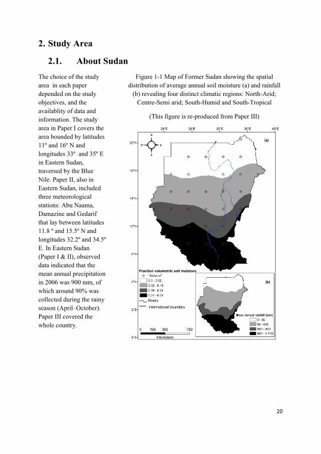
'^)^ m�� ��� ��� �The choice of the study area in each paper depended on the study objectives, and the availablity of data and information. The study area in Paper I covers the area bounded by latitudes 11º and 16º N and longitudes 33º and 35º E in Eastern Sudan, traversed by the Blue Nile. Paper II, also in Eastern Sudan, included three meteorological stations: Abu Naama, Damazine and Gedarif that lay between latitudes 11.8 º and 15.5º N and longitudes 32.2º and 34.5º E. In Eastern Sudan (Paper I & II), observed data indicated that the mean annual precipitation in 2006 was 900 mm, of which around 90% was collected during the rainy season (April–October).Paper III covered the whole country.

Figure 1-1 Map of Former Sudan showing the spatial distribution of average annual soil moisture (a) and rainfall

(b) revealing four distinct climatic regions: North-Arid; Centre-Semi arid; South-Humid and South-Tropical

(This figure is re-produced from Paper III)

21

{������� The Former Sudan (Fig. 1-1)1, was the largest country in Africa with an area of about 2.5 million km2. It extends over 17 lines of latitude from the Sahara region in North Africa to the Equator and 19 longitudes from the Congo basin in central Africa to the west, to the Red Sea in the East. The latest 5th Sudan Census of 2008 estimated the country’s population at about 39.5 millions (United Nations Population Fund [UNFPA], 2008). The climate ranges from arid in the north to tropical wet-and-dry in the far southwest. About two-thirds of Sudan lies in the dry and semi-dry region. There are major contrasts in rainfall (P) and potential evapotranspiration (PET), thus producing distinct climatic zones ranging within arid (North); semi arid (Centre); humid (South) and tropical (South), as classified using P/PET ratio (United nations Environmental Programme [UNEP], 1992; Hare and Ogallo, 1993). Sudan is drained mainly by the Nile River and its two main tributaries, the Blue and the White Nile. The Nile River is the longest river in the world, flowing for 6,737 km from its farthest headwaters in central Africa to the Mediterranean and is the lifeline for Sudan.

��������� the most significant climatic variables are rainfall and the length of the rainy season. From January to March, the country is under the influence of the dry northeasterly winds, and during this period there is almost no rainfall countrywide except for a small area in north eastern Sudan where the winds pass over the Mediterranean bringing occasional light rains. By early April, the rainy season starts from southern Sudan as the moist south westerlies reach the region, and by August the southwesterly flows extend to the northern limits. The dry northeasterlies begin to strengthen in September and to push south and cover the entire country by the end of December. Rainfall is negligible in the North, whereas equatorial climatic conditions prevail in south with annual rainfall of more than 1015 mmyr-1.Rainfall amounts decrease from the south to the north and the dry season lasts between three months in the humid tropical south and nine months in Khartoum with the hottest months being July and August. Since the 1960’s, rainfall has declined considerably.

There are two areas of interest in Sudan’s climate (El Tahir, 1989). These are the Bahr El Ghazal Basin in the southwestern corner of the country and the coastal area that forms a small strip along the Red Sea in the north-eastern part. Bahr El Ghazal Basin is characterised by high rainfall levels, with a rainy season of eight months. Two processes dominate the hydrology of Bahr El Ghazal basin, namely rainfall and evapotranspiration, while all the other processes are negligible. The Red Sea area lies in North-Eastern Sudan. The prevalent climatic conditions are characterised by low precipitation and high evapotranspiration. The mountains and the sea distinguish the area from the rest of the country and they influence the micro-climate within the region. Two contrasting rainfall regimes exist within this region. The area to the west of the mountain ranges experiences maximum rainfall during the summer (July/August) brought about by the south westerly monsoon winds which originate from the gulf of Guinea, whereas the area to the east receives maximum rainfall during the winter brought about by the north east and south east winds blowing over the Red Sea.

1This thesis was written before the sessesion of South Sudan in July-09-2011, therefore we refer here to former Sudan meaning both the North and the South.

22

�������� ����Temperatures do not vary greatly with the season at any location compared with many regions of the world. Summer temperatures often exceed 43.3°C in the northern desert zones. Dust storms, known locally as haboob, frequently occur. High temperatures also prevail to the south throughout the central plains region, and the humidity is generally low. In the vicinity of Khartoum, the capital of Sudan, the average annual temperature is about 37.1°C. January is the coolest month (with mean minimum 15°C and mean maximum 30°C ). June is the hottest month (with mean minimum 38°C and mean maximum 42°C). In southern Sudan the average annual temperature is about 29.4°C.

������������������� Similar to rainfall and temperature, annual actual evapotranspiration varies between the different climatic zones. June-September have the highest values while November-February have the lowest values of evapotranspiration. When relating potential evapotranspiration and rainfall values it appears that the area suffers climatically from acute water deficit.

����� The country's soils can be divided geographically into three categories. These are the sandy soils of the northern and west central areas, the clay soils of the central region, and the laterite soils of the south. Less extensive and widely separated, but of major economic importance, is a fourth group consisting of alluvial soils found along the lower reaches of the White Nile and Blue Nile rivers, along the main Nile to Lake Nubia, in the delta of the Qash River in the Kassala area, and in the Baraka Delta in the area of Tawkar near the Red Sea. Agriculturally, the most important soils are the clays in central Sudan that extend from the East through central to south western Sudan. Known as cracking soils because of the practice of allowing them to dry out and crack during the dry months to restore their permeability, they are used in the areas of the Gezira Scheme in central Sudan (the largest user of the Nile waters), the Rahad Project, the New Halfa Scheme, the Suki Scheme, the White Nile and Blue Nile Pumps Schemes, and the Kenana Sugar Scheme for irrigated cultivation. East of the Blue Nile, large areas are used for mechanized rainfed crops. West of the White Nile, these soils are used by traditional cultivators to grow sorghum, sesame, peanuts, and (in the area around the Nuba Mountains) cotton. The southern part of the clay soil zone lies in the broad floodplain of the upper reaches of the White Nile and its tributaries. Subject to heavy rainfall during the rainy season, the floodplain proper is inundated for four to six months, and a large swampy area, the Sudd, is permanently flooded. Adjacent areas are flooded for one or two months. In general this area is poorly suited for crop production, but the grasses it supports during dry periods are used for grazing. The sandy soils in the semiarid areas support vegetation used for grazing. Livestock raising is a major activity, but a significant amount of crop cultivation, mainly of millet, also occurs. Peanuts and sesame are grown as cash crops. These sandy soils are the principal area from which gum arabic is obtained through tapping of Acacia senegal (known locally as hashab). The laterite soils underlie the extensive moist woodlands found in South Sudan. Crop production in these soils is scattered, and the soils, where cultivated, lose fertility relatively quickly; even the richer soils are usually returned to bush fallow within five years.

23

����������� Open acacia communities are found in hill valleys and catchment areas of inland and coastal plains with bushes and trees of Acacia tortilis, a. radiana, a. etbaica, Salavadora persica, and Maerua crassifolia. Annuals and ephemerals include Cenchrus spp, panicum, Euphorbia spp, aristida, etc. Plant cover is less than 40% in the whole country, a percentage that may increase up to 50% due to seasonal growth. It portrays different land use types including agriculture, forests and range areas. Different agriculture forms include small holdings, mechanized and river bank farming. The area exhibits high land cover variability. It includes for example the Ar Roseris power dam and its lake. There are a number of forests for example the Sunut forest reseve and Okalma forest reserve. The forest reserve is a natural forest composed of a mixture of trees, mainly different types of Acacias, Balanites aegyptiaca plus other species. There is a large variation of age groups from young new regeneration to large groups of forest stands. The forests are related to the surrounding societies providing diversified benefits from the trees and the land. Regeneration and forest development factors are evident. Mountains include the Red Sea Hills in the North East, the Jabal Marra in the west, the Ingasana Hills is the south East, and the Nuba Mountains in the South West. The mountains constitute a source of sheet floods. Other areas are abandoned fallow land formed following abandonment of agricultural cropping. There are also the seasonal Khors (a gully or a seasonal water course is locally known as khor), running in different directions. The khors are characterised by the presence of degraded areas, natural regeneration, human activities such as agriculture, pastoralism and small settlements, as well as human intervention to reclaim the vegetation.

���������� ���� ���� -���� ������ The Khor system can be observed on a wide range of spatial scales, and each unit offers different environmental conditions for plant growth. Because of these broad scale geomorphological and finer scale topographic variations, there is an uneven distribution of water in the landscape, and hence variation in soil moisture. The moisture gradient associated with topographical variations has a strong influence on plant distribution. The transect that represents the different units in the landscape may also be viewed as a gradient, due primarily to variations in soil depth and soil moisture, which co-vary from the desert pavements to khors. The distribution of the available water resources is governed by a system of these khors. It is along the sides and on the beds of these khors that trees are found, agriculture is practiced, and where hand dug wells that provide the main water supplies are found. Gully erosion stripes off the fertile clay soils from the degradational clay plain forming bad-lands known locally as “Kerib” (Mirghani, 2007). Although erosion in the centre of the gully is visually apparent, its effects are not always detectable in terms of changes in soil quality (Ward et al., 2001). This indicates how geomorphologically-apparent desertification (Nir and Klein, 1974; Rozin and Schick, 1996) and changes in soil nutrient content are not necessarily congruent. Nonetheless, a decline in soil nutrients is recorded as some of the most important soil variables, and thus is likely to significantly impact plant growth. Although the major erosion usually occurs in the centre of the gully in a strip that is only 5– 30m wide, most plant biomass and species diversity are well concentrated there (Ward and Olsvig-Whittaker, 1993). Moreover, the concentration of the water current in the central erosion gully necessarily reduces the water flow to the adjoining

24

sides of the valley during floods. As a consequence of this reduction in water availability, leaching of salts is reduced (Shalhevet and Bernstein, 1968; Dan et al., 1973; Dan and Yaalon, 1982; Dan and Koyumdjisky, 1987) and soil salinity increases on the sides of the valley. Thus, even in the soil that remains un-eroded, soil quality declines over time.

'^'^ {���������������������������������The White Nile and its tributaries Sobat River, Bahr el Arab, Bahr el Ghazal, Bahr el Zeraf, Lol, Yei, Jur, Tonj, and Naam rivers, originate from Lake Victoria and Lake Albert in Uganda and also from Ethiopia and it contributes about 28% of the total flow of the Nile River. The Blue Nile and its tributaries, including the Rahad and Dinder rivers, rise in the Ethiopian highlands and it contributes about 59% of the total flow of the Nile River. Upon their confluence at Khartoum, the White Nile and the Blue Nile form the Nile River. The Nile River is joined after that, still in Northern Sudan, by the Atbara River which also originates in the Ethiopian highlands and contributes about 13% of the total flow of the Nile River. The Atbara River is the last tributary to join the Nile which thereafter flows through Northern Sudan and Egypt before emptying into the Mediterranean Sea (Collins, 2002). Despite the high contribution of the Blue Nile, its peak flow is largely seasonal, concentrated mostly in the months of June through to September and it is laden with silt that it carries over from the Ethiopian highlands. On the other hand, the relatively smaller contribution of the White Nile is mostly steady throughout the year, and, it is almost silt-free thus providing for the critical water needs of Sudan and Egypt during the low flow period of the Blue Nile. In addition to the Nile water Sudan has vast groundwater resources. Indeed, a number of groundwater basins such as the Upper Nile Basin fall across the borders between the North and the South, largely fed and replenished by the White Nile and its tributaries. The Nubian sandstone aquifer is shared by Sudan, Libya, and Chad. However, technical knowledge and data about these aquifers are, at best, quite limited, and therefore this resource remains largely untapped.

The waters of the Nile are governed mainly by two agreements. The first is the 1959 Nile Waters Agreement which allocated 18.5 Billion Cubic Meters (BCM) to Sudan and 55.5 BCM to Egypt (Salman, 2010). Sudan’s average use has so far ranged between 14 and 16 BCM annually. This agreement created a sense of animosity by some of the other eight Nile riparians countries namely Ethiopia (where 86% of the Nile waters come from), Eritrea, Uganda, Kenya, Tanzania, Democratic Republic of Congo, Rwanda, and Burundi of their right to an equitable and reasonable utilization of the Nile waters. The second agreement is the “Wealth Sharing” Agreement which is part of the 2005 Comprehensive Peace Agreement (CPA) between North and South Sudan2. Although this agreement provided detailed

2 The deal signed on 9 January 2005, between the North and the South known as Comprehensive Peace Agreement (CPA) brought temporary peace to Sudan ending Africa’s longest running civil war. The deal consisted of several protocols and agreements that governed the relationship between the North and the South during a six-year transitional period which ended with the referendum on self-determination for the South (Sudan Open Archive, 2005) in January 2011, and which was followed by the official birth of the new Republic of South Sudan on 9-July-2011.

25

provisions on sharing and management of land and natural resources in areas such as, land sharing and management, sharing of the oil revenues, monetary policy, banking, currency, borrowing, etc, it sadly omitted any but brief mention of water resources. Moreover, the agreement did not make an explicit mention of the groundwaters shared between the North and the South of the Sudan.

The hydro-politics of the Nile Basin are facing yet again a new challenge. Following the declaration of a new country, the Republic of South Sudan in July-09-2011, the total number of the Nile Basin riparian countries rose to eleven. The new country has developmental plans that involve using water resources for the generation of hydro-power, irrigation, as well as for domestic, livestock and industrial uses. The water will be provided from either surface and/or underground waters shared with one or more of these countries.

At the backdrop of this complex geopolitical situation, this thesis is an authentic addition to key technical knowledge about this important but often ignored resource.

26

~^ ���������In order to achieve the objectives that are stated above, a number of methods have been used, developed and/or modified. The methods used are grouped into three categories: the remote sensing methods; the statistical and geostatistical methods and the modelling methods. The details of the methods are outlined below according to this classification.

~^)^�����������������������

� ���������������

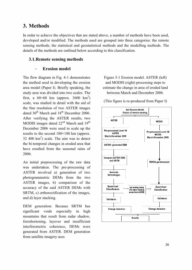
The flow diagram in Fig. 4-1 demonstrates the method used in developing the erosion area model (Paper I). Briefly speaking, the study area was divided into two scales. The first, a 60×60 km (approx. 3600 km2)scale, was studied in detail with the aid of the fine resolution of two ASTER images dated 30th March and 18th December 2006. After verifying the ASTER results, two MODIS images dated 22nd March and 19th

December 2006 were used to scale up the results to the second 180×180 km (approx. 32 400 km2) scale. The aim was to detect the bi-temporal changes in eroded area that have resulted from the seasonal rains of 2006.

An initial preprocessing of the raw data was undertaken. The pre-processing of ASTER involved a) generation of two photogrammetric DEMs from the two ASTER images, b) comparison of the accuracy of the said ASTER DEMs with SRTM, c) orthorectification of the images, and d) layer stacking.

DEM generation: Because SRTM has significant voids especially in high mountains that result from radar shadow, foreshortening, layover and insufficient interferometric coherence, DEMs were generated from ASTER. DEM generation from satellite imagery uses

Figure 3-1 Erosion model. ASTER (left) and MODIS (right) processing steps to

estimate the change in area of eroded land between March and December 2006.

(This figure is re-produced from Paper I)

27

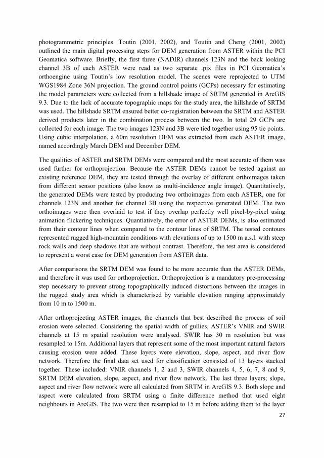
photogrammetric principles. Toutin (2001, 2002), and Toutin and Cheng (2001, 2002) outlined the main digital processing steps for DEM generation from ASTER within the PCI Geomatica software. Briefly, the first three (NADIR) channels 123N and the back looking channel 3B of each ASTER were read as two separate .pix files in PCI Geomatica’s orthoengine using Toutin’s low resolution model. The scenes were reprojected to UTM WGS1984 Zone 36N projection. The ground control points (GCPs) necessary for estimating the model parameters were collected from a hillshade image of SRTM generated in ArcGIS 9.3. Due to the lack of accurate topographic maps for the study area, the hillshade of SRTM was used. The hillshade SRTM ensured better co-registration between the SRTM and ASTER derived products later in the combination process between the two. In total 29 GCPs are collected for each image. The two images 123N and 3B were tied together using 95 tie points. Using cubic interpolation, a 60m resolution DEM was extracted from each ASTER image, named accordingly March DEM and December DEM.

The qualities of ASTER and SRTM DEMs were compared and the most accurate of them was used further for orthoprojection. Because the ASTER DEMs cannot be tested against an existing reference DEM, they are tested through the overlay of different orthoimages taken from different sensor positions (also know as multi-incidence angle image). Quantitatively, the generated DEMs were tested by producing two orthoimages from each ASTER, one for channels 123N and another for channel 3B using the respective generated DEM. The two orthoimages were then overlaid to test if they overlap perfectly well pixel-by-pixel using animation flickering techniques. Quantiatively, the error of ASTER DEMs, is also estimated from their contour lines when compared to the contour lines of SRTM. The tested contours represented rugged high-mountain conditions with elevations of up to 1500 m a.s.l. with steep rock walls and deep shadows that are without contrast. Therefore, the test area is considered to represent a worst case for DEM generation from ASTER data.

After comparisons the SRTM DEM was found to be more accurate than the ASTER DEMs, and therefore it was used for orthoprojection. Orthoprojection is a mandatory pre-processing step necessary to prevent strong topographically induced distortions between the images in the rugged study area which is characterised by variable elevation ranging approximately from 10 m to 1500 m.

After orthoprojecting ASTER images, the channels that best described the process of soil erosion were selected. Considering the spatial width of gullies, ASTER’s VNIR and SWIR channels at 15 m spatial resolution were analysed. SWIR has 30 m resolution but was resampled to 15m. Additional layers that represent some of the most important natural factors causing erosion were added. These layers were elevation, slope, aspect, and river flow network. Therefore the final data set used for classification consisted of 13 layers stacked together. These included: VNIR channels 1, 2 and 3, SWIR channels 4, 5, 6, 7, 8 and 9, SRTM DEM elevation, slope, aspect, and river flow network. The last three layers; slope, aspect and river flow network were all calculated from SRTM in ArcGIS 9.3. Both slope and aspect were calculated from SRTM using a finite difference method that used eight neighbours in ArcGIS. The two were then resampled to 15 m before adding them to the layer

28

stack. The river flow network was estimated using the hydrologic analysis package in ArcGIS9.3. When working with raster DEMs and computing slopes between grid cells, the ratio of the vertical and horizontal resolutions determines the minimum non-zero slope that can be resolved. In this study, the vertical resolution of the DEM was 1 m and the grid size was 15 m. Therefore the resolvable slope was calculated as 1/15=0.07. This value means that slopes on hillsides can be computed with a relatively small error. However, slopes in channels were often much smaller than this value. As a consequence, these areas appeared horizontal in the DEM. Therefore in order to avoid this problem, ArcGIS 9.3 uses an eight direction (D8) flow model. The direction of flow was determined by finding the direction of steepest descent, or maximum drop, from each cell. This was calculated as maximum drop = change in z-value/distance. The distance was calculated between cell centres. There are eight valid output directions relating to the eight adjacent cells into which flow could travel. One challenge arises if all neighbours are higher than the processing cell. In such a case the processing cell is called a sink and has an undefined flow direction because any water that flows into a sink cannot flow out. To obtain an accurate representation of flow direction across a surface, the sinks should be filled. The minimum elevation value surrounding the sink identifies the height necessary to fill the sink so the water can pass through the cell. A digital elevation model free of sinks is called depressionless DEM. Using the depressionless DEM as an input to the flow direction process, the direction in which water would flow out of each cell was determined. After determining the flow direction, then the flow accumulation was determined. Afterwards, a stream network was created by applying a threshold value to select cells with high accumulated flow in order delineate the stream network. More details on the technique of deriving flow direction from a DEM and on how to create river network in ArcGIS can be found in Jenson and Domingue (1988) and in Tang and Liu (2008).

After successful pre-processing the resulting orthorectified images were analysed. The image analysis involved supervised maximum likelihood classification aided by the authors’ knowledge of the area. Each image was trained into four land cover types: Gully, Flat land,Mountain and Water. Water bodies were clear and easy to train considering the fine ASTER resolution for both periods of the year. Mountains were also easily classified with the aid of the DEM. However, the most challenging task was to separate between Gully and Flat land since these two classes are bound to overlap and overlapping training area boundaries reduces the reliability of the training sites. To avoid this kind of overlap, a number of steps were taken. These steps included using MODIS vegetation indices (VI) as auxiliary data to discriminate between training classes. At first MODIS NDVI and EVI signatures are used to discriminate between stable and unstable vegetation. The unstable vegetation was seasonal and grew during the rainy season. That vegetation was flushed away with erosion, indicating that areas where there was unstable vegetation there was also erosion. The stable vegetation on the other hand was there throughout the year hence no erosion occurred. Where NDVI and EVI values are low, this is an indication of limited, unstable vegetation hence higher erosion risk. By contrast high values of NDVI and EVI indicated more stable vegetation. A second means of discriminate between Gullies and Flat land was by superimposing river network layer on top of the image to help guide the classification process. Other measures for ensuring

29

accurate classification included selecting bands that have better display, in either greyscale or as false colour composites FCC. Additionally, the classes are refined by varying the number of training areas until better accuracy is achieved. Better accuracies were also obtained through training as many areas as possible. Once the training areas are defined, then the signature separability values were studied. Signature separability is the statistical difference between pairs of spectral signatures. It is expressed in terms of Bhattacharrya Distance and Transformed Divergence. These are measures of the separability of a pair of probability distributions. Both Bhattacharrya Distance and Transformed Divergence are shown as real values between zero and 2. Zero indicates complete overlap between the signatures of any two classes while 2 indicates a complete separation between the two classes. The higher the separability value (i.e. more than 1.5) the more accurate the classification accuracy. The training areas are tuned until higher signature separability value of 1.5 or more are achieved. After achieving the best accuracies, the signature statistics report was studied in order to determine which channels of the 13 stacked layers were more significant in delineating erosion gullies.

Post classification steps were:

a) ASTER classification is validated via running an automatic random accuracy assessment analysis. This analysis was designed and implemented by generating a random sample of 300 points and comparing them to the original ASTER image. Each of the 300 samples was assigned to the different classes.

b) The area represented by each of the four classes is calculated using the function Generate Area Report in PCI Geomatica. Areas in the December image are subsequently subtracted from their correspondent areas in the March image in order to calculate the changed area per class.

Once ASTER classification results were accepted, the results were then up-scaled using MODIS. Upscaling was carried out by using the same training areas from ASTER, which were converted to shape files and superimposed on the MODIS products to guide the classfication of the latter. In this way the results of the of ASTER classification were generalized to larger areas covering the whole of the Blue Nile region. MODIS images were first georefrenced before undertaking a supervised classification using the same land cover classes and training areas as ASTER. Additionally, the classification was aided by using MODIS NDVI and EVI and river flow network layers as auxiliary data to discriminate between training classes. The outcome of MODIS classification was validated against field data using digital photos with co-ordinates and time taken in January 2007 from different locations. Finally the seasonal change in erosion area for the whole Blue Nile region was estimated.

30

� ��|m��������

SEBAL (Waters et al. 2002) is an instantaneous, i.e., time is constant, energy balance model. It considers the fact that evapotranspiration consumes energy and accordingly evapotranspiration ( AE ) is calculated as a residual of the energy balance (Eq. 1)

ss HGRλAE n ���� (1)

Where λAE is the instantaneous latent heat flux representing the energy available for evapotranspiration; nR is the net radiation; sG is soil heat flux, i.e., rate of heat storage into the soil and vegetation due to conduction; and sH is the sensible heat of flux. All the components have the units of ( -2mW � ).

In the SEBAL model, the net radiation is computed from spatially variable reflectance and emittance of radiation. The calculation requires spectral radiances in the visible, near infrared and thermal infrared regions of the spectrum to determine the intermediate parameters, such as surface albedo, NDVI and surface temperature. The soil heat flux, sG is computed as an empirical fraction of the net radiation using surface temperature, surface albedo and NDVI as input variables. The estimation of sensible heat flux, sH requires an iterative solution until sHconverges to the local non-neutral buoyancy for each pixel. The original MOD-1B level 1 versions 4 and 5 daily calibrated radiance with spatial resolution of 1 km and 36 bands for the year 2006 (available from http://ladsweb.nascom.nasa.gov/data/search.html) was used. Fourteen MODIS images dating from 07-January through 20-December 2006 were used. Each month was represented by minimum one image. MODIS’s NDVI is chlorophyll sensitive and it demonstrates a good dynamic range and sensitivity for monitoring and assessing spatial and temporal variations in vegetation amount and condition (Huete et al. 2002). It is successful as a vegetation measure in that it is sufficiently stable to permit meaningful comparisons of seasonal and inter-annual changes in vegetation growth and activity. In this study, the DEM is used to calculate the land surface albedo, emissivity, surface temperature over the horizontal plain of the image, and the surface roughness. These parameters are needed to solve Eq. 1 above. Together with land surface temperature and albedo, NDVI is used to calculate the leaf area index (LAI). LAI, in turn, is used to calculate Local surface roughness index (Z0m) for short grass or crop vegetation. Ultimately the Zero plane displacement height (d) is calculated. [Z0m] and [d] values are directly available from NASA’s table of Mapped Monthly Vegetation Data at

http://ldas.gsfc.nasa.gov/nldas/NLDASmapveg.php. Briefly speaking, the remote sensing procedure involved georefrencing and bands selection of MODIS data; mosacing and subsetting of the different images to fit the study area; preliminary analysis using false colour composites (FCC), instantaneous energy calculation using SEBAL model using Eq. 1 above and daily energy calculation using SEBAL model. The detailed calculation procedure of SEBAL model is available, among others, from Bastiaanssen et al. (1998a; 1998b; 2000; 2002; 2003), Mohamed et al. (2004), and Bashir et al. (2007a; 2007b).

~^'^���������������������������������������

� ��������� ��������������

Before undergoing trend analysis, the serial correlation of the data was studied, because the presence of serial correlation would affect the detection of trends in a series (Serrano et al.,

31

1999; Yue et al., 2002). The analysis for checking serial correlation is conducted by examining the lag-1 serial correlation coefficient (designated by r1) of the time series, which is calculated using the equation (2) by Haan (2002):

�

�

�

�

��

��

���

�n

tt

n

ttt

XXn

XXXXn

r

1

2

1

11

1

)(1

1

))((1

1

(2)

��

�n

tt nXX

1

� � � � � � � � � � (3)�

Where n is the sample size and 1 is the time lag.

The critical value for a given significance level, � is calculated by:

kn

knzqp

�

����� � 11

/ 2/1 � (4)

Where p and q are the upper and lower limits, respectively. �z is the critical value of the standard normal distribution for a given significant level � (5% in this case). If the calculated

1r was not significant at the 5% level, then the trend test was applied to original values of the time series. If, however, the calculated 1r was significant, prior to application of the test, the “de-seasoning” of the time series was obtained as (Partal and Kahya 2006; Luo et al., 2008;Chu et al., 2010):

11213112 ,,, ����� nn xrxxrxxrx � (5)

� ���������������

The Mann-Kendall trend test (Mann, 1945; Kendall, 1975) is regarded as a powerful tool for exploring trends in hydrological series. It is the most widely applied non-parametric test for detecting a trend in the hydro-meteorological variables with respect to climate change or variability (Abdul Aziz et al., 2006; Chen et al., 2007). Parametric and non-parametric methods have been extensively applied for detection of trends. Parametric tests are more powerful than the non-parametric tests, but there is an implicit assumption of normality of data that is seldom satisfied. Hydro-meteorological time series like SM are often characterized by data that are not normally distributed, and therefore nonparametric tests are considered more robust compared to their parametric counterparts (Hess et al., 2001). The Mann-Kendall test is distribution-free and therefore no assumption regarding the distribution of data is needed. A major advantage of this test is that it allows for missing data and can tolerate outliers. Mann Kendall test is a rank based approach that consists of comparing each value of the time series with the remaining in a sequential order.

The statistic S is the sum of all the counting as given in equation (6) below;

� ��

� ��

��1

1 1

n

k

n

kjkj XXSgnS (6)

32

Where

(7)

and Xj and Xk are the sequential data values; n is the length of the data set. A positive value of S indicates an upward trend and a negative value indicates a downward trend. The standardized test statistic (Zmk) is calculated by

(8)

Where the value of Zmk is the Mann- Kendall test statistics that follows standard normal distribution with mean of zero and variance of one. Thus, in a two sided test for trend, the null hypothesis of no trend, Ho cannot be rejected if

(9)

Where α is the significance level that indicates the strength of the trend. In the present study, significance level of 5% was applied.

� �������������������

The relationships between soil moisture and rainfall and temperature inherently vary over space, and can be analyzed using geographically weighted regression (GWR) technique. GWR, a recent refinement of ordinary linear regression models, is a local spatial statistical technique used to analyse spatial non-stationarity when the measurement of relationships between variables differs from location to location. First the relationship was explored using the following equation of the ordinary least square regression (OLS) below:

������ RainfalleTemperatur 210 BBBSM (10)

In this model, the dependent variable was mean monthly soil moisture (mm), the two independent variables were mean monthly temperature (°C), and average monthly rainfall (mm). B0, B1 and B2 regression coefficients, and ε is the residual. This model assumed spatial stationarity in the relationship among the different variables under study.

In comparison to the OLS, the GWR base equation used in the multivariate regression analysis is:

),(Rainfall),(eTemperatur),(),(),( 210 vuvuBvuBvuBvuSM ������ (11)

33

Where (u,v) are the location coordinates of a particular point on a surface.

This method takes into consideration the local variations in rates of change with resulting coefficients calculated by the model that are specific to each location (Brundson et al., 1996). Therefore, it has emerged as one of the more effective methods to account for, and to examine the presence of spatial non-stationarity in relationships (Fotheringham et al., 1998). In particular, the parameter estimates are calculated by using a weighting method in which the contribution of an observational site to the analysis is weighted in accordance with its spatial proximity to the specific location being considered. Thus, the weighting of an observation in the analysis is not constant but a function of its location. Observations close to the centre of the window are weighted more heavily than observations further away. The derived parameters can then be mapped to identify the nature of their variation in space and thus bring out the spatially varying relationships among the different variables. In this method, parameter estimation is highly dependent on the weighting function and kernel used.

NDVI data were used as weight variables in the analysis. The GWR analysis was conducted using an adaptive kernel method. A small bandwidth results in very rapid distance decay, while a large value results in a smoother weighting scheme. The variable bandwidth approach was chosen and optimized by cross-validation minimisation to account for the spatial variation in the size of the different climatic regions, and hence the density of these regions’ centroids.

� m������+������m+�������������������% ���������

To further understand dry and wet variations in terms of regeneration demand, the aridity index is calculated in this study (Paper III). Aridity index, AI , as defined by de Martonne (1926) who used it to study irrigation demands (Zhang et al., 2009) is computed as: �

10

12

��

TP

AI (12)

Where P is the monthly precipitation amount; T is the monthly mean air temperature.

The aridity index aims to identify the months when irrigation is necessary. Generally, irrigation is necessary when AI <20.�

~^~^������������������

� ��������������������x�����������|�������������

The Thornthwaite water balance model (Thornthwaite and Mather 1955) is usually applied with monthly or daily rainfall time step. The use of daily values is preferred over monthly values when possible, particularly in dry locations, where precipitation only occurs occasionally except in the rainy season. In such a case monthly totals cannot reflect the dynamics of soil moisture. In this study, the water balance calculations are performed on a daily time step. There are different variants of the Thornthwaite water balance model, and the basic procedure of the model used in this study is similar to that used by Xu and Chen (2005).

The soil moisture storage is computed as:

34

tAEtP1tWtW ���� (13)Where tW is the current soil moisture, 1�tW is the soil moisture in the previous time step, Pt is precipitation, and AE t is actual evapotranspiration at time step t.

� If potential evapotranspiration PEt ≤ Pt, then AE t = PEt. Wt is first estimated with surplus (runoff and/or recharge) = 0. When Wt > FC (field capacity), surplus = Wt – FC, and Wt is set to FC;

When Wt ≤ FC, Surplus =0.

� If PEt > Pt, soil water will be depleted to compensate for the supply. At the same time, one has AE t < PEt and surplus = 0. Under this condition, AE t is calculated using equation (14) below

FC1tW

tPEtAE ��� (14)

In this study two modifications are made. In the original model the potential evapotranspiration, PEt is calculated using the temperature based Thornthwaite equation, which is an empirical and site-specific estimation. In this study it is calculated using the Penman- Monteith equation which is a physically based model that proved to be more reliable in various parts of the world (Allen et al. 1998). The second modification is towards the calculation of actual evapotranspiration using equation (14). In arid climates, especially during the dry and transit seasons, soil moisture is generally very low, and as a consequence, the value of Wt-1/FC can be very small (nearly zero). Equation (14) may therefore significantly underestimate actual evapotranspiration especially in a dry season with occasional small rain. To overcome this drawback, actual evapotranspiration was calculated using a modified equation (14a).

� �

��� ����

FC1tW

tPEtP ,tPEmintAE (14a)

In practice, if the initial soil moisture is unknown, which is typically the case, a balancing routine is used to force the net change in soil moisture from the beginning to the end of a specified balancing period (N time steps) to zero. To do this, the initial soil moisture is set to the water-holding capacity and budget calculations are made up to the time period (N+1). The initial soil moisture (W1) at time 1 is then set to be equal to the soil moisture at time N+1 and the budget is re-computed until the difference W1 – WN+1 reduces to a certain value that is less than a specified tolerance.�

One of the parameters that has to be specified is the field capacity (FC) of soil. FC is also known as the soil water holding capacity. It represents the amount of water remaining in the soil after the soil layer has been saturated and the free or drainable water has been allowed to drain away, i.e. after a few days of substantial rain event(s). The soil water holding capacities in the study region are approximately 205, 108, and 154 mm in 1 meter deep soil for stations Abu Naama, Damazine and Gedarif, respectively (available from National oceanographic and atmospheric administration NOAA). In this study this method is used as a reference method, because it is based on the water balance calculation.

35

� �������������������������������������

Based on energy balance, Bouchet (1963) derived the complementary relationship between actual and potential evapotranspiration; it states that as the surface dries the decrease in actual evapotranspiration is accompanied by an equal, but opposite, change in the potential evapotranspiration. This relationship is described as:

AE + PE = 2 ETW (15)

Where AE , PE and ETW are actual, potential and wet environment evapotranspiration, respectively. The complementary relationship has formed the basis for the development of several evapotranspiration models (Morton 1983; Brutsaert and Stricker 1979; Granger and Gray 1989), which differ in the calculation of PE and ETW. AE is usually calculated as a residual of (Eq. 1). Complementary relationship calculation methods are now increasingly used to calculate actual evapotranspiration because they require only observations on climate variables and bypass complex and poorly understood soil-plant processes (Xu and Singh 2005). Previous studies (Xu and Chen 2005) showed that the model developed by Granger and Gray (1989) is a good choice.

Considering the general case of evapotranspiration from an unsaturated surface at some rate less than the potential, i.e., 0 < AE < PE , Grange and Gray (1989) defined relative evapotranspiration, the ratio of actual to potential evapotranspiration, G = AE / PE , as aunique parameter for each set of atmospheric and surface conditions. In other words, the surface conditions play a predominant role in the partitioning of the energy available for evapotranspiration, and thus also control potential evapotranspiration. For a wet surface, G will be equal to unity; while for a very dry surface, G will approach zero. Based on the above consideration, Grange and Gray (1989) modified Penman’s (1948) energy balance equation for calculating potential evapotranspiration into equation (16) to calculate the actual evapotranspiration:

aEγΔG

γGλ

nR

γΔG

ΔGAE

��

�� � (16)�

where nR is the net radiation near the surface, � is the latent heat, � is the slope of the saturation vapour pressure curve at the air temperature, � is the psychometric constant, and Ea is the drying power calculated as follows:

))(( asza eeUfE �� (17) Where f (Uz) is some function of the mean wind speed at a reference level z above the ground; and ea and es are the actual vapour pressure of the air and the saturation vapour pressure at the air temperature, respectively. Penman (1948) originally suggested an empirical linear approximation for f (Uz) which is used here:

)54.01(0026.0)( 22 UUf �� (18) Granger and Gray (1989) further derived that the relative evaporation G can be calculated as:

DeG

045.8028.01

1

�� (19)

36

Where )//( �naa REED �� is the relative drying power. Granger (1998) modified equation (19) to

De

GD

006.02.0793.0

1902.4

��

� (20)

Previous studies (Xu and Chen, 2005; Xu and Singh 2005) showed that the constants 0.793 and 0.2 in equation (20) need to be locally calibrated to improve the estimation by the GG method, and suggested a general form as

Deba

GD

006.01

902.422

��

�(21)

Where a2 and b2 are considered as parameters to be calibrated.

In order to calibrate parameters a2 and b2 to give the best estimate of actual evapotranspiration using equation (16), the total annual actual evapotranspiration data is needed, which is not available in the study region. Annual evapotranspiration is thus calculated based on the Budyko-type framework as a function of the aridity index. Different empirical equations of this type exist (e.g., Dooge, 1992; Xu and Singh, 2004) to describe this relationship (i.e., Schreiber 1904; Ol’dekop 1911; and Pike 1964), which are expressed, respectively, as

)]exp(1[P

PE

PE

P

PE

AE��� (22)

)tanh(PE

P

PE

AE� (23)

2)(1/PE

P

PE

P

PE

AE�� (24)

Where AE , P and PE are the annual actual evapotranspiration, precipitation, and potential evapotranspiration as calculated by Penman-Monteith equation (Allen et al. 1998) respectively. In this study the average value calculated by these three methods is used as the annual total actual evapotranspiration for calibrating parameters a2 and b2 in the GG method.�

�

37

�^ ��� �������� ��� �������^)^&����� +�� #������������� ���� �������� �������� ��� ������ ��� ��� ����

�����������������������������������������������������������

m����� �������������������������������������

Two DEMs were extracted from the two ASTER images and were compared to SRTM. The results (Figure 4a and 4b, Paper I) showed that the two ASTER-generated DEMs suffered vertical errors and were less accurate than SRTM. One reason can be the fact that the study area is predominantly a rural area with few land cover/use classes, therefore it is characterised by low optical and radiometric image contrast. Also the accuracy of the ground control points (GCPs) was among the main factors limiting the accuracy of ASTER DEM (Table 2, Paper I). Compared to the SRTM, ASTER DEM systematically overestimated elevation at higher latitudes while it underestimated elevation at low altitudes (Figure 5, Paper I). The maximum errors occurred at sharp ridges or deep gullies. Accordingly SRTM was used as the DEM source in this study.

�����������������������������������������������������������������

The bi-temporal two scale soil erosion model which was developed in the study, was used to map the spatial distribution of gully erosion in the Blue Nile region during 2006 seasonal rains. A regional spatial distribution map of seasonal gullies in the Blue Nile was produced (Fig. 5-1). It is seen in the figure that gully erosion is evident in and around the Blue Nile River and its tributaries. The bi-temporal classification of ASTER images resulted in an estimation of the increase in the area of gullies. The increase is estimated at approximately 112 km2 (8.7%) of the total image area (Table 7, Paper I) during the rainy season of 2006. The classification of MODIS products allowed the identification and estimation of erosion on a regional scale. During the same period, erosion was estimated at 2071 km2 (6.5%) of the total MODIS area (Table 8, Paper I). The classification of ASTER March was better than ASTER December because VNIR and SWIR channels are more capable of discriminating erosion gullies in the dry season that is characterised by less soil moisture and therefore has higher spectral reflectance. The overall accuracy of MODIS is less than that of ASTER because there is insufficient spectral distinctiveness due to the low spectral and spatial resolution of the MODIS data. Also MODIS products consist of averaged products rather than the actual spectral bands. There were some artefacts in MODIS that interfered with the calculation of eroded areas. The results of this study should be viewed in light of the facts that: (a) the year 2006 was an exceptionally wet year compared to previous years, (b) the Upper Blue Nile River is steeper and receives more rain than any other rivers in Sudan namely, the White Nile, River Atbara, Sobat, etc., and (c) there has not been any similar previous studies reported in this region.

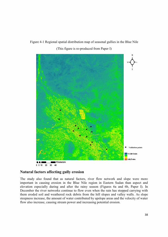
38

Figure 4-1 Regional spatial distribution map of seasonal gullies in the Blue Nile

(This figure is re-produced from Paper I)

������������������

"�� ����������������������� ������������

The study also found that as natural factors, river flow network and slope were more important in causing erosion in the Blue Nile region in Eastern Sudan than aspect and elevation especially during and after the rainy season (Figures 6a and 6b, Paper I). In December the river networks continue to flow even when the rain has stopped carrying with them eroded soil and weathered rock debris from the hill slopes and valley walls. As slope steepness increase, the amount of water contributed by upslope areas and the velocity of water flow also increase, causing stream power and increasing potential erosion.

39

�^'^&����� ++�� ������ �������� ���� ����������� ��� ����������������������������

�������������������������������� �������������������������Comparisons of the daily AE (Figure 3, Paper II) and monthly AE (Figures 7a-7c, Paper II) estimates revealed that in the dry season (November – April) and the transit season from dry to wet (May – June), the AE calculated by the SEBAL and GG methods were significantly higher than those by the WB method. This is because during the dry season the soil moisture is very low, hence lowering the WB estimate of AE . The other two methods failed to catch this reality and hence they overestimated AE . In the wet season (July-October), there is generally better agreement between the SEBAL method and the WB method than that between the GG method and the WB method, although this agreement varied for particular days and stations (Figure 5, Paper II). The GG method showed an underestimation of daily AE in the wet season. Generally speaking there was better correlation between SEBAL and WB than between GG and WB estimates. The estimated daily AE followed the trend of soil moisture variation whereas the seasonal pattern of AE was a result of the combined effect of rainfall and soil moisture.

����������� ���������������������� �������|m��

Subsequently, SEBAL was used to map actual evapotranspiration in the region (Figure 5-2: a-l). The figure revealed that during the dry period (j, k, l, a, b, c, and d) the north-east of the Blue Nile exhibits low levels of AE which is approximately 0-20 mm month-1, because this region is bare land and very dry at this time of the year. During the same period, the southern region which is between the Blue and the White Nile rivers showed higher rates of AE as indicated by the yellow/green colour correspondent to AE ≈ 30-90 mm month -1. The highest evapotranspiration rates were found in north-western region between the White and the Blue Niles where the Gezira scheme is located which resulted from the irrigation activities. However, during the wet period (e, f, g, h, and i), and without the influence of irrigation activities, a different picture was found. The highest AE values ( AE ≈ 90-150 mm month -1)were found in the south-east part of the study region, and were decreasing towards the north-west. This was a reflection of the spatial distribution of rainfall in the study region. The rainfall pattern is such that the south-eastern area has more rain during the rainy season than the north-western area (El Tom, 1975). The spatial distribution of AE was a combined result of the amount of rainfall and the availability of soil moisture, which played different roles in different seasons. In conclusion, the spatial distribution maps of monthly AE produced by the SEBAL method show that in the dry season, the spatial distribution pattern is determined by the location, aspect, land use and irrigation activities. During the wet season, the spatial distribution pattern of monthly AE follows that of the rainfall distribution.

�

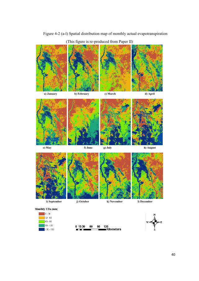
4�

Figure 4-2 (a-l) Spatial distribution map of monthly actual evapotranspiration

(This figure is re-produced from Paper II)

a) January b) February c) March d) April

e) May f) June g) July h) August

i) September j) October k) November l) December

41

�^~^&����� +++�� #������������� ��������� �������� ��� ���� ����� ����� ������������������������������ �� ��������������������� �������������� ��������������������������������^��

!� �� ��������������������������� ������"y�&������������)���������� ����In Sudan as was pointed out in Paper II, the soil moisture pattern follows that of the rainfall very closely. When rainfall increases, soil moisture also increases due to an increase in surface evapotranspiration without any significant change in the atmospheric moisture convergence (Douville et al., 2001). The soil-precipitation two-way interaction is commonly referred to as a positive feedback, since the water added to the land surface during a precipitation event leads to increased evapotranspiration, and this in turn can lead to further rainfall. In order to understand the nature of this soil moisture variability, not only in relation to rainfall, but also in relation to temperature changes, the Mann Kendall test was used.

m�� ������������During the period 1965-2005 soil moisture and rainfall decreased while temperature increased significantly using MK test at 95% confidence interval (Figure 3, Paper III). These trends are detected in the annual series as well as in wet season when the seasonal series was analysed (Figure 4, Paper III). These results are consistent with previous studies (e.g., Alvi, 1994; Janowiak, 1988; Nicholson et al., 2000). Changes in soil moisture are more dominated by changes in temperature than in rainfall. Although rainfall amounts decreased all over the country, only significant decline was noted in the south eastern parts as Osman and Shamseldin (2002) had pointed out also in their study. Generally higher month-to-month variability had characterized the temperatures, with significant increases in the northern and central parts. The observed change in temperature could be partly a consequence of local climatic and human forces, such as change in rainfall pattern (periodic drought), rapid increase in population and the mismanagement of land and water resources, desert encroachment and soil erosion, the interaction of which could modify the local climatic conditions (Hulme, 1989; Hulme and Kelly, 1993). The rainfall amounts decreased in all months (Figure 4, Paper III). In August, the rainfall decreased significantly (solid red inverted triangles) in the southern parts. Trilsbach and Hulme (1984) also reported that heavy rains in the rainy season declined more than median and light rains, and the steepest decline occured in August.

During the dry season the soil moisture continued to show significant decreasing trends in all months but the change was less dramatic or softer than the wet season (Figure 4, Paper III). January temperatures decreased significantly. This affected the western and southern parts of Sudan. February temperatures remained unchanged except for an increase in three stations in the South. March temperatures were a mixture of both decreasing (west) and increasing (south and east) significant trends. During December-March soil moisture continued to decrease despite the unchanged or the decreasing temperatures during the same period. This was attributed partly to other unconsidered factors and to a slight decrease in rainfall. Rainfall decreased in all months although not significantly.

In order to quantitatively evaluate the impact of the rainfall and temperature changes on the decline of soil moisture, the Geographically Weighted Regression (GWR) was used (Figure 5, Paper III). The GWR performed differently in different months and different regions in reflecting the relationship between SM, rainfall and temperature. The GWR performance was reflected by the local estimate of the coefficient (R2). In northern Sudan and because of the

42

shortages in rainfall, there is no evidence of correlation (R2 ranged between 0.0 to 0.3). During dry months, under the influence of dry north-easterlies, there is practically no rainfall countrywide except for a small area in north-eastern Sudan by the Red Sea. However, during the rainy season July, August, September and October, South Sudan also showed no correlation. The reason could be because of the heterogeneity across the south in terms of physical characteristics (soils, topography, and microclimate) that affect the relationships. For example the rainy season, which increases in length from north to south, has a great effect on the temperature regimes. During the rainy season, temperature drops significantly in the south, where the dry season is short, thus making the peak wet months cooler than the winter months (UNEP, 1992; Hare and Ogallo, 1993). Therefore the GWR relationship does not hold in such a case. In central Sudan, the temperature moderates during the wet season and hence central Sudan shows weak to strong correlations (R2 0.3-0.6 and above). During the rainy season this relationship is stronger. The SM predicted by the GWR both in time and space was compared to NCEP/NCAR SM data (Figure 5, Figure 6, Paper III). For the prediction of SM data in time, the data set of monthly time series is split into two. The data set for the period 1965-2004 was used for running the GWR model, and the data set of the year 2006 is used as a control for the verification of the model. The result indicated that the model predicted the SM well (R2 = 0.9). For predicting SM in space, the model was used to predict SM in Ad’Damazine station located in south eastern Sudan (at longitude 34.4° W and latitude 11.8° N). The model was fed with observed data of mean monthly rainfall and temperature from the year 2006. The relationship between predicted and “observed” data for Damazine was strong (R2 = 0.8). The ability of GWR to predict both in space and time makes it a strong competitor to traditional methods of regression analysis like Ordinary Least Square (OLS).

m�����������������������������% ����������Long-term average AI was calculated for the period 1965-2005. AI <20 is shown in yellow and AI> 20 is shown in green colour (Figure 5-3). This long-term AI was then compared to the average AI of the last 10 years, 1995-2005 with AI> 20 (shown as horizontal lines). During the dry season the AI is below 20 for all the country (except a smaller patch in the south) during both periods. There is therefore very little or no-change in the AI for the past 40 years because there is no rainfall during this season. During the wet season May, July and September the last ten years of the study period showed more areas with AI >20 (horizontal lines). This was attributed to increases in rainfall that were experienced since the mid nineties (Elagib and Mansell, 2000, Hulme et al., 2001). The long term AI>20 for the whole period (1965-2005) was lower probably because of the reported decline in rainfall especially in semi-arid central Sudan since 1965 and which continued and intensified in the 1980s, with 1984 the driest year on record (Walsh, et al., 1988 and Hulme, 1990). When compared to NDVI data, the aridity index AI, performed well in the wet season in reflecting the wet conditions in Sudan.

� �

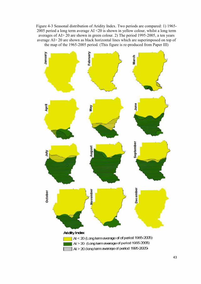
43

Figure 4-3 Seasonal distribution of Aridity Index. Two periods are compared: 1) 1965-2005 period a long term average AI <20 is shown in yellow colour, whilst a long term averages of AI> 20 are shown in green colour. 2) The period 1995-2005, a ten years

average AI> 20 are shown as black horizontal lines which are superimposed on top of the map of the 1965-2005 period. (This figure is re-produced from Paper III)

44

�

}^ y���� ������������������������The vegetation-soil moisture relationships describe the various vegetation patterns which occur in the country. These patterns occur on a variety of soils developed from different parent materials. Often the equilibrium between the vegetation and the environment is delicate and easily displaced due to climate change or interference of man, leading to the destruction of the pattern and the establishment of more xerophytic vegetation. Natural regeneration of Sudan’s vegetation remains the only possible solution for combating this degradation and ultimately contributing to the country economic and social stability. In light of these facts the current thesis tries to understand the physical circumstances that impact vegetation regeneration via studying the connections between soil water, erosion and some of the main elements of the hydrological cycle, namely evapotranspiration, temperature and rainfall. The studies of soil moisture and its climatic and degradation associations in Sudan are rare especially in the thorough way that is presented here. These results have important food security implications, informing agricultural development, environmental conservation, and water resource planning.

This research work addressed the problem of soil erosion and identified erosion gullies and subsequently estimated the eroded area. The research results identified river flow network and slope as more important natural factors, in causing erosion in the Blue Nile region than aspect and elevation. An evaluation of evapotranspiration as a direct reflection of the dynamics of soil moisture and hence vegetation regeneration resulted in the production of a sequence of spatial distribution maps of seasonal actual evapotranspiration. From the maps it was concluded that in the dry season, the spatial distribution pattern is determined by the location, aspect, land use and irrigation activities. In the wet season, the spatial distribution pattern followed that of the rainfall distribution. The seasonal pattern of actual evapotranspiration was a result of the combined effect of rainfall and soil moisture. The seasonal patterns of monthly soil moisture followed those of the monthly rainfall, but there was about one month delay in the phase with the peak of the monthly rainfall appearing in July for all three stations while the peak of the monthly soil moisture appearing in August/September.

An evaluation of the soil moisture, temperature and rainfall variability concluded that:

� There are decreasing trends of SM in Sudan on an annual and seasonal level and that this trend is less dramatic or weaker in the dry season (November-April) than the wet season (May-October).

� Soil moisture variability follows closely that of rainfall and temperature. The results also show that SM variability followed temperature changes more closely than rainfall.

� The spatio-temporal variability of the aridity index, AI, showed that the long-term average of AI is affected by the widely reported decline in rainfall during 1965-1985. The decadal AI average of 1995-2005 gave evidence of increases in rainfall that have been reported since the mid-nineties. During the wet season, the aridity index AI, performed well in reflecting the wet conditions in Sudan.

45

The evaluation procedure and results presented in this thesis provide valuable information and references for better understanding of soil moisture variation in Sudan and its implication for vegetation regeneration. We have made some exploration of how to assess the irrigation requirements under arid, semi-arid and semi-humid environments and the results could serve as an important index for a comprehensive appraisement of the ecosystem and for sustainable development.

�^ ������������� Abdul Aziz O.I. and Burn, D.H. (2006). Trends and variability in the hydrological regime

of the Mackenzie River Basin. Journal of Hydrology, v319, nr 1-4, pp 282–294� Allen, R. G., Pereira, L. S., Raes, D., and Smith, M. (1998). Crop evapotranspiration:

guidelines for computing crop water requirements, United Nations FAO, Irrigation and Drainage, Rome, Italy, 300p,

� Alvi, S.H. (1994). Climate changes, desertification and the Republic of Sudan. Geojournal, V33, nr. 4, pp 393-399.

� Ayoub, A. T. (1998). Extent, Severity and Causative Factors of Land Degradation in Sudan, Journal of Arid Environments, v38, pp 397–409.

� Bashir, M. A., Hata, T., Tada, A., Tanakamaru, H., and Abdelhadi, WA. (2007a). Estimating actual evapotranspiration using surface energy balance algorithm for land, SEBAL for Gezira scheme. Part I: Determination and calculation of intermediate parameters. Sudan Journal of Agricultural Research, v8, pp 65–76.

� Bashir, M.A., Hata, T., Tada, A., Tanakamaru, H., and Abdelhadi, W. A. (2007b). Estimating actual evapotranspiration using surface energy balance algorithm for land, SEBAL for Gezira scheme. Part II: Application and validation. Sudan Journal of Agricultural Research, v8, pp 77–87.

� Bastiaanssen, W. G. M. (2000). SEBAL-based sensible and latent heat fluxes in the irrigated Gediz Basin, Turkey. Journal of Hydrology, v229, nr 1-2, pp 87–100.

� Bastiaanssen, W. G. M., Ahmed, M., and Chemin, Y. (2002). Satellite surveillance of evaporative depletion across the Indus Basin. Water Resources Research, v38, nr 12, pp 1273–1282.

� Bastiaanssen, W. G. M., and Chandrapala, L. (2003). Water balance variability across Sri Lanka for assessing agricultural and environmental water use. Agriculture and Water Management, v58, nr 2, pp 171–192.

� Bastiaanssen, W. G. M., et al. (1998b). The surface energy balance algorithm for land, SEBAL. Part 2. Validation. Journal of Hydrology, 212/213, pp 213–229.

� Bastiaanssen, W. G. M., Menenti, M., Feddes, R. A., and Holtslag, A. A. M. (1998a). The surface energy balance algorithm for land, SEBAL. Part 1. Formulation. Journal of Hydrology, 212/213, pp 198–212.

� Beniston M, Stephenson DB. (2004). Extreme climatic events and their evolution under changing climatic conditions. Global Planet Change v44, pp 1–9

� Bosilovich, M. (2008). NASA’s modern era retrospective analysis for research and applications: Integrating Earth observations. Earthzine, www.earthzine.org

� Bouchet, R. J. (1963). Evapotranspiration réelle et potentielle, signification climatique.” General Assembly Berkeley, Int. Assoc. Sci. Hydrol., Gentbrugge, Belgium, Publ. No. 62, pp 134–142.

46

� Brunsdon, C., Fotheringham, A.S. & Charlton, M.E. (1996). Geographically weighted regression - a method for exploring spatial nonstationarity. Geographical Analysis, v28, nr 4, pp 281-298

� Brutsaert W. (2006). Indications of increasing land surface evaporation during the second half of the 20th century. Geophysical Research Letters, v33, L20403

� Brutsaert, W., and Stricker, H. (1979). An advection-aridity approach to estimate actual regional evapotranspiration. Water Resources Research, v15, nr 2, pp 443–449.

� Butcher A D. (1938). The Sadd Hydraulics. Ministry of Public Works Cairo, Egypt � Cadet DL, Nnoli NO. (1987). Water vapour transport over Africa and the Atlantic Ocean

during summer 1979. Quart Journal of the Royal Meteorological Society, v 113, nr 476, pp 581–602

� Camberlin P. (1995). June–September rainfall in north-eastern Africa and atmospheric signals over the Tropics: a zonal perspective. International Journal of Climatology, v15, pp 773–783

� Chan S.-O, Eagleson P S. (1980). Water balance studies of the Bahr el Ghazal swamp Report No. 261, Department of Civil Engineering, Massachusetts Institute of Technology.

� Chen MY, Xie P, Janowiak JE, and Arkin PA (2002). Global Land Precipitation: A 50-yr Monthly Analysis Based on Gauge Observations. Journal of Hydrometeorology, v3, pp 249-266

� Chen Y, Li W, Xu C, Hao X. (2007). Effects of climate change on water resources in Tarim River Basin, Northwest China. Journal of Environmental Science, v19, nr 4, pp 488-493

� Chu, J.T., Xia, J., Xu, C-Y, Li, L., Wang, Z.G. (2010). Spatial and temporal variability of daily precipitation in Haihe River basin, 1958–2007. Journal of Geographical Sciences v20, nr 2, pp 248-260.

� Collins R. (2002). The Nile, Yale University Press. � Cook KH, Vizy EK. (2006). Coupled model simulations of the West African monsoon

system: twentieth and twenty first century simulations. Journal of Climate, v19, pp 3681–3703

� Courault, D., Seguin, B., and Olioso, A. (2005). Review on estimation of evapotranspiration from remote sensing data: From empirical to numerical modeling approaches. Irrigation and Drainage Systems, v19, nr 3–4, pp 223–249.

� Dan, J. and Koyumdjisky, H. (1987). Distribution of salinity in the soils of Israel. Journal of Earth Sciences, v36, pp 213–223.

� Dan, J. and Yaalon, D. H. (1982). Automorphic saline soils in Israel, in: Aridic soils and geomorphic processes, edited by: Yaalon, D. H., Cathena Verlag, 1, Braunschweig, Germany, pp 103–115.

� Dan, J., Moshe, R., and Alperovitch, N. (1973). The soils of Sede Zin, Israel. Journal of Earth Sciences, v22, pp 211–227.

� de Martonne E. (1926). Une nouvelle fanction climatologique: l’indice d’aridité. La Météorologie v2, pp 449–458

� Dooge, J. C. I. (1992). Hydrologic models and climate change. Journal of Geophysical Research, v97, nr D3, pp 2677–2686.

� Douville, H., Chauvin, F. and Broqua, H. (2001). Influence of Soil Moisture on the Asian and African Monsoons. Part I: Mean Monsoon and Daily Precipitation. Journal of Climate, v14, nr 11, pp 2381-2403

� El Tahir EAB. (1989). A Feedback Mechanism in Annual Rainfall in Central Sudan, Journal of Hydrology, v110, pp 323-334.

47

� El Tahir EAB. (1992). Drought frequency analysis of annual rainfall series in central and western Sudan. Journal of Hydrological Sciences, v 37, pp 185–199

� El Tom, M. A. (1975). The Rains of the Sudan: Mechanisms and Distribution, Khartoum University Press, Khartoum, Sudan.

� Elagib, Nadir A. and Mansell Martin G. 2000. Recent trends and anomalies in mean seasonal and annual temperatures over Sudan. Journal of Arid Environments, v45, nr 3,pp 263–288

� Fontaine B, Roucou P, Trzaska S. (2003). Atmospheric water cycle and moisture fluxes in the West African monsoon: mean annual cycles and relationship using NCEP/NCAR reanalysis. Geophysical Research Letters, v30, nr 3, pp 1117. doi:10.1029/2002GL015834

� Fotheringham, A.S., Brunsdon, C. & Charlton, M.E. (1998). Geographically weighted regression: a natural evolution of the expansion method for spatial data analysis. Environment and Planning A, v30, nr 11, pp1905-1927

� Gao, G., Chen, D. L., Xu, C-Y., and Simelton, E. (2007). Trend of estimated actual evapotranspiration over China during 1960-2002. Journal of Geophysical Research-Atmospheres, v112, D11120,10.1029/2006JD008010.

� Granger, R. J., and Gray, D. M. (1989). Evaporation from natural non saturated surfaces.” Journal of Hydrology, v111, nr 1-4, pp 21–29.

� Hann CT. (2002). Statistical methods in hydrology. Second version. Blackwell Publishing � Hare F. K. and L. A. J. Ogallo. (1993). Climate Variations, Drought and Desertification.

World Meteorological Organization, Nr. 653 � Hess, A., Iyer, H. & Malm, W. (2001). Linear trend analysis: A comparison of methods.

Atmospheric Environment, v35, nr 30, pp 5211-5222� Huete, A., Didan, K., Miura, T., and Rodriguez, E. (2002). Overview of the radiometric

and biophysical performance of the MODIS vegetation indices. Remote Sensing of Environment, v83, nr 1–2, pp 195–213.

� Hulme M, Tosdevin N. (1989). The Tropical easterly Jet and Sudan rainfall: a review. Theoretical and Applied Climatolology, v39, nr 4, pp 179-187

� Hulme M. (1987). Secular changes in wet season structure in central Sudan. Journal of Arid Environments, v13, pp 31–46

� Hulme Mike, Doherty Ruth, Ngara Todd, New Mark, Lister David. (2001). African climate change: 1900–2100. Journal of Climate research, v17, nr 2, pp 145–168

� Hulme, M. (1990). The Changing Rainfall Resources of Sudan. Transactions of the Institute of British Geographers, New Series, v15, nr 1, pp 21-34

� Hymer, D. C., Moran, M. S, and Keefer, T. O. (2000). Soil water evaluation using a hydrological model and calibrated sensor network. Soil Science Society of America Journal, V64, nr 1, pp 319-326.

� Janowiak JE, Gruber A, and Kondragunta CR. (1998). A Comparison of the NCEP-NCAR Reanalysis Precipitation and the GPCP RainGauge-Satellite Combined Dataset with Observational Error Considerations. Journal of Climate, V438, nr 11, pp 2960-2979.

� Janowiak JE. (1988). An investigation of interannual rainfall variability in Africa. Journal of Climate, v1, pp 240–255

� Jenson, S. K. and Domingue, J. O. (1988). Extracting Topographic Structure from Digital Elevation Data for Geographic Information System Analysis, Photogrammetric Engineering and Remote Sensing, v54, nr 11, pp 1593–1600.

� Jones, P.D. and Lindesay, J.A. (1993). Maximum and minimum temperature trends over South Africa and the Sudan. In, Preprints, 4th International Conference on Southern

48

Hemisphere Meteorology and Oceanography, American Meteorological Society, Boston pp 359-360

� Kanamitsu, M., W. Ebisuzaki, J. Woollen, S. K. Yang, J. J. Hnilo, M. Fiorino, and G. L. Potter. (2002). NCEP– DOE AMIP-II Reanalysis R-2. Bulletin of the American Meteorological Society, v83, nr 11, pp 1631–1643

� Kendall MG. (1975). Rank Correlation Methods. Griffin, London, UK � Kistler, R., Kistler Robert, Kalnay Eugenia, Collins William, Saha Suranjana, White

Glenn, Woollen John, Chelliah Muthuvel, Ebisuzaki Wesley, Kanamitsu Masao, Kousky Vernon, van den Dool Huug, Jenne Roy, and Fiorino Michael, (2001). The NCEP–NCAR50-year reanalysis: Monthly means CD-ROM and documentation. Bulletin of the American Meteorological Society, V82, nr 2, pp 247–267

� Lamb PJ. (1978a). Large-scale tropical Atlantic surface circulation patterns associated with Subsaharan weather anomalies. Tellus, v30, pp 240–251

� Lamb PJ. (1978b). Case studies of tropical Atlantic surface circulation patterns during recent Subsaharan weather anomalies:1967 and 1968. Mon Wea Reviews, v106, pp 482–491

� Li, Xin Rong, Feng, Yun Ma, Hong, Lang Xiao, Xin, Ping Wang, and Ke, Chung Kim. (2004). Long term effects of re-vegetation on soil water content of sand dunes in arid region of Northern china. Journal of Arid Environments, v57, nr 1, pp1-16

� Long M, Dara E, Sharon EN. (2000). Interannual variability in rainfall, water vapour flux, and vertical motion over West Africa. Journal of Climate, v 13, pp 3827–3841

� Luo Y, Liu S, Fu SL, Liu JS, Wang GQ, Zhou GY. (2008). Trends of precipitation in Beijiang River Basin, Guangdong Province, China. Hydrological Processes, v22, nr 13, pp 2377-2386

� Mann HB. (1945). Nonparametric tests against trend. Econometrica 13, pp 245-259 � Mirghani, O. (2007). Report on the field visit to Sennar and Blue Nile states. As part of

the December 2006/ January 2007 Field work report � Mohamed, Y. A., Bastiaanssen, W. G. M., and Savenijea, H. H. G. (2004). Spatial

variability of evapotranspiration and moisture storage in the swamps of the upper Nile studied by remote sensing techniques. Journal of Hydrology, v289, nr 1-4, pp 145–164.

� Mokwunye, U. (1996). Nutrient depletion: sub-Saharan Africa’s greatest threat to economic development, S.T.A.P. expert workshop on Land Degradation Dakar, Senegal.

� Morton, F. I. (1983). Operational estimates of areal evapotranspiration and their significance to the science and practice of hydrology. Journal of Hydrology, v66, nr 1-4, pp 1–76.

� Nakileza, B., Nsubuga, E., Tenywa, M., and Lwakuba, A. (1999). Rethinking Natural Resource Degradation in Semi-Arid Sub-Saharan Africa: A review of soil and water conservation research and practice in Uganda, with particular emphasis on the semi- arid areas, Overseas Development Institute (ODI) Report.

� Nicholson SE, Some B, Kone B. (2000). An Analysis of Recent Rainfall Conditions in West Africa, including the rainy seasons of the 1997 El Niño and the 1998 La Niña Years. Journal of Climate, V13, nr 14, pp 2628-2640.

� Nicholson SE. (1986). The spatial coherence of African rainfall anomalies: interhemispheric teleconnections. Journal of Climate Appl Meteorol, v25, nr 10, pp 1365–1381

� Nir, D. and Klein M. (1974). Gully erosion induced in land size in a semiarid terrain (Nahal Shiqma, Israel), Zeitschrift fur Geomorphologie, v21, pp 191–201.

49

� Ol’dekop, E. M. (1911). “On evaporation from the surface of river basins.” Trans. Met. Obs. lur-evskogo, Univ. of Tartu, Estonia 4.

� Onogi, K., and Coauthors. (2007). The JRA-25 Reanalysis. Journal of Meteorological Society of Japan, V85, nr 3, pp 369–432

� Osman and Hastenrath. (1969). On the synoptic climatology of the summer rainfall over central Sudan. Arch Met Geoph Biokl Ser B 17, pp 297–324

� Osman YZ, and Shamseldin, AY. (2002). Qualitative Rainfall prediction models for central and southern Sudan using El Nino Southern Oscillation and Indian sea surface temperature indices. International Journal of Climatology, v22, nr 15, pp 1861-1878

� Partal T., Kahya, E. (2006). Trend analysis in Turkish precipitation data. Hydrological Processes, v20, nr 9, pp 2011-2026

� Penman, H. L. (1948). Natural evaporation from open water, bare soil, and grass. Proceedings of the Royal Society of London, Series A 193, pp 120–146.

� Poccard I, Janicot S, Camberlin P. (2000). Comparison of rainfall structures between NCEP/NCAR reanalysis and observed data over Tropical Africa. Climate Dynamics, v16, pp 897-915

� Rozin, U. and Schick, A. (1996). Land use change, conservation measures and stream channel response in the Mediterranean/semiarid transition zone: Nahal Hoga, southern coastal plain, Israel, in: Erosion and sediment yield global and regional perspectives, IAHS publications, v236, pp 427–443.

� Salman M. A. Salman. (2010). Water resources in the Sudan North-South peace process: past experience and future trends, A.A. Yusuf (ed.), African Yearbook of International Law, pp 299-328.

� Schlesinger, W., Reynolds, J. F., Cunningham, G. L., Huenneke, L. F., Jarrell, W. M., Virginia, R. A., and Whitford, W. G. (1990). Biological feedbacks in global desertification, Science, v247, pp 1043–1048.

� Schreiber, P. (1904). Ueber die beziehungen zwischen dem niederschlag und der wasseruhrung der flusse in Mitteleuropa. Meteorol. Z, 21, pp 441–452.

� Serrano A, Mateos VL, Garcia JA. (1999). Trend analysis of monthly precipitation over the Iberian Peninsula for the period 1921-1995. Physics and Chemistry of the Earth, v24, nr 1-2, pp 85-90

� Seyfried, M.S. (1993). Field calibration and monitoring of soil-water content with fiberglass electrical resistance sensors. Soil Science Society of America Journal, V57, nr 6, pp 1432–1436

� Shalhevet, J. and Bernstein, L. (1968). Effects of vertically heterogeneous soil salinity on plant growth and water uptake, Soil Science Journal, v106, pp 85-93.

� Shi N, Chen LW and Lin ZM. (2002b). The relationship between global precipitation and local monsoon precipitation. Meteorological Science and Technology, v30, nr 2, pp 73-79 (in Chinese)

� Shi N, Chen LW and Xia DD. (2002a). A preliminary study on the global land annual precipitation associated with ENSO during 1948-2000. Advances in Atmospheric Sciences, v19, nr 6, pp 993-1003

� Shi N, Chen LW, Fen GL. (2004). Climate characters and changes in global precipitation field from 1920 to 2000. Plateau Meteorology, V23, nr 4, pp 436-443 (in Chinese)

� Simmons, A. and Gibson, J. K. (2000). The ERA-40 project plan. ERA-40 Project Report Series 1. Available from ECMWF, Reading, RG2 9AX, UK. http://www.ecmwf.int/research/era/

50

� Sutcliffe J V., Parks Y P. (1999). The Hydrology of the Nile. IAHS Special Publication No. 5. IAHS Press, Institute of Hydrology,Wallingford, Oxfordshire.

� Symeonakis, E. and Drake, N.(2004). Monitoring Desertification and Land Degradation over Sub- Saharan Africa, International Journal of Remote Sensing, v25, nr3, pp 573–592.

� Tang, C. and Liu, C. (2008). Surface water hydrologic simulation of Qingshuijiang Watershed based on SRTM DEM, Proceedings. The International Society for Optical Engineering SPIE, 7143, doi:10.1117/12.812556.

� Thornes, J. B. (1990). The interaction of erosional and vegetation dynamics in land degradation: spatial outcomes, in: Vegetation and Erosion, edited by: Thornes, J. B., Chichester, John Wiley, 41–53.

� Thornthwaite, C. W., and Mather, J. R. (1955). The water balance. Publications in Climatology, v8, nr 1, pp 1–104.

� Toutin, T. (2001). DEM generation from new VIR Sensors, IKONOS, ASTER and Landsat 7 Proceedings, IGARSS 01, Sydney, Australia.

� Toutin, T. (2002). Three-dimensional topographic mapping with ASTER stereo data in rugged topography, IEEE Transaction in Geosciences and Remote Sensing, v40, nr 10, pp 2241–2247.

� Toutin, T. and Cheng, P. (2001). DEM generation with ASTER stereo data. Earth Observation Magazine, v10, nr 6, pp 10–13.

� Toutin, T. and Cheng, P. (2002). Comparison of automated digital elevation model extraction results using along-track ASTER and acrosstrack SPOT stereo images. Journal of Optical Engineering, v41, nr 9, pp 2102– 2106.

� United nations environmental program UNEP, 2009. http://www.grid.unep.ch/product/map/index.php?region=africa

� United Nations Population Fund UNFPA, 2008. � Vinnikov, K.Y., Robock, A., Qiu S. and Entin J.K. (1999). Optimal design of surface

networks for observation of soil moisture. Journal of Geophysical Research, v104, nr D16, pp 19743-19749.

� Walsh, R. P. D. Hulme, M. Campbell M. D. (1988). Recent Rainfall Changes and their Impact on Hydrology and Water Supply in the Semi- Arid Zone of the Sudan. The Geographical Journal, v154, nr 2, pp 181-197

� Ward, D. and Olsvig-Whittaker, L. (1993). Plant species diversity at the junction of two desert biogeographic zones, Biodiversity Letters, v1, pp 172–185.

� Ward, D., Feldman, K., and Avni, Y. (2001). The effects of erosion loess on soil nutrients, plant diversity and plant quality in Negev desert wadis. Journal of Arid Environments, v48, pp 461–473.

� Waters, R., Allen, R., Bastiaanssen,W., Tasumi, M., and Trezza, R. (2002). Surface Energy Balance Algorithms for Land, Idaho Implementation, Advanced Training and Users Manual, Version 1.0. Waters Consulting Univ. of Idaho Water Watch, Inc., Nelson, British Columbia Kimberly, Idaho Wageningen, the Netherlands.

� West, N. E. (1991). Nutrient cycling in soils of semiarid and arid regions, in: Semiarid Lands and Deserts: Soil Resource and Rehabilitation, edited by: Skujins, J., Marcel Dekker, Inc., New York, pp 295–332.

� Wickens, G.E. and Collier, F.W. (1971). Some vegetation patterns in the Republic of the Sudan. Geoderma, v6, nr 1, pp 43-59.

� Xu, C-Y, Zhang, Q., M. El Hag El Tahir, Zhang, Z. (2010). Statistical properties of the temperature, relative humidity and net solar radiation in the Blue Nile-Eastern Sudan region. Theoretical and Applied Climatology, V101, nr 3-4, pp 397-409.

51

� Xu, C-Y., and Chen, D. (2005). Comparison of seven models for estimation of evapotranspiration and groundwater recharge using lysimeter measurement data in Germany. Journal of Hydrological Processes, v19, nr 18, pp 3717–3734.

� Xu, C-Y., and Singh, V. P. (2004). Review on regional water resources assessment under stationary and changing climate. Water Resource Management, v18, nr 6, pp 591–612.

� Xu, C-Y., and Singh, V. P. (2005). Evaluation of three complementary relationship evapotranspiration models by water balance approach to estimate actual regional evapotranspiration in different climatic regions. Journal of Hydrology, v308, nr 1-4, pp 105–121.

� Xu, Z. X., and Li, J Y. (2003). A distributed approach for estimating catchment evapotranspiration: Comparison of the combination equation and the complementary relationship approaches. Journal of Hydrological. Processes, v17, nr 8, pp 1509–1523.

� Yang, H. B., Yang, D. W., Lei, Z. D., Sun, F. B., and Cong, Z. T. (2008). Variability of complementary relationship and its mechanism on different time scales. Sci. China, Ser, E; Technol. Sci., v52, nr 4, pp 1059–1067.

� Yue, S., Pilon, P., and Caradias, G. (2002). Power of the Mann-Kendall and Spearman's rho tests for detecting monotonic trends in hydrological series. Journal of Hydrology, v259, nr 1-4, pp 254-271

� Zhang Q, Xu C-Y, Zhang Z, Chen YD, Liu C-L, Lin H (2008). Spatial and temporal variability of precipitation maxima during 1960–2005 in the Yangtze River basin and possible association with large-scale circulation. Journal of Hydrology, v353, pp 215–227

� Zhang, Qiang, Xu, Chong-Yu and Zhang, Zengxin. (2009). Observed changes of drought/wetness episodes in the Pearl River basin, China, using the standardized precipitation index and aridity index. Theoretical and Applied Climatology, v98, nr 1-2, pp 89–99.

� Zhang, ZX, Xu, C-Y, El-Haj El-Tahir, M, Cao, JR, Singh, VP. (2012). Spatial and temporal variation of precipitation in Sudan and their possible causes during 1948-2005. Stochastic Environment and Risk Analysis, v 26 nr3 pp 429–441.

52

&���������x���������� � � � � � � � �

53

�������&������ � � � � � � � ��

I. �����������������., Kääb, A., and Xu, C-Y (2010). Identification and mapping of soil erosion areas in the Blue Nile, Eastern Sudan using multispectral ASTER and MODIS satellite data and the SRTM elevation model, Hydrology and Earth Systems Science, V14, nr 7, pp 1167–1178.

II. ��� ���� ��� ������ �^ Wenzhong, W.Z., Xu, C-Y, Zhang, Y.J., Singh, VP. (2012). Comparison of methods for estimation of regional actual evapotranspiration in data scarce regions: The Blue Nile region-Eastern Sudan. Journal of Hydrologic Engineering, doi:10.1061/(ASCE)HE.1943-5584.0000429.

III. ��� ���� ��� ������ �^ Xu, C.-Y., and Zengxin Zhang (2012). Soil moisture characteristics and implication for vegetation regeneration in Sudan during the period 1965-2005. Submitted to Journal of Stochastic Environmental Research and Risk Assessment.

I

Hydrol. Earth Syst. Sci., 14, 1167–1178, 2010www.hydrol-earth-syst-sci.net/14/1167/2010/doi:10.5194/hess-14-1167-2010© Author(s) 2010. CC Attribution 3.0 License.

Hydrology andEarth System

Sciences

Identification and mapping of soil erosion areas in the Blue Nile,Eastern Sudan using multispectral ASTER and MODIS satellitedata and the SRTM elevation modelM. El Haj El Tahir, A. Kaab, and C.-Y. XuDepartment of Geosciences, University of Oslo, P.O. Box 1047 Blindern, 0316 Oslo, Norway

Received: 2 December 2009 – Published in Hydrol. Earth Syst. Sci. Discuss.: 12 January 2010Revised: 8 June 2010 – Accepted: 8 June 2010 – Published: 2 July 2010

Abstract. The area of the Upper Blue Nile in Eastern Su-dan is considered prone to soil erosion which is an impor-tant indicator of the land degradation process. In this study,an erosion identification and mapping approach is developedbased on adaptations to the regional characteristics of thestudy area and the availability of data. This approach isderived from fusion between remote sensing data and geo-graphical information systems (GIS). The developed modelis used to map the spatial distribution of soil erosion causedby the rains of 2006 using automatic classification of mul-tispectral Advanced Spaceborne Thermal Emission and Re-flection Radiometer (ASTER) imagery. Shuttle Radar To-pography Mission (SRTM) digital elevation model is usedto orthoproject ASTER data. A maximum likelihood classi-fier is trained with four classes, Gully, Flat land, Mountainand Water and applied to images from March and Decem-ber 2006. Validation is done with field data from Decemberand January 2006/2007. The results allow the identificationof erosion gullies and subsequent estimation of eroded area.Consequently, the results are up-scaled using Moderate Res-olution Imaging Spectroradiometer (MODIS) products of thesame dates. Because the selected study site is representativeof the wider Blue Nile region, it is expected that the approachpresented could be applied to larger areas.

1 Introduction

This paper is the second (the first is Xu et al., 2009) in aset of studies to evaluate the spatial and temporal variabilityof soil water in terms of natural factors as well as land-usechanges as fundamental factors for vegetation regenerationin arid ecosystems in the Blue Nile, Eastern Sudan. Thisstudy is concerned with evaluating the spatial distribution ofsoil erosion as one of the implications of soil degradation inthe study region. Such an evaluation is regarded as an impor-tant initial inventory in order to further assess the soil watercontent status (Gomer and Vogt, 2000). Erosion can be a re-sult of anthropogenic disturbance such as overgrazing, soilcrust disturbance, and climatic changes such as precipitationincreases. Or it can happen as a natural process. The im-portant natural factors controlling erosion are, among others,rainfall regime, vegetation cover, terrain, slope, aspect andriver flow network (Linsley et al., 1982). Fluctuating rain-fall amounts and intensities have significant impacts on soilerosion rates. Where rainfall intensity increases, erosion andrunoff increase at an even greater rate. On the other hand, de-creasing annual rainfall triggers system feedbacks related tothe decreased biomass production that lead to greater suscep-tibility of the soil to erode (Nearing et al., 2004). Because ofthe important role of direct rain drop impact, vegetation pro-vides significant protection against erosion by absorbing theenergy of the falling drops and generally reducing the dropsizes, which reach the ground. Vegetation may also providemechanical protection to the soil against soil erosion via the

Correspondence to: M. El Haj El Tahir(majdulie@ulrik.uio.no)

Published by Copernicus Publications on behalf of the European Geosciences Union.

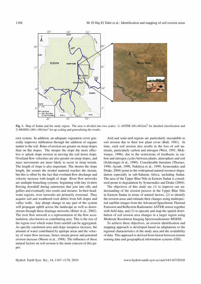
1168 M. El Haj El Tahir et al.: Identification and mapping of soil erosion areas

2

1

Fig. 1. Map of Sudan and the study region. The area is divided into two scales: 1) ASTER (60×60) km2 for detailed classification and2) MODIS (180×180) km2 for up scaling and generalizing the results.

root system. In addition, an adequate vegetation cover gen-erally improves infiltration through the addition of organicmatter to the soil. Rates of erosion are greater on steep slopesthan on flat slopes. The steeper the slope the more effec-tive is splash slope erosion in moving the soil down slope.Overland flow velocities are also greater on steep slopes, andmass movements are more likely to occur in steep terrain.The length of slope is also important. The shorter the slopelength, the sooner the eroded material reaches the stream,but this is offset by the fact that overland-flow discharge andvelocity increase with length of slope. River flow networksare multiple-branching systems, beginning with tiny rivuletsflowing downhill during rainstorms that join into rills andgullies and eventually into creeks and streams. In their head-water regions, river networks are primarily erosional. Theyacquire soil and weathered rock debris from hill slopes andvalley walls. Any abrupt change in any part of the systemwill propagate uphill across the landscape as well as down-stream through these drainage networks (Ritter et al., 2002).The river flow network is a representation of the flow accu-mulation, also known as contributing area. This is the size ofthe region over which water from rainfall can be aggregated.As specific catchment area and slope steepness increase, theamount of water contributed by upslope areas and the veloc-ity of water flow increase, hence stream power and potentialerosion increase (Moore et al., 1988). The influence of thesenatural factors on soil erosion is the main concern of this pa-per.

Arid and semi-arid regions are particularly susceptible tosoil erosion due to their low plant cover (Bull, 1981). Intime, such soil erosion also results in the loss of soil nu-trients, particularly carbon and nitrogen (West, 1991; Mok-wunye, 1996), due to the restrictions of feedbacks in car-bon and nitrogen cycles between plants, atmosphere and soil(Schlesinger et al., 1990). Considerable literature (Thornes,1990; Ayoub, 1998; Nakileza et al., 1999; Symeonakis andDrake, 2004) point to the widespread natural resource degra-dation especially in sub-Saharan Africa, including Sudan.The area of the Upper Blue Nile in Eastern Sudan is consid-ered prone to degradation by Symeonakis and Drake (2004).

The objectives of this study are (1) to improve our un-derstanding of the erosion process in the Upper Blue Nilein Eastern Sudan in terms of natural factors, (2) to identifythe erosion areas and estimate their changes using multispec-tral satellite images from the Advanced Spaceborne ThermalEmission and Reflection Radiometer ASTER sensor togetherwith field data, and (3) to upscale and map the spatial distri-bution of soil erosion area changes in a larger region usingModerate Resolution Imaging Spectroradiometer MODIS.

To achieve these objectives, an erosion identification andmapping approach is developed based on adaptations to theregional characteristics of the study area and the availabilityof data. This approach is derived from fusion between remotesensing data and geographical information systems (GIS).

Hydrol. Earth Syst. Sci., 14, 1167–1178, 2010 www.hydrol-earth-syst-sci.net/14/1167/2010/

M. El Haj El Tahir et al.: Identification and mapping of soil erosion areas 1169

2 Study area and data

2.1 Description of study area

The study area lies between latitudes 11◦ and 16◦ N and lon-gitudes 33◦ and 35◦ E (Fig. 1). It portrays different land usetypes including agriculture, forests and range areas. Agri-culture forms are small holdings, mechanized and river bankfarming. The area exhibits high land cover variability. It in-cludes for example the Ar Roseris power dam and its lake.There are a number of forests for example the Okalma forestreserve which is bound by Jabal Okalma (Jabal is the Arabicword for mountain) on the west and Jabal Zign (400 m a.s.l.)on the south east corner. Both mountains constitute a sourceof sheet floods towards the Okalma forest reserve. The forestreserve is a natural forest composed of a mixture of trees,mainly Acacia seyal and Balanites aegyptiaca plus otherspecies. There is a large variation of age groups from youngnew regeneration to large groups of forest stands. The forestis related to the surrounding societies providing diversifiedbenefits from the trees and the land. Regeneration and forestdevelopment factors are evident. Other areas are abandonedfallow land formed following abandonment of agriculturalcropping. To the south-east there is a seasonal Khor Dunya(a gully or a seasonal water course is locally known as khor),running from south west to north east until it joins the BlueNile. This khor is characterised by the presence of degradedareas, natural regeneration, human activities such as agricul-ture, pastoralism and small settlements, as well as human in-tervention to reclaim the vegetation. Gully erosion stripes offthe fertile clay soils from the degradational clay plain form-ing bad-lands known locally as “Kerib” (Mirghani, 2007).

Observed data indicate that the mean annual precipitationin 2006 was 900 mm, of which around 90% is collected dur-ing the rainy season (April–October). For erosion we are in-terested in the inter-annual and not the annual total of rainfall.The maximum two or three rainy days in 2006 are of interestbecause it is the maximum rainfall that causes erosion. Themaximum rainfall occurred on 8 and 10 May with precipita-tion levels as high as 109.2 mm and 200.6 mm, respectively.The mean annual temperature is 28.8 ◦C. The lowest dailymean temperature is 13 ◦C and is measured in December.The highest mean daily temperature is 43.8 ◦C and is mea-sured in May. The runoff coefficient is 20–30% (Ahmed etal., 2006). The year 2006 was an exceptionally wet year. Thenormal mean annual rainfall is 500 mm (Abdulkarim, 2006).

2.2 Economic impacts of gully erosion in thestudy region

Although erosion in the centre of the gully is visually ap-parent (Fig. 2), its effects are not always detectable in termsof changes in soil quality (Ward et al., 2001). This indi-cates how geomorphologically-apparent desertification (Nirand Klein, 1974; Rozin and Schick, 1996) and changes in

Fig. 2. Erosion in Khor Dunya an example of gully erosion in theBlue Nile region (Photo taken January 2007).

soil nutrient content are not necessarily congruent. Nonethe-less, a decline in soil nutrients is recorded as some of themost important soil variables, and thus is likely to signifi-cantly impact plant growth. Although the major erosion isusually in the centre of the gully in a strip that is only 5–30 m wide, most plant biomass and species diversity are aswell concentrated there (Ward and Olsvig-Whittaker, 1993).Moreover, the concentration of the water current in the cen-tral erosion gully necessarily reduces the water flow to theadjoining sides of the valley during floods. As a consequenceof this reduction in water availability, leaching of salts is re-duced (Shalhevet and Bernstein, 1968; Dan et al., 1973; Danand Yaalon, 1982; Dan and Koyumdjisky, 1987) and soilsalinity increases on the sides of the valley. Thus, even in thesoil that remains un-eroded, soil quality declines over time.

2.3 Data selection

Nowadays there is a vast reservoir of remote sensing data,some of them are freely available and easily download-able from the internet. Remote sensing data are describedin terms of spatial resolution, temporal resolution, tim-ing, section of the electromagnetic spectrum, stereo, in-terferometric or ranging capability, and usability (Kaab etal., 2005). Two types of satellite images are used in thisstudy: Advanced Spaceborne Thermal Emission and Reflec-tion Radiometer (ASTER) and Moderate Resolution ImagingSpectroradiometer (MODIS). In addition, a digital elevationmodel (DEM) provided by Shuttle Radar Topography Mis-sion (SRTM) was used. Table 1 summarises the data charac-teristics. The software used are PCI Geomatica version 10.1and ArcGIS version 9.3. In the following sections each dataset is described in detail.

www.hydrol-earth-syst-sci.net/14/1167/2010/ Hydrol. Earth Syst. Sci., 14, 1167–1178, 2010

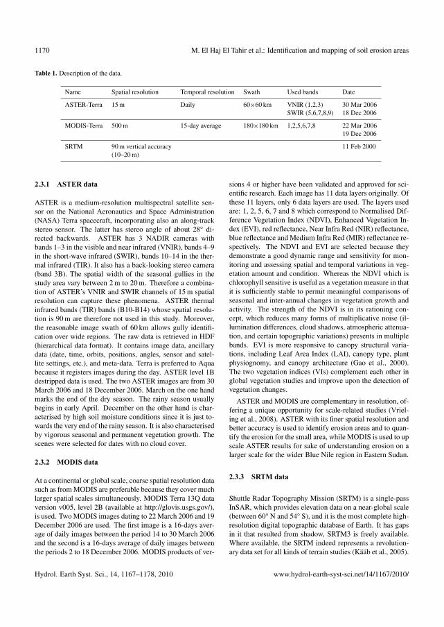
1170 M. El Haj El Tahir et al.: Identification and mapping of soil erosion areas

Table 1. Description of the data.

Name Spatial resolution Temporal resolution Swath Used bands Date

ASTER-Terra 15 m Daily 60×60 km VNIR (1,2,3) 30 Mar 2006SWIR (5,6,7,8,9) 18 Dec 2006

MODIS-Terra 500 m 15-day average 180×180 km 1,2,5,6,7,8 22 Mar 200619 Dec 2006

SRTM 90 m vertical accuracy 11 Feb 2000(10–20 m)

2.3.1 ASTER data

ASTER is a medium-resolution multispectral satellite sen-sor on the National Aeronautics and Space Administration(NASA) Terra spacecraft, incorporating also an along-trackstereo sensor. The latter has stereo angle of about 28◦ di-rected backwards. ASTER has 3 NADIR cameras withbands 1–3 in the visible and near infrared (VNIR), bands 4–9in the short-wave infrared (SWIR), bands 10–14 in the ther-mal infrared (TIR). It also has a back-looking stereo camera(band 3B). The spatial width of the seasonal gullies in thestudy area vary between 2 m to 20 m. Therefore a combina-tion of ASTER’s VNIR and SWIR channels of 15 m spatialresolution can capture these phenomena. ASTER thermalinfrared bands (TIR) bands (B10-B14) whose spatial resolu-tion is 90 m are therefore not used in this study. Moreover,the reasonable image swath of 60 km allows gully identifi-cation over wide regions. The raw data is retrieved in HDF(hierarchical data format). It contains image data, ancillarydata (date, time, orbits, positions, angles, sensor and satel-lite settings, etc.), and meta-data. Terra is preferred to Aquabecause it registers images during the day. ASTER level 1Bdestripped data is used. The two ASTER images are from 30March 2006 and 18 December 2006. March on the one handmarks the end of the dry season. The rainy season usuallybegins in early April. December on the other hand is char-acterised by high soil moisture conditions since it is just to-wards the very end of the rainy season. It is also characterisedby vigorous seasonal and permanent vegetation growth. Thescenes were selected for dates with no cloud cover.

2.3.2 MODIS data

At a continental or global scale, coarse spatial resolution datasuch as from MODIS are preferable because they cover muchlarger spatial scales simultaneously. MODIS Terra 13Q dataversion v005, level 2B (available at http://glovis.usgs.gov/),is used. Two MODIS images dating to 22 March 2006 and 19December 2006 are used. The first image is a 16-days aver-age of daily images between the period 14 to 30 March 2006and the second is a 16-days average of daily images betweenthe periods 2 to 18 December 2006. MODIS products of ver-

sions 4 or higher have been validated and approved for sci-entific research. Each image has 11 data layers originally. Ofthese 11 layers, only 6 data layers are used. The layers usedare: 1, 2, 5, 6, 7 and 8 which correspond to Normalised Dif-ference Vegetation Index (NDVI), Enhanced Vegetation In-dex (EVI), red reflectance, Near Infra Red (NIR) reflectance,blue reflectance and Medium Infra Red (MIR) reflectance re-spectively. The NDVI and EVI are selected because theydemonstrate a good dynamic range and sensitivity for mon-itoring and assessing spatial and temporal variations in veg-etation amount and condition. Whereas the NDVI which ischlorophyll sensitive is useful as a vegetation measure in thatit is sufficiently stable to permit meaningful comparisons ofseasonal and inter-annual changes in vegetation growth andactivity. The strength of the NDVI is in its rationing con-cept, which reduces many forms of multiplicative noise (il-lumination differences, cloud shadows, atmospheric attenua-tion, and certain topographic variations) presents in multiplebands. EVI is more responsive to canopy structural varia-tions, including Leaf Area Index (LAI), canopy type, plantphysiognomy, and canopy architecture (Gao et al., 2000).The two vegetation indices (VIs) complement each other inglobal vegetation studies and improve upon the detection ofvegetation changes.

ASTER and MODIS are complementary in resolution, of-fering a unique opportunity for scale-related studies (Vriel-ing et al., 2008). ASTER with its finer spatial resolution andbetter accuracy is used to identify erosion areas and to quan-tify the erosion for the small area, while MODIS is used to upscale ASTER results for sake of understanding erosion on alarger scale for the wider Blue Nile region in Eastern Sudan.

2.3.3 SRTM data

Shuttle Radar Topography Mission (SRTM) is a single-passInSAR, which provides elevation data on a near-global scale(between 60◦ N and 54◦ S), and it is the most complete high-resolution digital topographic database of Earth. It has gapsin it that resulted from shadow, SRTM3 is freely available.Where available, the SRTM indeed represents a revolution-ary data set for all kinds of terrain studies (Kaab et al., 2005).

Hydrol. Earth Syst. Sci., 14, 1167–1178, 2010 www.hydrol-earth-syst-sci.net/14/1167/2010/

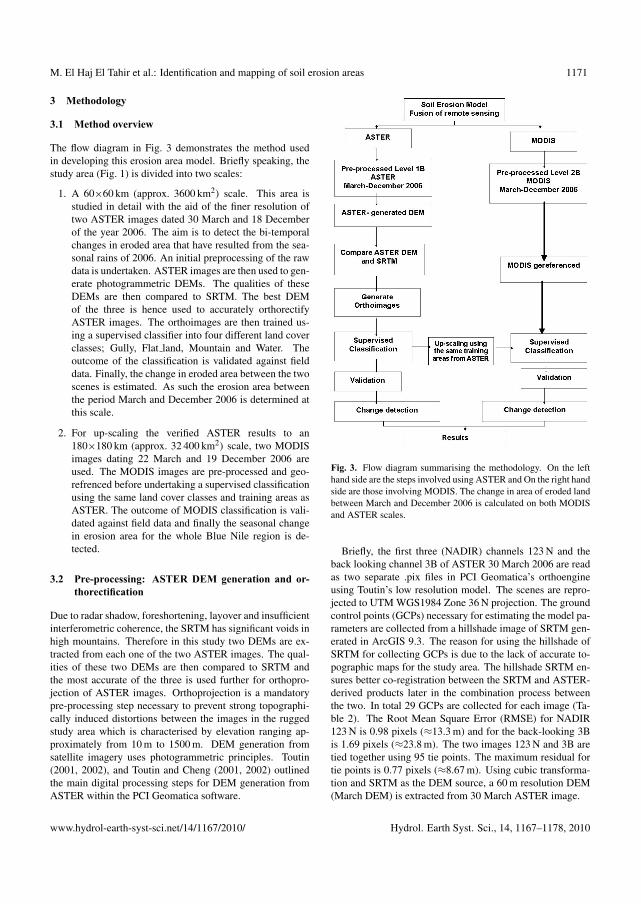
M. El Haj El Tahir et al.: Identification and mapping of soil erosion areas 1171

3 Methodology

3.1 Method overview

The flow diagram in Fig. 3 demonstrates the method usedin developing this erosion area model. Briefly speaking, thestudy area (Fig. 1) is divided into two scales:

1. A 60×60 km (approx. 3600 km2) scale. This area isstudied in detail with the aid of the finer resolution oftwo ASTER images dated 30 March and 18 Decemberof the year 2006. The aim is to detect the bi-temporalchanges in eroded area that have resulted from the sea-sonal rains of 2006. An initial preprocessing of the rawdata is undertaken. ASTER images are then used to gen-erate photogrammetric DEMs. The qualities of theseDEMs are then compared to SRTM. The best DEMof the three is hence used to accurately orthorectifyASTER images. The orthoimages are then trained us-ing a supervised classifier into four different land coverclasses; Gully, Flat land, Mountain and Water. Theoutcome of the classification is validated against fielddata. Finally, the change in eroded area between the twoscenes is estimated. As such the erosion area betweenthe period March and December 2006 is determined atthis scale.

2. For up-scaling the verified ASTER results to an180×180 km (approx. 32 400 km2) scale, two MODISimages dating 22 March and 19 December 2006 areused. The MODIS images are pre-processed and geo-refrenced before undertaking a supervised classificationusing the same land cover classes and training areas asASTER. The outcome of MODIS classification is vali-dated against field data and finally the seasonal changein erosion area for the whole Blue Nile region is de-tected.

3.2 Pre-processing: ASTER DEM generation and or-thorectification

Due to radar shadow, foreshortening, layover and insufficientinterferometric coherence, the SRTM has significant voids inhigh mountains. Therefore in this study two DEMs are ex-tracted from each one of the two ASTER images. The qual-ities of these two DEMs are then compared to SRTM andthe most accurate of the three is used further for orthopro-jection of ASTER images. Orthoprojection is a mandatorypre-processing step necessary to prevent strong topographi-cally induced distortions between the images in the ruggedstudy area which is characterised by elevation ranging ap-proximately from 10 m to 1500 m. DEM generation fromsatellite imagery uses photogrammetric principles. Toutin(2001, 2002), and Toutin and Cheng (2001, 2002) outlinedthe main digital processing steps for DEM generation fromASTER within the PCI Geomatica software.

Fig. 3. Flow diagram summarising the methodology. On the lefthand side are the steps involved using ASTER and On the right handside are those involving MODIS. The change in area of eroded landbetween March and December 2006 is calculated on both MODISand ASTER scales.

Briefly, the first three (NADIR) channels 123 N and theback looking channel 3B of ASTER 30 March 2006 are readas two separate .pix files in PCI Geomatica’s orthoengineusing Toutin’s low resolution model. The scenes are repro-jected to UTM WGS1984 Zone 36 N projection. The groundcontrol points (GCPs) necessary for estimating the model pa-rameters are collected from a hillshade image of SRTM gen-erated in ArcGIS 9.3. The reason for using the hillshade ofSRTM for collecting GCPs is due to the lack of accurate to-pographic maps for the study area. The hillshade SRTM en-sures better co-registration between the SRTM and ASTER-derived products later in the combination process betweenthe two. In total 29 GCPs are collected for each image (Ta-ble 2). The Root Mean Square Error (RMSE) for NADIR123 N is 0.98 pixels (≈13.3 m) and for the back-looking 3Bis 1.69 pixels (≈23.8 m). The two images 123 N and 3B aretied together using 95 tie points. The maximum residual fortie points is 0.77 pixels (≈8.67 m). Using cubic transforma-tion and SRTM as the DEM source, a 60 m resolution DEM(March DEM) is extracted from 30 March ASTER image.

www.hydrol-earth-syst-sci.net/14/1167/2010/ Hydrol. Earth Syst. Sci., 14, 1167–1178, 2010

1172 M. El Haj El Tahir et al.: Identification and mapping of soil erosion areas

Table 2. Generation of DEM from two ASTER images. The table summaries the root mean square error (RMSE) for the ground controlpoints (GCPs) for 123N and 3B image channel.

Image Channel GCP RMSE X RMSE Y RMSE

ASTER March Nadir 123 N 29 0.98 pixels (13.3 m) 0.81 pixel (12.00 m) 0.65 pixel (8.01 m)ASTER March Back-looking 3B 29 1.69 pixels (23.8 m) 0.87 pixel (11.90 m) 1.31 pixel (17.3 m)ASTER December Nadir 123 N 31 1.08 pixels (14.6 m) 0.84 pixel (12.06 m) 0.67 pixel (8.29 m)ASTER December Back-looking 3B 31 1.72 pixels (24.2 m) 0.91 pixel (13.0 m) 1.47 pixel (20.4 m)

The same procedure is repeated using the second ASTERimage of 18 December. The RMS is shown in Table 2. Asecond 60 m resolution DEM (December DEM) is also ex-tracted.

3.3 ASTER classification

After orthoprojecting ASTER images using SRTM, the chan-nels that best describe the process of soil erosion are selected.Considering the spatial width of gullies, ASTER’s VNIR andSWIR channels at 15 m spatial resolution have been anal-ysed. Additional layers that represent some of the mostimportant natural factors causing erosion are added. Theselayers are elevation, slope, aspect, and river flow network.Therefore the final ASTER orthoimages used for classifica-tion consisted of 13 layers stacked together. These include:VNIR channels 1, 2 and 3, SWIR channels 4, 5, 6, 7, 8 and9, SRTM, slope, aspect, and river flow network. The lastthree layers; slope, aspect and river flow network are all cal-culated from SRTM in ArcGIS 9.3. Both slope and aspectare calculated from SRTM using a finite difference methodthat uses eight neighbours in ArcGIS. The two are then re-sampled to 15 m before adding them to the layer stack. Theriver flow network was estimated using the hydrologic anal-ysis package in ArcGIS 9.3 as follows. When working withraster DEMs and computing slopes between grid cells, theratio of the vertical and horizontal resolutions determines theminimum non-zero slope that can be resolved. In this study,the vertical resolution of the DEM is 1 m and a grid sizeis 15 m. Therefore the resolvable slope of 1/15=0.07. Thisvalue means that slopes on hillsides can be computed with arelatively small error. However, slopes in channels are oftenmuch smaller than this value. As a consequence, these ar-eas will appear horizontal in the DEM. Therefore in order toavoid this problem, ArcGIS 9.3 uses an eight direction (D8)flow model. The direction of flow is determined by findingthe direction of steepest descent, or maximum drop, fromeach cell. This is calculated as

maximum drop = change in z-value/distance

The distance is calculated between cell centres. There areeight valid output directions relating to the eight adjacentcells into which flow could travel. One challenge arises if all

neighbours are higher than the processing cell. In such a casethe processing cell is called a sink and has an undefined flowdirection because any water that flows into a sink cannot flowout. To obtain an accurate representation of flow directionacross a surface, the sinks should be filled. The minimumelevation value surrounding the sink will identify the heightnecessary to fill the sink so the water can pass through thecell. A digital elevation model free of sinks is called depres-sionless DEM. Using the depressionless DEM as an inputto the flow direction process, the direction in which waterwould flow out of each cell is determined. After determin-ing the flow direction, then the flow accumulation is deter-mined. Afterwards, a stream network is created by applyinga threshold value to select cells with high accumulated flowin order delineate the stream network. More details on thetechnique of deriving flow direction from a DEM and on howto create river network in ArcGIS can be found in Jenson andDomingue (1988) and in Tang and Liu (2008), among others.

After stacking all appropriate layers, then supervised max-imum likelihood classification is performed aided by the au-thors’ knowledge of the area. The image is trained intofour land cover types: Gully, Flat land, Mountain and Wa-ter. Water bodies are clear and easy to train considering thefine ASTER resolution for both periods of the year. Moun-tains are easily classified with the aid of the DEM. However,the most challenging task is to separate between Gully andFlat land since these two classes are bound to overlap andoverlapping training area boundaries reduces the reliabilityof the training sites. To avoid this kind of overlap, the fol-lowing steps were taken

1. MODIS vegetation indices (VI) are used as auxiliarydata to discriminate between training classes; Gully andFlat land. At first MODIS NDVI and EVI signatures areused to discriminate between two classes: stable vege-tation and unstable vegetation. The unstable vegetationis seasonal vegetation that grows during the rainy sea-son; this vegetation is flushed away with erosion, indi-cating that areas where there is unstable vegetation thereis also erosion. The stable vegetation on the other handis there throughout the year hence no erosion. WhereNDVI and EVI values are low, this is an indication oflimited, unstable vegetation hence higher erosion risk.

Hydrol. Earth Syst. Sci., 14, 1167–1178, 2010 www.hydrol-earth-syst-sci.net/14/1167/2010/

M. El Haj El Tahir et al.: Identification and mapping of soil erosion areas 1173

Higher values of NDVI and EVI indicate more stablevegetation.

2. The layer of river network is superimposed on top of theimage to help guide and discriminate between Gulliesand Flat land.

3. Care is taken when selecting the different bands both fordisplay, in either greyscale or as false colour compositesFCC.

4. Between each run and the next the classes are refined byvarying the number of training areas until better accura-cies are achieved.

As many training areas as possible are trained because gen-erally speaking, the more areas identified as training sites,the higher the accuracy of the classification. Once the train-ing areas are defined, then the signature separability valuesare studied. Signature separability is the statistical differ-ence between pairs of spectral signatures. It is expressedin terms of Bhattacharrya Distance and Transformed Diver-gence. These are measures of the separability of a pair ofprobability distributions. Both Bhattacharrya Distance andTransformed Divergence are shown as real values betweenzero and two. Zero indicates complete overlap between thesignatures of two classes; two indicates a complete separa-tion between the two classes. The higher the separability (i.e.more than 1.5) value the more accurate is the classificationaccuracy. The training areas are tuned until higher signatureseparability value of 1.5 or more are achieved. After achiev-ing the best accuracies, the signature statistics report is stud-ied in order to determine which channels of the 13 stackedlayers are more significant in delineating erosion gullies.

3.4 Post classification

ASTER classification is validated via running an automaticrandom accuracy assessment. The accuracy assessment isdesigned and implemented by generating a random sampleof 300 points and comparing it to the original orthorectifiedASTER image. ASTER image is used as a reference imagedue to lack of accurate and updated maps for the study area.Each of the 300 samples is assigned to the different classes.

Once the two ASTER images are successfully classifiedand validated, they are used to study the bi-temporal change.For each image the area represented by each of the fourclasses is calculated using the function Generate Area Re-port in PCI Geomatica. The areas in December image aresubsequently subtracted from their correspondent in Marchimage in order to calculate the changed area per class.

3.5 Upscaling using MODIS

Once ASTER classification results are accepted, the resultsare then up-scaled using MODIS. Upscaling allows general-isation of the results of ASTER classification to larger area

covering the whole of the Blue Nile region. MODIS is firstre-projected to UTM WGS1984 Zone 36 N. Thereafter, it istrained into four classes; Gully, Flat land, Mountain and Wa-ter. MODIS is trained using:

1. MODIS NDVI and EVI are used as auxiliary data to dis-criminate between training classes; Gully and Flat landdiscriminating first between high values i.e. stable veg-etation i.e. no erosion and low values i.e. unstable veg-etation i.e. erosion areas.

2. The same training areas from ASTER which are con-verted into shape file and laid over the MODIS image toguide the training.

3. River flow network layer overlaid over the images toguide the training of gullies

MODIS classification is validated against field data in termsof registered digital photos with co-ordinates and time takenin January 2007 from different locations.

4 Results and discussion

4.1 Comparison of the three DEMs

Because the two generated ASTER DEMs cannot be testedagainst an existing reference DEM, they are tested throughthe overlay of different orthoimages taken from different sen-sor positions (also know as multi-incidence angle image).For 30 March ASTER, two orthoimages are produced onefor 123 N and another for 3B using March DEM. The twoorthoimages are then overlaid to test if they overlap per-fectly well pixel-by-pixel using animation flickering tech-niques. The results showed that the two did not overlap per-fectly. The explanation for this is that the used March DEMhas vertical errors which translated into horizontal shifts be-tween the orthoprojected pixels. These shifts cause the twomulti-incidence images not to overlap perfectly. Next De-cember DEM is tested in a similar manner. The results of theflickering technique showed some vertical errors. It is thenconcluded that the two ASTER DEMs both suffer verticalerrors. Accordingly SRTM is selected as “reference DEM”for all further steps. In order to quantify the error of ASTERMarch and December DEMs, their contour lines are com-pared to those of SRTM (Fig. 4a and b, respectively). The de-picted test area in the figure represents rugged high-mountainconditions with elevations of up to 1500 m a.s.l., steep rockwalls, deep shadows that are without contrast. Therefore, thetest area is considered to represent a worst case for DEMgeneration from ASTER data.

Figure 4a and b shows that the contour lines of twoASTER DEMs (dotted lines) are different to those of theSRTM (solid lines) and that this difference increases withelevation. Figure 4b shows that December DEM has more

www.hydrol-earth-syst-sci.net/14/1167/2010/ Hydrol. Earth Syst. Sci., 14, 1167–1178, 2010

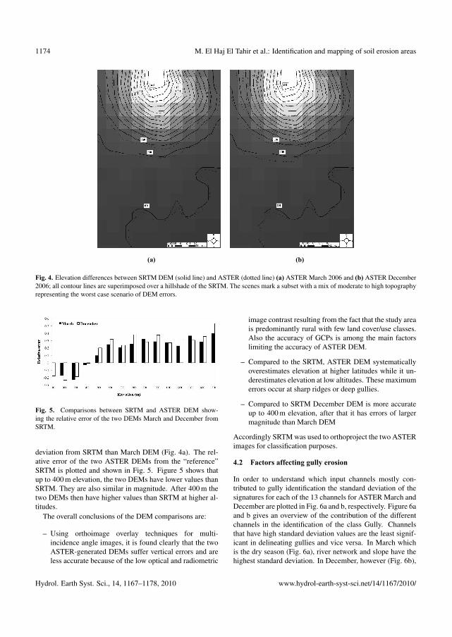
1174 M. El Haj El Tahir et al.: Identification and mapping of soil erosion areas

(a) (b)

Fig. 4. Elevation differences between SRTM DEM (solid line) and ASTER (dotted line) (a) ASTER March 2006 and (b) ASTER December2006; all contour lines are superimposed over a hillshade of the SRTM. The scenes mark a subset with a mix of moderate to high topographyrepresenting the worst case scenario of DEM errors.

Fig. 5. Comparisons between SRTM and ASTER DEM show-ing the relative error of the two DEMs March and December fromSRTM.

deviation from SRTM than March DEM (Fig. 4a). The rel-ative error of the two ASTER DEMs from the “reference”SRTM is plotted and shown in Fig. 5. Figure 5 shows thatup to 400 m elevation, the two DEMs have lower values thanSRTM. They are also similar in magnitude. After 400 m thetwo DEMs then have higher values than SRTM at higher al-titudes.

The overall conclusions of the DEM comparisons are:

– Using orthoimage overlay techniques for multi-incidence angle images, it is found clearly that the twoASTER-generated DEMs suffer vertical errors and areless accurate because of the low optical and radiometric

image contrast resulting from the fact that the study areais predominantly rural with few land cover/use classes.Also the accuracy of GCPs is among the main factorslimiting the accuracy of ASTER DEM.

– Compared to the SRTM, ASTER DEM systematicallyoverestimates elevation at higher latitudes while it un-derestimates elevation at low altitudes. These maximumerrors occur at sharp ridges or deep gullies.

– Compared to SRTM December DEM is more accurateup to 400 m elevation, after that it has errors of largermagnitude than March DEM

Accordingly SRTM was used to orthoproject the two ASTERimages for classification purposes.

4.2 Factors affecting gully erosion

In order to understand which input channels mostly con-tributed to gully identification the standard deviation of thesignatures for each of the 13 channels for ASTER March andDecember are plotted in Fig. 6a and b, respectively. Figure 6aand b gives an overview of the contribution of the differentchannels in the identification of the class Gully. Channelsthat have high standard deviation values are the least signif-icant in delineating gullies and vice versa. In March whichis the dry season (Fig. 6a), river network and slope have thehighest standard deviation. In December, however (Fig. 6b),

Hydrol. Earth Syst. Sci., 14, 1167–1178, 2010 www.hydrol-earth-syst-sci.net/14/1167/2010/

M. El Haj El Tahir et al.: Identification and mapping of soil erosion areas 1175

Fig. 6. The contribution of the different input channels in delineat-ing gullies in ASTER images (a) March, (b) December.

Table 3. Classification report of ASTER images.

Image Average Overall Kappaaccuracy accuracy coefficient

ASTER March 93.4% 82.2% 0.82ASTER December 87% 75.2% 0.75

they have the lowest standard deviation values and hence theyare the most important in Gully classification. During andafter the rainy season, river network and slope are the mostimportant factors in the erosion process. In December rivernetworks continue to flow even when the rain has stoppedcarrying with the flow soil and weathered rock debris fromhill slopes and valley walls and as slope steepness increase,the amount of water contributed by upslope areas and the ve-locity of water flow increase, hence stream power and poten-tial erosion increase. As natural factors, river flow networkand slope are more important in causing erosion in the BlueNile region than aspect and elevation.

4.3 Validation of the classification outcome

ASTER classification reports (Table 3) shows an overall ac-curacy of 82.2% and 75.2% for March and December im-ages, respectively. And similarly for ASTER validation, the

Validation points

Fig. 7. Regional spatial distribution map of seasonal gullies of theBlue Nile, Eastern Sudan.

accuracy assessment report (Table 4) shows that in March theoverall accuracy is 93% and in December is 89%. The clas-sification of March image is better than December becauseVNIR and SWIR channels are more capable of discriminat-ing erosion gullies in the dry season due to higher spectralreflectance.

MODIS classification accuracies for March and Decem-ber are 77.2% and 81.0% respectively (Table 5). Automaticaccuracy assessment (Table 6) shows overall accuracies of89% and 88.7% for March and December, respectively. Ad-ditionally, the classified MODIS image is validated againsta set of thirteen digital photos taken in the field. Nine val-idation points showed gullies coinciding with the results ofthe classification (Fig. 7). In March classification is betterthan that of December because in the dry season there is lesssoil moisture therefore higher surface reflectance. The over-all accuracy of MODIS is less than that of ASTER. The rea-sons are that there is insufficient spectral distinctiveness dueto the low spectral and spatial resolution of the MODIS data;MODIS products consisted of averaged products rather thanthe actual spectral bands; some artefacts interfered with thecalculation of eroded areas.

4.4 Estimation of soil erosion on ASTER scale

The results of the bi-temporal change of gully erosion inASTER scale are shown in Table 7. Table 7 shows an in-crease by approximately 112 km2 in the area of gullies. Thisis because after the rainy season, both rain and flood water

www.hydrol-earth-syst-sci.net/14/1167/2010/ Hydrol. Earth Syst. Sci., 14, 1167–1178, 2010

1176 M. El Haj El Tahir et al.: Identification and mapping of soil erosion areas

Table 4. Validation of ASTER classification: accuracy statistics report indicating the outcome of the accuracy assessment of the usedsupervised maximum likelihood classifier.

ASTER March

Class name Producer’s accuracy User’s accuracy Kappa statistic

Mountain 88.2% 97.8% 0.97Gully 92.2% 92.2% 0.90Flat 96.3% 92.3% 0.83Water 70.0% 87.5% 0.87

Overall accuracy 93.0%

ASTER December

Class Name Producer’s accuracy User’s accuracy Kappa statistic

Mountain 69.2% 75.0% 0.74Gully 87.0% 85.3% 0.78Flat 95.2% 79.7% 0.75Water 91.7% 100% 1.00

Overall accuracy 89.0%

Table 5. Classification report of MODIS products.

Image Average Overall Kappaaccuracy accuracy coefficient

MODIS March 77.2% 61.9% 0.40MODIS December 81.0% 63.8% 0.20

dissects large areas creating either new gullies or increasingthe width and/or depth of existing gullies. Naturally an in-crease in dissected land reduces the extent of flat land. Thatis why there is a decrease of flat land by about 153 km2. Thearea covered with water has increased by 31.5 km2. That isdue to the fact that in December there are still large areas thatare covered with rain and flood water from the rainy seasontime which have not receded, percolated or evaporated yet.The total area classified as mountains did not change. In factthis is regarded as an indication of the success of the classi-fication because when stable features like mountains remainstable then this is regarded as an indication of good georefer-encing and subsequently good multitemporal analysis (Kaab,2005).

4.5 Estimation of erosion on a regional scale

The change in the total area of gullies is estimated by sub-tracting the area in MODIS December image from that inMODIS March (Table 8). Table 8 shows that gullies have in-creased by approximately 2071 km2, and water by 1791 km2,respectively. Flat land has decreased by 3864 km2 whilemountains remained unchanged. Hence the estimated areaalong the Blue Nile River, Eastern Sudan that was affectedby soil erosion during the 2006 rainy season was estimated to

be 2071 km2 or 6.5% of the total study area approximately.This estimation should be viewed in light of the facts that:(a) the year 2006 was exceptionally wet year compared toprevious years, (b) the Upper Blue Nile River is steeper andreceives more rain than any other river in Sudan namely, theWhite Nile, River Atbara, Sobat, etc., and (c) there has notbeen any previous studies reported in this region.

After close comparison and evaluation of the soil erosionmodel as presented above, it is used to map the spatial distri-bution of gully erosion in the Blue Nile region during 2006seasonal rains (Fig. 7). It is seen in the figure that gully ero-sion is evident in and around the Blue Nile River and its trib-utaries.

5 Summary and conclusion

Soil erosion poses a serious environmental and socio-economic threat to the environment and to mankind. Previ-ous research in sub-Sahara Africa has singled out the UpperBlue Nile as an erosion prone area that is recommended forfurther monitoring and evaluation. In this study a soil erosionarea model is suggested. The model benefits from advancesin GIS and remote sensing fusion techniques. The modelis simple, robust and straightforward. It makes use of thewell tested methods of supervised classification using maxi-mum likelihood (MLC). Generalisation of ASTER classifica-tion results using MODIS was useful for capturing a regionalimpression of the spatial distribution of erosion. Key to themodel’s success is further development of proper validationprocedures. The size of this region makes the traditionalmapping methods of aerial photography and field surveyingof limited use. Moderate resolution multispectral data allowscontinental- to global-scale mapping of the Earth’s surface

Hydrol. Earth Syst. Sci., 14, 1167–1178, 2010 www.hydrol-earth-syst-sci.net/14/1167/2010/

M. El Haj El Tahir et al.: Identification and mapping of soil erosion areas 1177

Table 6. Validation of MODIS classification: accuracy statistics report indicating the outcome of the accuracy assessment of the usedsupervised classifier.

MODIS March

Class name Producer’s accuracy User’s accuracy Kappa statistic

Mountain 94.1% 80.0% 0.76Gully 90.6% 93.6% 0.91Flat 89.7% 89.7% 0.83Water 75.0% 90.0% 0.89

Overall accuracy 89.0%

MODIS December

Class name Producer’s accuracy User’s accuracy Kappa statistic

Mountain 91.2% 80.0% 0.74Gully 87.6% 92.5% 0.88Flat 85.7% 89.9% 0.70Water 72.6% 91.4% 0.89

Overall accuracy 88.7%

Table 7. Local change of erosion area as indicated by the differ-ence (diff) in area percentage (%) or in km2 between March andDecember 2006 for the four land cover classes.

ClassArea (%) Area (km2)

Mar Dec Diff Mar Dec Diff

Gully 42.1 50.9 8.77 538.5 650.7 112.2Flat land 46.6 34.63 −12 596 442.9 −153.1Mountain 4.43 4.43 0.00 56.7 56.701 0.05Water 6.87 10.07 3.20 67.9 99.49 31.59

Table 8. Regional change of erosion area as indicated the differ-ence (diff) in area percentage (%) or in km2 between March andDecember 2006 for the four land cover classes.

ClassArea (%) Area (km2)

Mar Dec Diff Mar Dec Diff

Gully 33.1 39.7 6.55 10 467 12 538 2071Flat land 39.8 27.6 −12.2 12 572 8708 −3864Mountain 21.3 21.3 0 6737 6737 0Water 5.84 11.5 5.67 1845 3636 1791

while retaining sufficient resolution for geomorphic and eco-logical studies.

The following conclusions are drawn from the study:

1. ASTER-derived DEMs are less accurate than SRTM be-cause of the low optical contrast of the study area whichis predominantly rural with few land cover/use classeslow.

2. The incision of gullies found in this area is stronglyassociated with topography, especially river flow net-works and slope.

3. Moreover, on-going climate change can initiate newprocesses via increased rainfalls, or weaken land cover.

The model can be used to study longer-term changes in ero-sion by using time series of images from different years. Themethodology presented here is also transportable to otherarid and semi-arid parts of Sudan where an understandingof soil erosion is desirable.

Acknowledgements. Our appreciation extends to the NorwegianResearch Council (NFR) for sponsoring the project number 171783(FRIMUF), Department of Geosciences, University of Oslo,Faculty of Engineering, University of Khartoum, The Forestry,Irrigation and Environment National Corporations of Sudan.

Edited by: N. Romano

References

Abdulkarim, A.: Rainfall variability in the Blue Nile state, in: Re-ports of the National Meteorological Office, Khartoum, Sudan,2006.

Ahmed, A., Osman, I., and Babiker, A.: Sediment and AquaticWeeds Management Challenges in Gezira Irrigated Scheme in:Proceedings, UNESCO’s International Sediment Initiative Con-ference (ISIC), Khartoum, Sudan, 12–15 November 2006.

Ayoub, A. T.: Extent, Severity and Causative Factors of LandDegradation in Sudan, J. Arid Environ., 38, 397–409, 1998.

Bull, W. B.: Soils, geology, and hydrology of deserts, in: Water indesert ecosystems, edited by: Evans, D. D. and Thames, J. L.,Stroudsberg, Pa, Dowden, Hutchinson and Ross, USA, 42–58,1981.

Dan, J. and Koyumdjisky, H.: Distribution of salinity in the soils ofIsrael, Israel J. Earth Sci., 36, 213–223, 1987.

www.hydrol-earth-syst-sci.net/14/1167/2010/ Hydrol. Earth Syst. Sci., 14, 1167–1178, 2010

1178 M. El Haj El Tahir et al.: Identification and mapping of soil erosion areas

Dan, J. and Yaalon, D. H.: Automorphic saline soils in Israel, in:Aridic soils and geomorphic processes, edited by: Yaalon, D. H.,Cathena Verlag, 1, Braunschweig, Germany, 103–115, 1982.

Dan, J., Moshe, R., and Alperovitch, N.: The soils of Sede Zin,Israel J. Earth Sci., 22, 211–227, 1973.

Gao, X., Huete, A., Ni, W., and Miura, T.: Optical –biophysicalrelationships of vegetation spectra without background contami-nation, Remote Sens. Environ., 74, 609–620, 2000.

Gomer, D. and Vogt, T.: Physically based modelling of surfacerunoff and soil erosion under semi-arid Mediterranean condi-tions, the example of Oued Mina, Algeria, in: Soil Erosion:Application of Physically based models, edited by: Schmidt, J.,Springer Verlag, Berlin, Heidelberg, New York, 58–78, 2000.

Jenson, S. K. and Domingue, J. O.: Extracting Topographic Struc-ture from Digital Elevation Data for Geographic InformationSystem Analysis, Photogrammetric Engineering and RemoteSensing, 54(11), 1593–1600, 1988.

Kaab, A., Huggel, C., Fischer, L., Guex, S., Paul, F., Roer, I., Salz-mann, N., Schlaefli, S., Schmutz, K., Schneider, D., Strozzi, T.,and Weidmann, Y.: Remote sensing of glacier- and permafrost-related hazards in high mountains: an overview, Nat. HazardsEarth Syst. Sci., 5, 527–554, doi:10.5194/nhess-5-527-2005,2005.

Kaab, A.: Combination of SRTM3 and repeat ASTER data forderiving alpine glacier flow velocities in the Bhutan Himalaya,Rem. Sens. Environ., 94(4), 463–474, 2005.

Linsely, R. K., Kohler, M. A., and Paulhus, J. L. H.: Hydrol-ogy for Engineers, Third Edition, International Student Edition,McGraw-Hill Kogakusha, Ltd, New Delhi, India, 1982.

Mirghani, O.: Report on the Field Visit to Sennar and Blue NileStates, in: Field work report, 2007.

Mokwunye, U.: Nutrient depletion: sub-Saharan Africa’s greatestthreat to economic development, S.T.A.P. expert workshop onLand Degradation Dakar, Senegal, 1996.Moore, I. D., O’Loughlin, E. M., and Burch, G. J.: A contour-based topographic model for hydrological and ecological appli-cations, Earth Surf. Processes Landforms, 3(4), 305–320, 1988.

Nakileza, B., Nsubuga, E., Tenywa, M., and Lwakuba, A.: Rethink-ing Natural Resource Degradation in Semi-Arid Sub-SaharanAfrica: A review of soil and water conservation research andpractice in Uganda, with particular emphasis on the semi- aridareas, Overseas Development Institute (ODI) Report, 1999.

Nearing, M. A., Pruski, F. F., and O’Neal, M. R.: Expected cli-mate change impacts on soil erosion rates, a review, J. Soil WaterConservation, 59(1), 43–50, 2004.

Nir, D. and Klein, M.: Gully erosion induced in land size in a semi-arid terrain (Nahal Shiqma, Israel), Zeitschrift fur Geomorpholo-gie, 21, 191–201, 1974.

Ritter, F., Kochel, R., and Miller, J.: Process Geomorphology, 4thEd., McGraw-Hill, New York, 2002.

Rozin, U. and Schick, A.: Land use change, conservation measuresand stream channel response in the Mediterranean/semiarid tran-sition zone: Nahal Hoga, southern coastal plain, Israel, in: Ero-sion and sediment yield global and regional perspectives, IAHSpubl., 236, 427–443, 1996.

Schlesinger, W., Reynolds, J. F., Cunningham, G. L., Huenneke, L.F., Jarrell, W. M., Virginia, R. A., and Whitford, W. G.: Biologi-cal feedbacks in global desertification, Science, 247, 1043–1048,1990.

Shalhevet, J. and Bernstein, L.: Effects of vertically heterogeneoussoil salinity on plant growth and water uptake, Soil Science, 106,85-93, 1968.

Symeonakis, E. and Drake, N.: Monitoring Desertification andLand Degradation over Sub- Saharan Africa, Int. J. Rem. Sens.,25(3), 573–592, 2004.

Tang, C. and Liu, C.: Surface water hydrologic simulationof Qingshuijiang Watershed based on SRTM DEM, Proc.The International Society for Optical Engineering SPIE, 7143,doi:10.1117/12.812556, 2008.

Thornes, J. B.: The interaction of erosional and vegetation dynam-ics in land degradation: spatial outcomes, in: Vegetation and Ero-sion, edited by: Thornes, J. B., Chichester, John Wiley, 41–53,1990.

Toutin, T. and Cheng, P.: Comparison of automated digital elevationmodel extraction results using along-track ASTER and across-track SPOT stereo images, Optical Engineering, 41(9), 2102–2106, 2002.

Toutin, T. and Cheng, P.: DEM generation with ASTER stereo data,Earth Observation Magazine, 10(6), 10–13, 2001.

Toutin, T.: DEM generation from new VIR Sensors, IKONOS,ASTER and Landsat 7 Proceedings, IGARSS 01, Sydney, Aus-tralia 2001.

Toutin, T.: Three-dimensional topographic mapping with ASTERstereo data in rugged topography, IEEE Trans. Geosci. Rem.Sens., 40, 10, 2241–2247, 2002.

Vrieling, A., Jong, S., Sterk, G., and Rodrigues, S.: Timing of ero-sion and satellite data: A multi-resolution approach to soil ero-sion risk mapping, Int. J. Appl. Earth Obs., 10, 267–281, 2008.

Ward, D. and Olsvig-Whittaker, L.: Plant species diversity at thejunction of two desert biogeographic zones, Biodiversity Lett.,1, 172–185, 1993.

Ward, D., Feldman, K., and Avni, Y.: The effects of erosion loesson soil nutrients, plant diversity and plant quality in Negev desertwadis, J. Arid Environ., 48, 461–473, 2001.

West, N. E.: Nutrient cycling in soils of semiarid and arid regions,in: Semiarid Lands and Deserts: Soil Resource and Rehabili-tation, edited by: Skujins, J., Marcel Dekker, Inc., New York,295–332, 1991.

Xu, C-Y., Zhang, Q., El Hag El Tahir, M., and Zhang, Z.: Statisticalproperties of the temperature, relative humidity, and solar radi-ation in the Blue Nile- Eastern Sudan region, J. Theoret. Appl.Climatol., doi:10.1007/00704009-0225-7, 2009.

Hydrol. Earth Syst. Sci., 14, 1167–1178, 2010 www.hydrol-earth-syst-sci.net/14/1167/2010/

II

III

IV

V

ORIGINAL PAPER

Spatial and temporal variation of precipitation in Sudan and theirpossible causes during 1948–2005

Zengxin Zhang • Chong-Yu Xu •

Majduline El-Haj El-Tahir • Jianrong Cao •

V. P. Singh

Published online: 3 July 2011

� The Author(s) 2011. This article is published with open access at Springerlink.com

Abstract Temporal and spatial patterns of precipitation

are essential to the understanding of soil moisture status

which is vital for vegetation regeneration in the arid eco-

systems. The purposes of this study are (1) to understand

the temporal and spatial variations of precipitation in

Sudan during 1948–2005 by using high quality global

precipitation data known as Precipitation REConstruction

(PREC), which has been constructed at the National Oce-

anic and Atmospheric Administration (NOAA) Climate

Prediction Center, and (2) to discuss the relationship

between precipitation variability and moisture flux based

on the NCEP/NCAR reanalysis data in order to ascertain

the potential causes of the spatial and temporal variations

of precipitation in the region. Results showed that (1)

annual and monthly precipitation in Sudan had great spatial

variability, and mean annual precipitation varied from

almost nil in the North to about 1500 mm in the extreme

Southwest; (2) precipitation of the main rain season, i.e.,

July, August and September, and annual total precipitation

in the central part of Sudan decreased significantly during

1948–2005; (3) abrupt change points were found in the

annual, July, August and September in the late 1960s, when

precipitation decreased more rapidly than in other periods;

and (4) the decreasing precipitation was associated with the

weakening African summer monsoon. The summer mois-

ture flux over Sudan tended to be decreasing after the late

1960s which decreased the northward propagation of

moisture flux in North Africa. This study provides a

complementary view to the previous studies that attempted

to explain the Sahel persistent drought and possible causes.

Keywords Precipitation � Large scale � Abrupt �Moisture flux � Sudan � African monsoon

1 Introduction

In recent years, droughts and subsequent famine and dis-

ease have devastated Africa and affected millions of peo-

ple. With much of rural Africa already struggling to obtain

adequate fresh water supplies, the drier conditions and

altered precipitation patterns will make meeting the water

needs of some of the poorest Africans much harder.

Rainfall is the most important water resource in Sudan.

However, low levels of rainfall have affected Sudan and

resulted in severe droughts in recent years. The years 1983

and 1984 were the most difficult years for the region in

recent history (Eltahir 1992). In 1984, crop failure and the

spread of water-borne diseases caused by the drought took

the lives of 55,000 people which weakened the socioeco-

nomic capabilities of the nomadic tribes in Sudan (Osman

and Shamseldin 2002).

Z. Zhang

Jiangsu Key Laboratory of Forestry Ecological Engineering,

Nanjing Forestry University, Nanjing 210037, China

C.-Y. Xu (&) � M. E.-H. El-Tahir

Department of Geosciences, University of Oslo, P.O. Box 1047

Blindern, 0316 Oslo, Norway

e-mail: chongyu.xu@geo.uio.no

C.-Y. Xu

Department of Earth Sciences, Uppsala University,

Uppsala, Sweden

J. Cao

College of Environment and Planning, Liaocheng University,

Liaocheng 251059, China

V. P. Singh

Department of Civil and Environmental Engineering, Texas

A&M University, College Station, TX 77843-2117, USA

123

Stoch Environ Res Risk Assess (2012) 26:429–441

DOI 10.1007/s00477-011-0512-6

In Sudan, the rain-fed agriculture produces food for 90%

of the population. Rainfall is caused by the southwesterly

monsoon winds flowing from the Atlantic Ocean and the

southeasterly monsoon winds flowing from the Indian

Ocean (Osman and Shamseldin 2002). To ascertain the

precipitation change and its possible cause in Sudan during

the past decades, several observational studies, using

meteorological data, point to the climate change in Sudan

and these studies confirm that the temperature is rising and

rainfall is declining for the past several decades which

might accelerate environmental degradation and desertifi-

cation in Sudan (e.g., Alvi 1994; Janowiak 1988; Nichol-

son et al. 2000). The precipitation anomaly of Sudan has

been related to Sea Surface Temperature Anomalies

(SSTAs) in the Gulf of Guinea (Lamb 1978a, b). Palmer

(1986) has pointed out that the tropical Indian Ocean SST

has a strong influence on the Sahel rainfall. Camberlin

(1995) found that the dry and wet conditions over the Sahel

were usually associated with warm conditions in the trop-

ical Indian Ocean. Osman and Shamseldin (2002) also

investigated the influence of El Nino-southern oscillation

(ENSO) and the Indian Ocean Sea surface temperature

(SST) on the rainfall variability in the central and southern

regions of Sudan and found that the driest years were

associated with warm ENSO and Indian Ocean SST con-

ditions. Comprehensive analysis and reviews of rainfall

trends and variability in Africa, including the Sahel region

and Sudan had been carried out by Hulme and his co-

authors (e.g., Trilsbach and Hulme 1984; Hulme 1987,

1990; Hulme and Tosdevin 1989; Walsh et al. 1988).

Trilsbach and Hulme (1984) examined rainfall changes and

their physical and human implications in the critical

desertification zone between latitudes 128N and 168N of

the Democratic Republic of Sudan and concluded, among

others, that heavy falls of rain ([40 mm) are more likely to

decline than medium ([10 mm) and light (\10 mm) falls.

Walsh et al. (1988) reported that ‘‘rainfall decline in semi-

arid Sudan since 1965 has continued and intensified in the

1980 s, with 1984 the driest year on record and all annual

rainfalls from 1980 to 1987 well below the long-term

mean’’. Hulme (1990) reported that rainfall depletion has

been most severe in semi-arid central Sudan between

1921–1950 and 1956–1985. The length of the wet season

has contracted, and rainfall zones have migrated south-

wards. A reduction in the frequency of rain events rather

than a reduced rainfall yield per rain event was found to be

the main reason for this depletion.

Increasingly the tendency has been for studies examin-

ing the causes of droughts, to look at global scales through

the notion of teleconnections. It would seem reasonable

that the current drought is a manifestation of an interaction

of two or more mechanisms (Cook and Vizy 2006).

Nicholson (1986) pointed out that the variations in the

Sahel rainfall are generally related to the changes in the

intensity of the rainy season rather than to its onset or

length as the ITCZ hypothesis would require.

Drought implies some form of moisture deficit and

moisture plays an important role in understanding climate

change (Prueger et al. 2004). Vertically integrated moisture

flux and its convergence/divergence are closely related to

precipitation. Much research work has been performed

regarding the moisture flux over Africa (e.g., Cadet and

Nnoli 1987; Fontaine et al. 2003; Osman and Hastenrath

1969). Cadet and Nnoli (1987) pointed out that the pro-

gressive penetration of moisture over West Africa during

summer at 850 hPa and the southerly flow penetrates up to

20�N during the maximum activity of the African monsoon.

Hulme and Tosdevin (1989) assessed the relationship

between tropical easterly jet (TEJ) and Sudan rainfall and

found changes in the dynamics and flow of the TEJ exert

some control over the Sahelian rainfall. Fontaine et al.

(2003) analyzed the atmospheric water and moisture fluxes

in West African Monsoon based on NCEP/NCAR and

observed rainfall data and found that at more local scales

moisture advections and convergences are also significantly

associated with the observed Sudan-Sahel rainfall and in

wet (dry) situations, with a clear dominance of westerly

(easterly) anomalies in the moisture flux south of 15�N.Although many studies have attempted to explain the

Sahel persistent drought in terms of general circulation

features, sea surface temperatures, land surface feedback

mechanisms, and teleconnected, spatiotemporal rainfall

patterns. However, the cause of the Sahel drought remains

elusive (Nicholson 1989; Rowell et al. 1995; Long et al.

2000; Trilsbach and Hulme 1984). Long et al. (2000) aimed

to advance the understanding of these causes by examining

rainfall, horizontal moisture transport, and vertical motion

and how they differ regionally and seasonally. There are a

few previous studies that have looked at how the precipi-

tation variability is related to the moisture flux in Sudan.

The main aim of this study is to provide a complementary

view to the previous studies by examing the relationship of

moisture flux and precipitation trend in the region. The

specific objectives of the study are: (1) to understand the

spatial and temporal variability of precipitation from Pre-

cipitation REConstructed (PREC) data in Sudan during

1948–2005; and (2) to investigate the relationship between

precipitation and moisture flux in the region.

2 Study area and data

Sudan is a vast country with an area of about 2.5 mil-

lion km2 and has an estimated population of about 41.1

million people. The climate ranges from arid in the north to

tropical wet-and-dry in the far southwest. About two-thirds

430 Stoch Environ Res Risk Assess (2012) 26:429–441

123

of Sudan lies in the dry and semi-dry region. Temperatures

do not vary greatly with the season at any location; the

most significant climatic variables are rainfall and the

length of the rainy season. Except in the northeast region,

from January to March, the country is under the influence

of dry northeasterly winds, and during this period there is

almost no rainfall countrywide except for a small area in

north eastern Sudan where the winds pass over the Medi-

terranean bringing occasional light rains. By early April,

rainy season starts from southern Sudan as the moist south

westerlies reach the region, and by August the southwest-

erly flows extend to the northern limits. The dry north-

easterlies begin to strengthen in September and to push

south and cover the entire country by the end of December.

In this paper, we use the global monthly precipitation

data (PREC) created by Chen et al. (2002) instead of

NCEP/NCAR precipitation data, because previous studies

have shown that the NCEP/NCAR reanalysis precipitation

exhibits some deficiencies and that this field does not

compare as well with observations as other reanalysis

fields, such as heights, winds, and temperatures that are

assimilated directly into the model (Poccard et al. 2000;

Janowiak et al. 1998). Monthly precipitation data have

been selected from the global precipitation reconstruction

data (PREC) estimates on a 0.5 9 0.5� latitude/longitude

grid over the period 1948–2005 in Sudan, which has in

total 890 grids. The PREC analyses are derived from gauge

observations from over 17,000 stations collected in the

Global Historical Climatology Network (GHCN), version

2, and the Climate Anomaly Monitoring System (CAMS)

datasets. The global analyses are defined by interpolation

of gauge observations over land (PREC/L) and by using

empirical orthogonal functions (EOF) for interpolation and

subsequent reconstruction of historical observations over

ocean (PREC/O) (Chen et al. 2002). Shi et al. (2002a, b,

2004) analyzed the global land precipitation dataset

(PREC/L) and found that this dataset was accurate enough

for describing the change of large scale precipitation, and

there was a good relationship between the global precipi-

tation database (PREC) and observed Western Africa

monsoon precipitation during 1948–2001. In the Northern

Hemisphere, the tropical area to the south of 25�N, pre-cipitation showed a negative trend in all seasons. For

comparison, long-term mean monthly precipitation dataset

from 39 observed rain gauge stations from GHCH Ver-

sion 2 were also used in this study. The location of Sudan

and observed and reconstructed grid points can be refer-

red to Fig. 1 and Table 1. Figure 1 shows that the PREC

data has, in general, a good agreement with observed

data. In the rest of the paper detailed analysis is only done

for the PREC data, because the observed data has too few

stations and only 12 long-term mean monthly values are

available.

Atmospheric data from NCEP/NCAR-I reanalysis (R-1)

over the period 1948–2005 are available on a 2.5 9 2.5�latitude/longitude grid. The water vapor flux of the whole Ps

layer (surface pressure) -300 hPa was analyzed in this

study. In the actual atmosphere, themoisture is very low over

300 hPa, so p = 300 hPa will be used in the calculation.

3 Methods

The Mann–Kendall trend test (MK; Mann 1945; WMO

1966; Kendall 1975; Sneyers 1990) is widely used in the

literature to analyze trends in the climate data. The MK test

has different variants. In this study two different versions

are used for two different purposes. The procedure of the

first version as demonstrated by Zhang et al. (2010a) starts

by simply comparing the most recent data with earlier

values. A score of ?1 is awarded if the most recent value is

larger, or a score of -1 is awarded if it is smaller. The total

score for the time-series data is the Mann–Kendall statistic,

Z, which is then compared to a critical value, Z1-a/2 (where

a is significance level, and Z1-a/2 is the Z value found in the

standard normal distribution table), to test whether the

trend in the data is significantly increasing (Z[ Z1-a/2),

significantly decreasing (Z\-Z1-a/2) or if no trend

(-Z1-a/2\ Z\Z1-a/2). This procedure is used to produce

results as showed in Figs. 4 and 7, and in Table 2.

In contrast to the traditional MK test which calculates

above statistic variables only once for the whole sample,

MK method can also be used to test an assumption

regarding the beginning of the development of a trend

within a sample, i.e., a changing point in the time series

(Zhang et al. 2009). Following the procedure as shown by

Gerstengarbe and Werner (1999) who used the method to

test an assumption about the beginning of the development

of trend within a sample (x1, x2,…, xn) of the random

variable X, the corresponding rank series for the so-called

retrograde rows are similarly obtained for the retrograde

sample (xn, xn-1,…, x1). Based on the rank series r of the

progressive and retrograde rows of this sample, the statistic

variables, Z1 and Z2 will be calculated for the progressive

and retrograde samples, respectively. The Z1 and Z2 values

calculated with progressive and retrograde series are named

UF and UB, respectively, in this paper. The intersection

point of the two lines, UF and UB gives the point in time of

the beginning of a developing trend within the time series.

This method is used to produce results as showed in Fig. 5b.

As a complementary method of trend analysis, simple

linear regression was also used in this paper for long-term

linear trend test. The simple linear regression method is a

parametric T-test method, which consists of two steps,

fitting a linear simple regression equation with the time t as

independent variable and the hydrological variable (i.e.

Stoch Environ Res Risk Assess (2012) 26:429–441 431

123

precipitation and moisture flux in this study) Y as depen-

dent variable; testing the statistical significance of the slope

of the regression equation by the t-test (Xu 2001; Zhang

et al. 2010a). The parametric T-test requires the data to be

tested is normally distributed. The normality of the data

series is first tested in the study by applying the Kol-

mogorov–Smirnov test. The T-test method is used to pro-

duce the results as showed in Figs. 5a and 9.

It is evident that the power of the test to detect the

existing trend is significantly influenced by, among others,

serial correlation in the time series and sample size or

record length. The larger the sample size, the more pow-

erful the test. Therefore, the assessment results of time

series with different record length should not be put toge-

ther to infer a general trend tendency (Yue and Wang

2002a, b). In this study, the data length of rainfall for all the

grid points is 58 years (1948–2005). In this study, the

influence of serial correlation in the time series on the

results of MK test was eliminated by prewhitening

(e.g., Yue et al. 2002; Yue and Wang 2002a, b). ‘‘Pre-

whitening’’ is one of the methods used to prevent false

indication of trend, where autocorrelation is removed from

the data by assuming a certain correlation model, usually a

Markovian one (e.g., Von Storch 1995).

The zonal moisture transport flux (QU) and meridional

moisture transport flux (QV) were calculated based on the

following equations (Cadet and Nnoli 1987; Zhou et al.

1998):

Quðx; y; tÞ ¼ 1

g

Zpps

qðx; y; p; tÞuðx; y; p; tÞdp ð1Þ

Qvðx; y; tÞ ¼ 1

g

Zpps

qðx; y; p; tÞvðx; y; p; tÞdp ð2Þ

36°E

36°E

32°E

32°E

28°E

28°E

24°E

24°E

22°N

22°N

18°N

18°N

14°N

14°N

10°N

10°N

6°N

6°N

2°N

2°N000,10 500

Km

1 2 3 4 5 6 7 8 9 10 11 120

30

60

90

120

150

180

210

240

prec

ipita

tion

(mm

)

Prec Obs

Geneina station

1 2 3 4 5 6 7 8 9 10 11 120

306090

120150180210240270

prec

ipita

tion

(mm

)

Prec Obs

Raga station

1 2 3 4 5 6 7 8 9 10 11 1205

101520253035404550

prec

ipita

tion

(mm

)

h

Prec Obs

Aqiq station

1 2 3 4 5 6 7 8 9 10 11 120

102030405060708090

prec

ipita

tion

(mm

) Prec Obs

Khartoum station

1 2 3 4 5 6 7 8 9 10 11 120

20406080

100120140160180

prec

ipita

tion

(mm

)

month

Prec Obs

Abu Na'ama station

1 2 3 4 5 6 7 8 9 10 11 120

20406080

100120140160180

prec

ipita

tion

(mm

)

month

Prec Obs

Juba station

1 2 3 4 5 6 7 8 9 10 11 120

123

456

78

prec

ipita

tion

(mm

) Prec Obs

Abu Hamed station

1 2 3 4 5 6 7 8 9 10 11 120

5

10

15

20

25

30

35

40

prec

ipita

tion

(mm

) Prec Obs

Port Sudan station

Fig. 1 Sketch map of the observed rain gauge station (Obs) and

selected precipitation grid point ‘‘station’’ based on Precipitation

REConstruction (PREC) in Sudan (the bar graph are the seasonal

mean observed and reconstruction precipitation for selected repre-

sentative stations)

432 Stoch Environ Res Risk Assess (2012) 26:429–441

123

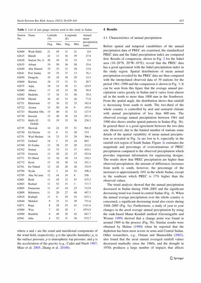
where u and v are the zonal and meridional components of

the wind field, respectively; q is the specific humidity; ps is

the surface pressure; p is atmospheric top pressure; and g is

the acceleration of the gravity (e.g., Cadet and Nnoli 1987;

Miao et al. 2005; Zhang et al. 2010b).

4 Results

4.1 Characteristics of annual precipitation

Before spatial and temporal variabilities of the annual

precipitation data of PREC are examined, the standardized

PREC data and the Sahel precipitation index are compared

first. Results of comparison, shown in Fig. 2 for the Sahel

area (10–20�N, 20�W–10�E), reveal that the PREC data

has a good agreement with the Sahel precipitation index in

the study region. Spatial distributions of mean annual

precipitation revealed by the PREC data are then compared

with the interpolated observed data of 39 stations for the

period 1961–1990 and the comparison is shown in Fig. 3. It

can be seen from this figure that the average annual pre-

cipitation varies greatly in Sudan and it varies from almost

nil in the north to more than 1000 mm in the Southwest.

From the spatial angle, the distribution shows that rainfall

is decreasing from south to north. The two-third of the

whole country is controlled by arid and semiarid climate

with annual precipitation of less than 600 mm. The

observed average annual precipitation between 1961 and

1990 also shows similar spatial patterns in Sudan (Fig. 3b).

In general there is a good agreement between the two data

sets. However, due to the limited number of stations some

details of the spatial variability of mean annual precipita-

tion as revealed in Fig. 3a are lost in b, especially in the

rainfall rich region of South Sudan. Figure 3c estimates the

magnitude and percentage of overestimations of PREC

precipitation compared to the observed precipitation which

provides important information for engineering designs.

The results show that PREC precipitation are higher than

observed precipitation, the amount of differences increases

from north to south, however, the percentage of the

increases is approximately 10% in the whole Sudan, except

in the southeast which PREC is 17% higher than the

observed values.

The trend analysis showed that the annual precipitation

decreased in Sudan during 1948–2005 and the significant

decreasing trend was found in central Sudan (Fig. 4). When

the annual average precipitation over the whole country is

concerned, a significant decreasing trend also exists during

1948–2005 (Fig. 5a). Furthermore, a study of year to year

changes in the areal average annual precipitation by using

the rank-based Mann–Kendall method (Gerstengarbe and

Werner 1999) showed that a change point was found in

around 1969 in the process (Fig. 5b). Similar results were

obtained by Hulme (1990) when he reported that the

depletion has been most severe in semi-arid Central Sudan.

Other researchers, e.g., Osman and Shamseldin (2002),

also found that the areal annual averaged rainfall values

decreased markedly since the 1960s, and the drought in

1970s produces a large number of impacts that affects

Table 1 List of rain gauge stations used in this study in Sudan

Station

No.

Name Latitude

(N)

Longitude

(E)

Annual

mean

precipitation

(mm)Deg. Min. Deg. Min.

62600 Wadi Halfa 21 49 31 21 0.6

62615 Halaib 22 13 36 39 27.8

62620 Station No. 6 20 45 32 33 5.9

62635 Arbaat 19 50 36 58 35.6

62640 Abu Hamed 19 32 33 20 12.6

62641 Port Sudan 19 35 37 13 76.1

62650 Dongola 19 10 30 29 12.3

62660 Karima 18 33 31 51 20.7

62675 Aqiq 18 14 38 11 124.9

62680 Atbara 17 42 33 58 59.9

62682 Hudeiba 17 34 33 56 39.4

62700 Shendi 16 42 33 26 77.6

62721 Khartoum 15 36 32 33 162.4

62722 Aroma 15 50 36 9 193.6

62723 Shambat Obs. 15 40 32 32 127.5

62730 Kassala 15 28 36 24 251.2

62733 Halfa El

Gedida

15 19 35 36 238.3

62735 Showak 14 24 35 51 501.9

62750 Ed Dueim 14 0 32 20 274

62751 Wad Medani 14 23 33 29 306.4

62752 Gedaref 14 2 35 24 603

62760 El Fasher 13 38 25 20 212.6

62762 Sennar 13 33 33 37 410.1

62770 Geneina 13 29 22 27 523.8

62771 El Obeid 13 10 30 14 318.1

62772 Kosti 13 10 30 14 351.1

62781 En Nahud 12 42 28 26 335.9

62790 Nyala 12 3 24 53 398.3

62795 Abu Na’ama 12 44 34 8 556

62801 Renk 11 45 32 47 475.2

62803 Rashad 11 52 31 3 717.7

62805 Damazine 11 47 34 23 712.9

62809 Babanusa 11 20 27 40 497.3

62810 Kadugli 11 0 29 43 633.1

62840 Malakal 9 33 31 39 731.6

62871 Raga 8 28 25 41 1141.6

62880 Wau 7 42 28 1 1074.5

62900 Rumbek 6 48 29 42 847.7

62941 Juba 4 52 31 36 972.7

Stoch Environ Res Risk Assess (2012) 26:429–441 433

123

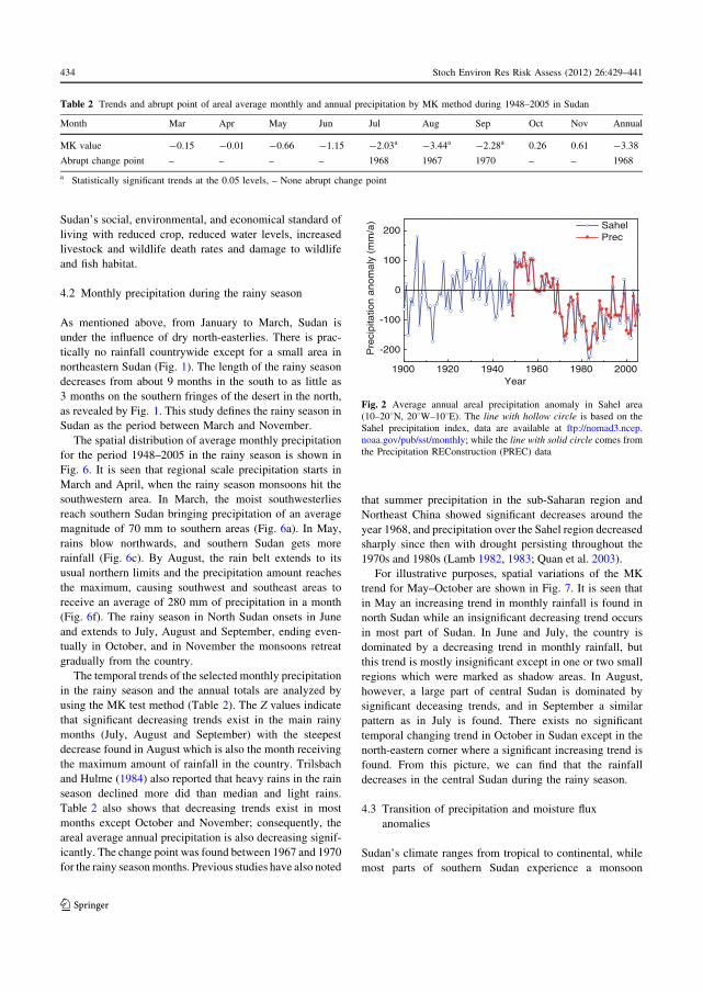
Sudan’s social, environmental, and economical standard of

living with reduced crop, reduced water levels, increased

livestock and wildlife death rates and damage to wildlife

and fish habitat.

4.2 Monthly precipitation during the rainy season

As mentioned above, from January to March, Sudan is

under the influence of dry north-easterlies. There is prac-

tically no rainfall countrywide except for a small area in

northeastern Sudan (Fig. 1). The length of the rainy season

decreases from about 9 months in the south to as little as

3 months on the southern fringes of the desert in the north,

as revealed by Fig. 1. This study defines the rainy season in

Sudan as the period between March and November.

The spatial distribution of average monthly precipitation

for the period 1948–2005 in the rainy season is shown in

Fig. 6. It is seen that regional scale precipitation starts in

March and April, when the rainy season monsoons hit the

southwestern area. In March, the moist southwesterlies

reach southern Sudan bringing precipitation of an average

magnitude of 70 mm to southern areas (Fig. 6a). In May,

rains blow northwards, and southern Sudan gets more

rainfall (Fig. 6c). By August, the rain belt extends to its

usual northern limits and the precipitation amount reaches

the maximum, causing southwest and southeast areas to

receive an average of 280 mm of precipitation in a month

(Fig. 6f). The rainy season in North Sudan onsets in June

and extends to July, August and September, ending even-

tually in October, and in November the monsoons retreat

gradually from the country.

The temporal trends of the selected monthly precipitation

in the rainy season and the annual totals are analyzed by

using the MK test method (Table 2). The Z values indicate

that significant decreasing trends exist in the main rainy

months (July, August and September) with the steepest

decrease found in August which is also the month receiving

the maximum amount of rainfall in the country. Trilsbach

and Hulme (1984) also reported that heavy rains in the rain

season declined more did than median and light rains.

Table 2 also shows that decreasing trends exist in most

months except October and November; consequently, the

areal average annual precipitation is also decreasing signif-

icantly. The change point was found between 1967 and 1970

for the rainy seasonmonths. Previous studies have also noted

that summer precipitation in the sub-Saharan region and

Northeast China showed significant decreases around the

year 1968, and precipitation over the Sahel region decreased

sharply since then with drought persisting throughout the

1970s and 1980s (Lamb 1982, 1983; Quan et al. 2003).

For illustrative purposes, spatial variations of the MK

trend for May–October are shown in Fig. 7. It is seen that

in May an increasing trend in monthly rainfall is found in

north Sudan while an insignificant decreasing trend occurs

in most part of Sudan. In June and July, the country is

dominated by a decreasing trend in monthly rainfall, but

this trend is mostly insignificant except in one or two small

regions which were marked as shadow areas. In August,

however, a large part of central Sudan is dominated by

significant deceasing trends, and in September a similar

pattern as in July is found. There exists no significant

temporal changing trend in October in Sudan except in the

north-eastern corner where a significant increasing trend is

found. From this picture, we can find that the rainfall

decreases in the central Sudan during the rainy season.

4.3 Transition of precipitation and moisture flux

anomalies

Sudan’s climate ranges from tropical to continental, while

most parts of southern Sudan experience a monsoon

Table 2 Trends and abrupt point of areal average monthly and annual precipitation by MK method during 1948–2005 in Sudan

Month Mar Apr May Jun Jul Aug Sep Oct Nov Annual

MK value -0.15 -0.01 -0.66 -1.15 -2.03a -3.44a -2.28a 0.26 0.61 -3.38

Abrupt change point – – – – 1968 1967 1970 – – 1968

a Statistically significant trends at the 0.05 levels, – None abrupt change point

1900 1920 1940 1960 1980 2000

-200

-100

0

100

200

Pre

cip

itatio

n a

no

ma

ly (

mm

/a)

Year

Sahel Prec

Fig. 2 Average annual areal precipitation anomaly in Sahel area

(10–208N, 208W–108E). The line with hollow circle is based on the

Sahel precipitation index, data are available at ftp://nomad3.ncep.

noaa.gov/pub/sst/monthly; while the line with solid circle comes from

the Precipitation REConstruction (PREC) data

434 Stoch Environ Res Risk Assess (2012) 26:429–441

123

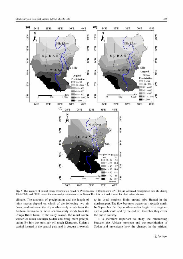
climate. The amounts of precipitation and the length of

rainy season depend on which of the following two air

flows predominates: the dry northeasterly winds from the

Arabian Peninsula or moist southwesterly winds from the

Congo River basin. In the rainy season, the moist south-

westerlies reach southern Sudan and bring more precipi-

tation. By July the moist air will reach Khartoum, Sudan’s

capital located in the central part, and in August it extends

to its usual northern limits around Abu Hamad in the

northern part. The flow becomes weaker as it spreads north.

In September the dry northeasterlies begin to strengthen

and to push south and by the end of December they cover

the entire country.

It is therefore important to study the relationship

between the African monsoon and the precipitation of

Sudan and investigate how the changes in the African

Fig. 3 The average of annual mean precipitation based on Precipitation REConstruction (PREC) (a), observed precipitation data (b) during1961–1990, and PREC minus the observed precipitation (c) in Sudan The dots in b and c stand for observation stations

Stoch Environ Res Risk Assess (2012) 26:429–441 435

123

monsoon have influenced the amount of precipitation

during the rainy season. It is also desirable to explore how

the African monsoon has changed and whether this change

is one of the main causes for the rainfall decrease and the

abrupt change in annual and monthly precipitation found

around 1968. Therefore, we analyzed the variability of

atmospheric moisture content and moisture flux in the past

decades and the average moisture flux anomalies to explain

the transition of precipitation in Sudan. From Fig. 8, it is

found that the whole layer of moisture content significantly

has decreased in central Sudan in summer since the late

1960s which might be related to the decline in precipitation

in central Sudan. The spatial distribution of temporal linear

trend of the atmospheric moisture flux in 1948–2005 in

Africa is shown in Fig. 9. It can be seen that the whole

layer of moisture flux in summer (JJA) during 1948–2005

decreased significantly in the central part of Africa

including Sudan. The significant negative trends of zonal

and meridional moisture flux found in Sudan indicated that

there was a weak western and southern moisture flux,

respectively. Figure 10 shows the spatial distribution of

summer moisture flux anomalies during 1970–2005, when

compared to that during 1948–1969. It is seen that there

was an obvious northeastern moisture flux in Sudan. The

northeasterly wind tendency in Sudan indicated that there

was a weak summer monsoon since the late 1960s, and the

weak summer monsoon limited the northward propagation

of moisture to North Sudan. As a result, precipitation

decreases significantly, especially in central Sudan. This

observation is in line with changes in precipitation in

Sudan, showing a close agreement between moisture flux

alterations and changes in precipitation. The changes in

African monsoon in the late 1960s make the circulation and

precipitation change. The decades of the 1970s and 1980s

saw the southwesterlies frequently fail, with disastrous

results for the Sudanese people and economy.

5 Discussions

The decrease in precipitation in rainy season has led to

more severe and longer-lasting droughts in Sudan.

Increasing drought frequency has the potential to affect

land-based natural and managed ecosystems, coastal sys-

tems, and both freshwater quality and quantity (Alvi 1994;

Janowiak 1988; Nicholson et al. 2000). The current study

Fig. 4 The MK trends in annual precipitation in Sudan. The values of

contour lines depict the test statistics Z values of MK test. Solid linesindicate increasing regions and dashed lines indicate decreasing

regions, and gray regions indicate the trend is statistically significant

at the 5% significance level

(a)

(b)

Fig. 5 a The linear trend of areal average annual precipitation in

Sudan (P-values show the significance level and when the P-value is

smaller than 0.05 meaning that the trend is statistically significant at

5% significance level); b the turning point detected by using MK

method. The time series has a downward trend if UF\ 0 and an

increasing trend if UF[ 0. If the UF value is greater than the critical

values (the two dashed lines), then this upward or downward trend is

significant at 5% significance level. When the UF and UB curves

intersect at a certain time, the intersection point denotes the jumping

time

436 Stoch Environ Res Risk Assess (2012) 26:429–441

123

reveals the annual and monthly changing characteristics of

precipitation during 1948–2005 in Sudan. The annual

precipitation has a significant decreasing trend in central

Sudan, which is particularly caused by the decrease in the

amount of rains in July, August and September. The

decreasing trend in precipitation in Sudan, particularly

after mid-1960s, is in agreement with regional precipitation

changes as reported in earlier studies. For example, Eltahir

(1988) and Long et al. (2000) found the annual rainfall

amounts in the entire region of central and western Africa

decreased since the late 1960s. The mechanisms of

droughts in Sudan are complex and many studies have been

made to examine the causes of droughts. However, the

cause of the Sahel drought remains elusive (Nicholson

S U D A N

While Nile

Blue Nile

Nile River

(a) March

S U D A N

While Nile

Blue Nile

Nile River

(b) April

S U D A N

While Nile

Blue Nile

Nile River

(c) May

S U D A N

While Nile

Blue Nile

Nile River

(d) June

S U D A N

While Nile

Blue Nile

Nile River

(e) July

S U D A N

While Nile

Blue Nile

Nile River

(f) August

S U D A N

While Nile

Blue Nile

Nile River

(g) September

S U D A N

While Nile

Blue Nile

Nile River

(h) October

S U D A N

While Nile

Blue Nile

Nile River

(i) November

0 10 30 50 100 150 200 250 300mm

Fig. 6 The monthly average precipitation in rainy season in Sudan averaged over the period 1948–2005

Stoch Environ Res Risk Assess (2012) 26:429–441 437

123

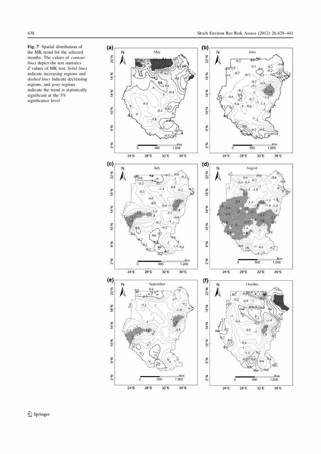
Fig. 7 Spatial distribution of

the MK trend for the selected

months. The values of contourlines depict the test statistics

Z values of MK test. Solid linesindicate increasing regions and

dashed lines indicate decreasingregions, and gray regions

indicate the trend is statistically

significant at the 5%

significance level

438 Stoch Environ Res Risk Assess (2012) 26:429–441

123

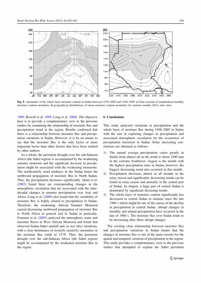
1989; Rowell et al. 1995; Long et al. 2000). The objective

here is to provide a complementary view to the previous

studies by examining the relationship of moisture flux and

precipitation trend in the region. Results confirmed that

there is a relationship between moisture flux and precipi-

tation variations in Sudan. However, it is by no means to

say that the moisture flux is the only factor or more

important factor than other factors that have been studied

by other authors.

As a whole, the persistent drought over the sub-Saharan

Africa (the Sahel region) is accompanied by the weakening

summer monsoon and the significant decrease in precipi-

tation might be associated with the weakening monsoons.

The northeasterly wind tendency in the Sudan limits the

northward propagation of moisture flux to North Sudan.

Thus, the precipitation decreases significantly. Quan et al.

(2003) found there are corresponding changes in the

atmospheric circulation that are associated with the inter-

decadal changes in summer precipitation over Asia and

Africa. Long et al. (2000) also found that the variability of

moisture flux is highly related to precipitation in Sudan.

Therefore, the weakening African Summer Monsoon

caused decreasing northward propagation of moisture flux

to North Africa in general and in Sudan in particular.

Fontaine et al. (2003) analyzed the atmospheric water and

moisture fluxes in West African Monsoon and found that

observed Sudan-Sahel rainfall and, in wet (dry) situations,

with a clear dominance of westerly (easterly) anomalies in

the moisture flux south of 15�N. Thus, the persistent

drought over the sub-Saharan Africa (the Sahel region)

might be accompanied by the weakened moisture flux in

the region.

6 Conclusions

This study analyzed variations in precipitation and the

whole layer of moisture flux during 1948–2005 in Sudan

with the aim of exploring changes in precipitation and

associated atmospheric circulation for the occurrence of

precipitation transition in Sudan. Some interesting con-

clusions are obtained as follows:

1) The annual average precipitation varies greatly in

Sudan from almost nil in the north to about 1500 mm

in the extreme Southwest. August is the month with

the highest precipitation rates in Sudan; however, the

biggest decreasing trend also occurred in this month.

2) Precipitation decreases almost in all months in the

rainy season and significantly decreasing trends can be

found in rainy season and annually in the central part

of Sudan. In August, a large part of central Sudan is

dominated by significant deceasing trends.

3) The whole layer of moisture content significantly has

decreased in central Sudan in summer since the late

1960 s which might be one of the causes of the decline

in precipitation in central Sudan. Abrupt changes in

monthly and annual precipitation have occurred in the

late of 1960 s. The moisture flux over Sudan tends to

be decreasing after these abrupt changes.

The existing clear relationship between moisture flux

and precipitation variations in Sudan means that the

changes in moisture flux is one of the main reasons for the

spatial and temporal variation of precipitation in the region.

This study provides a complementary view to the previous

studies that attempted to explain the Sahel persistent

(a) (b)

Fig. 8 Anomalies of the whole layer moisture content in Sudan between 1970–2005 and 1948–1969. a Time sections of standardized monthly

moisture content anomalies; b geographical distributions of mean moisture content anomalies for summer months (JJA), unit: mm)

Stoch Environ Res Risk Assess (2012) 26:429–441 439

123

drought in terms of general circulation features, sea surface

temperatures, land surface feedback mechanisms, and

teleconnected, spatiotemporal rainfall patterns.

Acknowledgments This work is financially supported by The

Research Council of Norway (RCN) with project number 171783

(FRIMUF), the Chinese ‘‘985 Project’’ (Grant no. 37000-3171315) and

the Program of Introducing Talents of Discipline to Universities—the

111 Project of Hohai University. We would like to thank Prof. Dr

Mingyue Chen who provided us the global Precipitation RECon-

struction (PREC) data, and the data download website can be found in

the National Oceanic and Atmospheric Administration (NOAA) Cli-

mate Prediction Center: ftp.cpc.ncep.noaa.gov/precip/50yr/.

Open Access This article is distributed under the terms of the

Creative Commons Attribution Noncommercial License which per-

mits any noncommercial use, distribution, and reproduction in any

medium, provided the original author(s) and source are credited.

References

Alvi SH (1994) Climate changes, desertification and the Republic of

Sudan. GeoJournal 33(4):393–399

Cadet DL, Nnoli NO (1987) Water vapour transport over Africa and

the Atlantic Ocean during summer 1979. Quart J Royal Meteorol

Soc 113(476):581–602

Camberlin P (1995) June–September rainfall in north-eastern Africa

and atmospheric signals over the Tropics: a zonal perspective.

Int J Climatol 15:773–783

Chen MY, Xie P, Janowiak JE, Arkin PA (2002) Global land

precipiation: a 50-yr monthly analysis based on gauge observa-

tions. J Hydrometeorol 3:249–266

Cook KH, Vizy EK (2006) Coupled model simulations of the West

African monsoon system: twentieth and twenty first century

simulations. J Clim 19:3681–3703

Eltahir EAB (1988) Testing trends in annual rainfall in central and

western Sudan. Sudan Eng Soc J 30:37–50

Eltahir EAB (1992) Drought frequency analysis of annual rainfall

series in central and western Sudan. J Hydrol Sci 37:185–199

Fontaine B, Roucou P, Trzaska S (2003) Atmospheric water cycle and

moisture fluxes in the West African monsoon: mean annual

cycles and relationship using NCEP/NCAR reanalysis. Geophys.

Res. Lett., 30(3):1117. doi:10.1029/2002GL015834

Gerstengarbe FW, Werner PC (1999) Estimation of the beginning and

end of recurrent events within a climate regime. Climate

Research 11:97–107

Hulme M (1987) Secular changes in wet season structure in central

Sudan. J Arid Environ 13:31–46

Hulme M (1990) The changing rainfall resources of Sudan. Trans Inst

Brit Geogr 15(1):21–34

Hulme M, Tosdevin N (1989) The tropical easterly jet and Sudan

rainfall: a review. Theor Appl Climatol 39:179–187

Janowiak JE (1988) An investigation of interannual rainfall variabil-

ity in Africa. J Clim 1:240–255

Janowiak JE, Gruber A, Kondragunta CR et al (1998) A comparison

of the NCEP-NCAR reanalysis precipitation and the GPCP

raingauge-satellite combined dataset with observational error

considerations. J Clim 11:2960–2979

Kendall MG (1975) Rank correlation methods. Griffin, London

Lamb PJ (1978a) Large-scale tropical Atlantic surface circulation

patterns associated with Subsaharan weather anomalies. Tellus

30:240–251

(b)

(a)

Fig. 9 Spatial distributionof linear trends inwhole layermoisture flux in

summer (JJA) during 1948–2005 at zonal moisture flux (a) and meridi-

onal moisture flux (b) in Africa. The contours indicate the correlation

coefficient between time and the moisture flux, for which values large

than±0.3 is statistically significant at the 5% significant level

Fig. 10 Spatial distribution of the summer (JJA) atmospheric mois-

ture flux anomalies between 1970–2005 and 1948–1969 (shadedregions indicate[20 kg/m s, unit: kg/m s)

440 Stoch Environ Res Risk Assess (2012) 26:429–441

123

Lamb PJ (1978b) Case studies of tropical Atlantic surface circulation

patterns during recent Subsaharan weather anomalies: 1967 and

1968. Mon Wea Rev 106:482–491

Lamb PJ (1982) Persistence of sub-Sahara drought. Nature 299:46–47

Lamb PJ (1983) Sub-Sahara rainfall update for 1982: continued

drought. Int J Climatol 3(4):419–422

Long M, Dara E, Sharon EN (2000) Interannual variability in rainfall,

water vapor flux, and vertical motion over West Africa. J Clim

13:3827–3841

Mann HB (1945) Nonparametric tests against trend. Econometrica

13:245–259

Miao QJ, Xu XD, Zhang SY (2005) Whole layer water vapor budget

of Yangtze River valley and moisture flux components transform

in the key areas of the plateau. Acta Meteorol Sinica 63:93–99

Nicholson SE (1986) The spatial coherence of African rainfall

anomalies: interhemispheric teleconnections. J Climate Appl

Meteorol 25(10):1365–1381

Nicholson SE (1989) African drought: characteristics, causal theories

and global teleconnections. In: Berger A, Dickinson RE and

Kidson JW (eds.) Understanding climate change. American

geophysical union geophysical monograph 52:79–100

Nicholson SE, Some B, Kone B (2000) An analysis of recent rainfall

conditions in West Africa, including the rainy seasons of the

1997 El Nino and the 1998 La Nina Years. J Clim 13:2628–2640

Osman and Hastenrath (1969) On the synoptic climatology of the

summer rainfall over central Sudan. Arch Met Geoph Biokl Ser

B 17:297–324

Osman YZ, Shamseldin AY (2002) Qualitative Rainfall prediction

models for central and southern Sudan using El Nino Southern

Oscillation and Indian sea surface temperature indices. Int.

J. Climatology 22:1861–1878

Palmer TN (1986) Influence of the Atlantic, Pacific and Indian

Oceans on Sahel rainfall. Nature 322:251–253

Poccard I, Janicot S, Camberlin P (2000) Comparison of rainfall

structures between NCEP/NCAR reanalysis and observed data

over Tropical Africa. Climate Dyn 16:897–915

Prueger JH, Kustas WP, Hipps LE, Hatfield JL (2004) Aerodynamic

parameters and sensible heat flux estimates for a semi-arid

ecosystem. J Arid Environ 57:87–100

Quan XW, Diaz HF, Fu CB (2003) Interdecadal change in the Asia–

Africa summer monsoon and its associated changes in global

atmospheric circulation. Global Planet Change 37(3–4):171–188

Rowell DP, Folland CK, Maskell K, Ward N (1995) Variability of

summer rainfall over tropical North Africa (1906–92): Obser-

vations and modelling. Quart J Roy Meteor Soc 121:669–704

Shi N, Chen LW, Xia DD (2002a) A preliminary study on the global

land annual precipitation associated with ENSO during

1948–2000. Advan Atmosph Sci 19(6):993–1003

Shi N, Chen LW, Lin ZM (2002b) The relationship between global

precipitation and local monsoon precipitation. Meteorolo Sci

Technol 30(2):73–79 (in Chinese)

Shi N, Chen LW, Fen GL et al (2004) Climate characters and changes

in global precipitation field from 1920 to 2000. Plateau Meteorol

23(4):436–443 (in Chinese)

Sneyers R (1990) On statistical analysis of series of observations.

WMO Tech Note, WMO:143

Trilsbach A, Hulme M (1984) Recent rainfall changes in central

Sudan and their physical and human implications. Trans Inst Brit

Geogr 9:280–298

Von Storch VH (1995) Misuses of statistical analysis is climate

research. In: von Storch VH, Navarra A (eds) Analysis of climate

variability: applications of statistical techniques. Springer-Ver-

lag, Berlin, pp 11–26

Walsh RPD, Hulme M, Campbell MD (1988) Recent rainfall changes

and their impact on hydrology and water supply in the semi-arid

zone of the Sudan. Geog. Jour 154(2):181–198

WMO (1966) Climate change: report of a working group of the

commission for climatology. WMO Tech:79

Xu C-Y (2001) Statistical analysis of a conceptual water balance

model, methodology and case study. Water Res Manag 15:75–92

Yue S, Wang CY (2002a) Applicability of prewhitening to eliminate

the influence of serial correlation on the Mann–Kendall test.

Water Resour Res 38(6):1068

Yue S, Wang CY (2002b) Discussion: a study of variability of annual

river flow of the southern African region. Hydrol Sci

47(6):983–989

Yue S, Pilon P, Cavadias G (2002) Power of the Mann–Kendall test

and the Spearman’s rho test for detecting monotonic trends in

hydrological time series. J Hydrol 259:254–271

Zhang Q, Xu C-Y, Zhang Z, Chen YD, Liu C-L (2009) Spatial and

temporal variability of precipitation during 1951–2005 over

China. Theor Appl Climatol 95:53–68

Zhang Q, Xu C-Y, Tao H, Jiang T, Chen YD (2010a) Climate changes

and their impacts on water resources in the arid regions: a case

study of the Tarim River basin, China. Stoch Env Res Risk

Assess 24:349–358

Zhang ZX, Tao H, Zhang Q et al (2010b) Moisture budget variations

in the Yangtze River Basin, China, and possible associations

with large-scale circulation. Stoch Environ Res Risk Assess

24(5):579–589

Zhou J, Xue YF, Liu XF (1998) The source/sink distribution of water

vapor with its transfer in Asian monsoon region in August, 1994.

J Trop Meteorol 14(1):91–96

Stoch Environ Res Risk Assess (2012) 26:429–441 441

123