Embed Size (px)
Citation preview
A Central Limit Theorem for Realised Powerand Bipower Variations of ContinuousSemimartingales
Ole E. BARNDORFF–NIELSEN1, Svend Erik GRAVERSEN2,Jean JACOD3, Mark PODOLSKIJ4?, and Neil SHEPHARD5
1 Dept. of Mathematical Sciences, University of Aarhus, Ny Munkegade, DK–8000Aarhus C, Denmark, (e-mail: [email protected])
2 Dept. of Mathematical Sciences, University of Aarhus, Ny Munkegade, DK–8000Aarhus C, Denmark, (e-mail:[email protected])
3 Laboratoire de Probabilites et Modeles Aleatoires (CNRS UMR 7599) UniversiteP. et M. Curie, 4 Place Jussieu, 75 252 - Paris Cedex, France.(e-mail: [email protected])
4 Ruhr University of Bochum, Dept. of Probability and Statistics,Universitatstrasse 150, 44801 Bochum, Germany, (e-mail:[email protected])
5 Nuffield College, Oxford OX1 1NF, UK, (e-mail: [email protected])
Abstract Consider a semimartingale of the form Yt = Y0 +R t
0asds +
R t
0σs− dWs,
where a is a locally bounded predictable process and σ (the “volatility”) is anadapted right–continuous process with left limits and W is a Brownian motion. We
consider the realised bipower variation process V (Y ; r, s)nt = n
r+s2 −1P[nt]
i=1 |Y in−
Y i−1n|r|Y i+1
n−Y i
n|s, where r and s are nonnegative reals with r+s > 0. We prove that
V (Y ; r, s)nt converges locally uniformly in time, in probability, to a limiting process
V (Y ; r, s)t (the ”bipower variation process”). If further σ is a possibly discontinuoussemimartingale driven by a Brownian motion which may be correlated with W andby a Poisson random measure, we prove a central limit theorem, in the sense that√
n (V (Y ; r, s)n − V (Y ; r, s)) converges in law to a process which is the stochasticintegral with respect to some other Brownian motion W ′, which is independent ofthe driving terms of Y and σ. We also provide a multivariate version of these results,and a version in which the absolute powers are replaced by smooth enough functions.
Key words: Central limit theorem, quadratic variation, bipower variation,
Mathematics Subject Classification (2000): 60F17, 60G44
? This author has been partially supported by the DYNSTOCH Research TrainingNetwork. The financial support of the Deutsche Forschungsgemeinschaft (SFB475, ”Reduction of complexity in multivariate data structures”) is gratefully ac-knowledged.
2 O. E. Barndorff–Nielsen et al
1 Introduction
For a wide class of real–valued processes Y , including all semimartingales, the“approximate (or, realised) quadratic variation processes”
V (Y ; 2)nt =[nt]∑i=1
(Y in− Y i−1
n)2, (1.1)
where [x] denotes the integer part of x ∈ R+, converge in probability, asn → ∞ and for all t ≥ 0, towards the quadratic variation process V (Y ; 2)t(usually denoted by [Y, Y ]t).
This fact is basic in the ”general theory of processes” and is also usedin a large variety of more concrete problems, and in particular for the sta-tistical analysis of the process Y when it is observed at the discrete timesi/n : i = 0, 1, . . . (sometimes V (Y ; 2)nt is called the “realised” quadraticvariation, since it is explicitly calculable on the basis of the observations).In that context, in addition to the convergence in probability one is inter-ested in the associated CLT (Central Limit Theorem), which says that the√n (V (Y ; 2)nt − V (Y ; 2)t)’s converge in law, as processes, to a non–trivial lim-
iting process. Of course, for the CLT to hold we need suitable assumptions onY . This type of tool has been used very widely in the study of the statisticsof processes in the past twenty years. References include, for example, thereview paper [10] in the statistics of processes and [1], [2], [3], [6] in financialeconometrics. [2] provides a review of the literature in econometrics on thistopic.
Now, when Y describes some stock price, with a stochastic volatility possi-bly having jumps, a whole new class of processes extending the quadratic vari-ation has been recently introduced, and named “bipower variation processes”:let r, s be nonnegative numbers. The realised bipower variation process of order(r, s) is the increasing processes defined as:
V (Y ; r, s)nt = nr+s2 −1
[nt]∑i=1
|Y in− Y i−1
n|r |Y i+1
n− Y i
n|s, (1.2)
with the convention 00 = 1. Clearly V (Y ; 2)n = V (Y ; 2, 0)n. The bipowervariation process of order (r, s) for Y , denoted by V (Y ; r, s)t, is the limit inprobability, if it exists for all t ≥ 0, of V (Y ; r, s)nt . It has been introducedin [4] and [5], where it is shown that the bipower variation processes existfor all nonnegative indices r, s as soon as Y is a continuous semimartingaleof “Ito type” with smooth enough coefficients. These papers also contain aversion of the associated CLT under somewhat restrictive assumptions andwhen r = s = 1.
The aim of this paper is mainly to investigate the CLT, and more preciselyto give weaker conditions on Y which ensure that it holds and which cover
CLT for bipower variations 3
most concrete situations of interest, and also to precisely describe the limitingprocess. We prove the existence of the bipower variation process for a wideclass of continuous semimartingales (extending the results of [4] and [5]). Weestablish the CLT in a slightly more restricted setting. The restriction is thatthe volatility of Y (that is, the coefficient in front of the driving Wiener processfor Y ) is a semimartingale driven by a Levy process, or more generally by aWiener process (possibly correlated with the one driving Y ) and a Poissonrandom measure.
We also investigate the multidimensional case, when Y = (Y j)1≤j≤d is d–dimensional. It is then natural to replace (1.2) by the realised “cross–bipowervariation processes”:
V (Y j , Y k; r, s)nt = nr+s2 −1
[nt]∑i=1
|Y jin
− Y ji−1n
|r |Y ki+1n
− Y kin|s. (1.3)
We state the results in Section 2, and the proofs are given in the othersections. The reader will notice that we replace the powers like |Y i
n− Y i−1
n|r
in (1.2) by an expression of the form g(√n(Y i
n−Y i−1
n)) for a suitable function
g: this can prove useful for some applications, and it is indeed a simplificationrather than a complication for the proof itself. Written in this way, our resultsalso extend some of the results of Becker in [7], and of the unpublished paper[8].
It is also worth observing that, apart from the notational complexity, theproofs when r > 0 and s > 0 are not really more difficult than when r > 0and s = 0, that is when we have only one power in (1.2). That means that,obviously, the same types of results would hold for the ”realised multipowervariation processes” which are defined by
V (Y j1 , . . . , Y jN ; r1, . . . , rN )nt
= nr1+...+rN
2 −1
[nt]∑i=1
|Y j1in
− Y j1i−1n
|r1 . . . |Y jNi+N−1n
− Y jNi+N−2n
|rN , (1.4)
for any choice of ri ≥ 0 and any fixed N . We do not prove those more generalresults here, but simply state the results.
2 Statement of results
We start with a filtered space (Ω,F , (F t)t≥0,P), on which are defined variousprocesses, possibly multidimensional: so we systematically use matrix andproduct–matrices notations. The transpose is denoted by ?, all norms aredenoted by ‖.‖. We denote by Md,d′ the set of all d × d′–matrices, and byMd,d′,d′′ the set of all arrays of size d × d′ × d′′, and so on. For any processX we write ∆n
i X = Xi/n −X(i−1)/n.
4 O. E. Barndorff–Nielsen et al
Our basic process is a continuous d–dimensional semimartingale Y =(Y i)1≤i≤d. We are interested in the asymptotic behavior of all finite fami-lies of processes of type (1.3), that is for all j, k ∈ 1, . . . , d and all finitefamilies of pairs (r, s). So in order to simplify notation (which will neverthe-less remain quite complicated, sorry for that !), we introduce the followingprocesses:
Xn(g, h)t =1n
[nt]∑i=1
g(√n ∆n
i Y )h(√n ∆n
i+1Y ), (2.1)
where g and h are two maps on Rd, taking vakues in Md1,d2 and Md2,d3
respectively. So Xn(g, h)t takes its values in Md1,d3 . Note that, letting
fj,r(x) = |xj |r, (2.2)
we have V (Y j , Y k; r, s)n = Xn(fj,r, fk,s), and any finite family of processeslike in (1.3) is a process of the type (2.1) with the components of g and hbeing the various fj,r.
2.1 Convergence in probability
We start with the convergence in probability of the processes Xn(g, h). Weneed the following structural assumption on Y :
Hypothesis (H): We have
Yt = Y0 +∫ t
0
asds+∫ t
0
σs− dWs, (2.3)
where W is a standard d′–dimensional BM, a is predictable Rd–valued locallybounded, and σ is Md,d′–valued cadlag.
Below ρΣ denotes the normal law N (0, ΣΣ?
), and ρΣ(g) is the integral ofg w.r.t. ρΣ .
Theorem 2.1. Under (H) and when the functions g and h are continuouswith at most polynomial growth, we have
Xn(g, h)t → X(g, h)t :=∫ t
0
ρσs(g)ρσs
(h)ds, (2.4)
where the convergence is local uniform in time, and in probability.
If we apply this with the functions g = fj,r and h = fk,s, we get a resultof existence for the bipower variation processes. We denote by µr the rthabsolute moment of the law N (0, 1).
CLT for bipower variations 5
Theorem 2.2. Under (H), and if r, s ≥ 0, we have
V (Y j , Y k; r, s)nt → V (Y j , Y k; r, s)t := µrµs
∫ t
0
|σjju |r|σkku |s du, (2.5)
where the convergence is local uniform in time, and in probability.
This result is essentially taken from [4]. The assumption (H) could beweakened, of course, but probably not in any essential way. For instance thecadlag hypothesis on σ can be relaxed, but we need at least the functionsu 7→ |σjju |r to be Riemann–integrable, for all (or P–almost all) ω. The factthat the driving terms in (2.3) are t and Wt is closely related to the fact thatthe discretization in time has a constant step 1/n. If we replace (2.3) by
Yt = Y0 +∫ t
0
asdAs +∫ t
0
σs−dMs
where A is a continuous increasing process and M a continuous martingale,then a result like (2.5) can hold only for discretization along increasing se-quences of stopping times, related in some way to A and to the quadraticvariation of M . If further Y is discontinuous, this type of result cannot pos-sibly hold (with the normalizing factor n
r+s2 −1), as is easily seen when Y is
a simple discontinuous process like a Poisson process. As a matter of fact,this observation was the starting point of the papers [4] and [5] for intro-ducing bipower variations, in order to discriminate between continuous anddiscontinuous processes.
Finally, we state the multipower variation result: the processes of (1.4)converge (under (H)) towards
V (Y j1 , . . . , Y jN ; r1, . . . , rN )t = µr1 . . . µrN
∫ t
0
|σj1j1u |r1 . . . |σjN jNu |rN du.
(2.6)
2.2 The central limit theorem
For the CLT we need some additional structure on the volatility σ. A relativelysimple assumption is then:
Hypothesis (H0): We have (H) with
σt = σ0 +∫ t
0
a′sds+∫ t
0
σ′s−dWs +∫ t
0
vs−dZs, (2.7)
where Z is a d′′–dimensional Levy process on (Ω,F , (F t)t≥0,P), independentof W (and possibly with a non–vanishing continuous martingale part). Fur-thermore the processes σ′ and v, and a of (2.7), are adapted cadlag, with val-ues in Md,d′,d′ and Md,d′,d′′ and Md,d′ respectively, and a′ is Md,d′–valued,predictable and locally bounded.
6 O. E. Barndorff–Nielsen et al
This assumption is in fact not general enough for applications. Quite oftenthe natural ingredient in our model is the ”square” c = σσ∗ rather than σitself, and it is this c which satisfies an equation like (2.7). In this case the”square–root” σ of c does not usually satisfy a similar equation. This is whywe may replace (H0) by the following assumption:
Hypothesis (H1): We have (H) with
σt = σ0 +∫ t
0
a′sds+∫ t
0
σ′s−dWs +∫ t
0
vs−dVs +∫ t
0
∫E
ϕ w(s−, x)(µ− ν)(ds, dx) +∫ t
0
∫E
(w − ϕ w)(s−, x)µ(ds, dx). (2.8)
Here a′ and σ′ and v are like in (H0); V is a d′′–dimensional Wiener processindependent of W , with an arbitrary covariance structure; µ is a Poisson ran-dom measure on (0,∞)×E independent of W and V , with intensity measureν(dt, dx) = dtF (dx) and F is a σ–finite measure on the Polish space (E, E);ϕ is a continuous truncation function on Rdd′ (a function with compact sup-port, which coincides with the identity map on a neigbourhood of 0); finallyw(ω, s, x) is a map Ω × [0,∞) × E → Md,d′ which is Fs ⊗ E–measurablein (ω, x) for all s and cadlag in s, and such that for some sequence (Sk) ofstopping times increasing to +∞ we have:
supω∈Ω,s<Sk(ω)
‖w(ω, s, x)‖ ≤ ψk(x), where∫E
(1∧ψk(x)2) F (dx) <∞.
(2.9)
This hypothesis looks complicated, but it is usually simple to check. Theconditions on the coefficients imply in particular that all integrals in (2.8) arewell defined. It is weaker than (H0): indeed if (H0) holds, we also have (H1)with E = Rd′′ and V being the Wiener part of Z if it exists, and µ being therandom measure associated with the jumps of Z (so F is the Levy measure ofZ), and w(ω, t, x) = vt(ω)x (note that v is the same in (2.7) and in (2.8); theprocesses a′ in the two formulae are different, depending on the drift of Z).
We also sometimes need an additional assumption:
Hypothesis (H’): The process σσ? is everywhere invertible.
Set once more c = σσ∗. If the processes c and c− are invertible, (H1)holds if and only if the process c satisfies an equation like (2.8), with the sameassumptions on the coefficients. This is not longer true if we replace (H1) and(2.8) by (H0) and (2.7).
As for the functions g and h, we will suppose that their components satisfyone of the following assumptions, which we write for a real–valued functionf on Rd; if f is differentiable at x, we write ∇f(x) for the row matrix of itspartial derivatives:
CLT for bipower variations 7
Hypothesis (K): The function f is even (that is, f(−x) = f(x) for allx ∈ Rd) and continuously differentiable, with partial derivatives having atmost polynomial growth.
Hypothesis (K’): The function f is even, and continuously differentiable onthe complement Bc of a closed subset B ⊂ Rd and satisfies
‖y‖ ≤ 1 ⇒ |f(x+ y)− f(x)| ≤ C(1 + ‖x‖p) ‖y‖r (2.10)
for some constants C > 0, p ≥ 0 and r ∈ (0, 1]. Moreover:a) If r = 1 then B has Lebesgue measure 0.b) If r < 1 then B satisfies
for any positive definite d× d matrix C and anyN (0, C)–random vector U the distance d(U,B)from U to B has a density ψC on R+, such thatsupx∈R+,‖C‖+‖C−1‖≤A ψC(x) <∞ for all A <∞,
(2.11)
and we have
x ∈ Bc, ‖y‖ ≤ 1∧ d(x,B)
2⇒
‖∇f(x)‖ ≤ C(1+‖x‖p)d(x,B)1−r ,
‖∇f(x+ y)−∇f(x)‖ ≤ C(1+‖x‖p)‖y‖d(x,B)2−r .
(2.12)
The additional requirements when r < 1 above are not “optimal”, butthey accomodate the case where f equals fj,r, as defined in (2.2): this functionsatisfies (K) when r > 1, and (K’) when r ∈ (0, 1] (with the same r of course).When B is a finite union of hyperplanes it satisfies (2.11). Also, observe that(K) implies (K’) with r = 1 and B = ∅. For the concept of “stable convergencein law”, introduced by Renyi in [11], we refer to [9] for example; it is a kindof convergence which is a bit stronger than the ordinary convergence in law.
Theorem 2.3. Under (H1) (or (H0)) and either one the following assump-tions:
(i) all components of g and h satisfy (K),(ii) (H’) holds, and all components of g and h satisfy (K’),
the processes√n (Xn(g, h)−X(g, h)) converge stably in law towards the lim-
iting process U(g, h) given componentwise by
U(g, h)jkt =d1∑j′=1
d3∑k′=1
∫ t
0
α(σs, g, h)jk,j′k′ dW ′j′k′
s (2.13)
where
8 O. E. Barndorff–Nielsen et al∑d1l=1
∑d3m=1 α(Σ, g, h)jk,lmα(Σ, g, h)j
′k′,lm = A(Σ, g, h)jk,j′k′
and A(Σ, g, h)jk,j′k′ =
∑d2l,l′=1
(ρΣ(gjlgj
′l′)ρΣ(hlkhl′k′)
+ρΣ(gjl)ρΣ(hl′k′)ρΣ(gj
′l′hlk) + ρΣ(gj′l′)ρΣ(hlk)ρΣ(gjlhl
′k′)
−3ρΣ(gjl)ρΣ(gj′l′)ρΣ(hlk)ρΣ(hl
′k′)),
(2.14)
and W ′ is a d1d3–dimensional Wiener process which is defined on an extensionof the space (Ω,F , (F t)t≥0,P) and is independent of the σ–field F .
The first formula in (2.14) means that α is a square–root of the d1d3×d1d3–matrix A, which is symmetric semi–definite positive. Observe that the rightsides of (2.4) and (2.13) always make sense, due to the fact that t 7→ σt iscadlag and thus with all powers locally integrable w.r.t. Lebesgue measure.
Under (H) and if both g and h are even and continuous, the processes
Un(f, g)t =1√n
[nt]∑i=1
(g(√n ∆n
i Y )h(√n ∆n
i+1Y )
−E(g(√n ∆n
i Y )h(√n ∆n
i+1Y )|F i−1n
))
(2.15)
still converge stably in law to U(g, h) provided a and σ have some integra-bility properties in connection with the growth rate of g and h (so that theconditional expectations above are meaningful): see Theorem 5.1 below for aversion of this when a and σ are bounded. But such a CLT is probably oflittle practical use.
Remarks: For simplicity we state the remarks when all processes are 1–dimensional and when h(x) = 1.
1. When g is not even we still have a limiting process which is the processU(g, 1) plus a process which has a drift and an integral term w.r.t. W :for example if g(x) = x, then X(g, 1) = 0 and of course
√n Xn(g, h)t =
Y[nt]/n, so the limit is Y itself (in this case U(g, 1) = 0). For more details,see [8].
2. In view of the result on (2.15), when h = 1 the CLT is essentially equiva-lent to the convergence of
1√n
[nt]∑i=1
(E(g(
√n ∆n
i Y )|F i−1n
)− n
∫ in
i−1n
ρσu(g)du
)
to 0 (locally uniform in t). This in turn is implied by the convergence to0 of the following two processes:
CLT for bipower variations 9
1√n
[nt]∑i=1
(E(g(
√n ∆n
i Y )|F i−1n
)−E(g(√n σ i−1
n∆niW )|F i−1
n))
(2.16)
1√n
[nt]∑i=1
(ρσ i−1
n
(g)− n
∫ in
i−1n
ρσu(g)du
). (2.17)
3. For (2.17) we need some smoothness of σ: e.g. u 7→ σu is Holder withsome index > 1/2. Hypothesis (H1) is of this kind (although σ can havejumps, (2.8) sort of implies that it is ”Holder” of order 1/2 and furthersome compensation arises).
4. The differentiability of g is in fact used for the convergence of (2.16).Another natural idea would be to compare the transition densities of Yand W for small times, provided of course the former ones exist: thatallows to get the results for functions g and h which are only Borel–measurable, in Theorem 2.3 and in Theorem 2.1 as well, but it necessitatesquite stringent assumptions on Y (like a Markov structure, and non–degeneracy).
2.3 Applications to bipower variations
Let us now explain how the general CLT above writes for bipower variations.The most general form is given below, but for simplicity we first consider the1–dimensional case for Y , with a single bipower process.
Theorem 2.4. Let r, s ≥ 0 and assume that d = d′ = 1. Under (H1) andif either r, s ∈ 0 ∪ (1,∞) or (H’) holds, the processes (
√n (V (Y ; r, s)n −
V (Y ; r, s))) converge stably in law towards a limiting process U(r, s) of theform
U(r, s)t =√µ2rµ2s + 2µrµsµr+s − 3µ2
rµ2s
∫ t
0
|σu|r+s dW ′u, (2.18)
where W ′ is a Wiener process which is defined on an extension of the space(Ω,F , (F t)t≥0,P) and is independent of the σ–field F .
For the general case we consider simultaneously all cross–bipower varia-tions for any finite family of indices. We need some more notation: we de-note by µ(Σ; r, s; j, k) the expected value of |Uj |r|Uk|s when U = (Uj)1≤j≤dis an N (0, ΣΣ∗)–distributed random variable, and also by µ(Σ; r; j) the ex-pected value of |Uj |r (so µ(Σ; r; j) = µ(Σ; r, 0; j, k) for any k, and µ(Σ; r; j) =|Cjj |r/2µr, where C = ΣΣ∗).
Theorem 2.5. Let (rl, sl) be a family of nonnegative reals. Under (H1) andeither one of the following assumptions:
(i) rl, sl ∈ 0 ∪ (1,∞),(ii) (H’) and rl, sl ∈ [0,∞),
the L× d× d–dimensional processes
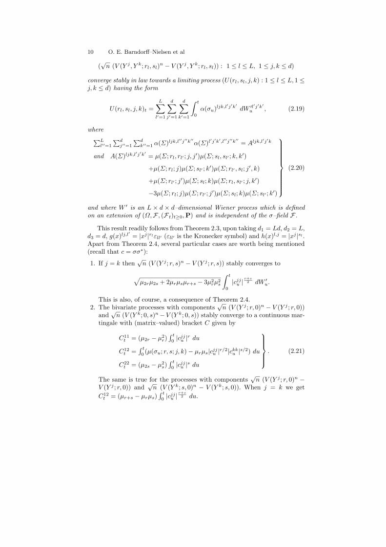
10 O. E. Barndorff–Nielsen et al
(√n (V (Y j , Y k; rl, sl)n − V (Y j , Y k; rl, sl)) : 1 ≤ l ≤ L, 1 ≤ j, k ≤ d)
converge stably in law towards a limiting process (U(rl, sl, j, k) : 1 ≤ l ≤ L, 1 ≤j, k ≤ d) having the form
U(rl, sl, j, k)t =L∑l′=1
d∑j′=1
d∑k′=1
∫ t
0
α(σu)ljk,l′j′k′ dW ′l′j′k′
u , (2.19)
where∑Ll′′=1
∑dj′′=1
∑dk′′=1 α(Σ)ljk,l
′′j′′k′′α(Σ)l′j′k′,l′′j′′k′′ = Aljk,l
′j′k
and A(Σ)ljk,l′j′k′ = µ(Σ; rl, rl′ ; j, j′)µ(Σ; sl, sl′ ; k, k′)
+µ(Σ; rl; j)µ(Σ; sl′ ; k′)µ(Σ; rl′ , sl; j′, k)
+µ(Σ; rl′ ; j′)µ(Σ; sl; k)µ(Σ; rl, sl′ ; j, k′)
−3µ(Σ; rl; j)µ(Σ; rl′ ; j′)µ(Σ; sl; k)µ(Σ; sl′ ; k′)
(2.20)
and where W ′ is an L × d × d–dimensional Wiener process which is definedon an extension of (Ω,F , (F t)t≥0,P) and is independent of the σ–field F .
This result readily follows from Theorem 2.3, upon taking d1 = Ld, d2 = L,d3 = d, g(x)lj,l
′= |xj |rlεll′ (εll′ is the Kronecker symbol) and h(x)l,j = |xj |sl .
Apart from Theorem 2.4, several particular cases are worth being mentioned(recall that c = σσ∗):
1. If j = k then√n (V (Y j ; r, s)n − V (Y j ; r, s)) stably converges to
√µ2rµ2s + 2µrµsµr+s − 3µ2
rµ2s
∫ t
0
|cjju |r+s2 dW ′
u.
This is also, of course, a consequence of Theorem 2.4.2. The bivariate processes with components
√n (V (Y j ; r, 0)n − V (Y j ; r, 0))
and√n (V (Y k; 0, s)n−V (Y k; 0, s)) stably converge to a continuous mar-
tingale with (matrix–valued) bracket C given by
C11t = (µ2r − µ2
r)∫ t0|cjju |r du
C12t =
∫ t0(µ(σu; r, s; j, k)− µrµs|cjju |r/2|ckku |s/2) du
C22t = (µ2s − µ2
s)∫ t0|cjju |s du
. (2.21)
The same is true for the processes with components√n (V (Y j ; r, 0)n −
V (Y j ; r, 0)) and√n (V (Y k; s, 0)n − V (Y k; s, 0)). When j = k we get
C12t = (µr+s − µrµs)
∫ t0|cjju |
r+s2 du.
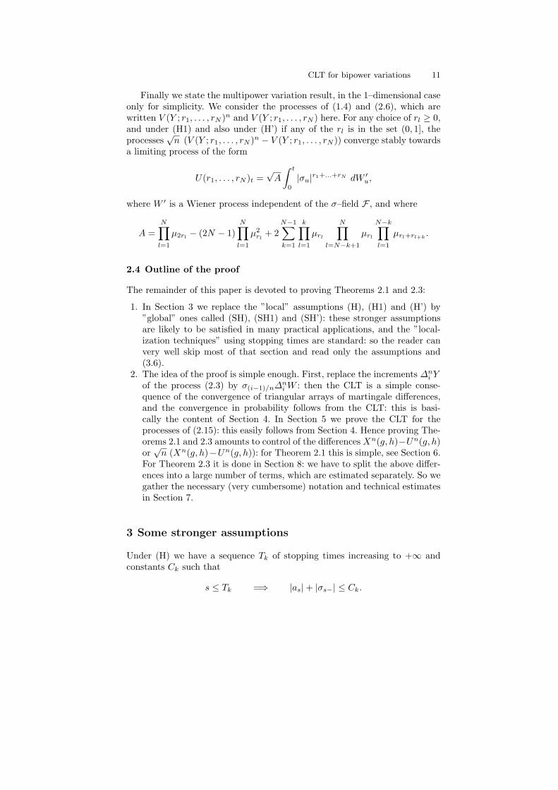
CLT for bipower variations 11
Finally we state the multipower variation result, in the 1–dimensional caseonly for simplicity. We consider the processes of (1.4) and (2.6), which arewritten V (Y ; r1, . . . , rN )n and V (Y ; r1, . . . , rN ) here. For any choice of rl ≥ 0,and under (H1) and also under (H’) if any of the rl is in the set (0, 1], theprocesses
√n (V (Y ; r1, . . . , rN )n − V (Y ; r1, . . . , rN )) converge stably towards
a limiting process of the form
U(r1, . . . , rN )t =√A
∫ t
0
|σu|r1+...+rN dW ′u,
where W ′ is a Wiener process independent of the σ–field F , and where
A =N∏l=1
µ2rl− (2N − 1)
N∏l=1
µ2rl
+ 2N−1∑k=1
k∏l=1
µrl
N∏l=N−k+1
µrl
N−k∏l=1
µrl+rl+k.
2.4 Outline of the proof
The remainder of this paper is devoted to proving Theorems 2.1 and 2.3:
1. In Section 3 we replace the ”local” assumptions (H), (H1) and (H’) by”global” ones called (SH), (SH1) and (SH’): these stronger assumptionsare likely to be satisfied in many practical applications, and the ”local-ization techniques” using stopping times are standard: so the reader canvery well skip most of that section and read only the assumptions and(3.6).
2. The idea of the proof is simple enough. First, replace the increments ∆ni Y
of the process (2.3) by σ(i−1)/n∆niW : then the CLT is a simple conse-
quence of the convergence of triangular arrays of martingale differences,and the convergence in probability follows from the CLT: this is basi-cally the content of Section 4. In Section 5 we prove the CLT for theprocesses of (2.15): this easily follows from Section 4. Hence proving The-orems 2.1 and 2.3 amounts to control of the differences Xn(g, h)−Un(g, h)or√n (Xn(g, h)−Un(g, h)): for Theorem 2.1 this is simple, see Section 6.
For Theorem 2.3 it is done in Section 8: we have to split the above differ-ences into a large number of terms, which are estimated separately. So wegather the necessary (very cumbersome) notation and technical estimatesin Section 7.
3 Some stronger assumptions
Under (H) we have a sequence Tk of stopping times increasing to +∞ andconstants Ck such that
s ≤ Tk =⇒ |as|+ |σs−| ≤ Ck.

12 O. E. Barndorff–Nielsen et al
Set a(k)s = as∧Tk
, and σ(k)s = σs if s < Tk and σ
(k)s = σTk− if s ≥ Tk. We
associate Y (k) with a(k) and σ(k) by (2.3), and Xn,(k)(g, h) with Y (k) by (2.1),and similarly X(k)(g, h) and U (k)(g, h) with σ(k) by (2.4) and (2.13) (and thesame process W ′ for all k).
Suppose that we have proved Theorem 2.1 for Xn,(k)(g, h), for each k.Observing that Xn,(k)(g, h)t = Xn(g, h)t and X(k)(g, h)t = X(g, h)t andU (k)(g, h)t = U(g, h)t for all t < Tk, and since Tk increases to ∞ as k →∞, itis obvious that the result of Theorem 2.1 also holds for Xn(g, h). So, insteadof (H), it is no restriction for proving Theorem 2.1 to assume the followingstronger hypothesis:
Hypothesis (SH): We have (H), and further the processes a and σ arebounded by a constant.
Now we proceed to strenghten (H1) in a similar manner. Assume (H1) andrecall the sequence (Sk) in (2.9): it is no restriction to assume in addition thatSk ≤ k. Set for k, l ≥ 1:
Ek,l = x ∈ E : ψk(x) > l, Rk,l = inf(t : µ((0, t]× Ek,l) ≥ 1).
Then we have
P(Rk,l ≤ Sk) ≤ E(µ((0, Sk]× Ek,l)) = F (Ek,l) E(Sk) ≤ k F (Ek,l).
In view of (2.9) we have liml→∞ F (Ek,l) = 0. Hence we find lk such thatP(Rk,lk < Sk) ≤ 2−k, and obviously the sequence of stopping times S′k =Sk ∧Rk,lk has supk S′k = ∞ a.s.
Next, just as above, we find a sequence S′′k of stopping times increasing to+∞ and constants Ck such that
s ≤ S′′k =⇒ ‖as‖+ ‖σs−‖+ ‖a′s‖+ ‖σ′s−‖+ ‖vs−‖ ≤ Ck.
Then if Tk = S′k ∧ S′′k , we still have supk Tk = ∞ a.s., and further
s ≤ Tk =⇒ ‖as‖+ ‖σs−‖+ ‖a′s‖+ ‖σ′s−‖+ ‖vs−‖ ≤ Ck,
µ((0, Tk)× Ek,lk) = 0.
. (3.1)
Set
a′(k)s =
a′s if s ≤ Tk
0 if s > Tk
(a(k)s , σ′(k)s , v(k)
s , w(k)(s, x)) =
(as, σ′s, vs, w(s, x)) if s < Tk
(0, 0, 0, 0) if s ≥ Tk,
µ(k)(ds, dx) = µ(ds, dx) 1Eck,lk
(x),
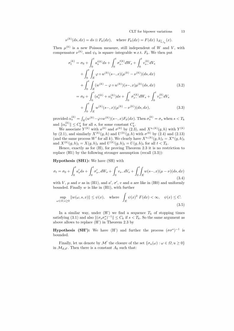
CLT for bipower variations 13
ν(k)(ds, dx) = ds⊗ Fk(dx), where Fk(dx) = F (dx) 1Eck,lk
(x).
Then µ(k) is a new Poisson measure, still independent of W and V , withcompensator ν(k), and ψk is square–integrable w.r.t. Fk. We then put
σ(k)t = σ0 +
∫ t
0
a′(k)s ds+∫ t
0
σ′(k)s− dWs +
∫ t
0
v(k)s−dVs
+∫ t
0
∫E
ϕ w(k)(s−, x)(µ(k) − ν(k))(ds, dx)
+∫ t
0
∫E
(w(k) − ϕ w(k))(s−, x)µ(k)(ds, dx) (3.2)
= σ0 +∫ t
0
(a′(k)s + α(k)s )ds+
∫ t
0
σ′(k)s− dWs +
∫ t
0
v(k)s−dVs
+∫ t
0
∫E
w(k)(s−, x)(µ(k) − ν(k))(ds, dx), (3.3)
provided α(k)s =
∫E
(w(k)−ϕw(k))(s−, x)Fk(dx). Then σ(k)s = σs when s < Tk
and ‖α(k)s ‖ ≤ C ′k for all s, for some constant C ′k.
We associate Y (k) with a(k) and σ(k) by (2.3), and Xn,(k)(g, h) with Y (k)
by (2.1), and similarly X(k)(g, h) and U (k)(g, h) with σ(k) by (2.4) and (2.13)(and the same process W ′ for all k). We clearly have Xn,(k)(g, h)t = Xn(g, h)tand X(k)(g, h)t = X(g, h)t and U (k)(g, h)t = U(g, h)t for all t < Tk.
Hence, exactly as for (H), for proving Theorem 2.3 it is no restriction toreplace (H1) by the following stronger assumption (recall (3.3)):
Hypothesis (SH1): We have (SH) with
σt = σ0 +∫ t
0
a′sds+∫ t
0
σ′s−dWs +∫ t
0
vs−dVs +∫ t
0
∫E
w(s−, x)(µ− ν)(ds, dx)
(3.4)with V , µ and ν as in (H1), and a′, σ′, v and a are like in (H0) and uniformlybounded. Finally w is like in (H1), with further
supω∈Ω,s≥0
‖w(ω, s, x)‖ ≤ ψ(x), where∫E
ψ(x)2 F (dx) <∞, ψ(x) ≤ C.
(3.5)
In a similar way, under (H’) we find a sequence Tk of stopping timessatisfying (3.1) and also ‖(σsσ?s )−1‖ ≤ Ck if s < Tk. So the same argument asabove allows to replace (H’) in Theorem 2.3 by
Hypothesis (SH’): We have (H’) and further the process (σσ?)−1 isbounded.
Finally, let us denote by M′ the closure of the set σu(ω) : ω ∈ Ω, u ≥ 0in Md,d′ . Then there is a constant A0 such that:
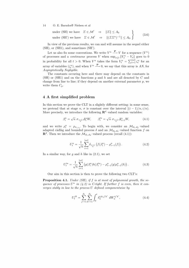
14 O. E. Barndorff–Nielsen et al
under (SH) we have Σ ∈M′ ⇒ ‖Σ‖ ≤ A0
under (SH’) we have Σ ∈M′ ⇒ ‖(ΣΣ?)−1‖ ≤ A0.
(3.6)
In view of the previous results, we can and will assume in the sequel either(SH), or (SH1), and sometimes (SH’).
Let us also fix some conventions. We write V n P−→ V for a sequence (V n)of processes and a continuous process V when sups≤t ‖V ns − Vs‖ goes to 0in probability for all t > 0. When V n takes the form V nt =
∑[nt]i=1 ζ
ni for an
array of variables (ζni ), and when V n P−→ 0, we say that this array is AN, forAsymptotically Negligible.
The constants occuring here and there may depend on the constants in(SH) or (SH1) and on the functions g and h and are all denoted by C andchange from line to line; if they depend on another external parameter p, wewrite them Cp.
4 A first simplified problem
In this section we prove the CLT in a slightly different setting: in some sense,we pretend that at stage n, σ is constant over the interval [(i − 1)/n, i/n).More precisely, we introduce the following Rd–valued random variables:
βni =√n σ i−1
n∆niW, β′ni =
√n σ i−1
n∆ni+1W, (4.1)
and we write ρni = ρσi/n. To begin with, we consider an Md1,d2–valued
adapted cadlag and bounded process δ and an Md2,d3–valued function f onRd. Then we introduce the Md1,d3–valued process (recall (4.1)):
Unt =1√n
[nt]∑i=1
δ i−1n
(f(βni )− ρni−1(f)
). (4.2)
In a similar way, for g and h like in (2.1), we set
U ′nt =1√n
[nt]∑i=1
(g(βni )h(β′ni )− ρni−1(g)ρ
ni−1(h)
). (4.3)
Our aim in this section is then to prove the following two CLT’s:
Proposition 4.1. Under (SH), if f is at most of polynomial growth, the se-quence of processes Un in (4.2) is C-tight. If further f is even, then it con-verges stably in law to the process U defined componentwise by
U jkt =d1∑j′=1
d3∑k′=1
∫ t
0
δ′jk,j′k′
u dW ′j′k′u , (4.4)
CLT for bipower variations 15
where
d1∑l=1
d3∑m=1
δ′jk,lmu δ′j′k′,lm
u =d2∑
l,l′=1
(ρσu
(f lkf l′k′)− ρσu
(f lk)ρσu(f l
′k′))δjlu δ
j′l′
u ,
(4.5)and W ′ is a d1d3–dimensional Wiener process defined on an extension of(Ω,F , (F t)t≥0,P) and which is independent of the σ–field F .
Proposition 4.2. Under (SH) and if g and h are continuous with at mostpolynomial growth, the sequence of processes U ′n is C-tight. If further g andh are even, then it converges stably in law to the process U(g, h) described in(2.13).
Before proceeding to the proofs, let us mention the following estimates,which are obvious under (SH):
E(‖βni ‖q) + E(‖β′ni ‖q) ≤ Cq. (4.6)
Next, saying that f is of at most polynomial growth means that for someconstants C > 0 and p (we can always choose p ≥ 2),
x ∈ Rd ⇒ |f(x)| ≤ C(1 + ‖x‖p). (4.7)
Observe also that Propositions 4.1 and 4.2 imply respectively
1n
[nt]∑i=1
δ i−1nf(βni ) P−→
∫ t
0
δu ρσu(f) du, (4.8)
1n
[nt]∑i=1
g(βni )h(β′ni ) P−→∫ t
0
ρσu(g)ρσu
(h) du. (4.9)
Proof of Proposition 4.1. We have Unt =∑[nt]i=1 ζ
ni , where ζni =
δ i−1n
(f(βni )− ρni−1(f))/√n. Recalling (4.6) and (4.7), we trivially have
E(ζni |F i−1n
) = 0, E(‖ζni ‖4|F i−1n
) ≤ C
n2, (4.10)
E(ζn,jki ζn,j′k′
i |F i−1n
) =1n∆jk,j′k′
i−1n
,
where ∆jk,j′k′
u is the right side of (4.5). Moreover since σ is cadlag we deducefrom (4.7) that s 7→ ρσs
(f) also is cadlag. Thus by the Riemann integrabilitywe get
[nt]∑i=1
E(ζn,jki ζn,j′k′
i |F i−1n
) →∫ t
0
∆jk,j′k′
u du. (4.11)
16 O. E. Barndorff–Nielsen et al
Then (4.10) and (4.11) are enough to imply the tightness of the sequence(Un).
Now, assume further that f is even. Since the variables ∆niW and −∆n
iWhave the same law, conditionally on F i−1
n, we get
E(ζn,jki ∆niW
l|F i−1n
) =d2∑m=1
δjmi−1n
E(∆niW
l f(√n σ i−1
n∆niW )mk|F i−1
n) = 0.
(4.12)Next, letN be any bounded martingale on (Ω,F , (F t)t≥0,P), which is orthog-onal to W . For j and k fixed, we consider the martingale Mt = E(g(βni )jk|F t),for t ≥ i−1
n . Since W is an (F t)–Brownian motion, and since βni is a functionof σ(i−1)/n and of ∆n
iW , we see that (Mt)t≥(i−1)/n is also, conditionally onF (i−1)/n, a martingale w.r.t. the filtration which is generated by the processWt −W i−1
n. By the martingale representation theorem the process M is thus
of the form Mt = M i−1n
+∫ t
i−1nηsdWs for an appropriate predictable process η.
It follows that M is orthogonal to the process N ′t = Nt −N i−1
n(for t ≥ i−1
n ),or in other words the product MN ′ is an (F t)t≥ i−1
n–martingale. Hence
E(∆ni N g(
√n σ i−1
n∆niW )jk|F i−1
n) = E(∆n
i N′Mi/n|F i−1
n)
= E(∆ni N
′∆niM |F i−1
n) = 0,
and thusE(ζni ∆
ni N |F i−1
n) = 0. (4.13)
If we put together (4.10), (4.11), (4.12) and (4.13), we deduce the resultfrom Theorem IX.7.28 of [9]. ut
Proof of Proposition 4.2. A simple computation shows that U ′nt =∑[nt]+1i=2 ζni + γn1 − γn[nt]+1, where
ζni =1√n
(g(βni−1)(h(β
′ni−1)− ρni−2(h)) + (g(βni )− ρni−1(g))ρ
ni−1(h)
),
γni =1√n
(g(βni )− ρni−1(g)) ρni−1(h).
We trivially have (4.10), while (4.12) and (4.13) (for any bounded martin-gale N orthogonal to W ) are proved exactly as in the previous proposition. Wewill write ρni−2,i−1(g, h) =
∫g(σ i−1
nx)h(σ i−2
nx)ρ(dx), where ρ is the N (0, Id′)
law. An easy computation shows that

CLT for bipower variations 17
E(ζn,jki ζn,j′k′
i |F i−1n
)
=1n
d2∑l,l′=1
(g(βni−1)
jlg(βni−1)j′l′ (ρni−2(h
lkhl′k′)− ρni−2(h
lk)ρni−2(hl′k′))
+g(βni−1)jl ρni−1(h
l′k′) (ρni−2,i−1(gj′l′ , hlk)− ρni−2(h
lk)ρni−1(gj′l′))
+g(βni−1)j′l′ ρni−1(h
lk) (ρni−2,i−1(gjl, hl
′k′)− ρni−2(hl′k′)ρni−1(g
jl))
+ρni−1(hl′k′)ρni−1(h
lk) (ρni−1(gjlgj
′l′)− ρni−1(gjl)ρni−1(g
j′l′))).
and thus by (4.8) and since the components of g and h satisfy (4.7) and arecontinuous and σ is cadlag (hence in particular ρni−2,i−1(g, h)− ρni−2(gh) goesto 0, uniformly in i ≤ [nt] + 1), we get
[nt]+1∑i=2
E(ζn,jki ζn,j′k′
i |F i−1n
) →∫ t
0
A(σu, g, h)jk,k′j′ du.
Then exactly as in the previous proof we deduce that the processes∑[nt]i=1 ζ
ni
are C–tight, and that they converge stably in law to the process U(g, h) of(2.13) when further g and h are even.
On the other hand γni is the transpose of the jump at time i/n of theprocess Un of (4.2) when δu = ρσu(h∗) and f = g∗, so Proposition 4.1 yieldssupi≤[nt] ‖γni ‖
P−→ 0 for any t: hence the results. ut
5 A second simplified problem
So far Y has played no role, but it will come in this section. Recalling (4.1),we set
ξni =√n ∆n
i Y − βni , ξ′ni =√n ∆n
i+1Y − β′ni . (5.1)
Observe that
ξni =√n
(∫ in
i−1n
audu+∫ i
n
i−1n
(σu− − σ i−1n
)dWu
),
and a similar equality for ξ′ni , with the integrals between i/n and (i + 1)/n.Then under (SH) we have for any q ∈ [2,∞), by Burkholder Inequality:
E(‖√n ∆n
i Y ‖q) + E(‖ξni ‖q) + E(‖ξ′ni ‖q) ≤ Cq. (5.2)
We can now consider the processes Un(g, h) of (2.15): in view of (5.2), theconditional expectations in (2.15) are finite as soon as g and h have polynomialgrowth.
18 O. E. Barndorff–Nielsen et al
Theorem 5.1. Under (SH) and if g and h are continuous with at most poly-nomial growth, the sequence of processes Un(g, h) of (2.15) is C–tight. If fur-ther g and h are even, it converges stably in law to the processes U(g, h) of(2.13).
We first prove three lemmas. The first one is very simple:
Lemma 5.2. Let (ζni ) be an array of random variables satisfying for all t:
[nt]∑i=1
E(‖ζni ‖2|F i−1n
) P−→ 0. (5.3)
If further each ζni is F i+1n
–measurable, the array (ζni −E(ζni |F i−1n
)) is AN.
Proof. Of course the result is well known when ζni is F i/n–measurable. Oth-erwise, we set ηni = E(ζni |F i/n). This new array satisfies also (5.3) and nowηni is F i/n–measurable: so the array (ηni −E(ηni |F i−1
n)) is AN.
Next, (5.3) and Lenglart’s inequality (see e.g. I-3.30 in [9]) yield∑[nt]i=1 E(‖ζni ‖2|F i/n)
P−→ 0, so the afore mentionned well known result alsoyields that the array (ζni − ηni ) is AN, and the result follows. ut
Lemma 5.3. Under (SH) we have for all t > 0:
1n
[nt]∑i=1
E(‖ξni ‖2 + ‖βni+1 − β′ni ‖2
)→ 0. (5.4)
Proof. First, the boundedness of a yields
E(‖ξni ‖2) ≤ C
(1n
+ nE
(∫ in
i−1n
‖σu− − σ i−1n‖2du
)).
We also trivially have
E(‖βni+1 − β′ni ‖2) ≤ CE(‖σ in− σ i−1
n‖2)
≤ CnE
(∫ in
i−1n
(‖σu− − σ i−1n‖2 + ‖σu− − σ i
n‖2)du
).
Hence the left side of (5.4) is smaller than
C
(t
n+∫ t
0
E(‖σu− − σ[nu]/n‖2 + ‖σu− − σ([nu]+1)/n‖2) du).
Since σ is cadlag, the expectation above goes to 0 for all u except the fixedtimes of discontinuity of the process σ, that is for almost all u, and it staysbounded by a constant because of (SH): hence the result by Lebesgue’s theo-rem. ut
CLT for bipower variations 19
For further reference, the third lemma is stated in a more general setting:
• f and k are functions on Rd satisfying (4.7);
• γni , γ′ni , γ′′ni are Rd–valued variables,
• Zni = 1 + ‖γni ‖+ ‖γ′ni ‖+ ‖γ′′ni ‖ satisfies E((Zni )p) ≤ Cp.
(5.5)
Lemma 5.4. Under (5.5) and if further k is continuous and
1n
[nt]∑i=1
E(‖γ′ni − γ′′ni ‖2) → 0, (5.6)
then we have for all t > 0:
1n
[nt]∑i=1
E(f(γni )2(k(γ′ni )− k(γ′′ni ))2
)→ 0. (5.7)
Proof. Set θni = (f(γni )(k(γ′ni )− k(γ′′ni )))2 and mA(ε) = sup(|k(x) − k(y)| :‖x− y‖ ≤ ε, ‖x‖ ≤ A). For all ε ∈ (0, 1] and A > 1 we have
θni ≤ C(A2pmA(ε)2 +A4p1‖γ′ni −γ′′ni ‖>ε
+(Zni )4p(1‖γni ‖>A + 1‖γ′ni ‖>A + 1‖γ′′ni ‖>A)
)≤ C
(A2pmA(ε)2 +
A4p‖γ′ni − γ′′ni ‖2
ε2+
(Zni )4p+1
A
).
Then in view of (5.5) we get
1n
[nt]∑i=1
E(θni ) ≤ C
A2pmA(ε)2 +1A
+A4p
nε2
[nt]∑i=1
E(‖γ′ni − γ′′ni ‖2)
.
This holds for all ε ∈ (0, 1] and A > 1. Since mA(ε) → 0 as ε → 0, for everyA, (5.7) readily follows from (5.6). ut
Proof of Theorem 5.1. In view of Proposition 4.2, it is clearly enough toprove that Un(g, h)− U ′n
P−→ 0. Set
ζni =1√n
(g(√n∆n
i Y )h(√n ∆n
i+1Y )− g(βni )h(β′ni ))
(5.8)
and observe that ζni is F i+1n
-measurable and that Un(g, h)t−U ′nt =∑[nt]i=1(ζ
ni −
E(ζni |F i−1n
)). Then by Lemma 5.2 it suffices to prove that
[nt]∑i=1
E(‖ζni ‖2) → 0. (5.9)
20 O. E. Barndorff–Nielsen et al
For proving (5.9) it is clearly enough to consider the case where both gand h are 1–dimensional. Recalling
√n ∆n
i Y = βni + ξni , we then have
‖ζni ‖2 ≤C
n
(h(√n ∆n
i+1Y )2 (g(βni + ξni )− g(βni ))2
+g(βni )2 (h(βni+1 + ξni+1)− h(βni+1))2 + g(βni )2(h(βni+1)− h(β′ni ))2
).
Then (5.9) immediately follows from (4.6) and (5.2) and from Lemmas 5.3and 5.4. ut
6 Proof of Theorem 2.1
As stated in Section 2, we can and will assume (SH). We use the notation ζniof (5.8), and set
ηni = E(g(√n ∆n
i Y )h(√n ∆n
i+1Y )|F i−1n
), η′ni = ρni−1(g)ρni−1(h)
and V nt =∑[nt]i=1η
ni and V ′nt =
∑[nt]i=1η
′ni . Theorem 5.1 implies 1
n (Xn(g, h) −V n) P−→ 0, and Riemann integrability yields 1
n V′n → X(g, h) pointwise in ω
and locally uniformly in time. So we need to prove that 1n (V n − V ′n) P−→ 0.
Since ηni − η′ni =√n E(ζni |F i−1
n), it clearly suffices to prove that
1√n
[nt]∑i=1
E(‖ζni ‖) → 0. (6.1)
By the Cauchy–Schwarz inequality, the left side of (6.1) is smaller than(t∑[nt]i=1 E(‖ζni ‖2)
)1/2
, and thus (6.1) follows from (5.9). ut
7 Technical preliminaries for Theorem 2.3
As said before, for proving Theorem 2.3 we can and will assume (SH), and also(SH’) when at least one of the components of g or h satisfies (K’) instead of(K). In fact, this theorem is deduced from Theorem 5.1, provided we can showthat
√n (Xn(g, h)t − Un(g, h)t) goes to 0 in probability, locally uniformly in
t. This amounts to proving that the array
ζni =1√n
E(g(√n ∆n
i Y )h(√n ∆n
i+1Y )|F i−1n
)−√n
∫ in
i−1n
ρσu(g)ρσu
(h)du
is AN. Obviously, we can work componentwise, and so we will assume w.l.o.g.that both g and h are 1–dimensional (they still are functions on Rd, though).
CLT for bipower variations 21
We have ζni = ζ ′ni + ζ ′′ni , where
ζ ′ni =1√n
(E(g(
√n ∆n
i Y )h(√n ∆n
i+1Y )|F i−1n
)
−E(g(βni )|F i−1n
) E(h(β′ni )|F i−1n
)), (7.1)
ζ ′′ni =√n
∫ in
i−1n
(ρσu(g)ρσu(h)− ρni−1(g)ρni−1(h)) du. (7.2)
So we are left to prove that both arrays (ζ ′ni ) and (ζ ′′ni ) are AN. For the secondone this is relatively simple, but for the first one it is quite complicated, andwe need to split the difference in (7.1) into a large number of terms, which aretreated in different ways: this section is devoted to estimates for these variousterms.
7.1 Some notation
First, we fix a sequence of numbers εn ∈ (0, 1] (which will be chosen laterand satisfy ε2nn ≥ 1), and we set En = x ∈ E : ψ(x) > εn. Then, recallingthe product–matrix notation, under (SH1) we can introduce a (long) series ofRd–valued random variables:
ζ(1)ni =√n
∫ in
i−1n
(au − a i−1n
)du+√n
∫ in
i−1n
(∫ u
i−1n
a′sds
+∫ u
i−1n
(σ′s− − σ′i−1n
)dWs +∫ u
i−1n
(vs− − v i−1n
)dVs
)dWu,
ζ(1)′ni =√n
(∫ in
i−1n
a′sds+∫ i
n
i−1n
(σ′s− − σ′i−1
n
)dWs
+∫ i
n
i−1n
(vs− − v i−1n
)dVs
)∆ni+1W,
ζ(2)ni =√n
(1na i−1
n+ σ′i−1
n
∫ in
i−1n
(Wu −W i−1n
)dWu
+v i−1n
∫ in
i−1n
(Vu− − V i−1n
)dWu
),
ζ(2)′ni =√n(σ′i−1
n
∆niW + v i−1
n∆ni V)∆ni+1W,
ζ(3)ni =√n
∫ in
i−1n
(∫ u
i−1n
∫Ec
n
w(s−, x)(µ− ν)(ds, dx)
)dWu,
ζ(3)′ni =√n
(∫ in
i−1n
∫Ec
n
w(s−, x)(µ− ν)(ds, dx)
)∆ni+1W,
22 O. E. Barndorff–Nielsen et al
ζ(4)ni = −√n
∫ in
i−1n
(∫ u
i−1n
∫En
(w(s−, x)− w(i− 1n
, x)) ν(ds, dx)
)dWu,
ζ(4)′ni = −√n
(∫ in
i−1n
∫En
(w(s−, x)− w(i− 1n
, x)) ν(ds, dx)
)∆ni+1W,
ζ(5)ni = −√n
∫ in
i−1n
(∫ u
i−1n
∫En
w(i− 1n
, x) ν(ds, dx)
)dWu,
ζ(5)′ni = −√n
(∫ in
i−1n
∫En
w(i− 1n
, x) ν(ds, dx)
)∆ni+1W,
ζ(6)ni =√n
∫ in
i−1n
(∫ u
i−1n
∫En
(w(s−, x)− w(i− 1n
, x)) µ(ds, dx)
)dWu,
ζ(6)′ni =√n
(∫ in
i−1n
∫En
(w(s−, x)− w(i− 1n
, x)) µ(ds, dx)
)∆ni+1W,
ζ(7)ni =√n
∫ in
i−1n
(∫ u
i−1n
∫En
w(i− 1n
, x) µ(ds, dx)
)dWu,
ζ(7)′ni =√n
(∫ in
i−1n
∫En
w(i− 1n
, x) µ(ds, dx)
)∆ni+1W.
We also set
ξni = ζ(1)ni + ζ(3)ni + ζ(4)ni + ζ(6)ni , ξni = ζ(2)ni + ζ(5)ni + ζ(7)ni
ξ′′ni = ζ(1)′ni + ζ(3)′ni + ζ(4)′ni + ζ(6)′ni ,
ξ′′ni = ζ(2)′ni + ζ(5)′ni + ζ(7)′ni
ξ′ni = ξni+1 + ξ′′ni , ξ′ni = ξni+1 + ξ′′ni .
(7.3)
In view of (5.1), a tedious but simple computation shows that
√n ∆n
i Y − βni = ξni = ξni + ξni ,√n ∆n
i+1Y − β′ni = ξ′ni = ξ′ni + ξ′ni . (7.4)
Next, we put ϕ(ε) =∫‖ψ(x)‖≤ε ψ(x)2F (dx), so that
ε ↓ 0 ⇒ ϕ(ε) → 0
θ ∈ [0, 2] ⇒∫ψ(x)>ε ψ(x)θF (dx) ≤ C
ε2−θ ,
θ ≥ 2 ⇒∫ψ(x)≤ε ψ(x)θF (dx) ≤ ϕ(ε) εθ−2.
(7.5)
Finally, set

CLT for bipower variations 23
αn,qi =1
nq/2+ E
((n
∫ in
i−1n
(‖au − a i−1
n‖2 + ‖σ′u− − σ′i−1
n
‖2 + ‖vu− − v i−1n‖2
+∫E
‖w(u−, x)− w(i− 1n
, x)‖2F (dx))du
)q/2), (7.6)
7.2 Estimates for ζ(k)nj and ζ(k)′n
j
Here we estimate moments of the variables ζ(k)ni and ζ(k)′ni . A repeated useof the Holder and Burkholder inequalities gives us for q ≥ 2, and under (SH1):
E(‖ζ(1)ni ‖q) + E(‖ζ(1)′ni ‖q) ≤ Cq αn,qi /nq/2,
E(‖ζ(2)ni ‖q) + E(‖ζ(2)′ni ‖q) ≤ Cq/nq/2.
(7.7)
Lemma 7.1. Under (SH1), and for any even integer q ≥ 2, we have
E(‖ζ(3)ni ‖q) + E(‖ζ(3)′ni ‖q) ≤ Cq ϕ(εn)εq−2n
n. (7.8)
Proof. Apply the Holder and Burkholder inequalities repeatedly to get
E(‖ζ(3)ni ‖q) ≤ CqE
n ∫ i
n
i−1n
∥∥∥∥∥∫ u
i−1n
∫Ec
n
w(s, x)(µ− ν)(ds, dx)
∥∥∥∥∥2
du
q/2
≤ Cq n
∫ in
i−1n
E
(∥∥∥∥∥∫ u
i−1n
∫Ec
n
w(s, x)(µ− ν)(ds, dx)
∥∥∥∥∥q
du
)
≤ Cq n
∫ in
i−1n
E
(∫ u
i−1n
∫Ec
n
‖w(s, x)‖2µ(ds, dx)
)q/2 du
≤ Cq E
(∫ in
i−1n
∫Ec
n
ψ(x)2µ(ds, dx)
)q/2 :
= E((Znin− Zni−1
n
)q/2),
where Znt =∫ t0
∫Ec
nψ(x)2µ(ds, dx) is an increasing pure jump Levy process,
whose Laplace transform is
λ 7→ E(e−λ(Zns+t−Z
ns )) = exp t
∫Ec
n
(e−λψ(x)2 − 1
)F (dx).
We compute the q/2–moment of Zns+t−Zns by differentiating q/2 times theLaplace transform at 0: this is the sum, over all choices u1, . . . , uk of positiveintegers with
∑ki=1 ui = q/2, of suitable constants times the product for all
24 O. E. Barndorff–Nielsen et al
i = 1, . . . , k of the terms t∫Ec
nψ(x)2uiF (dx); moreover this term is smaller
than tε2ui−2n ϕ(εn). Since further εn ≤ 1 and ϕ(1) <∞, we deduce that
E((Zns+t − Zns )q/2) ≤ Cqϕ(εn)q/2∑k=1
tkεq−2kn ≤ Cqϕ(εn)(tεq−2
n + tq/2).
We deduce (7.8) for ζ(3)ni (recall nε2n ≥ 1), and the same holds for ζ(3)′ni . ut
Lemma 7.2. Under (SH1), for any q > 2 we have
E(‖ζ(4)ni ‖q) + E(‖ζ(4)′ni ‖q) + E(‖ζ(5)ni ‖q) + E(‖ζ(5)′ni ‖q) ≤Cqεqn nq
. (7.9)
Proof. Applying the Holder and Burkholder inequalities and ‖w(s, x)‖ ≤ψ(x) yields for j = 4, 5:
E(‖ζ(j)ni ‖q + ‖ζ(j)′ni ‖q) ≤
≤ CqE
n ∫ i
n
i−1n
(∫ u
i−1n
∫En
ψ(x)ν(ds, dx)
)2
du
q/2
≤ Cq
(∫ in
i−1n
ds
∫En
ψ(x)F (dx)
)q≤ Cqnq
(∫En
ψ(x)F (dx))q. (7.10)
The result readily follows from (7.5). ut
For ζ(j)ni and ζ(j)′ni with j = 6, 7 the analogous estimates are noy quiteenough for our purposes, and we need a bit more. Below, we consider a pair(r,B), where r ∈ (0, 1] and B is a closed subset of Rd, with Lebesgue measure0, and such that (2.11) holds when r < 1 and that r = 1 if B = ∅. Let also
r = 1 ⇒ γni = 1
r < 1 ⇒ γni = 1 + 1d(γn
i ,B) , with either γni = βni or γni = β′ni
(7.11)
Lemma 7.3. Under (SH1) and the previous assumptions, and if further(SH’) holds whenever r < 1, for any q ∈ (1, 2) and l ∈ [0, 1) we can findu > 1 (depending on q and l) such that
E(‖ζ(6)ni ‖q (γni )l
)+ E
(‖ζ(6)′ni ‖q (γni )l
)≤ Cl,q (αn,2
i )1/u
nq/2 ,
E(‖ζ(7)ni ‖q (γni )l
)+ E
(‖ζ(7)′ni ‖q (γni )l
)≤ Cl,q
nq/2 .
(7.12)
CLT for bipower variations 25
Proof. We set Mni = sups∈[(i−1)/n,i/n] ‖Ws − W i−1
n‖ and wn(s, x) =
w(s−, x)− w( i−1n , x) for i−1
n < s ≤ in , and
Znt =∫ t
0
∫En
ψ(x) µ(ds, dx), Z ′nt =∫ t
0
∫En
‖wn(s, x)‖ µ(ds, dx).
Observe that Zn and Z ′n are nondecreasing, piecewise constant, and Z ′nt −Z ′ns ≤ 2(Znt − Zns ) whenever s < t. Then
‖ζ(6)ni ‖ ≤ C√n Mn
i (Z ′nin− Z ′ni−1
n
).
Set u′ = 12
(1 + 1
l
∧1q−1
), which satisfies u′ > 1 because l < 1 and q ∈ (1, 2).
With δni = (√nMn
i )u′q (γni )u
′l we then have (since u′ > 1 and u′q−u′+1 > 0):
‖ζ(6)ni ‖q (γni )l ≤ Cq
(δni (Zni
n− Zni−1
n
)u′q−u′+1
) 1u′ (Z ′ni
n− Z ′ni−1
n
)u′−1
u′ ,
and Holder’s inequality yields
E(‖ζ(6)ni ‖q(γni )l
)≤ Cq
(E(δni (Zni
n− Zni−1
n
)u′q−u′+1
)) 1u′(E(Z ′ni
n− Z ′ni−1
n
))u′−1
u′. (7.13)
Now, if we combine (2.11) and (3.6), we see that when r < 1 (so (SH’)holds) the variable d(γni , B) has a conditional law knowing F i−1
nwhich has
a density which is bounded uniformly in n, i and ω, so E((γni )s|F i−1n
) isbounded by a constant Cs for all s ∈ [0, 1), whether r = 1 or r < 1. Also,E((
√n Mn
i )p|F i−1n
) ≤ Cq for all p > 0. Then by Holder’s inequality we get
E(δni |F i−1
n
)≤ Cq,l. Since further the variable Zni
n
− Zni−1n
is independent ofδni , conditionally on F i−1
n, we deduce
E(δni (Zni
n− Zni−1
n
)u′q−u′+1
)≤ Cq,l E((Zni
n− Zni−1
n
)u′q−u′+1). (7.14)
Next, we estimate the moments of Zn and Z ′n. Observe that Z ′n = A′n +N ′n, where
A′nt =∫ t
0
∫En
‖wn(s, x)‖ν(ds, dx), N ′n =∫ t
0
∫En
‖wn(s, x)‖(µ− ν)(ds, dx).
On the one hand, since F (En) ≤ C/ε2n by (7.5) and nε2n ≥ 1,
(A′nin−A′ni−1
n
)2 ≤ 1n
∫ in
i−1n
ds
(∫En
‖wn(s, x)‖ F (dx))2
≤ 1n
∫ in
i−1n
ds F (En)∫En
‖wn(s, x)‖2 F (dx)
≤∫ i
n
i−1n
ds
∫En
‖wn(s, x)‖2 F (dx).
26 O. E. Barndorff–Nielsen et al
On the other hand N ′n is a square–integrable martingale, and thus
E((N ′n
in−N ′n
i−1n
)2)≤ E
(∫ in
i−1n
ds
∫En
‖wn(s, x)‖2F (dx)
),
and thus
E((Z ′ni
n− Z ′ni−1
n
)2)≤ C αn,2i
n. (7.15)
If we replace ‖wn(s, x)‖ by ψ(x), we obtain in a similar fashion
E((Zni
n− Zni−1
n
)2)≤ C
n. (7.16)
Then if we combine (7.13), (7.14), (7.15) and (7.16), and since u′q−u′+1 ≤ 2,we obtain the result for ζ(6)ni , with u = 2u′
u′−1 > 1, and the proof for ζ(6)′ni issimilar. Finally if we replace wn by w (then αn,2i is replaced by a constant),we get the result for ζ(7)ni and ζ(7)′ni . ut
7.3 Estimates for the variables of (7.3)
Here we derive estimates on the variables defined in (7.3). Below, the pair(B, r) and the variable γni are like in Lemma 7.3. We also consider positiverandom variables Zni which satisfy
E((Zni )q) ≤ Cq ∀q ≥ 2. (7.17)
Observe that ξni and ξ′ni do not depend on the sequence εn, but ξni and ξ′nido. Remember also the variables αn,qi defined ibn (7.6).
Lemma 7.4. Assume (SH1) and (SH’) and (7.11) with r < 1 and (7.17).Let p ≥ 2 and l ∈ (0, 1). Then if θ ∈ (1, 2) we have
E((Zni )p ‖ξni ‖θ (γni )l) + E((Zni )p ‖ξ′ni ‖θ (γni )l) ≤ Cp,θ,lnθ/2
, (7.18)
Moreover one can find a sequence εn > 0 with nε2n ≥ 1 and a sequence zn > 0with zn → 0, both sequences depending on l only, and also two numbers q, q′ ≥1 depending on l only, such that
E((Zni )p‖ξni ‖(γni )l) ≤ Cp,l√n
(zn + (αn,qi )1/q + (αn,2i )1/q′),
E((Zni )p‖ξ′ni ‖(γni )l)) ≤ Cp,l√n
(zn + (αn,qi )1/q + (αn,qi+1)1/q
+(αn,2i )1/q′+ (αn,2i+1)
1/q′).
(7.19)
CLT for bipower variations 27
Proof. We prove (7.18) and (7.19) for ξni and ξni only, the proofs for ξ′ni andξ′ni being similar. We have seen in the proof of Lemma 7.3 that, by (7.11),
s ∈ [0, 1) ⇒ E((γni )s) ≤ Cs. (7.20)
Although ξni does not depend on the sequence εn, we need to introduce asuitable sequence εn to prove (7.18): so we prove (7.18) and (7.19) simulta-neously, with some fixed θ ∈ [1, 2) for the first result, and with θ = 1 for thesecond one. If t = 1
2
(1 + 1
l
∧2θ
), by (7.17) and Holder’s inequality we get
E((Zni )p ‖ξni ‖θ (γni )l) ≤ Cp,θ,l(E(‖ξni ‖tθ (γni )tl)
)1/t,
E((Zni )p ‖ξni ‖ (γni )l) ≤ Cp,l
(E(‖ξni ‖t (γni )tl)
)1/t
.
(7.21)
Next, let s be the biggest number in (1, 1/tl) such that its conjugateexponent s′ is of the form s′ = 2m/tθ for some m ∈ N with m ≥ 2,and put q = s′tθ. Note that s′ and q depend on θ and l only. The sety > 0 : yqϕ(y/
√n) ≤ 1 is an open or semi–open interval whose left end
point is 0, and whose right end point is denoted by a′n, and since ϕ(y) → 0as y → 0 it is clear that a′n → ∞. At this point, we set an = 1
∨(a′n − 1/n):
then an → ∞, and for all n big enough an < a′n and thus aqnϕ(an/√n) ≤ 1.
Then we choose the sequence εn as εn = an/√n, thus nε2n ≥ 1. Observe that
both sequences εn and an only depend on θ and l.Now we apply (7.8) and (7.9) with q and εn as above, plus (7.20) and
Holder’s inequality, to get(E(‖ζ(3)ni ‖tθ (γni )tl
)1/t ≤ Cθ,l ϕ(εn)1/s′t aθ−2/s′tn
nθ/2 ≤ Cθ,l
nθ/2a2/s′tn
≤ Cθ,l
nθ/2 ,(E(‖ζ(4)ni ‖tθ (γni )tl
)1/t +(E(‖ζ(5)ni ‖tθ (γni )tl
)1/t ≤ Cθ,l
nθ/2aθn≤ Cθ,l
nθ/2 .
(7.22)
In a similar way, (7.20) and (7.7) and Holder’s inequality give (with the sameq as above): (
E(‖ζ(1)ni ‖tθ (γni )tl)1/t ≤ Cθ,l (αn,q
i )θ/q
nθ/2 ,(E(‖ζ(2)ni ‖tθ (γni )tl
)1/t ≤ Cθ,l
nθ/2 .
(7.23)
Finally applying (7.12) and tθ < 2 yields(E(‖ζ(6)ni ‖tθ (γni )tl
)1/t ≤ Cθ,l (αn,2i )1/q′
nθ/2 ,(E(‖ζ(7)ni ‖tθ (γni )tl
)1/t ≤ Cθ,l
nθ/2
(7.24)
for some q′ > 1 depending on tθ and tl, hence on θ and l only.Then if we put together (7.21), (7.22), (7.23) and (7.24), and in view of
(7.3) and (7.4), we readily get (7.18), and also (7.19) with zn = a−2/s′tn + a−1
n
(note that for (7.19) we take θ = 1). ut

28 O. E. Barndorff–Nielsen et al
7.4 Final estimates
The previous subsection gave us estimates on the variables of (7.3), which inview of (7.4) are the building blocks for obtaining the difference occuring in(7.1). Now we procees to give estimates for this difference itself. We start witha lemma about the variables of (7.6).
Lemma 7.5. Under (SH1) we have for all q ≥ 2 and q′ ≥ 1 and t > 0:
αn,qi ≤ Cq,1n
[nt]∑i=1
(αn,qi )1/q′→ 0. (7.25)
Proof. We can of course forget about the term 1/nq/2 in (7.6), whereas thefirst part of (7.25) is obvious. For the second part we set
γn(u) = ‖au − a[nu]/n‖2 + ‖σ′u− − σ′[nu]/n‖2 + ‖vu− − v[nu]/n‖2
+∫E
‖w(u−, x)− w(i− 1n
, x)‖2F (dx).
Then the Holder inequality yields
1n
[nt]∑i=1
(αn,qi )1/q′≤ [nt]
n
1[nt]
[nt]∑i=1
E
(n ∫ in
i−1n
γn(u)du
)q/21/q′
≤ [nt]n
1[nt]
[nt]∑i=1
E
(n
∫ in
i−1n
γn(u)q/2du
)1/q′
≤ tq′−1
q′
(E(∫ t
0
γn(u)q/2du))1/q′
.
Since γn is uniformly bounded and converges pointwise to 0, we get the result.ut
Let us now introduce a list of growth or smoothness assumptions on a real–valued function f on Rd, with complement (4.7). Below, C > 0 and p ≥ 2are suitable constants, and the pair (B, r) is given, with the properties statedbefore (7.11). We list some conditions, for which we assume that f is differ-entiable on the complement Bc. Below, each ΨA is an increasing continuousfunction on R+ with ΨA(0) = 0.
x ∈ Bc ⇒ |∇f(x)| ≤ C(1 + ‖x‖p)(
1 +1
d(x,B)1−r
), (7.26)
x, y ∈ Rd ⇒ |f(x+ y)− f(x)| ≤ C(1 + ‖x‖p + ‖y‖p) ‖y‖r, (7.27)
CLT for bipower variations 29
‖x‖ ≤ A, 0 < ‖y‖ ≤ ε < d(x,B) ⇒ ‖∇f(x+ y)−∇f(x)‖ ≤ ΨA(ε) (7.28)
0 < ‖y‖ ≤ d(x,B)2
=⇒ ‖∇f(x+ y)−∇f(x)‖ ≤ C(1 + ‖x‖p + ‖y‖p) ‖y‖d(x,B)2−r
.(7.29)
The connections with our assumptions (K) and (K’) are as follows (with Band r identical in (K’) and above, or B = ∅ and r = 1 in the case of (K)):
(K), or (K’) with r = 1 ⇒ (4.7), (7.26), (7.27) and (7.28), (7.30)
(K’) with r < 1 ⇒ (4.7) , (7.26), (7.27) and (7.29) (7.31)
Next, we consider the setting of (5.5), with k is differentiable on Bc. Welet γ′′ni be either βni or β′ni , and we introduce the following subsets of Ω:
Ani = ‖γ′ni − γ′′ni ‖ > d(γ′′ni , B)/2, (7.32)
(observe that Ani = ∅ when B = ∅). Let also γni be an auxiliary variable whichfor each ω is on the segment joining γ′ni and γ′′ni , and let γni be 1 when r = 1and 1 + 1/d(γ′′ni , B) when r < 1. Then we set
Φni = f(γni )((k(γ′ni )− k(γ′′ni ))1An
i−∇k(γ′′ni )(γ′ni − γ′′ni )1An
i
+(∇k(γni )−∇k(γ′′ni ))(γ′ni − γ′′ni )1(Ani )c
)(7.33)
Φni = f(γni ) ∇k(γ′′ni )(γ′ni − γ′′ni ) (7.34)
(by the fact that B has Lebesgue measure 0, we see that k is a.s. differentiableat the point γ′′ni , which is either βni or β′ni , so (7.33) and (7.34) make sense).
Lemma 7.6. Assume the following:(i) (SH1) and (5.5) and k satisfies (7.26) and (7.27);(ii) if r = 1 then k satisfies (7.28);(iii) if B 6= ∅ then (SH’) holds;(iv) if r < 1 then k satisfies (7.29).
(a) If γ′′ni = βni and γ′ni − γ′′ni = ξni , or if γ′′ni = β′ni and γ′ni − γ′′ni = ξ′ni , wehave for all t > 0:
1√n
[nt]∑i=1
E(|Φni |) → 0. (7.35)
(b) If γ′′ni = βni and γ′ni − γ′′ni = ξni , or if γ′′ni = β′ni and γ′ni − γ′′ni = ξ′ni , wehave for all t > 0:
1√n
[nt]∑i=1
E(|Φni |) → 0. (7.36)
30 O. E. Barndorff–Nielsen et al
Proof. 1) We first prove the two results when r = 1. We choose εn = 1 forall n and putting together all estimates in (7.7), (7.8), (7.9) and (7.12) (withl = 0, so this estimate holds for q = 2 as well) to get
q ≥ 2 ⇒ E(‖γ′ni − γ′′ni ‖q) ≤ Cqn. (7.37)
Then (4.7) and (7.26) and the property Ani ⊂ d(γ′′ni , B) < ε∪‖γ′ni −γ′′ni ‖ ≥ε/2 yield for all A > 0, ε > 0:
|Φni |+ |Φni | ≤ C(Zni )2p(ΨA(ε) +
‖γ′′ni ‖A
+‖γ′ni − γ′′ni ‖
ε+ 1d(γ′′ni ,B)≤ε
)‖γ′ni − γ′′ni ‖. (7.38)
If B = ∅ the indicator function above vanishes. Otherwise, the variable γ′′nihas a conditional law knowing F i−1
nwhich has a density (on Rd) that is
smaller than some (non–random) Lebesgue integrable function φ (see (3.6)),so it also has an unconditional density smaller than φ. Therefore
P(d(γ′′ni , B) ≤ ε) ≤ αε :=∫x:d(x,B)≤ε
φ(x)dx,
and limε→0 αε = 0. Then (5.5), (7.37), (7.38) and the multivariate Holderinequality yield
E(|Φni |) + E(|Φni |) ≤C√n
(ΨA(ε) +
1A
+1
εn1/4+ α1/4
ε
).
Hence (7.35) readily follows: choose A big, then ε small.
2) Now we suppose that r < 1, hence B 6= ∅. We have
|Φni | ≤ (Zni )2p(‖γ′ni − γ′′ni ‖r 1An
i+ ‖γ′ni − γ′′ni ‖ 1An
i
+‖γ′ni − γ′′ni ‖d(γ′′ni , B)1−r
1Ani
+‖γ′ni − γ′′ni ‖2
d(γ′′ni , B)2−r1(An
i )c
)≤ C(Zni )2p ‖γ′ni − γ′′ni ‖1+r/2 (γni )1−r/2, (7.39)
where the first inequality follows from (7.26), (7.27) and (7.29) for k, whilethe second one is obtained by using the definition of the set Ani . We also have
|Φni | ≤ C(Zni )2p ‖γ′ni − γ′′ni ‖ (γni )1−r. (7.40)
Therefore, Lemma 7.4 readily gives (7.35), and also (7.36) if we further useLemma 7.5. ut
CLT for bipower variations 31
8 Proof of Theorem 2.3
1) As said at the beginning of the previous Section, we can assume that gand h are 1–dimensional, and that (SH1), and also (SH’) when either g or hsatisfies (K’) instead of (K), and we need to prove that the arrays defined in(7.1) and (7.1) are AN.
2) Let us prove first that (ζ ′′ni ) is AN. If f is continuously differentiable, and fand ∇f have polynomial growth, we readily deduce from Lebesgue’s theoremthat Σ 7→ ρΣ(f) = E(f(ΣU)) (where U is an N (0, Id)–random vector) isbounded, continuously differentiable and with bounded derivatives over theset M′ defined in connection with formula (3.6). Hence if both g and h satisfy(K) we have (recall the notation (3.6), and set φ(Σ) = ρΣ(g)ρΣ(h)):
Σ, Σ′ ∈M′ ⇒
|φ(Σ)|+ ‖∇φ(Σ)‖ ≤ C
|φ(Σ)− φ(Σ′)| ≤ C‖Σ −Σ′‖
|φ(Σ)− φ(Σ′)−∇φ(Σ′)(Σ −Σ′)‖≤ Ψ(‖Σ −Σ′|)‖Σ −Σ′‖
(8.1)
for some constant C (depending on A0 in (3.6)) and some increasing functionΨ on R+, continuous and null at 0 (here,∇φ isMd,d–valued, and∇φ(Σ′)(Σ−Σ′) is R–valued).
If g or h (or both) satisfy (K’) only we also have (SH’), and since
ρΣ(f) =∫
1(2π)d/2det(ΣΣ?)1/2
f(x) exp(−1
2x?(ΣΣ?)−1x
)dx
we see that as soon as f has polynomial growth the function Σ 7→ ρΣ(f) isC∞ with bounded derivatives of all orders on the set M′. Hence we also have(8.1), which thus holds in all cases.
Since we can write (7.2) as ζ ′′ni =√n∫ i/n(i−1)/n
(φ(σu) − φ(σ(i−1)/n)du, wehave ζ ′′ni = ηni + η′ni where
ηni =√n ∇φ(σ i−1
n)∫ i
n
i−1n
(σu − σ i−1n
) du,
η′ni =√n
∫ in
i−n
(φ(σu)− φ(σ i−1
n)−∇φ(σ i−1
n)(σu − σ i−1
n))du.
and we need to prove that the two arrays (ηni ) and (η′ni ) are AN.We decompose further ηni as ηni = µni + µ′ni , where
µni =√n ∇φ(σ i−1
n)∫ i
n
i−1n
du
∫ u
i−1n
a′sds,
32 O. E. Barndorff–Nielsen et al
µ′ni =√n ∇φ(σ i−1
n)∫ i
n
i−1n
(∫ u
i−1n
σs−dWs +∫ u
i−1n
vs−dVs
+∫ u
i−1n
∫E
w(s−, x)(µ− ν)(ds, dx)
)du.
On the one hand, we have |µni | ≤ C/n3/2 by (8.1) and the boundedness of a′,so the array (µni ) is AN. On the other hand, we also get by (SH1) and (8.1)and Cauchy–Schwarz applied twice:
E(µ′ni |F i−1n
) = 0, E((µ′ni )2|F i−1n
) ≤ C
n3.
Then the array (µ′ni ) is AN, as well as the array (ηni ).Finally, using (8.1) once more, we see that for all ε > 0,
|η′ni | ≤√n
∫ in
i−1n
Ψ(‖σu − σ i−1n‖) ‖σu − σ i−1
n‖ du
≤√n Ψ(ε)
∫ in
i−1n
‖σu − σ i−1n‖ du+
C√n
ε
∫ in
i−1n
‖σu − σ i−1n‖2 du.
Since E(‖σu − σ i−1n‖2) ≤ C/n when u ∈ ((i− 1)/n, i/n], we deduce that
[nt]∑i=1
E(|η′ni |) ≤ Ct
(Ψ(ε) +
1ε√n
).
From this we deduce the AN property of the array (η′ni ) because ε > 0 isarbitrarily small and limε→0 Ψ(ε) = 0. Hence, finally, the array (ζ ′′ni ) is AN.
3) Now we start proving that the array (ζ ′ni ) also is AN. Since φ(σ(i−1)/n) =E(g(βni )h(β′ni )|F i−1
n), we have ζ ′ni = E(δni |F i−1
n), where
δni =1√n
(g(√n ∆n
i Y )h(√n ∆n
i+1Y )− g(βni )h(β′ni )).
Let us setAni = ‖
√n ∆n
i Y − βni ‖ > d(βni , B)/2,
A′ni = ‖√n ∆n
i+1Y − β′ni ‖ > d(β′ni , B′)/2,
where B (resp. B′) is either empty or is the set associated with g (resp. h),according to whether that function satisfies (K) or (K’). We can express thedifference g(
√n ∆n
i Y ) − g(βni ) using a Taylor expansion if we are on the set(Ani )
c, and we can thus write
CLT for bipower variations 33
g(√n ∆n
i Y )− g(βni )= (g(
√n ∆n
i Y )− g(βni ))1Ani−∇g(βni )(
√n ∆n
i Y − βni )1Ani
+(∇g(γni )−∇g(βni ))(√n ∆n
i Y − βni ) 1(Ani )c
+∇g(βni )(√n ∆n
i Y − βni ), (8.2)
where γni is some (random) vector lying on the segment between√n ∆n
i Yand βni : recall that ∇g(γni ) is well defined because on (Ani )
c we have γni ∈ Bc,while ∇g(βni ) is a.s. well defined because either B is empty, or it has Lebesguemeasure 0 and βni has a density. Analogously, h(
√n ∆n
i+1Y )− h(β′ni ) can bewritten likewise, provided we replace ∆n
i Y , βni , Ani , γni by ∆n
i+1Y , β′ni , A′ni ,γ′ni .
Now observe that
δni =1√ng(√n ∆n
i Y )(h(√n ∆n
i+1Y )− h(β′ni ))
+1√n
(g(√n ∆n
i Y )− g(βni ))h(β′ni ),
Therefore we deduce from the decomposition (8.2) and the analogous one forh, and also from (7.3) and (7.4), that δni =
∑6k=1 δ
ni (k), where
δni (1) =1√ng(√n ∆n
i Y )∇h(β′ni )ξ′′ni ,
δni (2) =1√ng(√n ∆n
i Y )∇h(β′ni )ξni+1,
δni (3) =1√nh(β′ni )∇g(βni )ξni ,
δni (4) =1√n
(g(√n ∆n
i Y )∇h(β′ni )ξ′ni + h(β′ni )∇g(βni )ξni),
δni (5) =1√ng(√n ∆n
i Y )((h(√n ∆n
i+1Y )− h(β′ni ))1A′ni
−∇h(β′ni )(√n ∆n
i+1Y − β′ni )1A′ni
+(∇h(γ′ni )−∇h(β′ni ))(√n ∆n
i+1Y − β′ni ) 1(A′ni )c
),
δni (6) =1√nh(β′ni )
((g(√n ∆n
i Y )− g(βni ))1Ani
−∇g(βni )(√n ∆n
i Y − βni )1Ani
+(∇g(γni )−∇g(βni ))(√n ∆n
i Y − βni ) 1(Ani )c
).

34 O. E. Barndorff–Nielsen et al
If we combine (5.2) with Lemma 7.6, we readily get∑[nt]i=1 E(‖δni (k)‖) → 0
when k = 4, 5, 6. So we are left to proving that
the array (µni (k) = E(δni (k)|F i−1n
)) is AN. (8.3)
for k = 1, 2, 3.
4) Let us introduce the Md,d′–valued martingales
M(n, i)t =
0 if t ≤ i−1n
v i−1n
(Vt − V i−1n
) +∫ t
i−1n
∫Enw( i−1
n , x)(µ− ν)(ds, dx) otherwise.
We see that ξni = ζ(2)ni + ζ(5)ni + ζ(7)ni =√n (ηni + η′ni ), where
ηni =1na i−1
n+∫ i
n
i−1n
(Wu −W i−1n
)dWu,
η′ni =∫ i
n
i−1n
M(n, i)udWu = ∆niM(n, i)∆n
iW −∫ i
n
i−1n
dM(n, i)u Wu.
Now we can write
µni (3) = ρni−1(h)E(∇g(√n σ i−1
n∆niW )(ηni + η′ni )|F i−1
n).
g is even, so ∇g is odd; hence the variable ∇g(√n σ i−1
n∆niW )ηni is multiplied
by −1 if we change the sign of the process (Ws−W(i−1)/n)s≥(i−1)/n, and thissign change does not affect the F i−1
n–conditional distribution of this process.
Hence we getE(∇g(
√n σ i−1
n∆niW )ηni |F i−1
n
)= 0.
On the other hand, the processes M(n, i) and Ws −W i−1n
are independent,conditionally on F i−1
n, when the times goes through ((i − 1)/n, i/n]. So if
F0s denotes the σ–field generated by F i−1
nand by (Wu −W i−1
n)(i−1)/n≤u≤s,
we get that M(n, i) is an (F0s)–martingale for s ∈ ((i − 1)/n, i/n], and thus
E(η′ni |F0i/n) = 0. By successive conditioning, we immediately deduce that
E(∇g(
√n σ i−1
n∆niW )η′ni |F i−1
n
)= 0,
and therefore µni (3) = 0.In a similar way, ∇h is odd and β′ni is the product of an F (i−1)/n–
measurable variable, times ∆ni+1W . So exactly as above we have
E(∇h(β′ni ) ξni+1|F i/n) = 0,
and so a fortiori µni (2) = 0.

CLT for bipower variations 35
5) It remains to study µni (1). With the previous notation M(n, i), it is easyto check that
µni (1) =1√n
d∑l=1
d′∑m=1
zn,lmi E(g(√n ∆n
i Y )(σ′i−1n
∆niW +∆n
iM(n, i))lm∣∣∣F i−1
n
),
where zn,lmi =∫∂xl
h(σ i−1nx) xm ρ(dx) and ρ is N (0, Id′) (the law of W1), so
‖zn,lmi ‖ ≤ C. Recalling once more√n ∆n
i Y = βni + ξni + ξni , we see that
µni (1) =d∑l=1
d′∑m=1
(E(µni (l,m)|F i−1
n) + E(µ′ni (l,m)|F i−1
n)),
where
µni (l,m) =1√nzn,lmi
(g(βni + ξni + ξni )−g(βni )
)(σ′i−1
n
∆niW+∆n
iM(n, i))lm,
µ′ni (l,m) =1√nzn,lmi g(βni )(σ′i−1
n
∆niW +∆n
iM(n, i))lm.
Use (5.2) and (7.37) and the property E(‖∆niW‖q) + E(‖∆n
iM(n, i)‖q) ≤Cq/n for all q ≥ 2 to get that
∑[nt]i=1 E(|µni (l,m)|) → 0. Finally, since g is
even and ∆niW and ∆n
iM(n, i) are independent conditionally on F i−1n
andE(∆n
iM(n, i)|F i−1n
) = 0, we find that indeed E(µ′ni (l,m)|F i−1n
) = 0. So weget (8.3) for k = 1, and we are done.
References
1. Andersen T.G., Bollerslev T., Diebold F.X. and Labys P. (2003): Modeling andForecasting realized Volatility. Econometrica, 71, 579–625.
2. Andersen T.G., Bollerslev T. and Diebold F.X. (2004): Parametric and non-parametric measurement of volatility, in “Handbook of Financial Economet-rics”, edited by Ait-Sahalia Y. and Hansen L.P., North Holland, Amsterdam,Forthcoming.
3. Barndorff–Nielsen O.E. and Shephard N. (2002): Econometric analysis of re-alised volatility and its use in estimating stochastic volatility models. Journalof the Royal Statistical Society, Series B, 64, 253-280.
4. Barndorff–Nielsen O.E. and Shephard N. (2003): Econometrics of testing forjumps in financial economics using bipower variation. Unpublished discussionpaper: Nuffield College, Oxford.
5. Barndorff–Nielsen O.E. and Shephard N. (2004): Power and bipower variationwith stochastic volatility and jumps (with discussion). Journal of FinancialEconometrics, 2, 1-48.
6. Barndorff–Nielsen O.E. and Shephard N. (2004): Econometric analysis of re-alised covariation: high frequency covariance, regression and correlation in fi-nancial economics. Econometrica, 72, 885–925.

36 O. E. Barndorff–Nielsen et al
7. Becker E. (1998): Thoremes limites pour des processus discretises. PhD Thesis,Univ. P. et M. Curie.
8. Jacod, J. (1994): Limit of random measures associated with the increments ofa Brownian semimartingale. Unpublished manuscript.
9. Jacod, J. and Shiryaev, A. (2003): Limit Theorems for Stochastic Processes, 2dedition. Springer-Verlag: Berlin.
10. Jacod, J. (2004): Inference for stochastic processes, in “Handbook of Finan-cial Econometrics”, edited by Ait-Sahalia Y. and Hansen L.P., North Holland,Amsterdam, Forthcoming.
11. Renyi A. (1963): On stable sequences of events. Sankhya, Ser. A, 25, 293-302.