A fast and stable well-balanced schemewith hydrostatic reconstruction for shallow water flows

Emmanuel Audussea, Francois Bouchutb, Marie-Odile Bristeaua,Rupert Kleinc and Benoıt Perthamea,b 1

a INRIA Rocquencourt, projet BANG, Domaine de Voluceau, BP 105, 78153 Le Chesnaycedex, Franceb Departement de Mathematiques et Applications, CNRS & Ecole Normale Superieure, 45rue d’Ulm, F 75230 Paris cedex 05, Francec Department of Mathematics and Computer Science, Freie Universitat Berlin, D-14195Berlin, Germany

Abstract

We consider the Saint-Venant system for shallow water flows with non-flat bottom. This isa hyperbolic system of conservation laws that approximately describes various geophysicalflows, such as rivers, coastal areas, and oceans when completed with a Coriolis term, andgranular flows when completed with friction. Numerical approximate solutions to thissystem may be generated using conservative finite volume methods, which are known toproperly handle any shocks and contact discontinuities. Yet, these schemes prove to beproblematic for near steady states, as the structure of their numerical truncation errors isgenerally not compatible with exact physical steady state conditions. This difficulty canbe overcome by using so called well-balanced schemes. We describe a general strategybased on a local hydrostatic reconstruction that allows us to derive a well-balanced schemefrom any solver for the homogeneous problem (Godunov, Roe, kinetic. . . ). Whenever theinitial solver satisfies some classical stability properties, it yields a simple and fast well-balanced scheme that preserves the nonnegativity of the water height and satisfies asemi-discrete entropy inequality.

Key-words: Shallow water equations, finite volume schemes, well-balanced schemes

Mathematics Subject Classification: 65M12, 76M12, 35L65

1 Introduction

The classical Saint-Venant system for shallow water has been widely validated. It assumesa slowly varying topography z(x) (x denotes a coordinate in the horizontal direction) anddescribes the height of water h(t, x), and the water velocity u(t, x) in the direction parallelto the bottom. It uses the following equations in one space dimension,

{∂th + ∂x(hu) = 0,

∂t(hu) + ∂x(hu2 + gh2/2) = −hgzx,(1.1)

where g > 0 denotes the gravity constant. For future reference we denote the flux by F (U) =(hu, hu2 + gh2/2), with U = (h, hu). This model is very robust, being hyperbolic and

1emails: emmanuel.audusse@inria.fr, fbouchut@dma.ens.fr, marie-odile.bristeau@inria.fr, ru-

pert.klein@zib.de, perthame@dma.ens.fr,

1

admitting an entropy inequality (related to the physical energy)

∂t η(U, z) + ∂x G(U, z) ≤ 0, (1.2)

whereη(U) = hu2/2 +

g

2h2, G(U) =

(hu2/2 + gh2

)u,

η(U, z) = η(U) + hgz, G(U, z) = G(U) + hgzu.(1.3)

Another advantageous property is that it preserves the steady state of a lake at rest

h + z = Cst, u = 0. (1.4)

When solving numerically (1.1), it is very important to be able to preserve these steady statesat the discrete level and to accurately compute the evolution of small deviations from them,because the majority of real-life applications resides in this flow regime.

Since the early works of Leroux and coauthors [14], [16], schemes satisfying such a propertyare called well-balanced. Several schemes have been proposed that satisfy this property, [23],[17], [13], [11], [30], [29], [3], but the difficulty is then to get schemes that also satisfy verynatural properties such as conservativity of the water height h, nonnegativity of h, the abilityto compute dry states h = 0 and transcritical flows when the jacobian matrix F ′ of the fluxfunction becomes singular, and eventually to satisfy a discrete entropy inequality. Theoret-ically, the exact Godunov scheme satisfies these requirements [20], but it is in practice toocomputationally expensive, and not easily adaptable to more complex systems, such as forexample the models proposed in [9]. The first attempt to derive an approximate solver satis-fying all the requirements was performed in [4] for a scalar equation. A generalization to thecase of the Saint-Venant system was obtained in [26], and another method by relaxation is alsoproposed in [7]. However, these approximate solver methods are still quite heavy in practice.The aim of this paper is to explain how it is possible by a very flexible approach involv-ing a hydrostatic reconstruction, to obtain a well-balanced scheme satisfying all the aboverequirements, and that is computationally inexpensive. The present approach unifies andgeneralizes ideas developed independently in [5, 6] for nearly hydrostatic, multi-dimensionalcompressible flow, and in [1] for the Saint-Venant shallow water model. By opposition to theexisting literature, it also gives a general method that can be used with any solver.

2 Well-balanced scheme with hydrostatic reconstruction

2.1 Semi-discrete scheme

Finite volume schemes for hyperbolic systems consist in using an upwinding of the fluxes. Inthe semi-discrete case they provide a discrete version of (1.1) under the form

∆xid

dtUi(t) + Fi+1/2 − Fi−1/2 = Si, (2.1)

where ∆xi denotes a possibly variable mesh size ∆xi = xi+1/2 −xi−1/2, and the cell-centeredvector of discrete unknowns is

Ui(t) =

(hi(t)

hi(t)ui(t)

). (2.2)

2

In a basic first-order accurate scheme, the fluxes are classically computed as Fi+1/2 =F(Ui(t), Ui+1(t)) with a numerical flux F that is computed via an approximate resolution ofthe Riemann problem (a so-called solver), which provides stability of the method. We referto [12] for the description of the most well-known solvers: Godunov, Roe, Kinetic. . . It isknown since [14],[16] that cell-centered evaluations of the source term in (2.1) will generallynot be able to maintain steady states of a lake at rest in time, which are characterized by

hi + zi = Cst, ui = 0. (2.3)

Following [1], [5, 6], we propose and analyze finite volume schemes according to (2.1) withflux functions

Fi+1/2 = F(Ui+1/2−, Ui+1/2+), (2.4)

where the interface values Ui+1/2−, Ui+1/2+ are derived from a local hydrostatic reconstruc-tion to be described shortly, which is similar to second-order reconstructions in higher-ordermethods. The source term is discretized as

Si =

(0

g2h2

i+1/2− − g2h2

i−1/2+

). (2.5)

This ansatz is motivated by the balancing requirement as follows. For nearly hydrostaticflows one has u �

√gh. In the associated asymptotic limit the leading order water height h

adjusts so as to satisfy the balance of momentum flux and momentum source terms, i.e.

∂x

(gh2

2

)= −h gzx . (2.6)

Integrating over, say, the ith grid cell we obtain an approximation to the net source term as

−xi+1/2∫

xi−1/2

h gzx dx =g

2h2

i+1/2− − g

2h2

i−1/2+ . (2.7)

Thus we are able to locally represent the cell-averaged source term as the discrete gradient ofthe hydrostatic momentum flux, and this motivates the source term discretization in (2.5).

It is obvious now that any hydrostatic state is maintained exactly if, for such a state, themomentum fluxes in (2.1) and the locally reconstructed heights satisfy F hu

i+1/2 = 12gh2

i+1/2− =12gh2

i+1/2+. This is the motivation for (2.4), which gives this property if for hydrostatic states

we have Ui+1/2− = Ui+1/2+ = (hi+1/2−, 0) = (hi+1/2+, 0).The hydrostatic balance in (2.6) is equivalent to the “lake at rest” equation (1.4), so that

the reconstruction of the leading order heights is straightforward,

hi+1/2− = hi + zi − zi+1/2, hi+1/2+ = hi+1 + zi+1 − zi+1/2. (2.8)

The evaluation of the cell interface height zi+1/2 is somewhat subtle since the scheme shallalso robustly capture dry regions where h ≡ 0. The challenge is to design a scheme thatguarantees nonnegativity of the water height even when cells begin to “dry out”. We provebelow that this can be achieved through a biased evaluation of the form

zi+1/2 = max(zi, zi+1), (2.9)

3

and with a nonnegativity-preserving truncation of the leading order heights in (2.8), hi+1/2± =max(0, hi+1/2±).

With these rules in place we can now summarize our first-order well-balanced finite volumescheme by

∆xid

dtUi(t) + Fi+1/2 − Fi−1/2 = Si, (2.10)

whereFi+1/2 = F(Ui+1/2−, Ui+1/2+), (2.11)

Ui+1/2− =

(hi+1/2−

hi+1/2− ui

), Ui+1/2+ =

(hi+1/2+

hi+1/2+ ui+1

), (2.12)

hi+1/2± = max(0, hi+1/2±) , (2.13)

and

Si = Si+1/2− + Si−1/2+ ≡(

0g2h2

i+1/2− − g2h2

i

)+

(0

g2h2

i −g2h2

i−1/2+

). (2.14)

The latter expression for the source is equivalent to the earlier (2.5), it shows that the sourcemay be considered as being distributed to the cell interfaces. With this re-interpretation inmind, we may also rewrite the scheme as

∆xid

dtUi(t) + Fl(Ui, Ui+1, zi, zi+1) −Fr(Ui−1, Ui, zi−1, zi) = 0, (2.15)

with left and right numerical fluxes

Fl(Ui, Ui+1, zi, zi+1) = Fi+1/2 − Si+1/2− = F(Ui+1/2−, Ui+1/2+) +

(0

g2h2

i −g2h2

i+1/2−

),

Fr(Ui, Ui+1, zi, zi+1) = Fi+1/2 + Si+1/2+ = F(Ui+1/2−, Ui+1/2+) +

(0

g2h2

i+1 −g2h2

i+1/2+

).

(2.16)Notice that (2.12), (2.13), (2.8) mean that we try to impose interface values satisfying somemodified steady equations hi+1/2− + zi+1/2 = hi + zi, ui+1/2− = ui, hi+1/2+ + zi+1/2 = hi+1 +zi+1, ui+1/2+ = ui+1, i.e. h+z = cst, u = cst instead of Bernoulli’s law u2/2+g(h+z) = cst,hu = cst.

Our construction, combined with a centered value of zi+1/2, is not stable. The ‘upwind’value proposed in (2.9), and the truncation of negative values in (2.13) have the advantageof giving nonnegative values of hi+1/2± and of being stable, as we state it now.

Theorem 2.1 Consider a consistent numerical flux F for the homogeneous problem thatpreserves nonnegativity of hi(t) and satisfies an in-cell entropy inequality corresponding tothe entropy η in (1.3). Then the finite volume scheme (2.8)-(2.14)(i) preserves the nonnegativity of hi(t),(ii) preserves the steady state of a lake at rest (2.3),(iii) is consistent with the Saint-Venant system (1.1),(iv) satisfies an in-cell entropy inequality associated to the entropy η in (1.3),

∆xid

dtη(Ui(t), zi) + Gi+1/2 − Gi−1/2 ≤ 0. (2.17)

4

Proof. The statement that F preserves the nonnegativity of hi(t) means exactly thatFh(hi = 0, ui, hi+1, ui+1) − Fh(hi−1, ui−1, hi = 0, ui) ≤ 0, for all choices of the other ar-guments. Since the sources in (2.14) have no contribution to the first component, hi(t) in ourscheme satisfies a conservative equation with flux F h(Ui+1/2−, Ui+1/2+). Therefore we need

to check that Fh(Ui+1/2−, Ui+1/2+) − Fh(Ui−1/2−, Ui−1/2+) ≤ 0 whenever hi = 0. Our con-struction (2.8), (2.9), (2.13) (and this is the motivation for (2.9)), gives hi+1/2− = hi−1/2+ = 0when hi = 0, and this gives (i).

Then we prove statement (ii). On a steady state of a lake at rest, we have hi+1/2− = hi+1/2+,ui+1 = ui = 0, thus Ui+1/2− = Ui+1/2+ and by consistency of F

Fi+1/2 = F (Ui+1/2−) = F (Ui+1/2+) =

(0

g2h2

i+1/2−

)=

(0

g2h2

i+1/2+

). (2.18)

Together with the expression of the source terms in (2.14), we get Fi+1/2 − Si+1/2− = F (Ui),Fi+1/2 + Si+1/2+ = F (Ui+1), and this proves (ii).

To prove (iii), we apply the criterion in [27], [7], and we need to check two properties relatedto the consistency with the exact flux F and the consistency with the source. The consistencywith the exact flux Fl(U,U, z, z) = Fr(U,U, z, z) = F (U) is obvious since Ui+1/2− = Ui andUi+1/2+ = Ui+1 whenever zi+1 = zi. For consistency with the source, the criterion becomesfor the Saint-Venant system

Fhur (Ui, Ui+1, zi, zi+1) −Fhu

l (Ui, Ui+1, zi, zi+1) = −hg∆zi+1/2 + o(∆zi+1/2) (2.19)

as Ui, Ui+1 → U and ∆zi+1/2 → 0, where ∆zi+1/2 = zi+1 − zi. In our case,

Fr −Fl = Si+1/2− + Si+1/2+ =

(0

g2h2

i+1/2− − g2h2

i + g2h2

i+1 −g2h2

i+1/2+

). (2.20)

Now, assuming h > 0, the maxima in (2.13) play no role if hi−h, hi+1−h and ∆zi+1/2 are smallenough. Thus we have h2

i+1/2−/2− h2i /2 = h(zi − zi+1/2) + o(∆zi+1/2), h2

i+1/2+/2− h2i+1/2 =

h(zi+1 − zi+1/2) + o(∆zi+1/2), which gives (2.19). In the special case h = 0, the maxima in(2.13) can play a role only when hi = O(∆zi+1/2), and we conclude that (2.19) always holds,proving (iii).

In order to prove (iv), we first write that the original numerical flux F satisfies a semi-discrete entropy inequality. According to [7], this means that we can find a numerical entropyflux G such that

G(Ui+1) + η′(Ui+1)(F(Ui, Ui+1) − F (Ui+1))≤ G(Ui, Ui+1) ≤ G(Ui) + η′(Ui)(F(Ui, Ui+1) − F (Ui)),

(2.21)

where η′ is the derivative of η with respect to U = (h, hu), η ′(U) = (gh− u2/2, u). Similarly,having an entropy inequality (2.17) for (1.1) with Gi+1/2 = G(Ui, Ui+1, zi, zi+1) is equivalent

to finding some numerical entropy flux G such that

G(Ui+1, zi+1) + η′(Ui+1, zi+1)(Fr(Ui, Ui+1, zi, zi+1) − F (Ui+1))

≤ G(Ui, Ui+1, zi, zi+1) ≤ G(Ui, zi) + η′(Ui, zi)(Fl(Ui, Ui+1, zi, zi+1) − F (Ui)).(2.22)

5

Let us prove that (2.22) holds with

G(Ui, Ui+1, zi, zi+1) = G(Ui+1/2−, Ui+1/2+) + Fh(Ui+1/2−, Ui+1/2+)gzi+1/2. (2.23)

Since both inequalities are obtained by the same type of estimates, let us prove only theupper inequality involving Fl in (2.22). By comparison to (2.21), it is enough to prove that

G(Ui+1/2−) + η′(Ui+1/2−)(F(Ui+1/2−, Ui+1/2+) − F (Ui+1/2−)

)

+ Fh(Ui+1/2−, Ui+1/2+)gzi+1/2

≤ G(Ui) + η′(Ui)(Fl − F (Ui)) + Fh(Ui+1/2−, Ui+1/2+)gzi.

(2.24)

This inequality can be written, by denoting F = (F h,Fhu) = F(Ui+1/2−, Ui+1/2+),

(u2i /2 + ghi+1/2−)hi+1/2−ui + (ghi+1/2− − u2

i /2)(Fh − hi+1/2−ui)

+ui(Fhu − hi+1/2−u2i − gh2

i+1/2−/2) + Fhg(zi+1/2 − zi)

≤ (u2i /2 + ghi)hiui + (ghi − u2

i /2)(Fh − hiui) + ui(Fhul − hiu

2i − gh2

i /2),

(2.25)

or after simplification

ui(Fhu − gh2i+1/2−/2) + Fhg(hi+1/2− − hi + zi+1/2 − zi) ≤ ui(Fhu

l − gh2i /2). (2.26)

Since Fhul − gh2

i /2 = Fhu − gh2i+1/2−/2 by definition of Fl in (2.16), our inequality finally

reduces to

Fh(Ui+1/2−, Ui+1/2+)(hi+1/2− − hi + zi+1/2 − zi) ≤ 0. (2.27)

Now, according to (2.8), (2.13), when this quantity is nonzero, we have hi+1/2− = 0 andthe expression between parentheses is nonnegative. But since F preserves nonnegativity, wehave Fh(hi+1/2− = 0, ui, hi+1/2+, ui+1) ≤ 0 and we conclude that (2.27) always holds. Thiscompletes the proof of (iv).

2.2 Fully discrete scheme and CFL condition

When using the time-space fully discrete scheme

Un+1i − Un

i +∆t

∆xi

(Fl(Ui, Ui+1, zi, zi+1) −Fr(Ui−1, Ui, zi−1, zi)

)= 0, (2.28)

the consistency and the well-balanced property are of course still valid. The question is thento obtain a CFL condition that guarantees stability.

One can prove that our hydrostatic reconstruction scheme does not satisfy a fully discreteentropy inequality. Indeed there exist some data with hi + zi = cst, ui = cst 6= 0 such thatfor any ∆t > 0, the fully discrete entropy inequality η(U n+1

i , zi) − η(Uni , zi) + ∆t

∆xi(Gi+1/2 −

Gi−1/2) ≤ 0 is violated. However, in practice we do not observe instabilities as long as thewater height hi remains nonnegative.

In order to preserve the nonnegativity of hi, the CFL condition that needs to be used isnot more restrictive than that of the homogeneous solver.

6

Proposition 2.2 Assume that the homogeneous flux F preserves the nonnegativity of h by

interface with a numerical speed σ(Ui, Ui+1) ≥ 0, which means that whenever the CFL condi-tion

σ(Ui, Ui+1)∆t ≤ min(∆xi,∆xi+1) (2.29)

holds, we have

hi −∆t

∆xi(Fh(Ui, Ui+1) − hiui) ≥ 0,

hi+1 −∆t

∆xi+1(hi+1ui+1 −Fh(Ui, Ui+1)) ≥ 0.

(2.30)

Then the fully discrete hydrostatic reconstruction scheme (2.28) also preserves the nonnega-tivity of h by interface,

hi −∆t

∆xi(Fh(Ui+1/2−, Ui+1/2+) − hiui) ≥ 0,

hi+1 −∆t

∆xi+1(hi+1ui+1 −Fh(Ui+1/2−, Ui+1/2+)) ≥ 0,

(2.31)

under the CFL condition

σ(Ui+1/2−, Ui+1/2+)∆t ≤ min(∆xi,∆xi+1). (2.32)

Proof. Under the CFL condition (2.32), we have

hi+1/2− − ∆t

∆xi(Fh(Ui+1/2−, Ui+1/2+) − hi+1/2−ui+1/2−) ≥ 0,

hi+1/2+ − ∆t

∆xi+1(hi+1/2+ui+1/2+ −Fh(Ui+1/2−, Ui+1/2+)) ≥ 0.

(2.33)

Noticing that with the choice (2.8), (2.9), (2.13), we have hi+1/2− ≤ hi and hi+1/2+ ≤ hi+1,we conclude that (2.31) holds as soon as 1+ui∆t/∆xi ≥ 0 and 1−ui+1∆t/∆xi+1 ≥ 0, whichis necessarily the case from (2.32).

3 Second-order extension

Starting from a given first-order method, an usual way to obtain a second-order extension is- as it was already mentioned before for the analogy with our hydrostatic reconstruction - tocompute the fluxes from limited reconstructed values on both sides of each interface ratherthan cell-centered values, see [12], [22] or [28]. These new values are classically obtained withthree ingredients: prediction of the gradients in each cell, linear extrapolation, and limitationprocedure.

In the presence of a source and in the context of well-balanced schemes, this approach needsto be precised. In particular, according to [18], [19], [7], since not only the reconstructed valuesUi,r at i + 1/2−, and Ui+1,l at i + 1/2+ need be defined but also zi,r, zi+1,l, a cell-centeredsource term Sci must by added to preserve the consistency. We remark that even if zi do notdepend on time, the reconstructed values zi,l, zi,r could depend on time via a coupling withUi in the reconstruction step. Once known these second-order reconstructed values we apply

7

the hydrostatic reconstruction scheme exposed in the previous section at each interface. Thisgives the second-order well-balanced scheme

∆xid

dtUi(t) + Fi+1/2 − Fi−1/2 = Si + Sci, (3.1)

whereFi+1/2 = F(Ui+1/2−, Ui+1/2+), (3.2)

Ui+1/2− =

(hi+1/2−

hi+1/2− ui,r

), Ui+1/2+ =

(hi+1/2+

hi+1/2+ ui+1,l

), (3.3)

and the hydrostatic reconstruction is now

hi+1/2± = max(0, hi+1/2±), (3.4)

hi+1/2− = hi,r + zi,r − zi+1/2, hi+1/2+ = hi+1,l + zi+1,l − zi+1/2, (3.5)

withzi+1/2 = max(zi,r, zi+1,l). (3.6)

The source term is distributed as before at the interfaces,

Si = Si+1/2− + Si−1/2+, (3.7)

Si+1/2− =

(0

g2h2

i+1/2− − g2h2

i,r

), Si−1/2+ =

(0

g2h2

i,l −g2h2

i−1/2+

). (3.8)

A simple well-balanced choice for the centered source term Sci is

Sci =

(0

ghi,l+hi,r

2 (zi,l − zi,r)

). (3.9)

Using the definitions of the left and right numerical fluxes Fl, Fr in (2.16), a compact for-mulation of the scheme is

∆xid

dtUi(t) + Fl(Ui,r, Ui+1,l, zi,r, zi+1,l) −Fr(Ui−1,r, Ui,l, zi−1,r, zi,l) = Sci. (3.10)

This formulation ensures that the second-order scheme inherits the stability properties of thefirst-order one.Theorem 3.1 Consider a consistent numerical flux F for the homogeneous problem that pre-serves nonnegativity of hi(t). Assume that the second-order reconstruction gives nonnegativevalues hi,l, hi,r, is well-balanced and is second-order-centered in z, which means by definitionthat whenever the sequences (Ui) and (zi) are the cell averages of smooth functions U(x),z(x), we have

zi+1,l − zi,r = O((∆xi + ∆xi+1)

3),

zi,r − zi,l

∆xi= zx(xi) + O

((∆xi−1 + ∆xi + ∆xi+1)

2).

(3.11)

Then the finite volume scheme (3.1)-(3.9) preserves the nonnegativity of hi(t), is well-balanced,i.e. it preserves the steady states of a lake at rest (2.3), and is second-order accurate.

8

Proof. It is well known that the second-order reconstruction strategy preserves the nonneg-ativity of the water height (under a half CFL condition in the fully discrete case). Here onlythe centered source term Sci in (3.10) could cause difficulties, but it does not since its firstcomponent vanishes.

The preservation of the lake at rest steady states can be checked easily from the property ofthe second-order reconstruction to be well-balanced, which means by definition that if ui = 0and hi + zi = hi+1 + zi+1 for all i, then ui,l = ui,r = 0 and hi,l + zi,l = hi,r + zi,r = hi + zi forall i. Indeed we just have to notice that for a steady state, Sci = (0, g(h2

i,r − h2i,l)/2).

In order to prove the second-order accuracy, let us assume that (Ui) and (zi) are realizedas the cell averages of smooth functions U(x) and z(x), and denote by ~ the mesh size.Then, since we assumed implicitly that the second-order reconstruction is second-order, wehave that Ui,r = U(xi+1/2) + O(~2), Ui+1,l = U(xi+1/2) + O(~2), zi,r = z(xi+1/2) + O(~2),zi+1,l = z(xi+1/2)+O(~2). It follows from (3.3)-(3.6) that Ui+1/2± = U(xi+1/2)+O(~2), thusby (3.2) Fi+1/2 = F (U(xi+1/2)) + O(~2). This proves the second-order accuracy in the weaksense of the flux difference in (3.1) since this part is in conservative form. For the right-handside, there is no such cancellation thus we can only allow errors in O(∆xi~

2) in (3.1). Wehave (hi,l +hi,r)/2 = h(xi)+O(~2), and the second expansion in (3.11) yields with (3.9) thatSci =

(0,−gh(xi)zx(xi)∆xi + O(∆xi~

2))

=∫ xi+1/2

xi−1/2(0,−gh(x)zx(x)) dx + O(∆xi~

2). Since

Si+1/2± = O(zi+1,l − zi,r) = O(~3) by the first expansion in (3.11), this gives that Si = O(~3)and concludes the proof in the ”regular” case when ~ = O(∆xi), by just considering Si as anerror in (3.1). In the general case, we have to introduce a weighted average flux

Fi+1/2 =∆xi+1Fl + ∆xiFr

∆xi + ∆xi+1= Fi+1/2 +

∆xiSi+1/2+ − ∆xi+1Si+1/2−

∆xi + ∆xi+1. (3.12)

Then by the first line in (3.11), we have Fi+1/2 = Fi+1/2 − Si+1/2− + O(∆xi~2) and also

Fi+1/2 = Fi+1/2 + Si+1/2+ + O(∆xi+1~2). Therefore,

Fi+1/2 − Fi−1/2 = Fi+1/2 − Fi−1/2 − Si+1/2− − Si−1/2+ + O(∆xi~2)

= Fi+1/2 − Fi−1/2 − Si + O(∆xi~2),

(3.13)

and (3.1) can be rewritten as

∆xid

dtUi(t) + Fi+1/2 − Fi−1/2 = Sci + O(∆xi~

2), (3.14)

which proves the second-order accuracy.Some important features arising in the second-order reconstruction must now be specified.

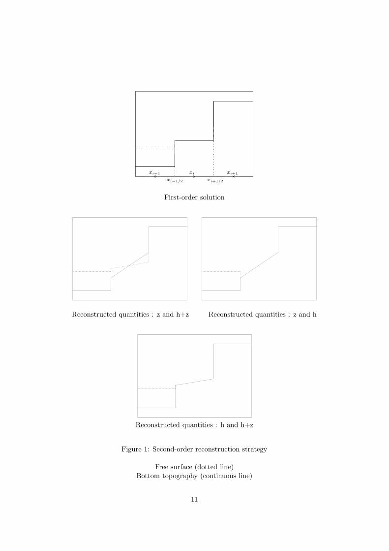
First, the cell by cell reconstruction preserves the mass conservation property of the finite vol-ume method. Second, the limitation procedure ensures the nonnegativity of the second-orderreconstructed water heights. The third important point is that the second-order reconstruc-tion has to preserve the lake at rest steady state. To ensure this property we reconstructalso the bottom topography z(x) although it is a data. The idea to do so is not so new -see [21], [11] - but here we give details on the more stable way to do it. Indeed only twoof the three quantities h, z, h + z need be explicitly reconstructed, the last being necessar-ily a combination of the other two. This is consistent with the strategy for second orderextensions of a well-balanced Godunov-type scheme for multi-dimensional compressible flow

9

under gravity in [5, 6], in that the deviations from the non-constant steady state form thebasis for reconstruction and slope limiting. A critical test to make the right choice is givenby considering a lake at rest with non vertical shores, that is nothing else but consideringan interface between a wet cell and a dry cell in the case where the bottom of the dry cellis higher than the free surface in the wet cell and where the fluid is at rest in the wet cell.As it appears in Figure 1, for the minmod reconstruction, the only choice which preservesthe steady state - or even the nonnegativity of water height in the worst case, see the thirdsubfigure - is to work with the quantities h and h + z. Notice that it follows that in somerespect the bottom topography changes at each timestep. It is obvious then that the chosensecond-order reconstruction preserves also the steady state in the classical case of wet-wetinterfaces since we explicitly reconstruct the quantity h + z. The second-order-centered con-dition (3.11) can be realized with a second-order ENO reconstruction for example, but inpractice we shall not do so because it becomes too complicate for 2d unstructured meshes,even if it necessarily means a slight loss of accuracy.

4 Numerical results

All numerical tests are computed with a kinetic solver. This solver is based on the kinetictheory developed in [25] and has the advantage - in the homogeneous case - to keep the waterheight nonnegative, to verify a discrete in-cell entropy inequality and to be able to computeproblems with shocks or vacuum.

4.1 1d assessments

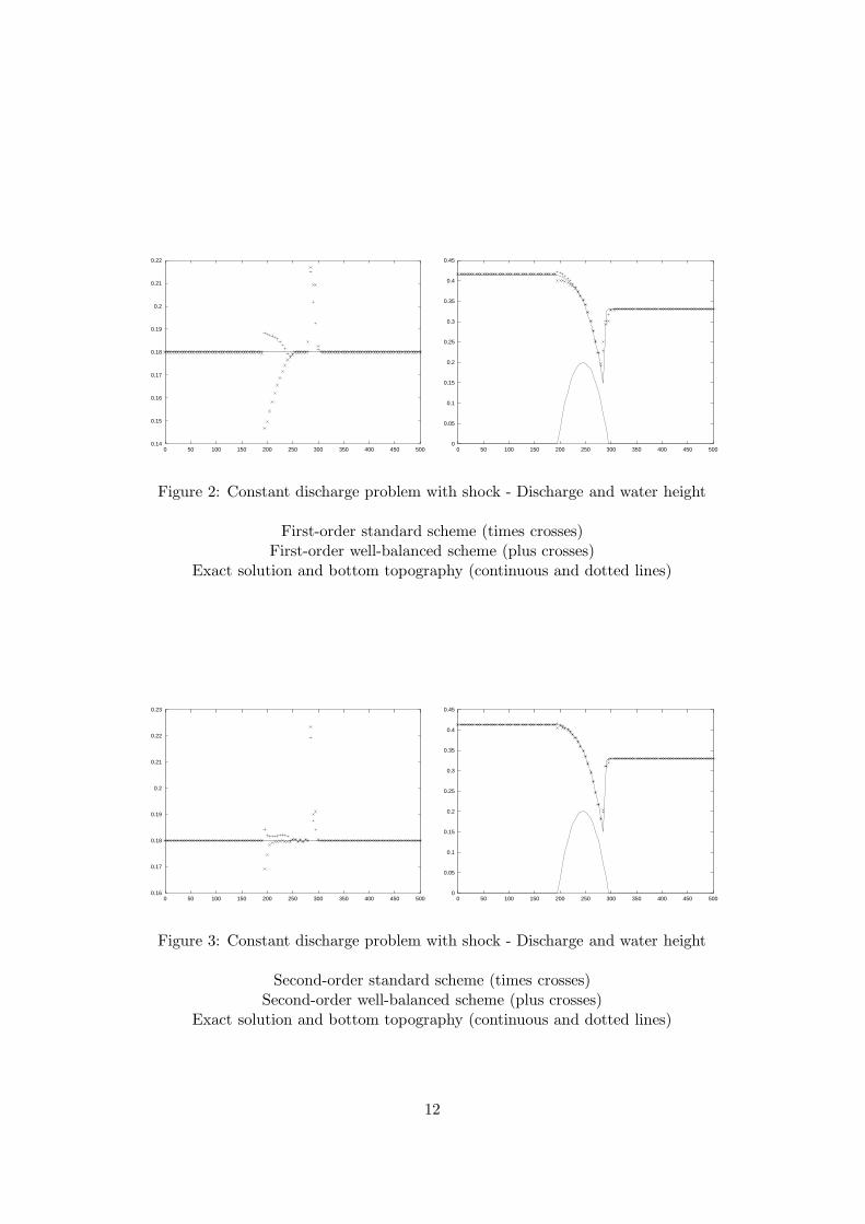
We first illustrate that the hydrostatic reconstruction does not affect the robustness of thehomogeneous solver. We present a very classical numerical test of a constant discharge tran-scritical flow with shock over a bump - refer to [15] for a complete presentation. In Figure3, where 101 points are used, we observe good first and second-order results for this testthe stiffness of which is well-known. As we are far from a hydrostatic steady state the re-sults of the well-balanced and standard schemes are quite similar. Notice however that thewell-balanced version is less affected - whatever is the order of resolution - than the standardscheme where the derivative of the bottom topography presents strong variations.

To exhibit the improvement due to the hydrostatic reconstruction we present now a quasi sta-tionary case first proposed by Leveque in [23] which consists in computing small perturbationsof the steady state of a lake at rest with a varying bottom topography,

z(x) = (0.25 (cos (π(x − 1.5)/0.1) + 1))+ ,

h(0, x) = 1. + 0.0011I[1.1,1.2].

As we can see by considering the linearized equations, the small perturbation simply moveto the right with a speed equal to

√h(t, x) i.e.

√1 − z(x) at first-order approximation - the

gravity is equal to one. We present in Figure 4 the results obtained - at t = 0.7s and with150 points - with the well-balanced scheme - on the right - and with the standard one - on

10

xixi−1

xi+1/2

xi+1

xi−1/2

First-order solution

Reconstructed quantities : z and h+z Reconstructed quantities : z and h

Reconstructed quantities : h and h+z

Figure 1: Second-order reconstruction strategy

Free surface (dotted line)Bottom topography (continuous line)

11

0.14

0.15

0.16

0.17

0.18

0.19

0.2

0.21

0.22

0 50 100 150 200 250 300 350 400 450 5000

0.05

0.1

0.15

0.2

0.25

0.3

0.35

0.4

0.45

0 50 100 150 200 250 300 350 400 450 500

Figure 2: Constant discharge problem with shock - Discharge and water height

First-order standard scheme (times crosses)First-order well-balanced scheme (plus crosses)

Exact solution and bottom topography (continuous and dotted lines)

0.16

0.17

0.18

0.19

0.2

0.21

0.22

0.23

0 50 100 150 200 250 300 350 400 450 5000

0.05

0.1

0.15

0.2

0.25

0.3

0.35

0.4

0.45

0 50 100 150 200 250 300 350 400 450 500

Figure 3: Constant discharge problem with shock - Discharge and water height

Second-order standard scheme (times crosses)Second-order well-balanced scheme (plus crosses)

Exact solution and bottom topography (continuous and dotted lines)

12

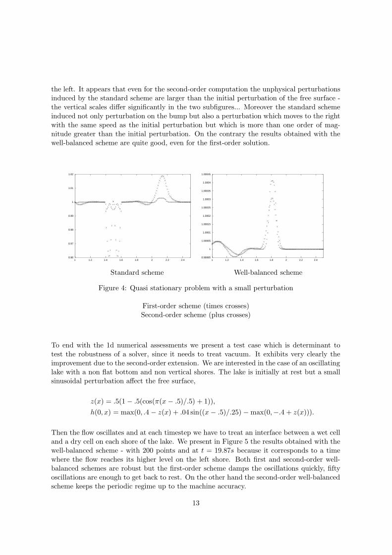
the left. It appears that even for the second-order computation the unphysical perturbationsinduced by the standard scheme are larger than the initial perturbation of the free surface -the vertical scales differ significantly in the two subfigures... Moreover the standard schemeinduced not only perturbation on the bump but also a perturbation which moves to the rightwith the same speed as the initial perturbation but which is more than one order of mag-nitude greater than the initial perturbation. On the contrary the results obtained with thewell-balanced scheme are quite good, even for the first-order solution.

0.96

0.97

0.98

0.99

1

1.01

1.02

1 1.2 1.4 1.6 1.8 2 2.2 2.40.99995

1

1.00005

1.0001

1.00015

1.0002

1.00025

1.0003

1.00035

1.0004

1.00045

1 1.2 1.4 1.6 1.8 2 2.2 2.4

Standard scheme Well-balanced scheme

Figure 4: Quasi stationary problem with a small perturbation

First-order scheme (times crosses)Second-order scheme (plus crosses)

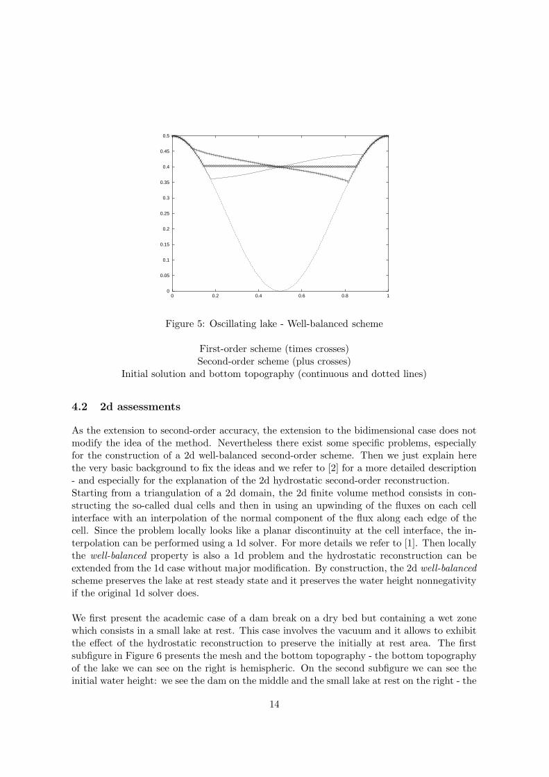
To end with the 1d numerical assessments we present a test case which is determinant totest the robustness of a solver, since it needs to treat vacuum. It exhibits very clearly theimprovement due to the second-order extension. We are interested in the case of an oscillatinglake with a non flat bottom and non vertical shores. The lake is initially at rest but a smallsinusoidal perturbation affect the free surface,

z(x) = .5(1 − .5(cos(π(x − .5)/.5) + 1)),

h(0, x) = max(0, .4 − z(x) + .04 sin((x − .5)/.25) − max(0,−.4 + z(x))).

Then the flow oscillates and at each timestep we have to treat an interface between a wet celland a dry cell on each shore of the lake. We present in Figure 5 the results obtained with thewell-balanced scheme - with 200 points and at t = 19.87s because it corresponds to a timewhere the flow reaches its higher level on the left shore. Both first and second-order well-balanced schemes are robust but the first-order scheme damps the oscillations quickly, fiftyoscillations are enough to get back to rest. On the other hand the second-order well-balancedscheme keeps the periodic regime up to the machine accuracy.

13

0

0.05

0.1

0.15

0.2

0.25

0.3

0.35

0.4

0.45

0.5

0 0.2 0.4 0.6 0.8 1

Figure 5: Oscillating lake - Well-balanced scheme

First-order scheme (times crosses)Second-order scheme (plus crosses)

Initial solution and bottom topography (continuous and dotted lines)

4.2 2d assessments

As the extension to second-order accuracy, the extension to the bidimensional case does notmodify the idea of the method. Nevertheless there exist some specific problems, especiallyfor the construction of a 2d well-balanced second-order scheme. Then we just explain herethe very basic background to fix the ideas and we refer to [2] for a more detailed description- and especially for the explanation of the 2d hydrostatic second-order reconstruction.Starting from a triangulation of a 2d domain, the 2d finite volume method consists in con-structing the so-called dual cells and then in using an upwinding of the fluxes on each cellinterface with an interpolation of the normal component of the flux along each edge of thecell. Since the problem locally looks like a planar discontinuity at the cell interface, the in-terpolation can be performed using a 1d solver. For more details we refer to [1]. Then locallythe well-balanced property is also a 1d problem and the hydrostatic reconstruction can beextended from the 1d case without major modification. By construction, the 2d well-balancedscheme preserves the lake at rest steady state and it preserves the water height nonnegativityif the original 1d solver does.

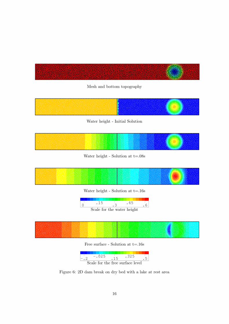
We first present the academic case of a dam break on a dry bed but containing a wet zonewhich consists in a small lake at rest. This case involves the vacuum and it allows to exhibitthe effect of the hydrostatic reconstruction to preserve the initially at rest area. The firstsubfigure in Figure 6 presents the mesh and the bottom topography - the bottom topographyof the lake we can see on the right is hemispheric. On the second subfigure we can see theinitial water height: we see the dam on the middle and the small lake at rest on the right - the

14

free surface level in the lake coincides with the reference level of the bottom topography ofthe river, i.e. (h + z)(0, x, y) = 0 everywhere on the right of the dam. On the third subfigurewe can see the rarefaction wave. Since it does not yet reach the lake, the steady state ispreserved. Then on the fourth subfigure the rarefaction wave reaches the lake and the waterbegins to move. On the last subfigure is presented the free surface level at this final time.We can notice strong variations on the lake area which lead to the formation of a hole - inthe left part of the lake, in blue on the subfigure - and a bump - in the right part, in greenin the subfigure - in the free surface.

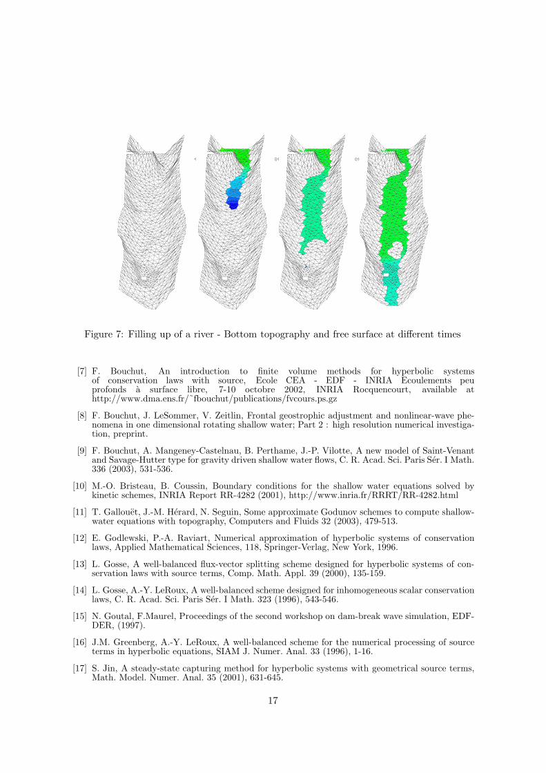
Then we present in Figure 7 another 2d numerical test corresponding to the filling up ofa river. This test still involves vacuum but also deals with complex realistic geometry andbottom topography since it takes into account a jetty in the transversal direction - on theupper part of the figures, a bridge pillar - the square on the lower part - and a small bump inthe bottom topography. We start with an empty river and we prescribe a given water levelas inflow condition. On the first subfigure are presented the mesh and the associated bottomtopography. Then we can notice that the strong variations in the bottom topography due tothe jetty or the pillar bridge does not affect the robustness of the computation. On the thirdand fourth subfigures we can see the bump since the water skirts it.

More results can be found in [1], [10], [26], [24], and in [8] with Coriolis force.

Acknowledgements

This work was partially supported by the ACI Modelisation de processus hydrauliques asurface libre en presence de singularites (http://www-rocq.inria.fr/m3n/CatNat/), by HYKEEuropean programme HPRN-CT-2002-00282 (http://www.hyke.org), by EDF/LNHE (E.A.,F.B., M.-O.B., B.P.), and by grant KL 611/6 of the Deutsche Forschungsgemeinschaft (R.K.).

References

[1] E. Audusse, M.-O. Bristeau, B. Perthame, Kinetic schemes for Saint-Venant equa-tions with source terms on unstructured grids, INRIA Report RR-3989 (2000),http://www.inria.fr/RRRT/RR-3989.html

[2] E. Audusse, M.-O. Bristeau, B. Perthame, Second order kinetic scheme for Saint-Venant equa-tions with source terms on unstructured grids, preprint.

[3] D.S. Bale, R.J. Leveque, S. Mitran, J.A. Rossmanith, A wave propagation method for conser-vation laws and balance laws with spatially varying flux functions, SIAM J. Sci. Comput. 24(2002), 955-978.

[4] R. Botchorishvili, B. Perthame, A. Vasseur, Equilibrium schemes for scalar conservation lawswith stiff sources, Math. Comp. 72 (2003), 131-157.

[5] N. Botta, R. Klein, S. Langenberg, S. Lutzenkirchen, Well-balanced finite volume methods fornearly hydrostatic flows, submitted to J. Comp. Phys., March (2002).

[6] N. Botta, R. Klein, A. Owinoh, Distinguished Limits, Multiple Scales Asymptotics, and Numericsfor Atmospheric Flows, Amer. Meteorological Society, 13th Intl. Conf. on Atmosphere-OceanFluid Dynamics, Breckenridge, Colorado, July (2001)

15

Mesh and bottom topography

INRIA-MODULEF

INRIA-MODULEF

INRIA-MODULEF

INRIA-MODULEF

0 .15

.3.45

.60 .15

.3.45

.6

Water height - Initial Solution

INRIA-MODULEF

INRIA-MODULEF

INRIA-MODULEF

INRIA-MODULEF

0 .15

.3.45

.60 .15

.3.45

.6

Water height - Solution at t=.08s

INRIA-MODULEF

INRIA-MODULEF

INRIA-MODULEF

INRIA-MODULEF

0 .15

.3.45

.60 .15

.3.45

.6

Water height - Solution at t=.16s

INRIA-MODULEF

INRIA-MODULEF

INRIA-MODULEF

INRIA-MODULEF

0 .15

.3.45

.60 .15

.3.45

.6Scale for the water height

INRIA-MODULEF

INRIA-MODULEF

INRIA-MODULEF

INRIA-MODULEF

-.2-.025

.15.325

.5-.2-.025

.15.325

.5

Free surface - Solution at t=.16s

INRIA-MODULEF

INRIA-MODULEF

INRIA-MODULEF

INRIA-MODULEF

-.2-.025

.15.325

.5-.2-.025

.15.325

.5Scale for the free surface level

Figure 6: 2D dam break on dry bed with a lake at rest area

16

INRIA-MODULEF

INRIA-MODULEF

INRIA-MODULEF

INRIA-MODULEF

252253

254255

256252253

254255

256INRIA-MODULEF

INRIA-MODULEF

INRIA-MODULEF

INRIA-MODULEF

252253

254255

256252253

254255

256INRIA-MODULEF

INRIA-MODULEF

INRIA-MODULEF

INRIA-MODULEF

252253

254255

256252253

254255

256INRIA-MODULEF

INRIA-MODULEF

INRIA-MODULEF

INRIA-MODULEF

252253

254255

256252253

254255

256Figure 7: Filling up of a river - Bottom topography and free surface at different times

[7] F. Bouchut, An introduction to finite volume methods for hyperbolic systemsof conservation laws with source, Ecole CEA - EDF - INRIA Ecoulements peuprofonds a surface libre, 7-10 octobre 2002, INRIA Rocquencourt, available athttp://www.dma.ens.fr/˜fbouchut/publications/fvcours.ps.gz

[8] F. Bouchut, J. LeSommer, V. Zeitlin, Frontal geostrophic adjustment and nonlinear-wave phe-nomena in one dimensional rotating shallow water; Part 2 : high resolution numerical investiga-tion, preprint.

[9] F. Bouchut, A. Mangeney-Castelnau, B. Perthame, J.-P. Vilotte, A new model of Saint-Venantand Savage-Hutter type for gravity driven shallow water flows, C. R. Acad. Sci. Paris Ser. I Math.336 (2003), 531-536.

[10] M.-O. Bristeau, B. Coussin, Boundary conditions for the shallow water equations solved bykinetic schemes, INRIA Report RR-4282 (2001), http://www.inria.fr/RRRT/RR-4282.html

[11] T. Gallouet, J.-M. Herard, N. Seguin, Some approximate Godunov schemes to compute shallow-water equations with topography, Computers and Fluids 32 (2003), 479-513.

[12] E. Godlewski, P.-A. Raviart, Numerical approximation of hyperbolic systems of conservationlaws, Applied Mathematical Sciences, 118, Springer-Verlag, New York, 1996.

[13] L. Gosse, A well-balanced flux-vector splitting scheme designed for hyperbolic systems of con-servation laws with source terms, Comp. Math. Appl. 39 (2000), 135-159.

[14] L. Gosse, A.-Y. LeRoux, A well-balanced scheme designed for inhomogeneous scalar conservationlaws, C. R. Acad. Sci. Paris Ser. I Math. 323 (1996), 543-546.

[15] N. Goutal, F.Maurel, Proceedings of the second workshop on dam-break wave simulation, EDF-DER, (1997).

[16] J.M. Greenberg, A.-Y. LeRoux, A well-balanced scheme for the numerical processing of sourceterms in hyperbolic equations, SIAM J. Numer. Anal. 33 (1996), 1-16.

[17] S. Jin, A steady-state capturing method for hyperbolic systems with geometrical source terms,Math. Model. Numer. Anal. 35 (2001), 631-645.

17

[18] T. Katsaounis, C. Simeoni, First and second order error estimates for the Upwind InterfaceSource method, preprint.

[19] T. Katsaounis, B. Perthame, C. Simeoni, Upwinding Sources at Interfaces in conservation laws,to appear in Appl. Math. Lett. (2003).

[20] A.-Y. LeRoux, Riemann solvers for some hyperbolic problems with a source term, ESAIM proc.6 (1999), 75-90.

[21] A.-Y. LeRoux, Discretisation des termes sources raides dans les problemes hyperboliques. In :Systemes hyperboliques : Nouveaux schemas et nouvelles applications. Ecoles CEA-EDF-INRIA’problemes non lineaires appliques’, INRIA Rocquencourt (France), March 1998 [in French].Available from http://www-gm3.univ-mrs.fr/˜leroux/publications/ay.le roux.html.

[22] R.J. LeVeque, Finite Volume Methods for Hyperbolic Problems, Cambridge University Press(2002).

[23] R.J. LeVeque, Balancing source terms and flux gradients in high-resolution Godunov methods:the quasi-steady wave-propagation algorithm, J. Comp. Phys. 146 (1998), 346-365.

[24] A. Mangeney, J.-P. Vilotte, M.-O. Bristeau, B. Perthame, C. Simeoni, S. Yernini, Numericalmodeling of avalanches based on Saint-Venant equations using a kinetic scheme, preprint 2002.

[25] B. Perthame, Kinetic formulations of conservation laws, Oxford University Press (2002).

[26] B. Perthame, C. Simeoni, A kinetic scheme for the Saint-Venant system with a source term,Calcolo 38 (2001), 201-231.

[27] B. Perthame, C. Simeoni, Convergence of the upwind Interface source method for hyperbolicconservation laws, to appear in Proc. of Hyp2002, T. Hou and E. Tadmor Editors.

[28] E.F. Toro, Riemann solvers and numerical methods for fluid dynamics. A practical introduction.Second edition. Springer-Verlag, Berlin, 1999.

[29] M.E. Vazquez-Cendon, Improved treatment of source terms in upwind schemes for the shallowwater equations in channels with irregular geometry, J. Comput. Phys. 148 (1999), 497-526.

[30] K. Xu, A well-balanced gas-kinetic scheme for the shallow water equations with source terms, J.Comput. Phys. 178(2) (2002), 533-562.

18