A Monitoring System for Online Fault Detection and

sensors

Article

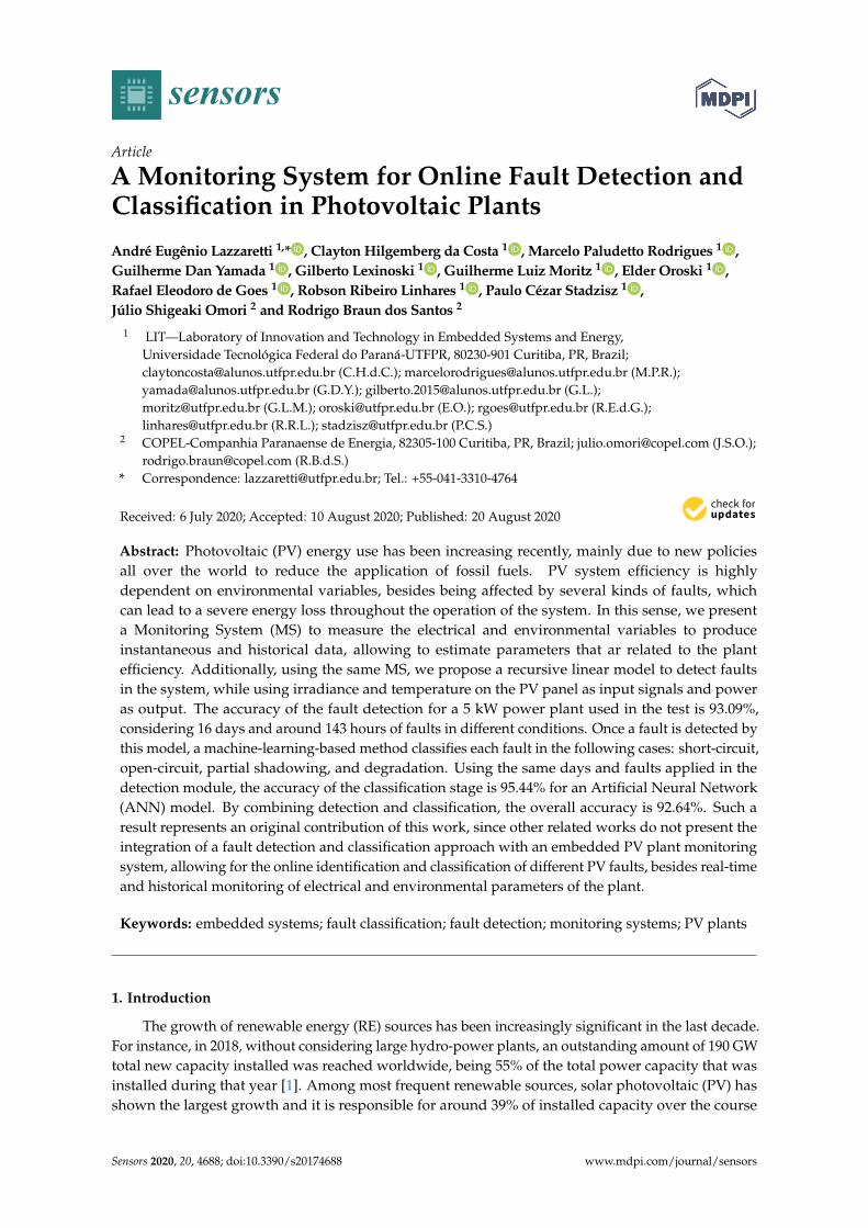
A Monitoring System for Online Fault Detection andClassification in Photovoltaic Plants

André Eugênio Lazzaretti 1,* , Clayton Hilgemberg da Costa 1 , Marcelo Paludetto Rodrigues 1 ,Guilherme Dan Yamada 1 , Gilberto Lexinoski 1 , Guilherme Luiz Moritz 1 , Elder Oroski 1 ,Rafael Eleodoro de Goes 1 , Robson Ribeiro Linhares 1 , Paulo Cézar Stadzisz 1 ,Júlio Shigeaki Omori 2 and Rodrigo Braun dos Santos 2

1 LIT—Laboratory of Innovation and Technology in Embedded Systems and Energy,Universidade Tecnológica Federal do Paraná-UTFPR, 80230-901 Curitiba, PR, Brazil;[email protected] (C.H.d.C.); [email protected] (M.P.R.);[email protected] (G.D.Y.); [email protected] (G.L.);[email protected] (G.L.M.); [email protected] (E.O.); [email protected] (R.E.d.G.);[email protected] (R.R.L.); [email protected] (P.C.S.)

2 COPEL-Companhia Paranaense de Energia, 82305-100 Curitiba, PR, Brazil; [email protected] (J.S.O.);[email protected] (R.B.d.S.)

* Correspondence: [email protected]; Tel.: +55-041-3310-4764

Received: 6 July 2020; Accepted: 10 August 2020; Published: 20 August 2020��

Abstract: Photovoltaic (PV) energy use has been increasing recently, mainly due to new policiesall over the world to reduce the application of fossil fuels. PV system efficiency is highlydependent on environmental variables, besides being affected by several kinds of faults, whichcan lead to a severe energy loss throughout the operation of the system. In this sense, we presenta Monitoring System (MS) to measure the electrical and environmental variables to produceinstantaneous and historical data, allowing to estimate parameters that ar related to the plantefficiency. Additionally, using the same MS, we propose a recursive linear model to detect faultsin the system, while using irradiance and temperature on the PV panel as input signals and poweras output. The accuracy of the fault detection for a 5 kW power plant used in the test is 93.09%,considering 16 days and around 143 hours of faults in different conditions. Once a fault is detected bythis model, a machine-learning-based method classifies each fault in the following cases: short-circuit,open-circuit, partial shadowing, and degradation. Using the same days and faults applied in thedetection module, the accuracy of the classification stage is 95.44% for an Artificial Neural Network(ANN) model. By combining detection and classification, the overall accuracy is 92.64%. Such aresult represents an original contribution of this work, since other related works do not present theintegration of a fault detection and classification approach with an embedded PV plant monitoringsystem, allowing for the online identification and classification of different PV faults, besides real-timeand historical monitoring of electrical and environmental parameters of the plant.

Keywords: embedded systems; fault classification; fault detection; monitoring systems; PV plants

1. Introduction

The growth of renewable energy (RE) sources has been increasingly significant in the last decade.For instance, in 2018, without considering large hydro-power plants, an outstanding amount of 190 GWtotal new capacity installed was reached worldwide, being 55% of the total power capacity that wasinstalled during that year [1]. Among most frequent renewable sources, solar photovoltaic (PV) hasshown the largest growth and it is responsible for around 39% of installed capacity over the course

Sensors 2020, 20, 4688; doi:10.3390/s20174688 www.mdpi.com/journal/sensors

http://www.mdpi.com/journal/sensors

http://www.mdpi.com

https://orcid.org/0000-0003-1861-3369

https://orcid.org/0000-0002-7117-1785

https://orcid.org/0000-0001-7409-8969

https://orcid.org/0000-0002-8998-5357

https://orcid.org/0000-0002-9617-0789

https://orcid.org/0000-0003-3628-2321

https://orcid.org/000-0003-3169-7245

https://orcid.org/0000-0002-8887-4145

https://orcid.org/0000-0002-4256-3819

https://orcid.org/0000-0003-2151-6754

http://www.mdpi.com/1424-8220/20/17/4688?type=check_update&version=1

http://dx.doi.org/10.3390/s20174688

http://www.mdpi.com/journal/sensors

Sensors 2020, 20, 4688 2 of 30

of 2018 [1]. Nevertheless, there are several performance issues that must be considered to increasePV performance. In the context of this work, for instance, PV performance can be compromised dueto the high exposure to different weather conditions, like soiling [2] and temperature [3], resulting inelectrical and mechanical faults, like cracked cells and short-circuits [4].

With such high exposure, the need of methods to maintain performance, reduce revenue lossesand downtime, and ensure rapid fault detection, classification, location, and mitigation in PV systemsemerge [5]. One way to achieve that is to include a MS in the PV plant that measures electricaland meteorological variables, manages plant operations (e.g., remote access), detects malfunctionsand errors, and reports performance and benchmarking, locally or remotely, through a communicationsystem to the grid operator [6,7]. However, only the MS is not enough to completely solve theproblem [8], since PV faults demand specific techniques to detect and classify them, using monitoreddata [9,10].

Techniques are normally divided into the detection and classification of PV faults, mainly focusedon the most recurrent ones, such as open-circuit, short-circuit, and module mismatch [11], in order toaccomplish those tasks. In terms of fault detection, there has been several proposals in the literature.In [12], for instance, fault detection that is based on satellite data is proposed. In other work [13],the PV module fault detection using thermal images allied with Canny edge detector is presented.Recently, several methods based on the modeling of PV systems have been proposed [14–16],achieving state-of-the-art results in real PV plants. However, such recent models are mostly basedon static models, discarding relevant dynamic modeling, and making it difficult to detect events thatoccur in short intervals of time [17].

In the fault classification context, there are different approaches, such as visual methods [18],thermographic image analysis methods [13], and mathematical methods using theoretical andsimulated models of PV plants [19]. More recently, some machine learning-based techniques havebeen proposed, improving the classification performance in different cases, mainly including theshadowing and degradation of PV modules [9,20,21]. Notwithstanding, most of the methods arefocused on simulated data and the authors do not present an extensive analysis of methods for onlinefault classification.

The limitations that are presented for detection and classification methods can be added to thefact that most of the models do not include results of the solution in a dedicated hardware or system,integrated to a monitoring system, and when they do, the PV plant power output is limited orthe detection can only be performed disturbing the normal operation of the system. In this sense,the main contribution of this work is the integration of a fault detection and classification approachwith an embedded PV plant monitoring system, allowing for non-intrusive online identification andclassification of different PV faults, besides providing a MS integrated to the plant. Additionally,we present a detailed comparison of dynamic models and machine learning approaches to detect andclassify, respectively, several real fault scenarios in a 5 kW PV plant, pointing to the most suitablemodel for online fault detection and classification in PV systems. To the extent of our knowledge,such a proposal has not yet been presented in the related literature.

This paper is organized, as follows. Section 2 addresses related works in terms ofmonitoring systems, fault detection and fault classification, together with a discussion regardingfaults in PV systems. Section 3 describes, in detail, the proposed monitoring system. Section 4 showsthe simulated and real datasets used to validate the detection and classification methods proposed inthis work. Sections 5 and 6 present theoretical and methodological aspects of the proposed detectionand classification methods, respectively. Section 7 presents the results of the monitoring system,detection, and classification approaches, comparing them with other related works. Finally, Section 8reports the general conclusions and suggests future research directions.

Sensors 2020, 20, 4688 3 of 30

2. Related Works

In order to present the main contributions of this work, we decided to divide the presentation ofrelated works into four main Subsections, which are the basis of this work. Initially, faults in PV systemsare discussed, emphasizing the most relevant faults and describing the characteristics of each fault.In the sequence, monitoring systems, fault detection, and fault classification are presented, showingthe main limitations observed in the recent literature. Finally, in Section 2.5, the original aspects ofthis work are detailed with respect to related monitoring systems, fault detection, and classificationmethods.

2.1. Faults in PV Systems

An important point for the evaluation of fault occurrence, as well as its impact, is the survey anddetails of, at least, the most common faults in photovoltaic systems. In this context, an extensive studyon those faults is presented in [22], dividing them into two categories: faults on the direct current(DC) side and faults on the alternating current (AC) side. Faults on the AC side are due to problemswith the inverter of the system or the power grid itself. Faults on the DC side are more numerousand they include: problems with the Maximum Power Point Tracking (MPPT) algorithm, faults inthe bypass diode, ground fault, arc faults, cell or module mismatch (which may be temporary orpermanent), open circuit, and short-circuit. In the context of this work, we selected the most recurrentfaults, which includes module mismatch, open-circuit, and short-circuit [11].

Open-circuit fault occurs when, at some point in the system, there is a disconnection, causing thecirculation of electrical current to be interrupted. From the power generation point of view, this faultis the one with the greatest impact [23], since it can affect from a single string of modules, up to theentire system, depending on the location of the disconnection and topology of the PV system.

The mismatch of cells or modules occurs when there are cells or modules in the PV systemwith electrical properties that are very different from the others, impairing their functioning [24].Mismatch fault can be divided into two subcategories: temporary and permanent. Temporary mismatchis normally caused by events, such as the deposition of dust or snow and by shadowing that is causedby buildings or transmission lines. The permanent mismatch occurs due to the degradation anddamage of the affected cells and modules. In the present work, both cases are taken into account,using shadowing and degradation as cases of temporary and permanent mismatch, respectively,both occurring at the module level.

The short-circuit fault occurs when a low impedance path appears along the system. In the caseof PV systems, this can occur at several points, such as between two terminals of the same module,two points of the same string, two different strings, and a string with the ground. In this work,the occurrence between two points of the same string will be taken into account, more particularlybetween the negative terminal of a module and the positive terminal of its adjacent module, which isgenerally the most impacting short-circuit fault from the energy production point of view.

2.2. Monitoring Systems

In grid-connected PV systems, which is the main focus of this work, the variables commonlymeasured to detect and classify faults are [19,23]: total irradiance; wind speed; wind direction;output voltage and current of each PV array; output power and energy of each PV array; ambienttemperature; PV module temperature; grid voltage; bidirectional current of the grid; bidirectionalpower; and, energy of the grid. Besides allowing the identification of faults in the components of theplant (modules, connection lines, converters, and inverters), these variables are the basis to enablethe evaluation of the plant performance in real-time and the improvement of the system reliability,as suggested in [25].

In this sense, several works have been proposed to present data acquisition systems in order tomeasure those variables. In [7], for instance, the data acquisition is composed of wireless sensors that

Sensors 2020, 20, 4688 4 of 30

are distributed around the plant, which measure electrical and meteorological parameters. The authorsanalyze the performance of the system in a 400 kW transformation center, presenting the results of thesensor network under different conditions of operation. However, fault detection and classificationare not discussed in that work, since the main contribution presented by authors is a high-precisionprotocol for synchronizing all data.

Still, in the context of wireless sensor networks (WSNs), a Zigbee (Zigbee is wirelesscommunication system based on the IEEE 802.15.4 specification for personal area networksusing low-power digital radios [26])-based online MS of a grid-connected utility-scale PV systemwas proposed in [27]. The system measures PV temperature, irradiation, and power output.Additionally, the authors present a web-application, similar to the solution proposed in [28], allowingfault detection and location in real-time. Nevertheless, a common limitation of those works is the highdependence on the correct functioning of the distributed sensors. The failure of one or more sensorscompromises the identification and location of faults throughout the plant.

Different approaches have been proposed with the aim of providing a low-cost sensor network fora massive monitoring in a PV plant, and avoiding the high dependence on individual sensors. In [6],for instance, a set of low-cost voltage, current, and temperature sensors was applied in the context ofdetecting critical faults, such as temporary and permanent shadowing, dirtying, and anomalous agingin a single PV panel. However, short-circuits and other types of faults are not discussed in that work.Besides, the proposed sensor network was installed in a single PV panel and it was not expanded to aPV plant.

Similarly, the development of low-cost sensors was proposed in [29,30], with the aim of obtainingthe lowest possible cost for monitoring electrical and temperature variables. Following a differentmethod for data transmission, but keeping the low-cost strategy, in [31], the PV panel’s voltage, current,and temperature were measured and transferred to the central control system using power lines carrierscommunications (PLC) technology on DC power lines. Similarly, in [32], a system composed of aWSN to obtain information of solar panels for timely repair and maintenance is presented, particularlydesigned for domestic applications. Nevertheless, because these works are mainly focused on low-costmonitoring systems, they do not present an analysis of faults and malfunctioning of the PV plant—i.e.,the use of monitored variables in the context of plant maintenance.

2.3. Fault Detection

In general, fault detection for PV systems is based on the modeling of the system in order tocompare the results from modeling with real-acquired data, indicating a fault event every time thedifference between modeling and acquired data is above some predefined threshold [16]. The modelingstep is normally divided into dynamic or static. Static models do not consider time as an independentvariable and, due to that, they are normally referred as non-memory models. Dynamic models, on theother hand, take time variations in the model into account. In PV modeling, static models are the mostrecurrent, in which PV cells are represented by the Single Diode Model [33].

In [5,34,35], a static model that is based on a single diode model is considered in the modelingprocess to detect faults and predict energy production. However, the main limitation of this group ofmodels is the representation of a generic and static PV cell. By simplifying the PV cell to a generic andstatic one, individual characteristics and the dynamics of different PV systems may be disregarded,compromising the modeling of certain phenomena and, consequently, the identification of faults thatoccur in short intervals of time. Nevertheless, from the diagnosis point of view, the static model isappropriate for detecting aging and degradation issues, due to the long-term characteristics of suchfaults [35].

In [14,15], a statistical approach based on the multivariate exponentially weighted moving averagecharts is proposed for fault detection in order to improve those limitations of single-diode models.The authors generated array’s residuals of DC current, voltage and power, considering temperatureand irradiance as inputs. With the residuals, it is possible to calculate the difference between the

Sensors 2020, 20, 4688 5 of 30

measurements and the predictions for the electrical variables from the single-diode model, and usethem as fault detectors. Real-acquired data show the ability of the proposed method to detectpartial shadowing, open-circuit, short-circuit, and degradation, but the authors only present sevencase-studies, which does not demonstrate the generalization of the model for other fault scenarios.Additionally, because the model is based on a decision-tree classifier, it is restricted to the presented9.6 kWp PV plant.

In terms of dynamic modeling, most of the models are dedicated to energy forecasting anddo not present fault detection results. In [16], for instance, a black-box modeling is used to obtainan empirical model for the system, using temperature and irradiance as input signals. However,that paper simplifies the model by excluding possible system nonlinearities, which makes it difficult touse in the context of fault detection. In [36], on the other hand, the Hammerstein–Wiener model isused to emulate the system including nonlinearities. The irradiance and DC power were used as inputand output signals, respectively. The chosen sampling time was 15 min., compromising the detectionof short-term events, such as partial shadowing. In [37], an ARMAX model is proposed to predictthe generated power, one-day ahead, for a PV system. The input signals of the ARMAX model arethe daily average temperature, the precipitation, the insulation duration, and the humidity. However,the authors did not discuss fault detection with the proposed model.

It is also noteworthy that none of the discussed detection methods presented the results of thesolution in a dedicated hardware or system, integrated to a monitoring system.

2.4. Fault Classification

One way to perform fault classification, which has been receiving increasing attention andpopularity in recent literature [9], is the use of artificial intelligence models, especially machinelearning classifiers, which is also the main approach that is proposed in this work. In [10], for instance,the use of artificial neural networks to classify the operation of a photovoltaic system in four possiblestates (normal, degradation, short-circuit, and shadowing) is presented. This method was trainedand tested in a simulated environment and obtained an accuracy of approximately 88.89% whenconsidering the nine evaluated test samples. Real fault cases were not reported in that work.

In [38], a two-stage system is discussed, being the first for fault detection and the second forclassification. The authors consider the following cases: open-circuit, degradation, short-circuit,and shadowing, including or not the bypass diode. For fault detection, the proposed method isbased on the comparison of the power of the PV plant with its correspondent mathematical model.When a difference above a given threshold is verified, the system reports a fault detection. For faultclassification, a multilayer perceptron artificial neural network is used, reaching an overall accuracy of90.3% (detection and classification). Furthermore, this system uses only simulated data for trainingthe network and it is tested with a real plant based on the system’s VxI curve. With that, the real-timeclassification of faults is unfeasible, since the generation of the VxI curve requires the disconnection ofthe plant to connect the proposed equipment and perform the detection and classification. Following asimilar idea, a detection and classification system is presented in [20], obtaining an accuracy of 94.1%.However, the authors also presented tests only in a simulation environment.

In a more recent approach from [39,40], another two stage architectures were used, but this timenon-linear auto regressive models (NARX) were developed to estimate the generated power underdifferent environmental conditions. Next, fuzzy inference models compared the estimated valueto the sensed power in order to classify the system into one of a given set of fault configurations,which includes combinations of shadowing, short circuit and open circuit, yielding 98.2% accuracy,using 16 use cases.

Still, in the context of intelligent methods in two stages, in [41,42], systems for detecting normal,open-circuit, and different types of short-circuits were proposed. The two-stage approach of theaforementioned works takes place with the use of probabilistic neural networks, for detection andclassification of the referred faults. In [41], two simulated tests were carried out to validate the proposed

Sensors 2020, 20, 4688 6 of 30

system, achieving a detection and classification accuracy of 82.34% and 98.19%, respectively while [42]achieves 100% accuracy while using real data for training and validation.

More specialized approaches use methods to detect line-to-line faults in several situations.For example, [43] uses a support vector machine trained with simulated data and tested in a real PVplant which achieves up to 94.74% accuracy to detect short-circuit conditions, while [44] uses a RadialBasis Function Neural Network using irradiance and power as its inputs to detect one or modulesdisconnections from the photovoltaic system. The system attained 98.1%, 97.9%, and 96.5% accuracywhen tested in two plants, one with 2.2 kW and other with 4.16 kW when subject to normal operation,shadowing, and overcast conditions. Another Radial Bases Function Network was used in [45] toclassify a 1 kW photovoltaic plant into one of 14 cases, including: Normal, short circuit, cell bypass,shading, ground fault, and nine converter/inverter’s component faults. This system was only testedin simulations and achieved 97% test accuracy.

In [11], on the other hand, a method using a Kernel Extreme Learning Machine and data fromVxI curves is presented in order to classify PV faults in the following cases: open-circuit, shadowing,short-circuit, and degradation. To evaluate the performance of the system, three case studies werecarried out. The first uses only simulation data for training and testing, whilst the second employsonly real data acquired in a 1.8 kW peak PV plant. The third approach uses simulated data fortraining and real data for testing, due to the limited amount of data collected in the real plant. In thecase that uses only simulated data, the proposed system reached an accuracy of 100.0%. In the casewith real data, the accuracy varied between 97.9% and 99.0% and, in the third case, with mixeddata, the final accuracy was 98.9%. Despite the relatively high performance (>95.0%), because themethod is based on VxI curves, the PV system must be disconnected to perform the proposed faultclassification procedure—it uses an external device that must be connected to the plant to obtain VxIcurves. Additionally, the authors did not present the results of the solution in a dedicated hardware orsystem.

2.5. Contributions of This Work

Based on the exposed so far, it can observed that fault detection and classification is a hot topicwith very interesting contributions so far. This work complements the current literature presentingdifferent contributions with respect to monitoring of PV systems, detection and classification of faults.In terms of monitoring systems, the related works show that, when the monitoring of plant variablesis more comprehensive, there is usually no fault analysis. On the other hand, when fault detectionis included (embedded) in the monitoring system, the detected faults are limited to certain typesof faults. When both are present, the work is only evaluated using simulations or with lower poweredPV deployments. With that, the first contribution of this work is the integration of a fault detectionand classification approach with an industrial grade embedded photovoltaic plant monitoring system,allowing for the online identification and classification of different PV faults, besides providing a MSintegrated to the plant.

Regarding the fault detection, the use and a very detailed comparison of dynamic models forseveral fault scenarios is still limited in the literature and it can be highlighted as an additionalcontribution of this work, particularly for real-acquired data. Finally, from the classification pointof view, the use of simulated (and validated) data to train machine learning models with differentfault conditions, besides testing with several real-acquired data in real fault scenarios, is also brieflyevaluated in the literature and can be highlighted as a relevant contribution. Besides, we also present adetailed comparison among some of the most common machine learning methods, pointing to themost suitable model for online fault classification in PV systems.

Another relevant contribution of our work is the fact that the simulator and the training dataset ispublicly available to enable straightforward comparison with newly proposed techniques.

Sensors 2020, 20, 4688 7 of 30

Finally, it is worth mentioning that this work is an extension and combination of previousworks [8,17,21] of the authors of this paper, which presented initial and individual results of monitoringsystem, fault detection, and classification, respectively.

3. Proposed Monitoring System

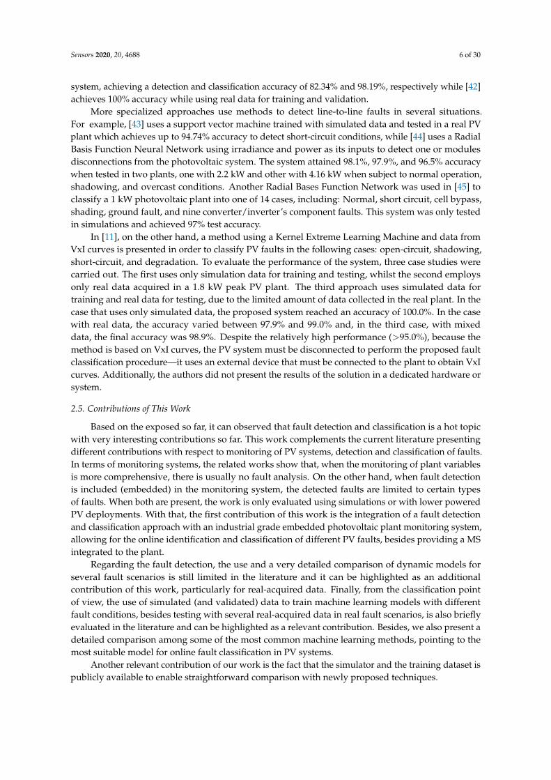
Suppose a photovoltaic system composed of a group S of strings each composed of N seriallyconnected photovoltaic modules PV{1, ... ,N}. When an arbitrary string s, (s ∈ S) is subject to anIrradiance (G), it generates a voltage Vdc , s and a current Idc , s (and, consequently, and output powerPdc , s = Vdc,s Idc,s), which are dependent on the ambient temperature T, considered constant for PVj,∀ j . An inverter is deployed to convert the energy output of the mentioned S string group into atwo-phase ac waveform whose voltage is Vac and current is Iac. The converted power is injected tothe utility grid. A data acquisition system is able to collect all of the aforementioned variables with aminimum sample frequency of 1 Hz. The power output may be influenced by the following systemfaults: (i) short circuit between an arbitrary number of adjacent PVj, ... ,k modules, (ii) open circuitof any module string ∈ S, (iii) high resistance connection between any adjacent PVj,k module pair,and (iv) module output mismatch due to partial shadowing. We propose a Fault Detection systemwhich uses the acquired data to detect whether the considered system is operating under one of theproposed faults. When a fault is detected, the fault classification is performed by the appropriatedalgorithm and the result is informed to the user.

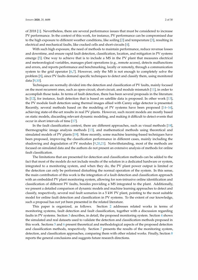
Figure 1 depicts the proposed system in which the acquisition system is implemented by aNational Instruments CompactRIO (cRIO) controller equipped with signal acquisition modules,as presented in Figure 2. The cRIO controller runs a Linux Real-Time Operating System and itfeatures a FPGA, and modular I/Os, programmed in the LabVIEW environment, for industrial-gradeembedded high-speed control and signal processing systems.

Two StringPV System

(5kW)

WeatherStation

Power Inverter

DataAcquisition

Fault Detection

Utility Grid

FaultClassification

Monitoring System

G, T

Vdc,s

Idc,s

Vac

Iac

Figure 1: The proposed method consists in transmitting a frame using ⌈α ncha⌉ channel uses for the first trans-mission attempt, with 0 < α ≤ 1. In the event of a decoding error, incremental redundancy is transmittedmaking use of the rest of the available ⌊(1 − α) ncha⌋ channel uses.

(a) (b) (c)

(d)(e)

(f) (g)


es(k), given by es(k) = pdc,s(k) − pdc,s(k)

2

Figure 1. General Overview of the System Model.

Sensors 2020, 20, 4688 8 of 30

Two StringPV System

(5kW)

WeatherStation

Power Inverter

DataAcquisition

Fault Detection

Utility Grid

FaultClassification

Monitoring System


(a) (b) (c)

(d)(e)

(f) (g)


1.1 Subsection Heading Here

Write your subsection text here.

2 Conclusion

Write your conclusion here.

2

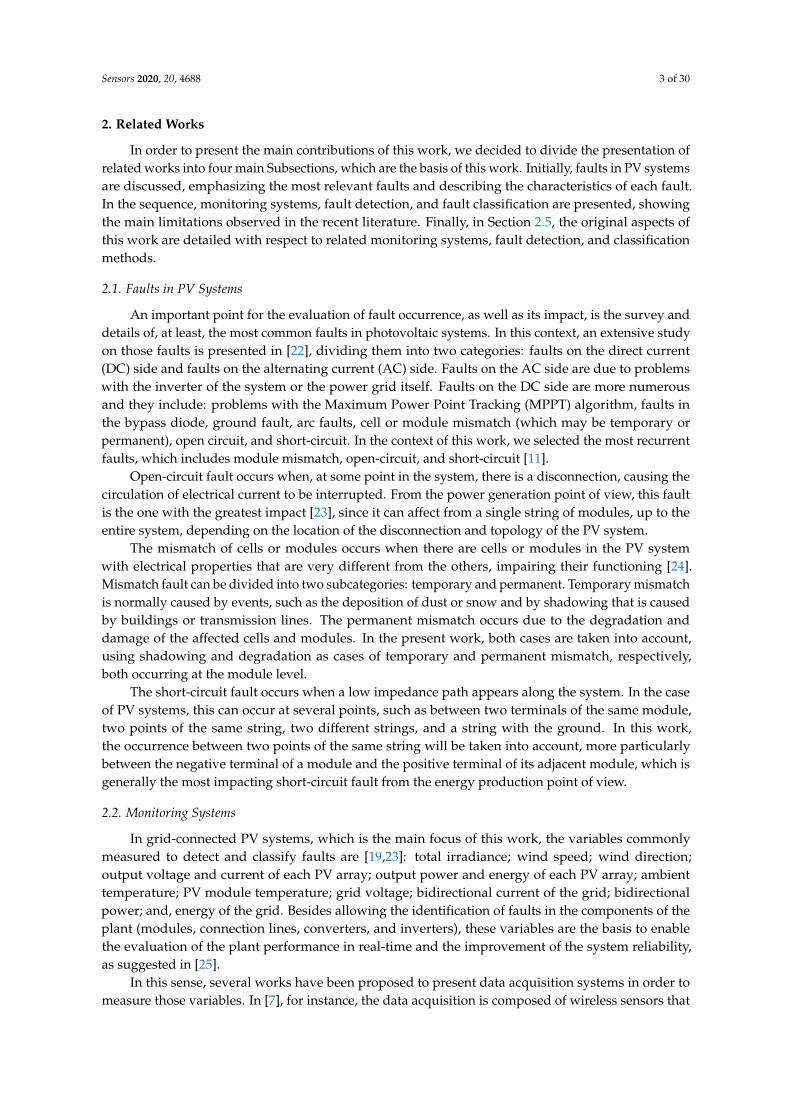
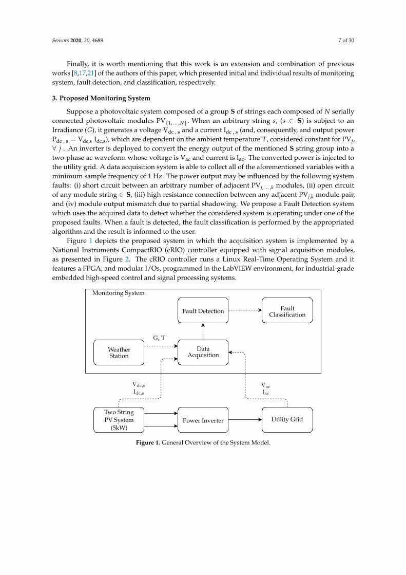
Figure 2. System Inside our Laboratory including: (a) Power Inverter, (b) Electrical Panel withProtection Devices and Signal Conditioning, (c) Local Display, (d) CompactRIO and Signal AcquisitionModules, (e) alternating current (AC) and direct current (DC) Current Transducers, (f) DegradationResistors, and (g) Power Quality Analyzer.

Between the acquired signals and the analysis, there is a software stack that comprises theexecution environment where the developed software coordinates the sampling at 25 kHz of Vdc,s,Idc,s, Vac, Iac, with s ∈ S. Next, the root mean square (RMS) values over the monitored variablesare calculated at every second, generating the signals vdc,s(k), idc,s(k),vac(k), iac(k) (with s ∈ S)which are stored on the local database. Additionally, RMS signals are calculated from themonitored signals: String power output pdc,s(k) = vdc,s(k) idc,s(k) and inverter power outputpac(k) = vac(k) iac(k). At the top of the stack, the fault detection and classification algorithmsare implemented. In the following subsections, the blocks from Figure 1 are presented.

3.1. PV Power Plant

In this work, PV{1, ... ,N} are implemented using N = 16, Canadian 330W Poly-crystalline Modules(CS6U-330P), forming a group S, with |S| = 2 strings of 8 modules each (where | · | representsgroup cardinality). Table 1 presents the main electrical data of the module.

Table 1. CS6U-330P Electrical Data.

DATA ValueOptimum Operating Voltage 37.2 V

Open Circuit Voltage 45.6 VOptimum Operation Current 8.88 A

Short Circuit Current 9.45 AModule Efficiency 16.97%

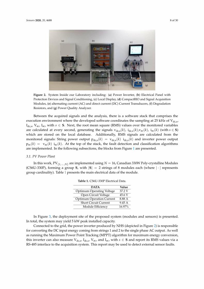
In Figure 3, the deployment site of the proposed system (modules and sensors) is presented.In total, the system may yield 5 kW peak installed capacity.

Connected to the grid, the power inverter produced by NHS (depicted in Figure 2) is responsiblefor converting the DC input energy coming from strings 1 and 2 to the single phase AC output. As wellas running the Maximum Power Point Tracking (MPPT) algorithm for maximum energy conversion,this inverter can also measure Vdc,s, Idc,s, Vac, and Iac, with s ∈ S and report its RMS values via aRS-485 interface to the acquisition system. This report may be used to detect external sensor faults.

Sensors 2020, 20, 4688 9 of 30

Figure 3: The proposed method consists in transmitting a frame using ⌈α ncha⌉ channel uses for the firsttransmission attempt, with 0 < α ≤ 1. In the event of a decoding error, incremental redundancy is transmittedmaking use of the rest of the available ⌊(1 − α) ncha⌋ channel uses.

String 1

String 2

ProtectionCircuit

ProtectionCircuit

HASS50S

HASS50S

PowerInverter

HASS50S

HASS50S

UtilityGrid

Signalconditioning

cRIO

NI 9216 NI 9215

RS-485

NI 9242

VDC,1

IDC,1

VDC,2

IDC,2

VAC,1

IAC,1

VAC,2

IAC,2


3

Figure 3. View of PV plant located at −25.438686 (Latitude) and −49.268487 (Longitude)–City ofCuritiba–State of Paraná–Brazil.

3.2. Weather Station

Because photovoltaic energy production is strongly dependent on the instantaneousenvironmental conditions where the solar panels operate, it is important for the acquisition system tocorrelate the instantaneous power output with meteorological variables. For this reason, a weatherstation was connected to cRIO to monitoring the variables that have the major influence in photovoltaicproduction: (i) irradiance G [W/m2]; and, (ii) module temperature T [◦C]. Additionally, our systemmeasures secondary variables that may influence the main variables: (iii) ambient temperature: Ta[◦C]; (iv) relative air humidity: H [%]; (v) dew point [◦C]; (vi) wind speed: Ws [m/s]; and, (vii) winddirection: Wd [degrees]. In Figure 3, the weather station may be observed adjacent to PV modulesand sensors.

For the irradiance (G) measurement, a EKO MS-40 class B pyranometer was installed adjacentto PV1 following the same inclination of the panel installation [19]. It is capable of measuring globalirradiance (285 to 3000 nm spectral sensitivity) with 180◦ angle. Panel temperature from PV{1, ... ,N} isassessed by four PT100 contact sensors, Kimo Instruments SFCSD-51-A-3-PVC-25, installed on theback side of PV1,6,11,16: T is considered to be the arithmetic average of the obtained measurements.The output accuracy of these sensors for temperatures between 0 and 100 ◦C is ±0.15 ◦C. Theenvironmental signals are obtained from a Novus Fieldlogger datalogger (eight analog input channels,with 24 bit A/D resolution and 1 kHz maximum sampling rate). The connection to the cRIO isimplemented through Modbus TCP/IP bus over ethernet. The datalogger is factory calibrated, so nofurther processing is necessary on the main monitoring system, besides synchronization and logging.The datalogger reports the 1 s average of G and T to the acquisition system, which are respectivelynamed g(k) and t(k) in the following sections.

3.3. Electrical Variables

Figure 4 shows a detailed view of the electrical variables acquisition scheme. There, the exactpoints of acquisition of monitored signals are indicated for DC voltage and current output for both PVstrings (Vdc,s, Idc,s with s ∈ S), as well as the AC voltage at the output of the power inverter (Vac, Iac),which are obtained by measuring both wires of the inverter with respect to the Utility Grid neutralwire (not shown for simplicity reasons) (Vac,1 , Iac,1, Vac,2, and Iac,2).

One NI 9215 module is used to acquire DC voltage signals of both strings. It reads twosimultaneously sampled analog input channels. Besides surge protection already installed in the

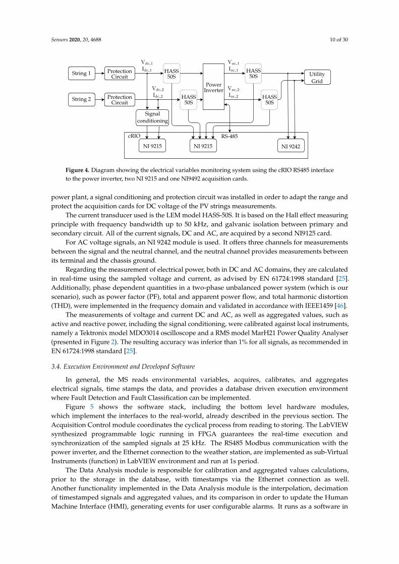
Sensors 2020, 20, 4688 10 of 30Figure 3: The proposed method consists in transmitting a frame using ⌈α ncha⌉ channel uses for the firsttransmission attempt, with 0 < α ≤ 1. In the event of a decoding error, incremental redundancy is transmittedmaking use of the rest of the available ⌊(1 − α) ncha⌋ channel uses.

String 1

String 2

ProtectionCircuit

ProtectionCircuit

HASS50S

HASS50S

PowerInverter

HASS50S

HASS50S

UtilityGrid

Signalconditioning

cRIO

NI 9215 NI 9215

RS-485

NI 9242

Vdc,1

Idc,1

Vdc,2

Idc,2

Vac,1

Iac,1

Vac,2

Iac,2


1.1 Subsection Heading Here

Write your subsection text here.

2 Conclusion

Write your conclusion here.

3

Figure 4. Diagram showing the electrical variables monitoring system using the cRIO RS485 interfaceto the power inverter, two NI 9215 and one NI9492 acquisition cards.

power plant, a signal conditioning and protection circuit was installed in order to adapt the range andprotect the acquisition cards for DC voltage of the PV strings measurements.

The current transducer used is the LEM model HASS-50S. It is based on the Hall effect measuringprinciple with frequency bandwidth up to 50 kHz, and galvanic isolation between primary andsecondary circuit. All of the current signals, DC and AC, are acquired by a second NI9125 card.

For AC voltage signals, an NI 9242 module is used. It offers three channels for measurementsbetween the signal and the neutral channel, and the neutral channel provides measurements betweenits terminal and the chassis ground.

Regarding the measurement of electrical power, both in DC and AC domains, they are calculatedin real-time using the sampled voltage and current, as advised by EN 61724:1998 standard [25].Additionally, phase dependent quantities in a two-phase unbalanced power system (which is ourscenario), such as power factor (PF), total and apparent power flow, and total harmonic distortion(THD), were implemented in the frequency domain and validated in accordance with IEEE1459 [46].

The measurements of voltage and current DC and AC, as well as aggregated values, such asactive and reactive power, including the signal conditioning, were calibrated against local instruments,namely a Tektronix model MDO3014 oscilloscope and a RMS model MarH21 Power Quality Analyser(presented in Figure 2). The resulting accuracy was inferior than 1% for all signals, as recommended inEN 61724:1998 standard [25].

3.4. Execution Environment and Developed Software

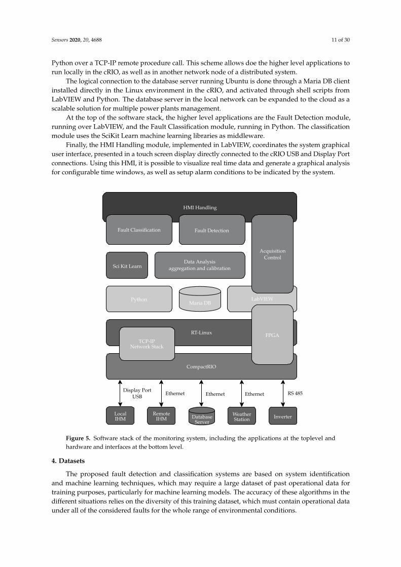
In general, the MS reads environmental variables, acquires, calibrates, and aggregateselectrical signals, time stamps the data, and provides a database driven execution environmentwhere Fault Detection and Fault Classification can be implemented.

Figure 5 shows the software stack, including the bottom level hardware modules,which implement the interfaces to the real-world, already described in the previous section. TheAcquisition Control module coordinates the cyclical process from reading to storing. The LabVIEWsynthesized programmable logic running in FPGA guarantees the real-time execution andsynchronization of the sampled signals at 25 kHz. The RS485 Modbus communication with thepower inverter, and the Ethernet connection to the weather station, are implemented as sub-VirtualInstruments (function) in LabVIEW environment and run at 1s period.

The Data Analysis module is responsible for calibration and aggregated values calculations,prior to the storage in the database, with timestamps via the Ethernet connection as well.Another functionality implemented in the Data Analysis module is the interpolation, decimationof timestamped signals and aggregated values, and its comparison in order to update the HumanMachine Interface (HMI), generating events for user configurable alarms. It runs as a software in

Sensors 2020, 20, 4688 11 of 30

Python over a TCP-IP remote procedure call. This scheme allows doe the higher level applications torun locally in the cRIO, as well as in another network node of a distributed system.

The logical connection to the database server running Ubuntu is done through a Maria DB clientinstalled directly in the Linux environment in the cRIO, and activated through shell scripts fromLabVIEW and Python. The database server in the local network can be expanded to the cloud as ascalable solution for multiple power plants management.

At the top of the software stack, the higher level applications are the Fault Detection module,running over LabVIEW, and the Fault Classification module, running in Python. The classificationmodule uses the SciKit Learn machine learning libraries as middleware.

Finally, the HMI Handling module, implemented in LabVIEW, coordinates the system graphicaluser interface, presented in a touch screen display directly connected to the cRIO USB and Display Portconnections. Using this HMI, it is possible to visualize real time data and generate a graphical analysisfor configurable time windows, as well as setup alarm conditions to be indicated by the system.

HMI Handling

Fault Classification Fault Detection

AcquisitionControl

Sci Kit LearnData Analysis

aggregation and calibration

PythonMaria DB

LabVIEW

FPGART-Linux

TCP-IPNetwork Stack

CompactRIO

Display PortUSB

Ethernet Ethernet Ethernet RS 485

LocalIHM

RemoteIHM Database

Server

WeatherStation Inverter


4

Figure 5. Software stack of the monitoring system, including the applications at the toplevel andhardware and interfaces at the bottom level.

4. Datasets

The proposed fault detection and classification systems are based on system identificationand machine learning techniques, which may require a large dataset of past operational data fortraining purposes, particularly for machine learning models. The accuracy of these algorithms in thedifferent situations relies on the diversity of this training dataset, which must contain operational dataunder all of the considered faults for the whole range of environmental conditions.

Sensors 2020, 20, 4688 12 of 30

We created a PV plant simulator that can generate the required dataset in a short period oftime since waiting for the natural occurrence of all these environmental combinations to generatethe required faults is impractical for most PV installations. On the other hand, the generated modelmust accurately describe a real system behavior. This way, we use the real photovoltaic installation(Section 3.1) to validate our simulator setup. This hybrid approach used to generate our training andvalidation dataset will be described in the following sections. First, the methodology to artificiallyintroduce operational faults in the real installation is described. In the sequence, the proposed electricalsimulator that matches the real installation behavior is presented.

4.1. Real System Installation

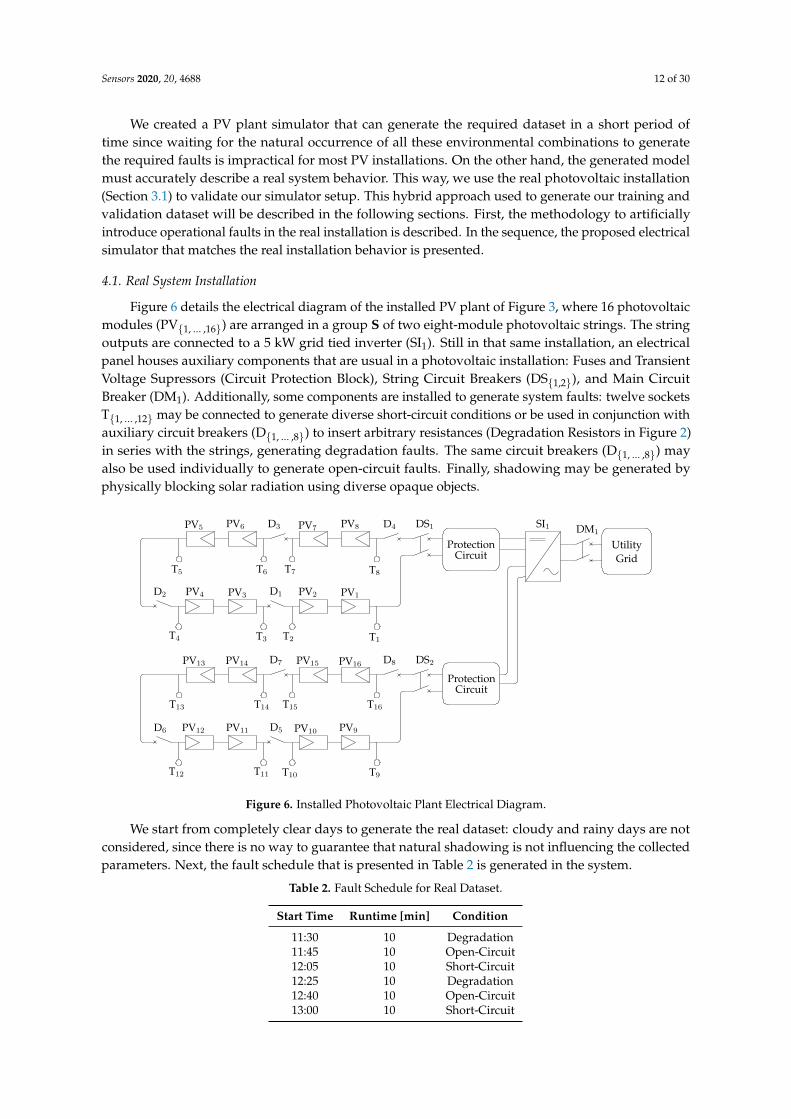
Figure 6 details the electrical diagram of the installed PV plant of Figure 3, where 16 photovoltaicmodules (PV{1, ... ,16}) are arranged in a group S of two eight-module photovoltaic strings. The stringoutputs are connected to a 5 kW grid tied inverter (SI1). Still in that same installation, an electricalpanel houses auxiliary components that are usual in a photovoltaic installation: Fuses and TransientVoltage Supressors (Circuit Protection Block), String Circuit Breakers (DS{1,2}), and Main CircuitBreaker (DM1). Additionally, some components are installed to generate system faults: twelve socketsT{1, ... ,12} may be connected to generate diverse short-circuit conditions or be used in conjunction withauxiliary circuit breakers (D{1, ... ,8}) to insert arbitrary resistances (Degradation Resistors in Figure 2)in series with the strings, generating degradation faults. The same circuit breakers (D{1, ... ,8}) mayalso be used individually to generate open-circuit faults. Finally, shadowing may be generated byphysically blocking solar radiation using diverse opaque objects.

PV1PV2PV3PV4

PV5 PV6 PV7 PV8

PV9PV10PV11PV12

PV13 PV14 PV15 PV16

T1T2T3T4

T5 T6 T7 T8

T9T10T11T12

T13 T14 T15 T16

D1D2

D3 D4

D5D6

D7 D8

DS1

DS2

ProtectionCircuit

ProtectionCircuit

SI1 DM1

UtilityGrid


+

-

Iph D Rp

Rs Ipv

Vpv


GT

VDC,1

IDC,1

VDC,2

IDC,2

D1

D2

VAC

IAC

S1

S2

B1

B2

J1


5

Figure 6. Installed Photovoltaic Plant Electrical Diagram.

We start from completely clear days to generate the real dataset: cloudy and rainy days are notconsidered, since there is no way to guarantee that natural shadowing is not influencing the collectedparameters. Next, the fault schedule that is presented in Table 2 is generated in the system.

Table 2. Fault Schedule for Real Dataset.

Start Time Runtime [min] Condition

11:30 10 Degradation11:45 10 Open-Circuit12:05 10 Short-Circuit12:25 10 Degradation12:40 10 Open-Circuit13:00 10 Short-Circuit

Sensors 2020, 20, 4688 13 of 30

Partial shadowing occurs naturally due to the characteristics of the deployment site: sunlight isblocked by a nearby buildings in different moments of the morning and afternoon (around two hoursin each period). The process was repeated for 16 days, when data is collected and properly labeledfrom around 07:30 to 17:00, including faults and normal conditions, with a sampling ratio of 1 Hz,generating 10,371 points with degradation, 5999 points with short-circuit, 6024 points with open-circuit,184,311 points with partial shadowing, and 309,253 points in which no faults were introduced. This realdataset is also publicly available (https://github.com/clayton-h-costa/pv_fault_dataset) in order tofacilitate other experiments regarding fault detection and classification methods.

4.2. System Simulation

One major concern taken into consideration, when our PV simulator was developed, is the abilityto represent different commercially available components used in PV plants. For validation purposes,the parameters that are chosen for Dataset generation match the ones from the available systemdescribed in Section 3.

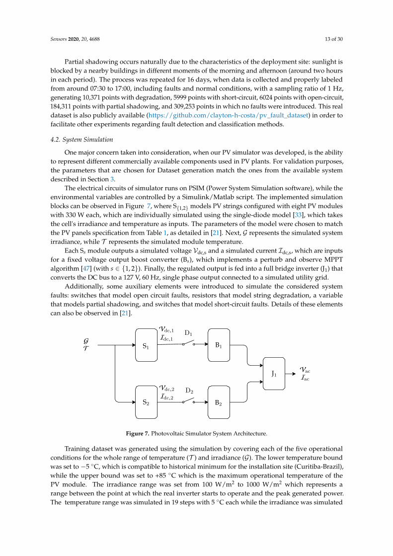
The electrical circuits of simulator runs on PSIM (Power System Simulation software), while theenvironmental variables are controlled by a Simulink/Matlab script. The implemented simulationblocks can be observed in Figure 7, where S{1,2} models PV strings configured with eight PV moduleswith 330 W each, which are individually simulated using the single-diode model [33], which takesthe cell's irradiance and temperature as inputs. The parameters of the model were chosen to matchthe PV panels specification from Table 1, as detailed in [21]. Next, G represents the simulated systemirradiance, while T represents the simulated module temperature.

Each Ss module outputs a simulated voltage Vdc,s and a simulated current Idc,s, which are inputsfor a fixed voltage output boost converter (Bs), which implements a perturb and observe MPPTalgorithm [47] (with s ∈ {1, 2}). Finally, the regulated output is fed into a full bridge inverter (J1) thatconverts the DC bus to a 127 V, 60 Hz, single phase output connected to a simulated utility grid.

Additionally, some auxiliary elements were introduced to simulate the considered systemfaults: switches that model open circuit faults, resistors that model string degradation, a variablethat models partial shadowing, and switches that model short-circuit faults. Details of these elementscan also be observed in [21].

y

PV1PV2PV3PV4

PV5 PV6 PV7 PV8

PV9PV10PV11PV12

PV13 PV14 PV15 PV16

T1T2T3T4

T5 T6 T7

T9T10T11T12

T13 T14 T15 T16

D1D2

D3 D4

D5D6

D7 D8

DS1

DS2

ProtectionCircuit

ProtectionCircuit

SI1 DM1

UtilityGrid


+

-

Iph D Rp

Rs Ipv

Vpv


GT

Vdc,1

Idc,1

Vdc,2

Idc,2

D1

D2

Vac

Iac

S1

S2

B1

B2

J1


5

Figure 7. Photovoltaic Simulator System Architecture.

Training dataset was generated using the simulation by covering each of the five operationalconditions for the whole range of temperature (T ) and irradiance (G). The lower temperature boundwas set to −5 ◦C, which is compatible to historical minimum for the installation site (Curitiba-Brazil),while the upper bound was set to +85 ◦C which is the maximum operational temperature of thePV module. The irradiance range was set from 100 W/m2 to 1000 W/m2 which represents arange between the point at which the real inverter starts to operate and the peak generated power.The temperature range was simulated in 19 steps with 5 ◦C each while the irradiance was simulated

https://github.com/clayton-h-costa/pv_fault_dataset

Sensors 2020, 20, 4688 14 of 30

in 19 steps of 50 W/m2 for each of the four considered faults. For the shadowing fault, four differentcases were simulated, each with a set amount of shade varying from 5% to 15% of a string, which isthe typical shadowing observed in the PV plant. This setup resulted in 361 sample cases per string,with 5054 samples in total.

5. Fault Detection

Fault detection technique, as expressed in this section, is based on modelling the photovoltaicsystem dynamics, and uses the matching between the real system and the model as a metric of properlyoperation of the system. In this context, it is important to clarify two concepts as: (i) system: defined asconfined arrangement of mutually affected entities [48]; and, (ii) model: defined as mathematicalrepresentation of these systems [49]. The next section will bring more details about the PVmodeling process.

5.1. System Identification Model

In this work, the methodology that was used to achieve proper models for real systems wasbased on system identification. In this context, one can define system identification as a method ofmeasuring the mathematical description of a system by processing the observed inputs and outputs ofthe system [50]. Generally, a model achieved by this technique is more accurate to describe a systemthan models based only on physical laws [48]. In the scenario of this work, it is possible to applymodels in order to detect miss-functions of an specific system [51].

It is important to mention that only the real dataset (detailed in Section 4.1) was employed inorder to estimate the detection model parameters.

5.2. Proposed Fault Detection Method

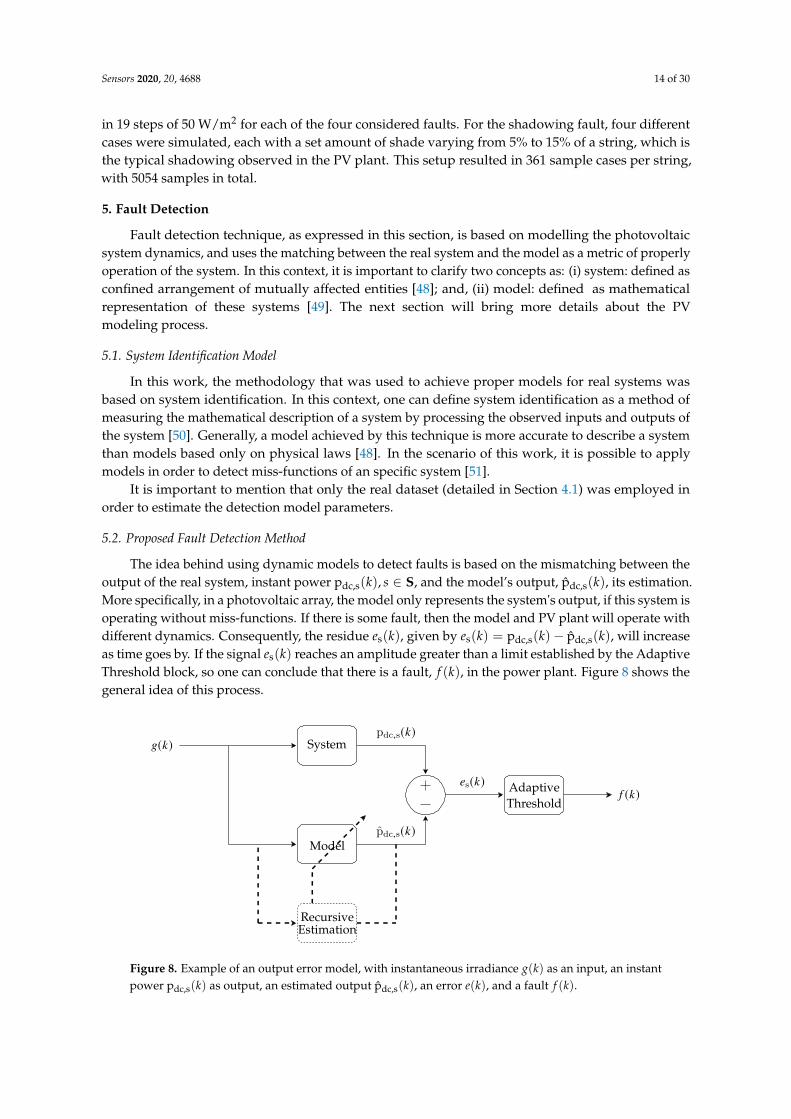
The idea behind using dynamic models to detect faults is based on the mismatching between theoutput of the real system, instant power pdc,s(k), s ∈ S, and the model’s output, pdc,s(k), its estimation.More specifically, in a photovoltaic array, the model only represents the system's output, if this system isoperating without miss-functions. If there is some fault, then the model and PV plant will operate withdifferent dynamics. Consequently, the residue es(k), given by es(k) = pdc,s(k)− pdc,s(k), will increaseas time goes by. If the signal es(k) reaches an amplitude greater than a limit established by the AdaptiveThreshold block, so one can conclude that there is a fault, f (k), in the power plant. Figure 8 shows thegeneral idea of this process.

g(k)pdc,s(k)

pdc,s(k)

es(k)f (k)

System

Model

RecursiveEstimation

AdaptiveThreshold


.

.

.

��

SimulatedData

Test(20%)

Train(80%)

Train(80%)

Test(20%)

Train(80%)

Train(80%)

Test(20%)

Train(80%)

Train(80%)

Test(20%)

Train(80%)

Train(80%)

Test(20%)

Mean Accuracy


6

Figure 8. Example of an output error model, with instantaneous irradiance g(k) as an input, an instantpower pdc,s(k) as output, an estimated output pdc,s(k), an error e(k), and a fault f (k).

Sensors 2020, 20, 4688 15 of 30

In this work, the dynamics of the underlying system was approximated by a linearAuto-Regressive with eXogenous input (ARX) model, expressed by

pdc,s(k) = a1 pdc,s(k− 1) + a2 pdc,s(k− 2) + b0 g(k) + b1 g(k− 1), (1)

or one can obtain the system’s transfer function, using z transform

P(z)G(z)

=b0 + b1 z−1

1− a1 z−1 − a2 z−2 , (2)

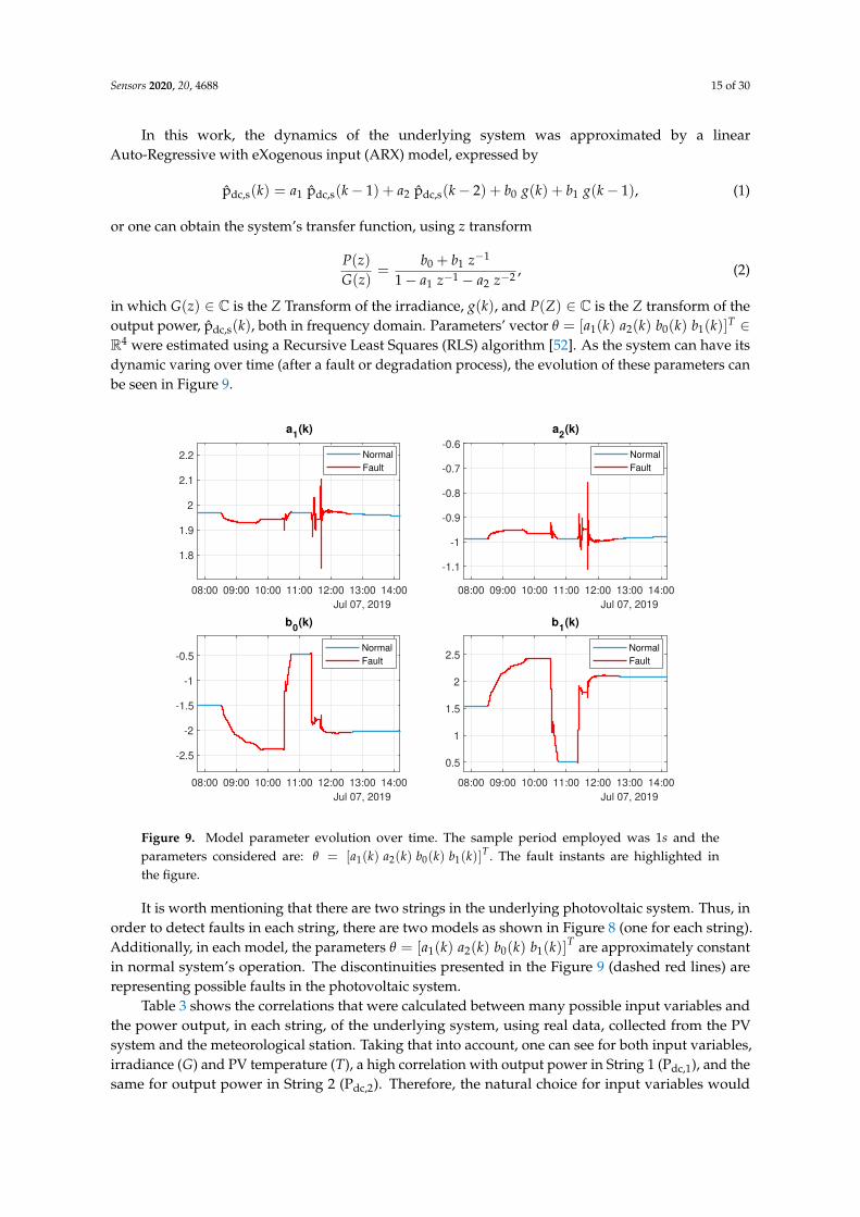
in which G(z) ∈ C is the Z Transform of the irradiance, g(k), and P(Z) ∈ C is the Z transform of theoutput power, pdc,s(k), both in frequency domain. Parameters’ vector θ = [a1(k) a2(k) b0(k) b1(k)]T ∈R4 were estimated using a Recursive Least Squares (RLS) algorithm [52]. As the system can have itsdynamic varing over time (after a fault or degradation process), the evolution of these parameters canbe seen in Figure 9.

08:00 09:00 10:00 11:00 12:00 13:00 14:00

Jul 07, 2019

1.8

1.9

2

2.1

2.2

a1(k)

Normal

Fault

08:00 09:00 10:00 11:00 12:00 13:00 14:00

Jul 07, 2019

-1.1

-1

-0.9

-0.8

-0.7

-0.6

a2(k)

Normal

Fault

08:00 09:00 10:00 11:00 12:00 13:00 14:00

Jul 07, 2019

-2.5

-2

-1.5

-1

-0.5

b0(k)

Normal

Fault

08:00 09:00 10:00 11:00 12:00 13:00 14:00

Jul 07, 2019

0.5

1

1.5

2

2.5

b1(k)

Normal

Fault


07:00 08:00 09:00 10:00 11:00 12:00 13:00 14:00 15:00 16:00 17:00 18:00

Apr 16, 2020

0

0.5

1

Fa

ult

a

bf(k)

ARX f(k)

07:00 08:00 09:00 10:00 11:00 12:00 13:00 14:00 15:00 16:00 17:00 18:00

Apr 16, 2020

0

0.5

1

Fa

ult

b

bf(k)

DDM f(k)

07:00 08:00 09:00 10:00 11:00 12:00 13:00 14:00 15:00 16:00 17:00 18:00

Apr 16, 2020

0

0.5

1

Fa

ult

c

bf(k)

SDM f(k)

07:00 08:00 09:00 10:00 11:00 12:00 13:00 14:00 15:00 16:00 17:00 18:00

Apr 16, 2020

0

0.5

1

Fa

ult

d

bf(k)

HWM f(k)


8

Figure 9. Model parameter evolution over time. The sample period employed was 1s and theparameters considered are: θ = [a1(k) a2(k) b0(k) b1(k)]

T . The fault instants are highlighted inthe figure.

It is worth mentioning that there are two strings in the underlying photovoltaic system. Thus, inorder to detect faults in each string, there are two models as shown in Figure 8 (one for each string).Additionally, in each model, the parameters θ = [a1(k) a2(k) b0(k) b1(k)]

T are approximately constantin normal system’s operation. The discontinuities presented in the Figure 9 (dashed red lines) arerepresenting possible faults in the photovoltaic system.

Table 3 shows the correlations that were calculated between many possible input variables andthe power output, in each string, of the underlying system, using real data, collected from the PVsystem and the meteorological station. Taking that into account, one can see for both input variables,irradiance (G) and PV temperature (T), a high correlation with output power in String 1 (Pdc,1), and thesame for output power in String 2 (Pdc,2). Therefore, the natural choice for input variables would

Sensors 2020, 20, 4688 16 of 30

be: (i) irradiance (T); and, (ii) PV temperature (T). However, for simplicity reasons, only the irradianceG was chosen as input variable, because of its higher correlation: 0.96.

Table 3. Correlation index between environmental variables with the power of each string.

Environmental Variables Power (Pdc,1) Power (Pdc,2)

Irradiance (G) 0.96 0.96PV Temperature (T) 0.86 0.86

Dew Point (D) 0.41 0.41Ambient Temperature (Ta) 0.38 0.37Relative Air Humidity (H) −0.28 −0.27

Wind speed (Ws) 0.28 0.28Wind direction (Wd) 0.02 0.02

Furthermore, the linear ARX model was chosen because of the following reasons:

• ARX linear models are one of the most simple dynamic systems. Thus, its computationalimplementation is less time consuming, which is ideal for the implementation of monitoringsystems in photovoltaic area;

• The ARX model represents a close approximation to the real system, as detailed in Section 7.

It is important to mention that the proposed model is not the only one. In a previous work,the authors have already investigated Diode Models and Hammerstein-Wiener models, applied to thesame problem [17]. The comparisons will be presented in Section 7.

In order to detect faults using the mismatch between the system and model, an adaptivethreshold was employed, as can be seen in Figure 8. This block was mathematically composedby a recursive mean, expressed in (3), and recursive variance, expressed in (4), both being modulatedby a forgetting factor λ [51]:

e(k) = λ e(k− 1) + (1− λ)e(k), (3)

σ2(k) =2 λ− 1

λσ2(k− 1) + (1− λ) [e(k)− e(k)] , (4)

in which e(k) ∈ R is the mean of residues, in instant k ∈ Z, λ ∈ [0, 1], and σ2(k) ∈ R is the variance ofthe residues. One event is considered as a fault if the absolute value of the residue, |e(k)|, overflows thethreshold e(k)±n

√σ2(k), i.e.:if |e(k)| > max

(|e(k)| ±n

√σ2(k)

), f (k) = 1 (fault);

otherwise, f (k) = 0 (normal operation);(5)

The selection of the value n was empirically done, aiming at minimizing Mean Square Error (MSE)between f (k) and a benchmark signal, b f (k) ∈ B = {0, 1}, expressing the evolution of manipulatedfaults over time. In other words, b f (k) = 0 defines that there is no fault in the system, while b f (k) = 1represents a manipulated fail occurring.

5.3. Detection Metrics

In order to quantify the results that were obtained by the fault detection process, some metricswere employed in this work. However, before defining performance metrics for this process, it isimportant to define the following concepts:

• TP (True Positive): it happens when the detection process points out a real fault, in thephotovoltaic system;

• TN (True Negative): it occurs when there is no fault in the photovoltaic system, and the faultdetection system confirms that;

Sensors 2020, 20, 4688 17 of 30

• FP (False Positive): it happens when the photovoltaic system presents no fault, and the faultdetection system points out a fault; and,

• FN (False Negative): it occurs when the photovoltaic system presents a fault and the detectionsystem does not signalize it.

Based on this, one can define the following performance metrics for the proposed faultdetection system:

• Accuracy (A): corresponds to the overall detection efficiency:

A =TP + TN

TP + TN + FP + FN; (6)

• Precision (P): stands for the rate between positives indicators:

P =TP

TP + FP; (7)

• Sensitivity (S): evaluates the efficiency of classifying correct detection:

S =TP

TP + FN; (8)

• Specificity (E ): evaluates how efficiently the classifier identifies incorrect detections:

E =TN

TN + FP. (9)

6. Fault Classification

Whenever a fault is detected at a given time ( f (k) = 1), the fault classification block is responsiblefor indicating to the user the most probable cause of the abnormal operation. For this task, we evaluatedthe accuracy of the four most common supervised machine learning methods. The variables that werechosen as the input for these algorithms are the ones that describe the behavior of the DC side of thePV plant, where the faults occur, forming a feature vector

FV(k) =[

g(k) t(k) vdc,1(k) vdc,2(k) idc,1(k) idc,2(k)]

. (10)

The classification system may be represented as a mapping function h : FV(k) → Ψ,where Ψ =

{Lshort, Lopen, Ldegradation, Lshadowing

}represents a group of the four considered faults.

Every considered method uses a training procedure to construct h. A brief description of each methodand the training procedure will be detailed in the next paragraphs.

The first method tested was k-Nearest Neighbors [53], in which the current feature vector of the PVplant is associated to the one in the training set which presents the most similar characteristics (closestin terms of Euclidean distance). This method is very simple to implement, but has an disadvantage ofrequiring the complete training set to perform the classification.

For this reason, a still simple but less memory intensive method was considered: DecisionTrees [53]. In this method, a tree structure is formed in which each class is contained in a leaf node.For classification, this tree is traversed from node to leaves, with each step being guided by binarydecisions based on different input features. As an advantage, the classification procedure is very simple,but the process of building an efficient unbiased decision tree is not always available. Furthermore,a slight change on classes may require a complete tree rebuild, which motivates the search for moreefficient classification algorithms.

Another widely used classification method is Support Vector Machines [54], which operatesby creating a multidimensional vector space in which each feature vector is represented as a point.

Sensors 2020, 20, 4688 18 of 30

The training procedure consists in determining an hyperplane mapped so that the examples of theseparate classes are divided by a margin that must be made as wide as possible. The solution for theproblem can be found with convex optimization techniques.

The last compared method was artificial neural networks, which consists of a parallel distributedsignal processor that have the capacity to store knowledge using a learning algorithm. In this work, weused the Multi-Layer Perceptron (MLP) network [53], which is a feedforward architecture, with just asingle hidden layer, an input layer, and the output layer, which corresponds to the assigned class (label).The learning process is based on the backpropagation algorithm [53], which basically consists in amethod to estimate the gradient of the training error cost function, along the layers of the network,allowing the use of a gradient descent-based method to optimize and estimate the parameters. All ofthe mentioned algorithms were trained using the procedure depicted in the next section.

6.1. Training Procedure

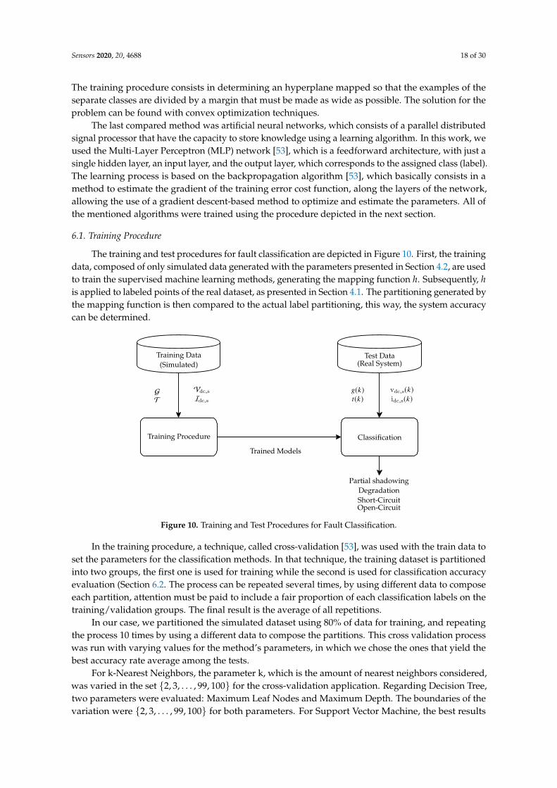
The training and test procedures for fault classification are depicted in Figure 10. First, the trainingdata, composed of only simulated data generated with the parameters presented in Section 4.2, are usedto train the supervised machine learning methods, generating the mapping function h. Subsequently, his applied to labeled points of the real dataset, as presented in Section 4.1. The partitioning generated bythe mapping function is then compared to the actual label partitioning, this way, the system accuracycan be determined.

1 1.2 1.4 1.6 1.8

105

1.7

1.8

1.9

2

2.1

2.2

a1(k)

1 1.2 1.4 1.6 1.8

105

-1.2

-1

-0.8

-0.6

-0.4

-0.2

a2(k)

1 1.2 1.4 1.6 1.8

105

-6

-4

-2

0

2

b0(k)

1 1.2 1.4 1.6 1.8

105

-2

0

2

4

6

b1(k)


Training Data(Simulated)

Training Procedure

Test Data(Real System)

Classification

GT

Vdc,s

Idc,s

Trained Models

g(k)t(k)

vdc,s(k)idc,s(k)

Partial shadowingDegradationShort-CircuitOpen-Circuit


8

Figure 10. Training and Test Procedures for Fault Classification.

In the training procedure, a technique, called cross-validation [53], was used with the train data toset the parameters for the classification methods. In that technique, the training dataset is partitionedinto two groups, the first one is used for training while the second is used for classification accuracyevaluation (Section 6.2. The process can be repeated several times, by using different data to composeeach partition, attention must be paid to include a fair proportion of each classification labels on thetraining/validation groups. The final result is the average of all repetitions.

In our case, we partitioned the simulated dataset using 80% of data for training, and repeatingthe process 10 times by using a different data to compose the partitions. This cross validation processwas run with varying values for the method’s parameters, in which we chose the ones that yield thebest accuracy rate average among the tests.

For k-Nearest Neighbors, the parameter k, which is the amount of nearest neighbors considered,was varied in the set {2, 3, . . . , 99, 100} for the cross-validation application. Regarding Decision Tree,two parameters were evaluated: Maximum Leaf Nodes and Maximum Depth. The boundaries of thevariation were {2, 3, . . . , 99, 100} for both parameters. For Support Vector Machine, the best results

Sensors 2020, 20, 4688 19 of 30

were achieved using the Gaussian kernel [54], which contains two parameters to be varied inthe cross-validation process: the regularization parameter C (searched in {0.5, 1, 2, 5, 10, 15, 20, 25}),which is responsible for the balance between model complexity and goodness of fit to the training dataand the kernel parameter γ (searched in {0.1, 0.5, 1, 2, 5, 10, 15, 20, 25}). Finally, the ANN was built withsix input units, four output units and a single hidden layer with its size as the sole hyperparameterused. The hidden layer uses the Rectified Linear Unit as activation function, while the output layeruses the softmax (normalized exponential function). Additionally, the optimization solver used wasthe Adaptive Moment Estimation, or ADAM, as presented in [55]. The search for the hidden layer size,via cross-validation, was made in the interval {5, 6, . . . , 29, 30} neurons.

6.2. Classification Metric

For overall performance assessment of the classification stage, one can construct a confusion matrixwith J classes, being J equals to the number of faults. Using this confusion matrix, the performance forall classes in terms of classification accuracy can be calculated, while using individual performances perclass. The individual performance is computed by the number of corrected classified examples dividedby the total number of examples per class. Subsequently, the average of individual performancesis used to reduce the impact of class imbalance on the final result, allowing for a more adequatecomparison among all methods.

7. Results and Discussion

In this section, all of the results are presented and discussed. First, the results of individualfault detection are presented, comparing recursive approaches and indicating the most appropriatemodel proposed in this work. In the sequence, the validation of simulated data for classification ispresented, in order to highlight the use of simulated data in the context of classification. Posteriorly,the results of individual fault classification are presented, for different machine learning models.Subsequently, a combination of the best fault detection and classification models is presented, followedby a comparison with state-of-the-art models. Finally, the results of the MS with integrated faultdetection and classification are depicted.

7.1. Fault Detection

7.1.1. Model Results

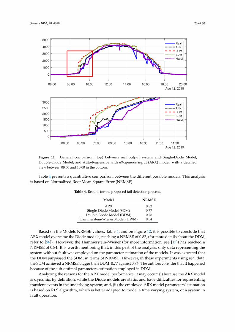
This section presents the results of the fault detection process based on photovoltaic models andadaptive thresholds. Figure 11 shows, graphically, the performance of Single-Diode Model (SDM),Double-Diode Model (DDM), ARX model, and Hammerstein–Wiener Model (HWM) as compared tothe real output system.

Sensors 2020, 20, 4688 20 of 30

11:10 11:20 11:30

May 01, 2020

800

1000

1200

1400

1600

1800

2000

2200

2400

DC

pow

er

(watts)

Real

Simulated

11:10 11:11 11:12 11:13 11:14 11:15 11:16 11:17 11:18

May 01, 2020

1600

1700

1800

1900

2000

2100

2200

2300

2400

DC

pow

er

(watts)

Real

Simulated

Figure 11: 2 Figures side by side

06:00 08:00 10:00 12:00 14:00 16:00 18:00 20:00

Aug 12, 2019

0

1000

2000

3000

4000

5000Real

ARX

DDM

SDM

HWM

08:00 08:30 09:00 09:30 10:00 10:30 11:00 11:30

Aug 12, 2019

0

500

1000

1500

2000

2500

3000Real

ARX

DDM

SDM

HWM


7

Figure 11. General comparison (top) between real output system and Single-Diode Model,Double-Diode Model, and Auto-Regressive with eXogenous input (ARX) model, with a detailedview between 08:30 and 10:00 in the bottom.

Table 4 presents a quantitative comparison, between the different possible models. This analysisis based on Normalized Root Mean Square Error (NRMSE).

Table 4. Results for the proposed fail detection process.

Model NRMSE

ARX 0.82Single-Diode Model (SDM) 0.77

Double-Diode Model (DDM) 0.76Hammerstein-Wiener Model (HWM) 0.84

Based on the Models NRMSE values, Table 4, and on Figure 12, it is possible to conclude thatARX model overcame the Diode models, reaching a NRMSE of 0.82, (for more details about the DDM,refer to [56]). However, the Hammerstein–Wiener (for more information, see [17]) has reached aNRMSE of 0.84. It is worth mentioning that, in this part of the analysis, only data representing thesystem without fault was employed on the parameter estimation of the models. It was expected thatthe DDM surpassed the SDM, in terms of NRMSE. However, in these experiments using real data,the SDM achieved a NRMSE bigger than DDM, 0.77 against 0.76. The authors consider that it happenedbecause of the sub-optimal parameters estimation employed in DDM.

Analyzing the reasons for the ARX model performance, it may occur: (i) because the ARX modelis dynamic, by definition, while the Diode models are static, and have difficulties for representingtransient events in the underlying system; and, (ii) the employed ARX model parameters’ estimationis based on RLS algorithm, which is better adapted to model a time varying system, or a system infault operation.

Sensors 2020, 20, 4688 21 of 30

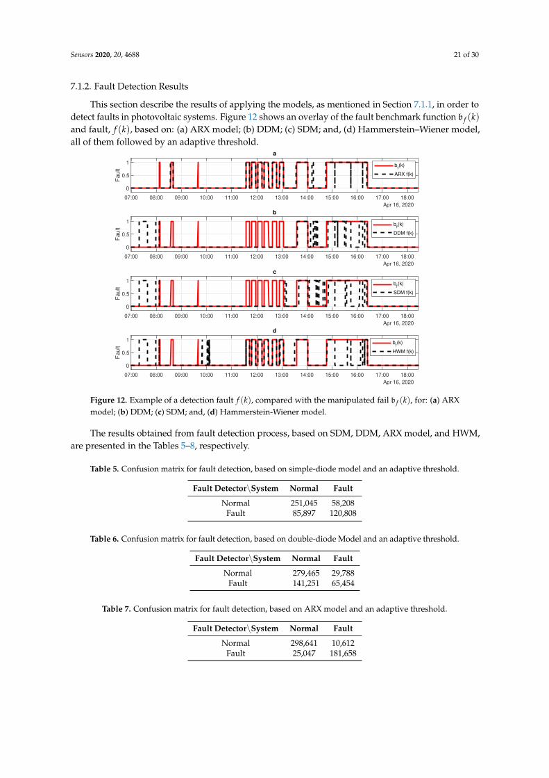
7.1.2. Fault Detection Results

This section describe the results of applying the models, as mentioned in Section 7.1.1, in order todetect faults in photovoltaic systems. Figure 12 shows an overlay of the fault benchmark function b f (k)and fault, f (k), based on: (a) ARX model; (b) DDM; (c) SDM; and, (d) Hammerstein–Wiener model,all of them followed by an adaptive threshold.

1 1.2 1.4 1.6 1.8

105

1.7

1.8

1.9

2

2.1

2.2

a1(k)

1 1.2 1.4 1.6 1.8

105

-1.2

-1

-0.8

-0.6

-0.4

-0.2

a2(k)

1 1.2 1.4 1.6 1.8

105

-6

-4

-2

0

2

b0(k)

1 1.2 1.4 1.6 1.8

105

-2

0

2

4

6

b1(k)


07:00 08:00 09:00 10:00 11:00 12:00 13:00 14:00 15:00 16:00 17:00 18:00

Apr 16, 2020

0

0.5

1

Fa

ult

a

bf(k)

ARX f(k)

07:00 08:00 09:00 10:00 11:00 12:00 13:00 14:00 15:00 16:00 17:00 18:00

Apr 16, 2020

0

0.5

1

Fa

ult

b

bf(k)

DDM f(k)

07:00 08:00 09:00 10:00 11:00 12:00 13:00 14:00 15:00 16:00 17:00 18:00

Apr 16, 2020

0

0.5

1

Fa

ult

c

bf(k)

SDM f(k)

07:00 08:00 09:00 10:00 11:00 12:00 13:00 14:00 15:00 16:00 17:00 18:00

Apr 16, 2020

0

0.5

1

Fa

ult

d

bf(k)

HWM f(k)


8

Figure 12. Example of a detection fault f (k), compared with the manipulated fail b f (k), for: (a) ARXmodel; (b) DDM; (c) SDM; and, (d) Hammerstein-Wiener model.

The results obtained from fault detection process, based on SDM, DDM, ARX model, and HWM,are presented in the Tables 5–8, respectively.

Table 5. Confusion matrix for fault detection, based on simple-diode model and an adaptive threshold.

Fault Detector\System Normal Fault

Normal 251,045 58,208Fault 85,897 120,808

Table 6. Confusion matrix for fault detection, based on double-diode Model and an adaptive threshold.


Normal 279,465 29,788Fault 141,251 65,454

Table 7. Confusion matrix for fault detection, based on ARX model and an adaptive threshold.


Normal 298,641 10,612Fault 25,047 181,658

Sensors 2020, 20, 4688 22 of 30

Table 8. Confusion matrix for fault detection, based on Hammerstein-Wiener model and anadaptive threshold.


Normal 223,562 85,691Fault 93,634 113,071

Tables 5–8 show the raw data used to calculate the overall efficiency of the proposed fault detectionprocess (Table 9). However, some inferences can be done even using the raw data. Among the testedcases, ARX models (Table 7) present: (i) the best ability to point out correctly when the system isoperating normally (298,641 detections); (ii) the best capacity to discern when the system is operatingin fault (181,658 detections); (iii) the lowest number of false positives (10,612 detections); and, (iv)the lowest number of false negatives (25,047 detections). These characteristics and the performancecomparison among the models can be summarized in the Table 9.

Table 9. Fault detection results for the Diode, ARX, and Hamerstein models in photovoltaic systems.

Property ARX [%] Simple-Diode [%] Double-Diode [%] Hammerstein- Wiener [%]

Accuracy 93.09 72.07 74.81 65.24Precision 87.88 58.44 69.09 54.70

Sensitivity 94.48 67.48 68.34 56.89Specificity 92.26 74.51 79.20 70.48

Based on Table 9, one can conclude that ARX model approach overcomes the three other modelsin all analyzed statistical properties. It is important to point out that the overall accuracy offeredby the ARX model is 19.64% greater than the second best model (DDM). It is also worth to mentionthat the detection fault (based on ARX model) is robust in signalizing that the photovoltaic systemis not in fault state, presenting a specificity of 92.26%. On the other hand, its precision is under 90%,representing the detection system can indicate faults erroneously in 12.22% of cases (considering aprecision of 87.88%).

It is important to mention that the HWM was tested in fault detection, in spite of its time invariantnature, which is not advisable for detecting a fault, and its higher computational cost (if comparedwith the others). The SDM and DDM were tested, because they are benchmarks largely employed inthe literature (as presented in Sections 2.3 and 4.2). Furthermore, all of the mentioned models werecoupled with an adaptive threshold, in order to carry out the fault detection process.

The better performance achieved by the ARX model in fault detection may be due to: (i) it is adynamical model (and have advantages if compared with static diode models); (ii) as ARX modelsare dynamic, they can describe the system behavior in both transient and steady state; and, (iii) ARXmodel parameters estimation is based on RLS algorithm, which is better adapted to model a timevarying system (surpassing time invariant models, as Hammerstein–Wiener, in a fault detection).

7.2. Validation of Simulated Data

In Section 4, we proposed a hybrid approach for generating the training dataset. Some preliminarytests were made in order to guarantee that the simulated systems accurately emulates the real systembehavior. For these tests, all of the collected irradiance (g(k)) and temperature (t(k)) pairs from thereal dataset (Section 4.1) were used to generate simulated outputs.

Table 10 shows the Mean Absolute Percentage Error (MAPE) between real and simulated data fornormal operation and for each of proposed faults except from open-circuit, which outputs zero. It canbe seen from the results that a maximum MAPE of 2.59% is observed for the normal operation, which issufficiently small to not affect classification accuracy, when the system is trained using simulateddata only. In addition, an excerpt of the generated data was plot in Figure 13, which shows a visualconcordance between real and simulated data.

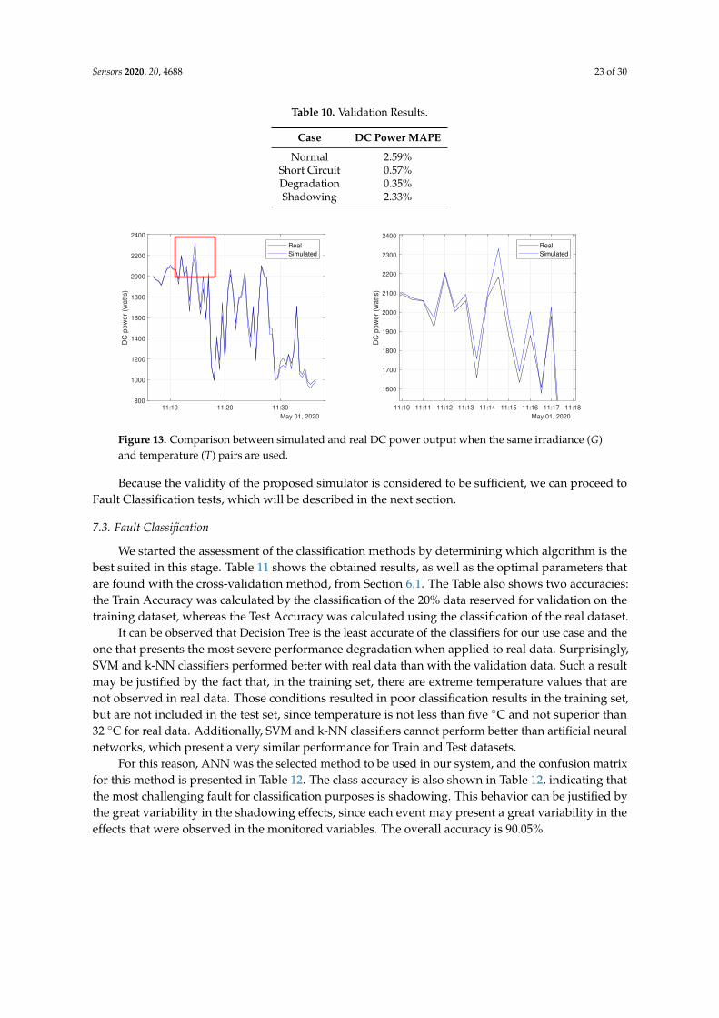
Sensors 2020, 20, 4688 23 of 30

Table 10. Validation Results.

Case DC Power MAPE

Normal 2.59%Short Circuit 0.57%Degradation 0.35%Shadowing 2.33%

11:10 11:20 11:30

May 01, 2020

800

1000

1200

1400

1600

1800

2000

2200

2400

DC

po

we

r (w

att

s)

Real

Simulated

11:10 11:11 11:12 11:13 11:14 11:15 11:16 11:17 11:18

May 01, 2020

1600

1700

1800

1900

2000

2100

2200

2300

2400

DC

po

we

r (w

att

s)

Real

Simulated

Figure 11: 2 Figures side by side

06:00 08:00 10:00 12:00 14:00 16:00 18:00 20:00

Aug 12, 2019

0

1000

2000

3000

4000

5000

DC

po

we

r (w

att

s)

Real

ARX

Double Diode

Single Diode

08:00 08:30 09:00 09:30 10:00 10:30 11:00 11:30 12:00

Aug 12, 2019

0

1000

2000

3000

DC

po

we

r (w

att

s)

Real

ARX

Double Diode

Single Diode


7

Figure 13. Comparison between simulated and real DC power output when the same irradiance (G)and temperature (T) pairs are used.

Because the validity of the proposed simulator is considered to be sufficient, we can proceed toFault Classification tests, which will be described in the next section.

7.3. Fault Classification

We started the assessment of the classification methods by determining which algorithm is thebest suited in this stage. Table 11 shows the obtained results, as well as the optimal parameters thatare found with the cross-validation method, from Section 6.1. The Table also shows two accuracies:the Train Accuracy was calculated by the classification of the 20% data reserved for validation on thetraining dataset, whereas the Test Accuracy was calculated using the classification of the real dataset.

It can be observed that Decision Tree is the least accurate of the classifiers for our use case and theone that presents the most severe performance degradation when applied to real data. Surprisingly,SVM and k-NN classifiers performed better with real data than with the validation data. Such a resultmay be justified by the fact that, in the training set, there are extreme temperature values that arenot observed in real data. Those conditions resulted in poor classification results in the training set,but are not included in the test set, since temperature is not less than five ◦C and not superior than32 ◦C for real data. Additionally, SVM and k-NN classifiers cannot perform better than artificial neuralnetworks, which present a very similar performance for Train and Test datasets.

For this reason, ANN was the selected method to be used in our system, and the confusion matrixfor this method is presented in Table 12. The class accuracy is also shown in Table 12, indicating thatthe most challenging fault for classification purposes is shadowing. This behavior can be justified bythe great variability in the shadowing effects, since each event may present a great variability in theeffects that were observed in the monitored variables. The overall accuracy is 90.05%.

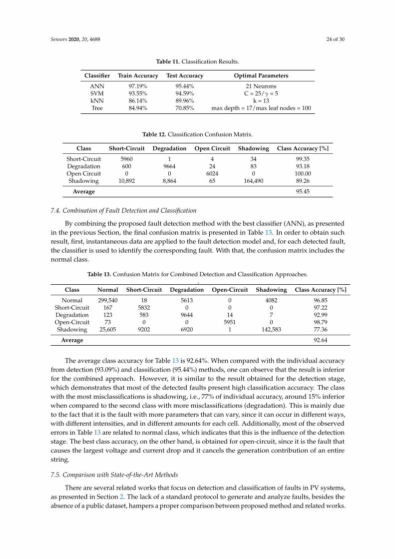
Sensors 2020, 20, 4688 24 of 30

Table 11. Classification Results.

Classifier Train Accuracy Test Accuracy Optimal Parameters

ANN 97.19% 95.44% 21 NeuronsSVM 93.55% 94.59% C = 25/γ = 5kNN 86.14% 89.96% k = 13Tree 84.94% 70.85% max depth = 17/max leaf nodes = 100

Table 12. Classification Confusion Matrix.

Class Short-Circuit Degradation Open Circuit Shadowing Class Accuracy [%]

Short-Circuit 5960 1 4 34 99.35Degradation 600 9664 24 83 93.18Open Circuit 0 0 6024 0 100.00Shadowing 10,892 8,864 65 164,490 89.26

Average 95.45

7.4. Combination of Fault Detection and Classification

By combining the proposed fault detection method with the best classifier (ANN), as presentedin the previous Section, the final confusion matrix is presented in Table 13. In order to obtain suchresult, first, instantaneous data are applied to the fault detection model and, for each detected fault,the classifier is used to identify the corresponding fault. With that, the confusion matrix includes thenormal class.

Table 13. Confusion Matrix for Combined Detection and Classification Approaches..

Class Normal Short-Circuit Degradation Open-Circuit Shadowing Class Accuracy [%]

Normal 299,540 18 5613 0 4082 96.85Short-Circuit 167 5832 0 0 0 97.22Degradation 123 583 9644 14 7 92.99Open-Circuit 73 0 0 5951 0 98.79Shadowing 25,605 9202 6920 1 142,583 77.36

Average 92.64

The average class accuracy for Table 13 is 92.64%. When compared with the individual accuracyfrom detection (93.09%) and classification (95.44%) methods, one can observe that the result is inferiorfor the combined approach. However, it is similar to the result obtained for the detection stage,which demonstrates that most of the detected faults present high classification accuracy. The classwith the most misclassifications is shadowing, i.e., 77% of individual accuracy, around 15% inferiorwhen compared to the second class with more misclassifications (degradation). This is mainly dueto the fact that it is the fault with more parameters that can vary, since it can occur in different ways,with different intensities, and in different amounts for each cell. Additionally, most of the observederrors in Table 13 are related to normal class, which indicates that this is the influence of the detectionstage. The best class accuracy, on the other hand, is obtained for open-circuit, since it is the fault thatcauses the largest voltage and current drop and it cancels the generation contribution of an entirestring.

7.5. Comparison with State-of-the-Art Methods

There are several related works that focus on detection and classification of faults in PV systems,as presented in Section 2. The lack of a standard protocol to generate and analyze faults, besides theabsence of a public dataset, hampers a proper comparison between proposed method and related works.

Sensors 2020, 20, 4688 25 of 30

However, by selecting works that detect and classify similar faults, we can present a comparison withstate-of-the-art models.

The recent works from [39,40] present a similar two-stage architecture when compared withthis work. Additionally, they use auto regressive models to estimate the expected power output asa function of current environmental conditions. The difference lies in the fault detection methods,which makes the works complimentary. While [39,40] uses fuzzy inference models yielding 98.2%accuracy with 16 combinations of shadowing, short circuit and open circuit, they cannot operatewithout disturbing the normal operation of the system, disconnecting the whole system to evaluateVxI curves or run the tree search algorithm.

The proposal from [42,45], on the other hand, works when the PV modules are normally operating.The first achieved 100% accuracy when detecting short circuit and open circuit faults while the secondyielded overall accuracy of 97.52% for the same faults. This way, we observe a similar performancefor the mentioned faults when compared to our proposed methods, which yields 97.22% accuracy forshort-circuit and 98.78% for open circuit faults.

Moreover, we argue that our work is complementary to the mentioned since our proposed systemis installed in a plant that generates more power (5 kW vs 1.8 kW), is installed in a region withmore panel temperature variation (40 ◦C vs 7 ◦C) and can detect Shadowing and Degradation faultsbesides different short/open circuit conditions. In addition, we can achieve 92.64% of overall accuracy(detection and classification) while presenting some advantages that can be summarized, as follows:

• it allows real-time fault detection and classification (detection and classification are performedevery second), keeping the PV plant in operation (without disconnection);

• shadowing events are caused by real shadowing, which makes it difficult to characterize,unlike the controlled shadowing presented in [11,38] that normally increases the performance forthat class; and,

• it presents a comparable performance to other works, notwithstanding those works use differentdatabases and classification procedures.

7.6. Monitoring System

Finally, this section describes the implemented system that collects all of the data to make themavailable in an execution environment to run the fault detection and fault classification algorithms.The calculated results are indicated as the current status of the PV plant. Figure 14 shows one of theHMI screens, namely the real-time tab, in which all instantaneous and integrated monitored signals,both electrical and environmental, can be viewed together with the system inferred status. The datadisposition follows the generation on the PV strings in the left, the inverter and its parameter inthe center, and the output of two phases at the right. The upper and right hand strips show theenvironmental conditions and performance. In this tab, pre-built and user configurable alarms canalso be set. The HMI also implements a performance evaluation tab and a history tab, in which aconfigurable graph of the chosen signals can be plotted in a chosen time window. Because the systemis a test bench for monitoring strategies, further details are reported in other work [8].

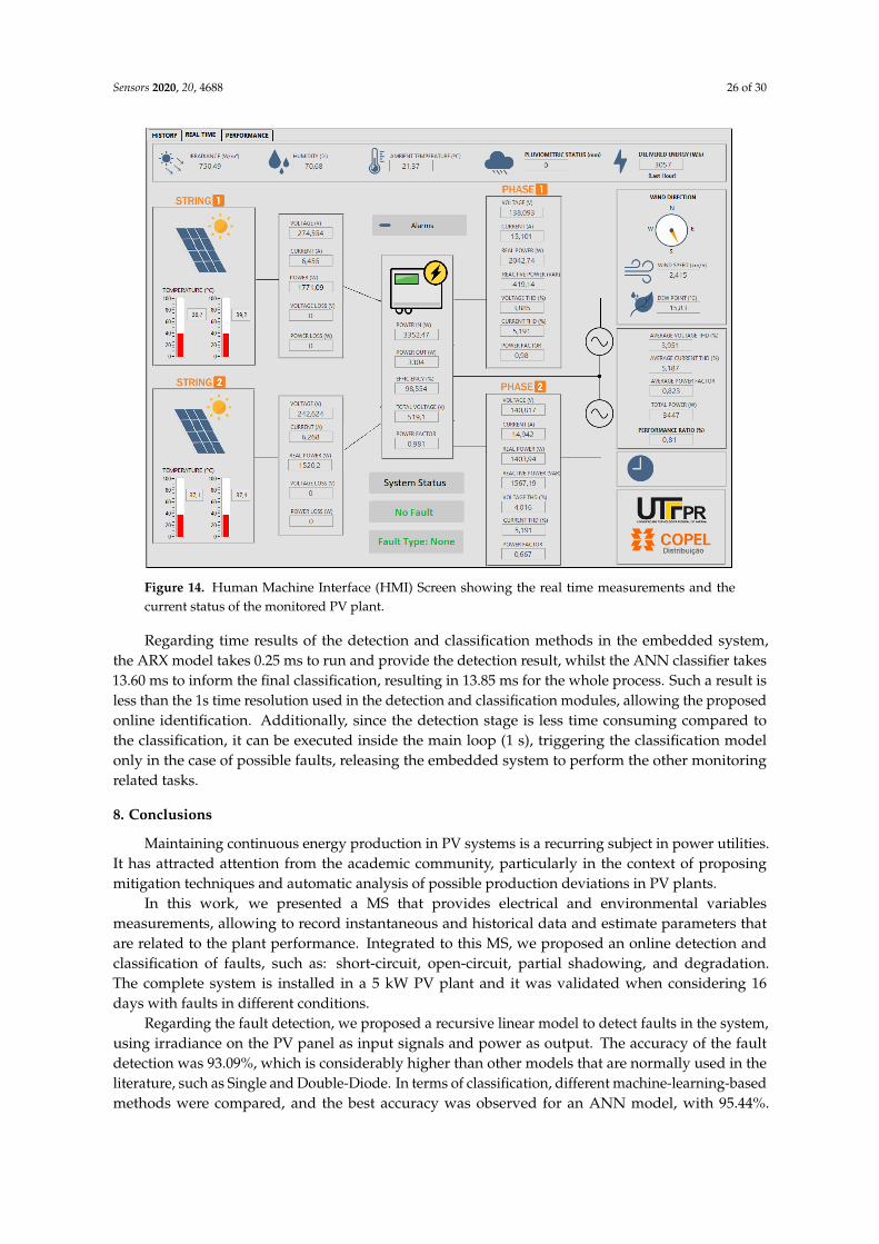
Sensors 2020, 20, 4688 26 of 30

Figure 14. Human Machine Interface (HMI) Screen showing the real time measurements and thecurrent status of the monitored PV plant.

Regarding time results of the detection and classification methods in the embedded system,the ARX model takes 0.25 ms to run and provide the detection result, whilst the ANN classifier takes13.60 ms to inform the final classification, resulting in 13.85 ms for the whole process. Such a result isless than the 1s time resolution used in the detection and classification modules, allowing the proposedonline identification. Additionally, since the detection stage is less time consuming compared tothe classification, it can be executed inside the main loop (1 s), triggering the classification modelonly in the case of possible faults, releasing the embedded system to perform the other monitoringrelated tasks.

8. Conclusions

Maintaining continuous energy production in PV systems is a recurring subject in power utilities.It has attracted attention from the academic community, particularly in the context of proposingmitigation techniques and automatic analysis of possible production deviations in PV plants.

In this work, we presented a MS that provides electrical and environmental variablesmeasurements, allowing to record instantaneous and historical data and estimate parameters thatare related to the plant performance. Integrated to this MS, we proposed an online detection andclassification of faults, such as: short-circuit, open-circuit, partial shadowing, and degradation.The complete system is installed in a 5 kW PV plant and it was validated when considering 16days with faults in different conditions.

Regarding the fault detection, we proposed a recursive linear model to detect faults in the system,using irradiance on the PV panel as input signals and power as output. The accuracy of the faultdetection was 93.09%, which is considerably higher than other models that are normally used in theliterature, such as Single and Double-Diode. In terms of classification, different machine-learning-basedmethods were compared, and the best accuracy was observed for an ANN model, with 95.44%.

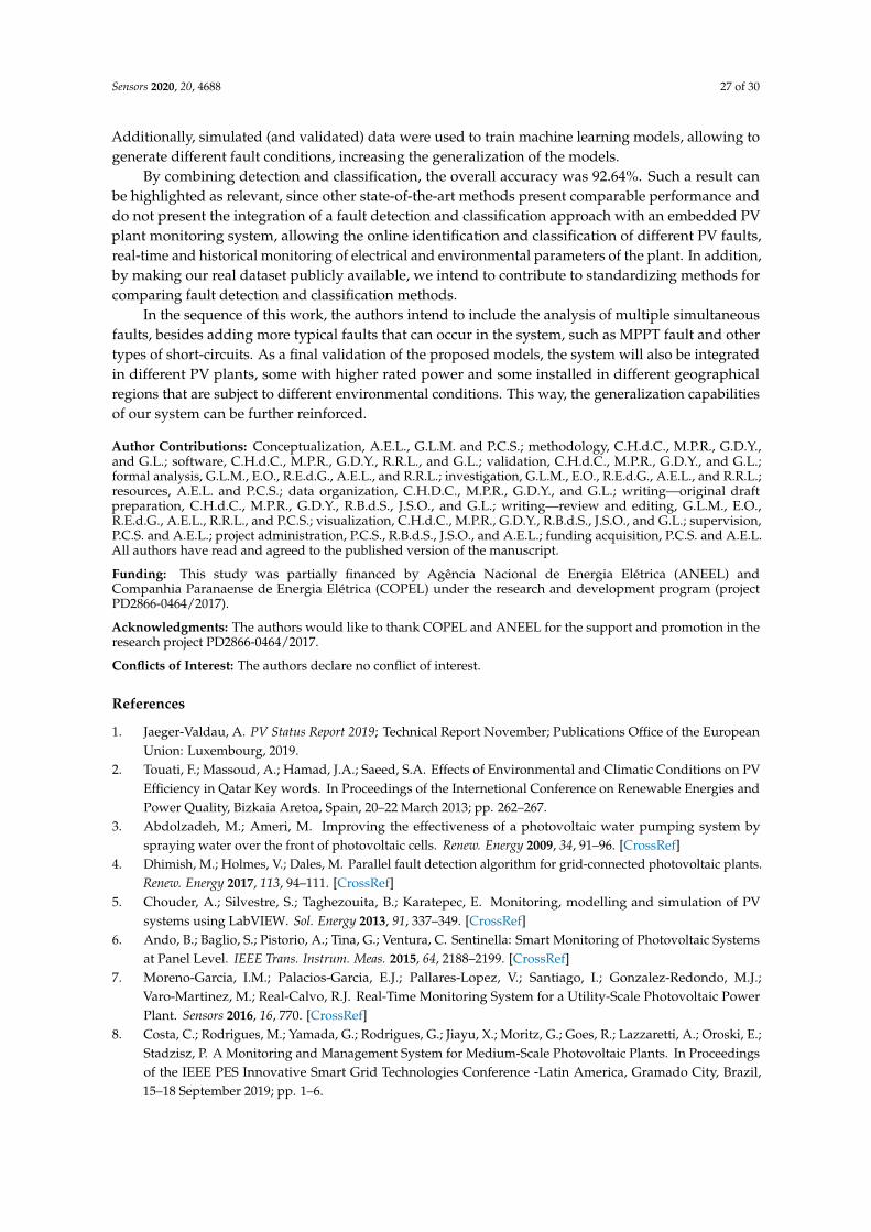
Sensors 2020, 20, 4688 27 of 30

Additionally, simulated (and validated) data were used to train machine learning models, allowing togenerate different fault conditions, increasing the generalization of the models.

By combining detection and classification, the overall accuracy was 92.64%. Such a result canbe highlighted as relevant, since other state-of-the-art methods present comparable performance anddo not present the integration of a fault detection and classification approach with an embedded PVplant monitoring system, allowing the online identification and classification of different PV faults,real-time and historical monitoring of electrical and environmental parameters of the plant. In addition,by making our real dataset publicly available, we intend to contribute to standardizing methods forcomparing fault detection and classification methods.

In the sequence of this work, the authors intend to include the analysis of multiple simultaneousfaults, besides adding more typical faults that can occur in the system, such as MPPT fault and othertypes of short-circuits. As a final validation of the proposed models, the system will also be integratedin different PV plants, some with higher rated power and some installed in different geographicalregions that are subject to different environmental conditions. This way, the generalization capabilitiesof our system can be further reinforced.

Author Contributions: Conceptualization, A.E.L., G.L.M. and P.C.S.; methodology, C.H.d.C., M.P.R., G.D.Y.,and G.L.; software, C.H.d.C., M.P.R., G.D.Y., R.R.L., and G.L.; validation, C.H.d.C., M.P.R., G.D.Y., and G.L.;formal analysis, G.L.M., E.O., R.E.d.G., A.E.L., and R.R.L.; investigation, G.L.M., E.O., R.E.d.G., A.E.L., and R.R.L.;resources, A.E.L. and P.C.S.; data organization, C.H.D.C., M.P.R., G.D.Y., and G.L.; writing—original draftpreparation, C.H.d.C., M.P.R., G.D.Y., R.B.d.S., J.S.O., and G.L.; writing—review and editing, G.L.M., E.O.,R.E.d.G., A.E.L., R.R.L., and P.C.S.; visualization, C.H.d.C., M.P.R., G.D.Y., R.B.d.S., J.S.O., and G.L.; supervision,P.C.S. and A.E.L.; project administration, P.C.S., R.B.d.S., J.S.O., and A.E.L.; funding acquisition, P.C.S. and A.E.L.All authors have read and agreed to the published version of the manuscript.

Funding: This study was partially financed by Agência Nacional de Energia Elétrica (ANEEL) andCompanhia Paranaense de Energia Elétrica (COPEL) under the research and development program (projectPD2866-0464/2017).

Acknowledgments: The authors would like to thank COPEL and ANEEL for the support and promotion in theresearch project PD2866-0464/2017.

Conflicts of Interest: The authors declare no conflict of interest.

References

1. Jaeger-Valdau, A. PV Status Report 2019; Technical Report November; Publications Office of the EuropeanUnion: Luxembourg, 2019.

2. Touati, F.; Massoud, A.; Hamad, J.A.; Saeed, S.A. Effects of Environmental and Climatic Conditions on PVEfficiency in Qatar Key words. In Proceedings of the Internetional Conference on Renewable Energies andPower Quality, Bizkaia Aretoa, Spain, 20–22 March 2013; pp. 262–267.

3. Abdolzadeh, M.; Ameri, M. Improving the effectiveness of a photovoltaic water pumping system byspraying water over the front of photovoltaic cells. Renew. Energy 2009, 34, 91–96. [CrossRef]

4. Dhimish, M.; Holmes, V.; Dales, M. Parallel fault detection algorithm for grid-connected photovoltaic plants.Renew. Energy 2017, 113, 94–111. [CrossRef]

5. Chouder, A.; Silvestre, S.; Taghezouita, B.; Karatepec, E. Monitoring, modelling and simulation of PVsystems using LabVIEW. Sol. Energy 2013, 91, 337–349. [CrossRef]

6. Ando, B.; Baglio, S.; Pistorio, A.; Tina, G.; Ventura, C. Sentinella: Smart Monitoring of Photovoltaic Systemsat Panel Level. IEEE Trans. Instrum. Meas. 2015, 64, 2188–2199. [CrossRef]

7. Moreno-Garcia, I.M.; Palacios-Garcia, E.J.; Pallares-Lopez, V.; Santiago, I.; Gonzalez-Redondo, M.J.;Varo-Martinez, M.; Real-Calvo, R.J. Real-Time Monitoring System for a Utility-Scale Photovoltaic PowerPlant. Sensors 2016, 16, 770. [CrossRef]

8. Costa, C.; Rodrigues, M.; Yamada, G.; Rodrigues, G.; Jiayu, X.; Moritz, G.; Goes, R.; Lazzaretti, A.; Oroski, E.;Stadzisz, P. A Monitoring and Management System for Medium-Scale Photovoltaic Plants. In Proceedingsof the IEEE PES Innovative Smart Grid Technologies Conference -Latin America, Gramado City, Brazil,15–18 September 2019; pp. 1–6.

http://dx.doi.org/10.1016/j.renene.2008.03.024


http://dx.doi.org/10.1016/j.solener.2012.09.016

http://dx.doi.org/10.1109/TIM.2014.2386931

http://dx.doi.org/10.3390/s16060770

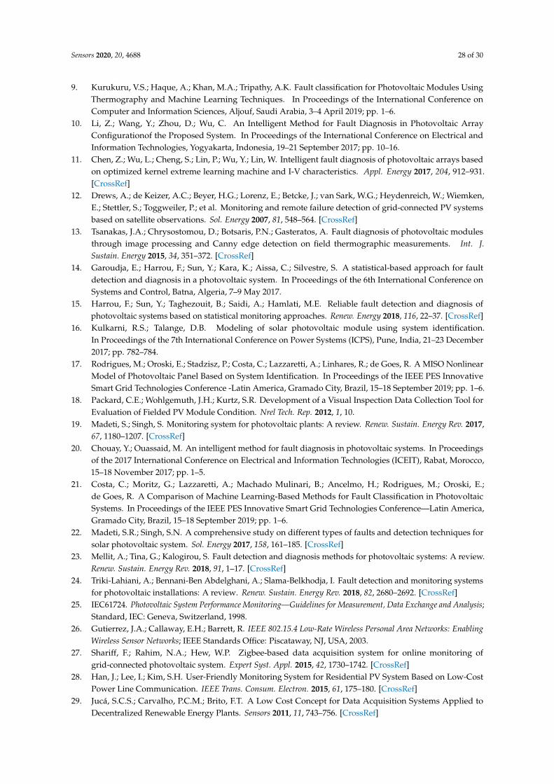
Sensors 2020, 20, 4688 28 of 30

9. Kurukuru, V.S.; Haque, A.; Khan, M.A.; Tripathy, A.K. Fault classification for Photovoltaic Modules UsingThermography and Machine Learning Techniques. In Proceedings of the International Conference onComputer and Information Sciences, Aljouf, Saudi Arabia, 3–4 April 2019; pp. 1–6.

10. Li, Z.; Wang, Y.; Zhou, D.; Wu, C. An Intelligent Method for Fault Diagnosis in Photovoltaic ArrayConfigurationof the Proposed System. In Proceedings of the International Conference on Electrical andInformation Technologies, Yogyakarta, Indonesia, 19–21 September 2017; pp. 10–16.

11. Chen, Z.; Wu, L.; Cheng, S.; Lin, P.; Wu, Y.; Lin, W. Intelligent fault diagnosis of photovoltaic arrays basedon optimized kernel extreme learning machine and I-V characteristics. Appl. Energy 2017, 204, 912–931.[CrossRef]

12. Drews, A.; de Keizer, A.C.; Beyer, H.G.; Lorenz, E.; Betcke, J.; van Sark, W.G.; Heydenreich, W.; Wiemken,E.; Stettler, S.; Toggweiler, P.; et al. Monitoring and remote failure detection of grid-connected PV systemsbased on satellite observations. Sol. Energy 2007, 81, 548–564. [CrossRef]

13. Tsanakas, J.A.; Chrysostomou, D.; Botsaris, P.N.; Gasteratos, A. Fault diagnosis of photovoltaic modulesthrough image processing and Canny edge detection on field thermographic measurements. Int. J.Sustain. Energy 2015, 34, 351–372. [CrossRef]

14. Garoudja, E.; Harrou, F.; Sun, Y.; Kara, K.; Aissa, C.; Silvestre, S. A statistical-based approach for faultdetection and diagnosis in a photovoltaic system. In Proceedings of the 6th International Conference onSystems and Control, Batna, Algeria, 7–9 May 2017.

15. Harrou, F.; Sun, Y.; Taghezouit, B.; Saidi, A.; Hamlati, M.E. Reliable fault detection and diagnosis ofphotovoltaic systems based on statistical monitoring approaches. Renew. Energy 2018, 116, 22–37. [CrossRef]

16. Kulkarni, R.S.; Talange, D.B. Modeling of solar photovoltaic module using system identification.In Proceedings of the 7th International Conference on Power Systems (ICPS), Pune, India, 21–23 December2017; pp. 782–784.

17. Rodrigues, M.; Oroski, E.; Stadzisz, P.; Costa, C.; Lazzaretti, A.; Linhares, R.; de Goes, R. A MISO NonlinearModel of Photovoltaic Panel Based on System Identification. In Proceedings of the IEEE PES InnovativeSmart Grid Technologies Conference -Latin America, Gramado City, Brazil, 15–18 September 2019; pp. 1–6.

18. Packard, C.E.; Wohlgemuth, J.H.; Kurtz, S.R. Development of a Visual Inspection Data Collection Tool forEvaluation of Fielded PV Module Condition. Nrel Tech. Rep. 2012, 1, 10.

19. Madeti, S.; Singh, S. Monitoring system for photovoltaic plants: A review. Renew. Sustain. Energy Rev. 2017,67, 1180–1207. [CrossRef]

20. Chouay, Y.; Ouassaid, M. An intelligent method for fault diagnosis in photovoltaic systems. In Proceedingsof the 2017 International Conference on Electrical and Information Technologies (ICEIT), Rabat, Morocco,15–18 November 2017; pp. 1–5.

21. Costa, C.; Moritz, G.; Lazzaretti, A.; Machado Mulinari, B.; Ancelmo, H.; Rodrigues, M.; Oroski, E.;de Goes, R. A Comparison of Machine Learning-Based Methods for Fault Classification in PhotovoltaicSystems. In Proceedings of the IEEE PES Innovative Smart Grid Technologies Conference—Latin America,Gramado City, Brazil, 15–18 September 2019; pp. 1–6.

22. Madeti, S.R.; Singh, S.N. A comprehensive study on different types of faults and detection techniques forsolar photovoltaic system. Sol. Energy 2017, 158, 161–185. [CrossRef]

23. Mellit, A.; Tina, G.; Kalogirou, S. Fault detection and diagnosis methods for photovoltaic systems: A review.Renew. Sustain. Energy Rev. 2018, 91, 1–17. [CrossRef]

24. Triki-Lahiani, A.; Bennani-Ben Abdelghani, A.; Slama-Belkhodja, I. Fault detection and monitoring systemsfor photovoltaic installations: A review. Renew. Sustain. Energy Rev. 2018, 82, 2680–2692. [CrossRef]

25. IEC61724. Photovoltaic System Performance Monitoring—Guidelines for Measurement, Data Exchange and Analysis;Standard, IEC: Geneva, Switzerland, 1998.

26. Gutierrez, J.A.; Callaway, E.H.; Barrett, R. IEEE 802.15.4 Low-Rate Wireless Personal Area Networks: EnablingWireless Sensor Networks; IEEE Standards Office: Piscataway, NJ, USA, 2003.

27. Shariff, F.; Rahim, N.A.; Hew, W.P. Zigbee-based data acquisition system for online monitoring ofgrid-connected photovoltaic system. Expert Syst. Appl. 2015, 42, 1730–1742. [CrossRef]

28. Han, J.; Lee, I.; Kim, S.H. User-Friendly Monitoring System for Residential PV System Based on Low-CostPower Line Communication. IEEE Trans. Consum. Electron. 2015, 61, 175–180. [CrossRef]

29. Jucá, S.C.S.; Carvalho, P.C.M.; Brito, F.T. A Low Cost Concept for Data Acquisition Systems Applied toDecentralized Renewable Energy Plants. Sensors 2011, 11, 743–756. [CrossRef]

http://dx.doi.org/10.1016/j.apenergy.2017.05.034


http://dx.doi.org/10.1080/14786451.2013.826223


http://dx.doi.org/10.1016/j.rser.2016.09.088




http://dx.doi.org/10.1016/j.eswa.2014.10.007

http://dx.doi.org/10.1109/TCE.2015.7150571

http://dx.doi.org/10.3390/s110100743

Sensors 2020, 20, 4688 29 of 30

30. Eke, R.; Kavasoglu, A.S.; Kavasoglu, N. Design and implementation of a low-cost multi-channel temperaturemeasurement system for photovoltaic modules. Measurement 2012, 45, 1499–1509. [CrossRef]

31. Sanchez-Pacheco, F.J.; Sotorrio-Ruiz, P.J.; Heredia-Larrubia, J.R.; Pérez-Hidalgo, F.; de Cardona, M.S.PLC-Based PV Plants Smart Monitoring System: Field Measurements and Uncertainty Estimation.IEEE Trans. Instrum. Meas. 2014, 63, 2215–2222. [CrossRef]

32. Ranhotigamage, C.; Mukhopadhyay, S. Field Trials and Performance Monitoring of Distributed Solar PanelsUsing a Low-Cost Wireless Sensors Network for Domestic Applications. IEEE Sens. J. 2011, 11, 2583–2590.[CrossRef]

33. Xiao, W.; Dunford, W.G.; Capel, A. A novel modeling method for photovoltaic cells. In Proceedings of thePower Electronics Specialists Conference, Aachen, Germany, 20–25 June 2004; Volume 3; pp. 1950–1956.

34. De Soto, W.; Klein, S.; Beckman, W. Improvement and validation of a model for photovoltaic arrayperformance. Sol. Energy 2006, 80, 78–88. [CrossRef]

35. Cojocariu, B.; Petrescu, C.; Stefanoiu, D. Photovoltaic Generators–Modeling and Control. In Proceedingsof the 20th International Conference on Control Systems and Computer Science, Bucharest, Romania,27–29 May 2015; pp. 32–37.

36. Alqahtani, A.; Marafi, S.; Musallam, B.; El Khalek, N.E.D.A. Photovoltaic power forecasting model based onnonlinear system identification. Can. J. Electr. Comput. Eng. 2016, 39, 243–250. [CrossRef]

37. Li, Y.; Su, Y.; Shu, L. An ARMAX model for forecasting the power output of a grid connected photovoltaicsystem. Renew. Energy 2014, 66, 78–89. [CrossRef]

38. Chine, W.; Mellit, A.; Lughi, V.; Malek, A.; Sulligoi, G.; Massi Pavan, A. A novel fault diagnosis techniquefor photovoltaic systems based on artificial neural networks. Renew. Energy 2016, 90, 501–512. [CrossRef]

39. Samara, S.; Natsheh, E. Intelligent PV Panels Fault Diagnosis Method Based on NARX Network andLinguistic Fuzzy Rule-Based Systems. Sustainability 2020, 12, 2011. [CrossRef]

40. Natsheh, E.; Samara, S. Tree Search Fuzzy NARX Neural Network Fault Detection Technique for PV Systemswith IoT Support. Electronics 2020, 9, 1087. [CrossRef]

41. Garoudja, Elyes, E.A. An enhanced machine learning based approach for failures detection and diagnosis ofPV systems. Energy Convers. Manag. 2017, 151, 496–513. [CrossRef]

42. Basnet, B.; Chun, H.; Bang, J. An Intelligent Fault Detection Model for Fault Detection in PhotovoltaicSystems. J. Sens. 2020, 2020, 6960328. [CrossRef]

43. Yi, Z.; Etemadi, A.H. Line-to-line fault detection for photovoltaic arrays based on multi-resolution signaldecomposition and two-stage support vector machine. IEEE Trans. Ind. Electron. 2017, 64, 8546–8556.[CrossRef]

44. Hussain, M.; Dhimish, M.; Titarenko, S.; Mather, P. Artificial neural network based photovoltaic faultdetection algorithm integrating two bi-directional input parameters. Renew. Energy 2020, 155, 1272–1292.[CrossRef]

45. Kurukuru, V.S.B.; Blaabjerg, F.; Khan, M.; Haque, A. A Novel Fault Classification Approach for PhotovoltaicSystems. Energies 2020, 13, 308. [CrossRef]

46. IEEE1459-2010. Standard Definitions for the Measurement of Electric Power Quantities Under Sinusoidal,Nonsinusoidal, Balanced, or Unbalanced Conditions; Standard, IEEE—Institute of Electrical and ElectronicEngineers: Piscataway, NJ, USA, 2010.

47. Nguyen, L.; Low, K.S. A Global Maximum Power Point Tracking Scheme Employing DIRECT SearchAlgorithm for Photovoltaic Systems. Ind. Electron. IEEE Trans. 2010, 57, 3456–3467. [CrossRef]

48. Isermann, R.; Münchhof, M. Identification of Dynamic Systems: An Introduction with Applications, 1st ed.;Advanced Textbooks in Control and Signal Processing; Springer: Berlin/Heidelberg, Germany, 2011;Volume 1.

49. Ljung, L. System Identification: Theory for User, 2nd ed.; Prentice Hall: Upper Saddle River, NJ, USA, 1999.50. Billings, S.A. Nonlinear System Identification: NARMAX Methods in the Time, Frequency, and Spatio-Temporal

Domains, 1st ed.; Wiley: Hoboken, NJ, USA, 2013.51. Isermann, R. Fault-Diagnosis Applications: Model-Based Condition Monitoring: Actuators, Drives, Machinery,

Plants, Sensors, and Fault-tolerant Systems, 1st ed.; Springer: Berlin/Heidelberg, Germany, 2011.52. Young, P.C. Recursive Estimation and Time-Series Analysis: An Introduction for the Student and Practitioner,

2nd ed.; Springer: Berlin/Heidelberg, Germany, 2011.

http://dx.doi.org/10.1016/j.measurement.2012.02.029

http://dx.doi.org/10.1109/TIM.2014.2308972

http://dx.doi.org/10.1109/JSEN.2011.2150214


http://dx.doi.org/10.1109/CJECE.2016.2584081



http://dx.doi.org/10.3390/su12052011

http://dx.doi.org/10.3390/electronics9071087

http://dx.doi.org/10.1016/j.enconman.2017.09.019

http://dx.doi.org/10.1155/2020/6960328

http://dx.doi.org/10.1109/TIE.2017.2703681


http://dx.doi.org/10.3390/en13020308

http://dx.doi.org/10.1109/TIE.2009.2039450

Sensors 2020, 20, 4688 30 of 30

53. Cherkassky, V.S.; Mulier, F. Learning from Data: Concepts, Theory, and Methods, 1st ed.; John Wiley & Sons, Inc.:New York, NY, USA, 1998.

54. Vapnik, V.N. Statistical Learning Theory; Wiley-Interscience: Hoboken, NJ, USA, 1998.55. Kingma, D.P.; Ba, J.L. Adam: A method for stochastic optimization. In Proceedings of the 3rd International

Conference on Learning Representations, ICLR 2015-Conference Track Proceedings, San Diego, CA, USA,7–9 May 2015; pp. 1–15 .

56. Ali, M.H.; Rabhi, A.; El Hajjaji, A.; Tina, G.M. Real time fault detection in photovoltaic systems.Energy Procedia 2017, 111, 914–923. [CrossRef]

© 2020 by the authors. Licensee MDPI, Basel, Switzerland. This article is an open accessarticle distributed under the terms and conditions of the Creative Commons Attribution(CC BY) license (http://creativecommons.org/licenses/by/4.0/).

http://xxx.lanl.gov/abs/1412.6980

http://dx.doi.org/10.1016/j.egypro.2017.03.254

http://creativecommons.org/

http://creativecommons.org/licenses/by/4.0/.

Documents

A Monitoring System for Online Fault Detection and