A Noise Analysis for Recovering Reflectances of the …dlisv03.media.osaka-cu.ac.jp/contents/osakacu/kiyo/111TD...In chapter 5, the overall discussions and conclusions are summarized

A Noise Analysis for Recovering Reflectances of the Objects Being Imaged

September 2012

Mikiya HIRONAGA

A Noise Analysis for Recovering Reflectances of the Objects Being Imaged

画像入力による分光反射率復元に対する

ノイズの影響解析

September 2012

Graduate School of Engineering

Osaka City University

Mikiya HIRONAGA

広永美喜也

i

Preface

Colors of objects vary under various illuminants. Even under the exact same illuminants,

pictures taken by different cameras are not the same because pictures are always under the

influence of the illuminants and the sensitivities of the sensors. Thus, recovering the spectral

reflectances vector r by use of the sensor response vector p is important for a reproduction of

accurate colors or a stable recognition of colored objects, etc. The sensor response p is

determined by p=SLr+e, where S is the matrix representing the spectral sensitivities of the image

sensors, L is the matrix representing the spectral power distributions of the illuminants and e is

the additive noise vector. The recovering reflectances r from the sensor response p is an inverse

problem and largely affected by the noise e. To recover accurate reflectances by applying a

reconstruction matrix W, the study of the noise is required.

Shimano proposed a model estimating the noise variance in an image acquisition device based

on the Wiener estimation. He also derived an evaluation model for the quality of an image

acquisition device. In this thesis, Shimano’s model is examined and extended to an

comprehensive model and a robust frame work is proposed for estimating the noise variance and

analyzing the effect of the noise to the image acquisition.

This thesis is organized as follows;

In chapter 1, the background and the purpose of the study are briefly described.

In chapter 2, the spectral evaluation model for the image acquisition device based on the

Wiener model is examined and the spectral measure of the quality (Qr) of the mage acquisition

device for the recovery of the reflectances is studied and it is shown that the Qr can be applied to

other reconstruction models with experimental results and mathematical proofs.

ii

In chapter 3, it is shown that the above mentioned model stands in the subspace projected by

the sensitivities of the human vision. The colorimetric measure of the quality (Qc) is also applied

to multiple reconstruction models and its noise robustness for the quantization error and

sampling error is examined Also the concept of the NIF (Noise Influence Factor) is proposed and

the reason of the noise sensitivity of an image acquisition device is analyzed.

In chapter 4, the model estimating the noise variance based on the Wiener model is extended

and modified to a comprehensive model with a reconstruction matrix W and it is applied to the

reconstruction matrices of the Wiener and the linear models. The accuracy of the estimation for

the noise variance by the proposed model is confirmed by experiments. The increases in the

mean square errors (MSE) of the reconstruction for the reflectances are examined in the Wiener

and the linear models and it is shown that the effect of the regularization for the increase in the

MSE is well described by the proposed model.

In chapter 5, the overall discussions and conclusions are summarized.

Keywords: spectral reflectances, recovery models, colorimetry, evaluation, spectral

discrimination, noise in imaging systems

iii

Contents

1 Overall Introduction 1

Reference s 6

2 Evaluating a quality of an image acquisition device aimed at the reconstruction of spectral

reflectances by the use of the recovery models 9

2.1 Introduction 10

2.2 Models for the Reconstruction of Spectral Reflectances 12

2.2.1 Wiener Estimation Using Estimated Noise Variance 12

2.2.2 Multiple Regression Analysis 15

2.2.3 Imai-Berns Model 16

2.3 Experimental Procedures 16

2.4 Results and Discussions 19

2.5 Conclusions 22

Reference s 28

3 Noise robustness of a colorimetric evaluation model for image acquisition devices with

different characterization models 33

3.1 Introduction 34

3.2 Models for the Colorimetric Evaluation 37

3.2.1 Wiener Estimation Using Estimated Noise Variance 37

3.2.2 Application of the Multiple Regression Analysis to Fundamental Vector

Evaluation 41

3.2.3 Application of the Imai-Berns Model to Fundamental Vector Evaluation 41



3.4.1 MSE and Qc )( 2σ 45

3.4.2 Effect of the Noise to the Relation between MSE and Qc )( 2σ 46

3.4.3 Effect of the Sampling Bits to MSE 49

3.4.4 Effect of the Sampling Bits to NIF 51

iv

3.4.5 Reason of the Noise Sensitivity 52

3.4.6 Error and Quality Estimation Model 54

3.5 Conclusions 54

Reference s 55

4 Influence of the noise present in an image acquisition system on the accuracy of recovered

spectral reflectances 59

4.1 Introduction 60

4.2 Models 61

4.2.1 Previous Models to Separate the MSE based on the Wiener Estimation 61

4.2.2 Multiple Regression Analysis 63

4.2.3 Imai-Berns Model 63

4.2.4 Linear Model 64

4.3 Proposed Model 65



4.6 Conclusions 78

Reference s 79

5 Overall Conclusions 83

v

List of Figures

1.1 Concepts of spectral and colorimetric; vectors projected onto human visual subspace (HVSS).

2.1 Spectral sensitivities of the sensors of the camera.

2.2 Spectral power distribution of the illumination.

2.3 MSEs of the recovered spectral reflectances by the Wiener, Regression, and Imai-Berns

method for the GretagMacbeth ColorChecker (CC) and the Kodak Q60R1 (KK) are plotted

as a function of Qr )( 2σ .

2.4 MSEs of the recovered spectral reflectances by the Wiener, Regression, and Imai-Berns

method for the GretagMacbeth ColorChecker (CC) and the Kodak Q60R1 (KK) are plotted

as a function of Qr )0( , which is the value of Qr )( 2σ when the estimated noise variance is

zero. This is the case without consideration for the noise.

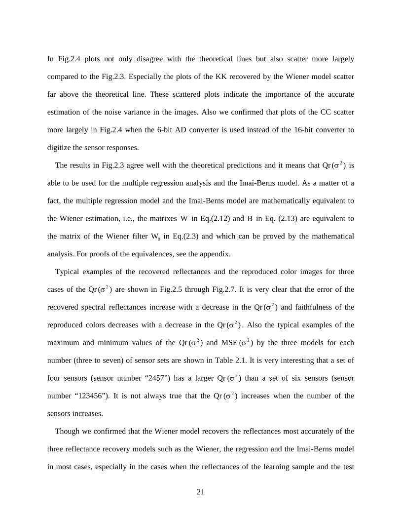
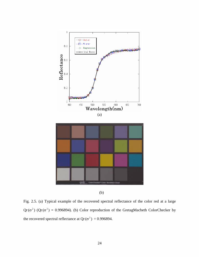
2.5 (a) Typical example of the recovered spectral reflectance of the color red at a large Qr )( 2σ

(Qr )( 2σ = 0.996894). (b) Color reproduction of the GretagMacbeth ColorChecker by the

recovered spectral reflectance at Qr )( 2σ = 0.996894.

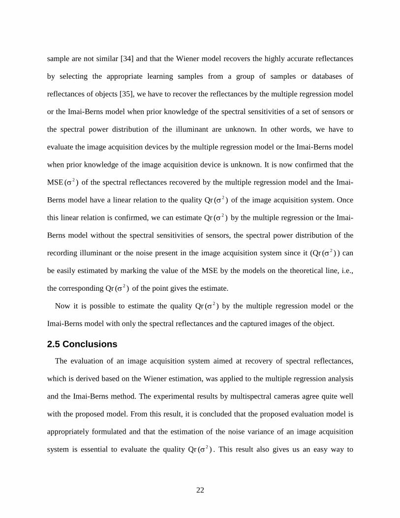
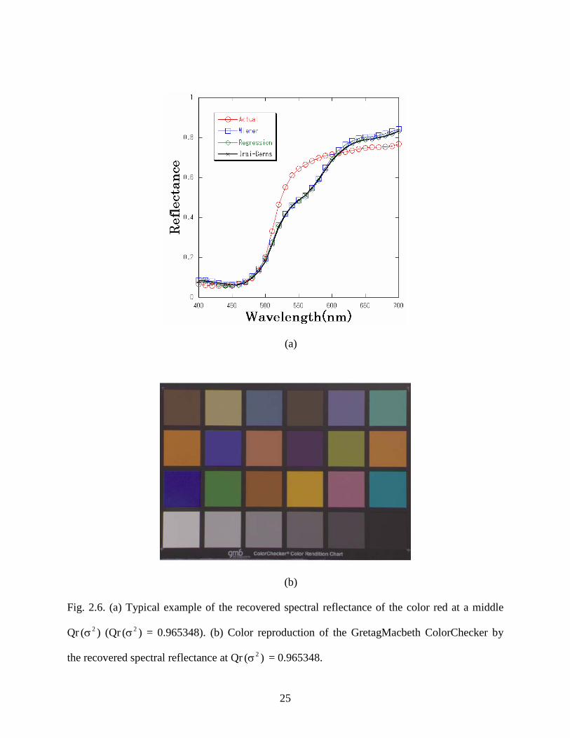
2.6 (a) Typical example of the recovered spectral reflectance of the color red at a middle Qr )( 2σ



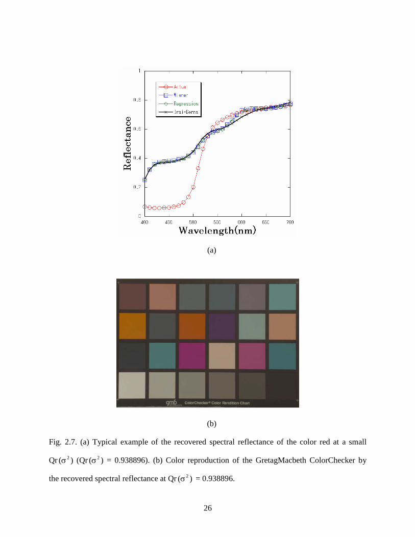
2.7 (a) Typical example of the recovered spectral reflectance of the color red at a small Qr )( 2σ



3.1 Spectral sensitivities of the sensors of the camera sampled at 1nm.

3.2 Spectral power distribution of the illumination sampled at 1nm.

vi

3.3 MSEs of the recovered fundamental vectors by the Wiener, Regression, and Imai-Berns model

for the GretagMacbeth ColorChecker (CC) and the Kodak Q60R1 (KK) are plotted as a

function of Qc )( 2σ .


for GretagMacbeth ColorChecker (CC) are plotted as a function of Qc )( 2σ with (a)8-bit

image and 10-nm sampling intervals, (b)8-bit image and 20-nm sampling intervals, (c)6-bit

image and 10-nm sampling intervals, and (d)6-bit image and 20-nm sampling intervals


for GretagMacbeth ColorChecker (CC) are plotted as a function of Qc )0( with 6-bit image

and 10-nm sampling intervals (MSE )0( s are plotted for the Wiener model).


for GretagMacbeth ColorChecker (CC) and the theoretical MSE estimated with Emax(1-

Qc )( 2σ ) with 10-nm sampling intervals are plotted as a function of the sampling bits.

3.7 10nm NIF(Noise Influence Factor) for three sensor sets are plotted as a function of the

sampling bits.

3.8 Noise variance and the square of singular values for the sensor set “1234” and “247” with 8-bit

and 6-bit images, 10-nm sampling intervals.

4.1 Spectral sensitivities of each sensor.

4.2 Spectral power distribution of the recording illumination.

4.3 Relation between the increase in the MSE by the noise estimated by the previous model

( WienerMSE∆ ) and the MSEnoise by the Wiener, Regression, Imai-Berns and linear model for

the GretagMacbeth ColorChecker .

vii

4.4 (a) Relation between the increase in the MSE ( MSE∆ ) by the linear model and the MSENOISE

( ∑=κσ

R

1i2

i2ˆ ) with the noise variance estimated with the previous model for the

GretagMacbeth ColorChecker .

4.4 (b) Relation between the increase in the MSE ( MSE∆ ) by the linear model and the MSENOISE

( ∑=κσ

R

1i2

i2Wˆ ) with the noise variance estimated with the reconstruction matrix W for the


4.5 Relation between the increase in the MSE ( MSE∆ ) and MSENOISE by the Wiener and the

linear model.

4.6 Relation between the increase in the MSE ( MSE∆ ) and the Noise Sensitivity for the

reconstruction matrix W (∑=κ

R

1i2

i ) or the estimated noise variance.

4.7 Relation between the increase in the MSE ( pMSE∆ ) by the Wiener, regression, Imai-Berns

and linear model and the MSENOISE ( ∑=κσ

R

1i2

i2Wˆ ) with the noise variance estimated with the

reconstruction matrix W for the GretagMacbeth ColorChecker .

viii

List of Tables

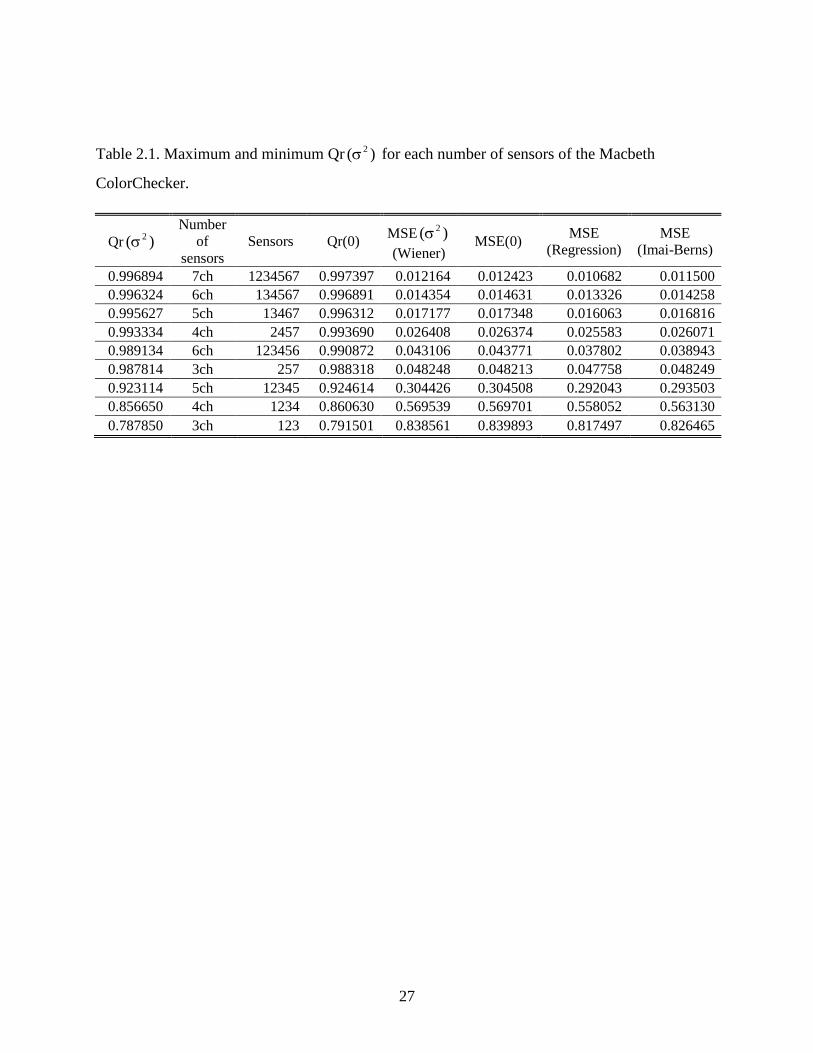
2.1 Maximum and minimum Qr )( 2σ for each number of sensors of the Macbeth ColorChecker.

4.1 Estimated system noise variance and the MSE by the Wiener model with each estimated

system noise variance.

1

Chapter 1

Overall Introduction

This thesis presents a framework for recovering the spectral reflectances of objects being

imaged by an image acquisition system. The proposed work estimates and analyzes the

noise in the image acquisition device and recovers the reflectances of objects accurately.

This chapter addresses the overall introduction of this thesis. The purpose, the background

and the sketch of this thesis are also described in this chapter.

2

The visual information plays an important role for a human being to recognize environments.

The visual information mainly consists of shapes and colors. Colors of objects are dependent on

the illuminant, the surface of the object, and the sensitivity of the sensors. The illuminant and the

sensitivity of the human visual system may vary by circumstances but the spectral reflectances of

objects represent the physical properties of objects. Therefore the recovery of spectral

reflectances of objects is important not only to reproduce color images under various illuminants

[1-3] but also to study computational color vision [4-6] and color constancy [7-9].

Several models have been proposed to recover the spectral reflectances vector r by use of the

sensor response vector p by applying a reconstruction matrix. There are mainly two types of

these models, the first is the Wiener estimation, which minimizes the mean square errors (MSEs)

between the recovered and the measured spectral reflectances [10-12], and the second is the

finite-dimensional linear models of spectral reflectances [13-16]. The spectral sensitivities of the

image sensors S, the spectral power distributions of the illuminants L and the learning samples of

the spectral reflectances vector r which are similar to those of the imaged objects are required for

recovering the spectral reflectances by these two models because a sensor response p is

determined by p=SLr+e, where e is an additive noise vector. Since it is difficult to measure these

spectral characteristics, modifications of these models have been proposed that do not use prior

knowledge of the spectral sensitivities of a set of sensors and the spectral power distribution of

the illuminant. The modification of the Wiener estimation uses the regression analysis [17]

between the known spectral reflectances and the corresponding sensor responses [3,18-22], and

this model is called the pseudoinverse transformation or the regression model [18,23]. Another

modified linear model also uses the regression analysis between the weight column vectors for

the orthonormal basis vectors to represent known spectral reflectances and the corresponding

sensor responses [20,24]; in this model the basis vectors are usually derived by the principal

3

component analysis of spectral the reflectances or derived by singular values decomposition

(SVD) [25]. The modified model is called the Imai-Berns model [26,27].

The recovery of the spectral reflectances vector r from the sensor response p is an inverse

problem. Thus, the accuracy of the estimates depends largely on the noise variance used in the

Wiener estimation. Recently Shimano proposed a new model to estimate the noise variance of an

image acquisition system and also showed that the spectral reflectances of objects being imaged

are recovered accurately by using the Wiener estimation through the use of the image data from a

multispectral camera without prior knowledge of the spectral reflectance of the objects and the

noise present in the image acquisition system [28,29]. He also proposed an evaluation model [30]

based on the Wiener estimation to measure the accuracy of the estimation of the reflectances by

the image acquisition device.

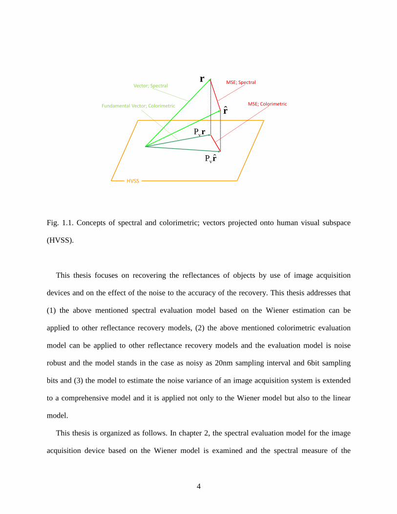
In multispectral color science, there are two methods for computing characteristics of colors.

The one is “spectral” and the other is “colorimetric”. In spectral color processing, every

information of color stimulus obtained from the input device is used, on the other hand in

colorimetric color processing, color stimuli is divided into two parts, the fundamental and the

residual [31]. The fundamental is a projection of a color stimulus onto the human visual subspace

(HVSS) spanned by the sensitivities of the cones of the retina and evokes color sensation to a

human visual system. The residual is an orthogonal part of the color stimulus and evokes no

sensation to a human visual system. The concept for the spectral and the colorimetric is shown in

Fig.1.1. Shimano also showed that his model works well both in spectral and colorimetric cases.

[32,33] .

4

rvP

rPv

r

HVSS

rMSE; Colorimetric

MSE; SpectralVector; Spectral

Fundamental Vector; Colorimetric

Fig. 1.1. Concepts of spectral and colorimetric; vectors projected onto human visual subspace

(HVSS).

This thesis focuses on recovering the reflectances of objects by use of image acquisition

devices and on the effect of the noise to the accuracy of the recovery. This thesis addresses that

(1) the above mentioned spectral evaluation model based on the Wiener estimation can be

applied to other reflectance recovery models, (2) the above mentioned colorimetric evaluation

model can be applied to other reflectance recovery models and the evaluation model is noise

robust and the model stands in the case as noisy as 20nm sampling interval and 6bit sampling

bits and (3) the model to estimate the noise variance of an image acquisition system is extended

to a comprehensive model and it is applied not only to the Wiener model but also to the linear

model.

This thesis is organized as follows. In chapter 2, the spectral evaluation model for the image

acquisition device based on the Wiener model is examined and the spectral measure of the

5

quality (Qr) of the mage acquisition device for the recovery of the reflectances is studied and it is

shown that the Qr can be applied to other reconstruction models with experimental results and

mathematical proofs [34]. In chapter 3, it is shown that the above mentioned model stands in the

subspace projected by the sensitivities of the human vision (HVSS). The colorimetric measure of

the quality (Qc) is also applied to multiple reconstruction models and its noise robustness for the

quantization error and sampling error is examined Also the concept of the NIF (Noise Influence

Factor) is proposed and the reason of the noise sensitivity is analyzed [35]. In chapter 4, the

model estimating the noise variance based on the Wiener model is extended and modified to a

comprehensive model with a reconstruction matrix W and it was applied to the reconstruction

matrices of the Wiener and the linear models. The accuracy of the estimation for the noise

variance by the proposed model is confirmed by experiments. The increases in the mean square

errors (MSE) of the reconstruction for the reflectances are examined in the Wiener and the linear

models and it is shown that the effect of the regularization for the increase in the MSE is well

described by the proposed model. Also the mathematical proof of the equivalence of the

proposed model to the existing model in some conditions is described [36]. In chapter 5, the

overall discussions and conclusions are summarized.

6

References

1. M. D. Fairchild, Color Appearance Models (Addison-Wesley, 1997).

2. Y. Miyake and Y. Yokoyama, “Obtaining and reproduction of accurate color images based

on human perception,” Proc. SPIE 3300, 190.197 (1998).

3. K. Martinez, J. Cupitt, D. Saunders, and R. Pillay, “Ten years of art imaging research,” Proc.

IEEE 90, 28.41 (2002).

4. H. C. Lee, E. J. Breneman, and C. P. Schulte, “Modeling light reflection for computer color

vision,” IEEE Trans. Pattern Anal. Mach. Intell. 12, 79.86 (1990).

5. G. Healey and D. Slater, “Global color constancy: recognition of objects by use of

illumination-invariant properties of color distributions,” J. Opt. Soc. Am. A 11, 3003.3010

(1994).

6. G. J. Klinker, S. A. Shafer, and T. Kanade, “A physical approach to color image

understanding,” Int. J. Comput. Vis. 4, 7.38 (1990).

7. L. T. Maloney and B. A. Wandell, “Color constancy: a method for recovering surface

spectral reflectance,” J. Opt. Soc. Am. A 3, 29.33 (1986).

8. J. Ho, B. V. Funt, and M. S. Drew, “Separating a color signal into illumination and surface

reflectance components: theory and applications,” IEEE Trans. Pattern Anal. Mach. Intell. 12,

966.977 (1990).

9. G. Iverson and M. D’Zumura, “Criteria for color constancy in trichromatic linear models,” J.

Opt. Soc. Am. A 11, 1970.1975 (1994).

10. A. Rosenfeld and A. C. Kak, Digital Picture Processing, 2nd ed. (Academic, 1982).

11. G. Sharma and H. J. Trussell, “Figures of merit for color scanners,” IEEE Trans. Image

Process. 6, 990.1001 (1997).

12. H. Haneishi, T. Hasegawa, N. A. Hosoi, Y. Yokoyama, N. Tsumura, and Y. Miyake,

“System design for accurately estimating the spectral reflectance of art paintings,” Appl. Opt.

39, 6621.6632 (2000).

13. J. Cohen, “Dependency of spectral reflectance curves of the Munsell color chips,” Psychon.

Sci. 1, 369.370 (1964).

7

14. L. T. Maloney, “Evaluation of linear models of surface spectral reflectance with small

numbers of parameters,” J. Opt. Soc. Am. A 3, 1673.1683 (1986).

15. J. P. S. Parkkinen, J. Hallikainen, and T. Jaaskelainen, “Characteristic spectra of Munsell

colors,” J. Opt. Soc. Am. A 6, 318.322 (1989).

16. J. L. Dannemiller, “Spectral reflectance of natural objects: how many basis functions are

necessary?” J. Opt. Soc. Am. A 9, 507.515 (1992).

17. A. A. Afifi and S. P. Azen, Statistical Analysis, (Academic, 1972), Chap. 3.

18. Y. Zhao, L. A. Taplin, M. Nezamabadi, and R. S. Berns, “Using the matrix R method for

spectral image archives,” in Proceedings of The 10th Congress of the International Colour

Association(AIC’5) (International Colour Association, 2005), pp. 469.472.

19. H. L. Shen and H. H. Xin, “Spectral characterization of a color scanner based on optimized

adaptive estimation,” J. Opt. Soc. Am. A 23, 1566.1569 (2006).

20. D. Connah, J. Y. Hardeberg, and S. Westland, “Comparison of linear spectral reconstruction

methods for multispectral imaging,” Proceedings of IEEE’s International Conference on

Image Processing (IEEE, 2004), pp. 1497.1500.

21. Y. Zhao, L. A. Taplin, M. Nezamabadi, and R. S. Berns, “Methods of spectral reflectance

reconstruction for a Sinarback 54 digital camera,” Munsell Color Science Laboratory

Technical Report December 2004, (Munsell Color Science Laboratory, 2004), pp. 1.36.

22. D. Connah and J. Y. Hardeberg, “Spectral recovery using polynomial models,” Proc. SPIE

5667, 65.75 (2005).

23. J. L. Nieves, E. M. Valero, S. M. C. Nascimento, J. H. Andres, and J. Romero, “Multispectral

synthesis of daylight using a commercial digital CCD camera,” Appl. Opt. 44, 5696.5703

(2005).

24. F. H. Imai and R. S. Berns, “Spectral estimation using trichromatic digital cameras,” in

Proceedings of International Symposium on Multispectral Imaging and Color Reproduction

for Digital Archives, (Society of Multispectral Imaging, 1999), pp. 42.49.

25. B. Noble and J. W. Daniel, Applied Linear Algebra, 3rd. ed. (Prentice-Hall, 1988), pp.

338.346.

8

26. M. A. Lopez-Alvarez, J. Hernandez-Andres, Eva. M. Valero, and J. Romero, “Selecting

algorithms, sensors and linear bases for optimum spectral recovery of skylight,” J. Opt. Soc.

Am. A 24, 942.956 (2007).

27. V. Cheung, S. Westland, C. Li, J. Hardeberg, and D. Connah, “Characterization of

trichromatic color cameras by using a new multispectral imaging technique,” J. Opt. Soc. Am.

A 22, 1231.1240 (2005).

28. N. Shimano, “Recovery of spectral reflectances of an art painting without prior knowledge of

objects being imaged,” in Proceedings of The 10th Congress of the International Colour

Association (International Color Association, 2005), pp. 375.378.

29. N. Shimano, “Recovery of spectral reflectances of objects being imaged without prior

knowledge,” IEEE Trans. Image Process. 15, 1848.1856 (2006).

30. N. Shimano, “Evaluation of a multispectral image acquisition system aimed at reconstruction

of spectral reflectances”, Opt. Eng. 44, 107115- 1.107115-6 (2005).

31. J. B. Cohen, “Color and color mixture: scalar and vector fundamentals,”Color Res. Appl. 13,

5.39 (1988).

32. N. Shimano, "Suppression of noise effect in color corrections by spectral sensitivities of

image sensors," Opt. Rev. 9, 81-88(2002).

33. N. Shimano, "Application of a colorimetric evaluation model to multispectral color image

acquisition systems," J. Imaging Sci. Technol. 49, 588-593 (2005).

34. M. Hironaga, N. Shimano, "Evaluating the quality of an image acquisition device aimed at

the reconstruction of spectral reflectances using recovery models," J. Imag. Sci. Technol. 52,

030503(2008).

35. M. Hironaga, N. Shimano, "Noise robustness of a colorimetric evaluation model for image

acquisition devices with different characterization models," Appl. Opt. 48, 5354-5362 (2009).

36. M. Hironaga and N. Shimano, "Estimating the noise variance in an image acquisition system

and its influence on the accuracy of recovered spectral reflectances," Appl. Opt. 49, 6140-

6148 (2010).

9

Chapter 2

Evaluating a quality of an image acquisition device aimed at

the reconstruction of spectral reflectances by the use of the

recovery models

Accurate recovery of spectral reflectances is important for the color reproduction under a

variety of illuminations. To evaluate the quality (Qr) of an image acquisition system aimed

at recovery of spectral reflectances, Shimano proposed an evaluation model based on the

Wiener estimation [Opt. Eng., 44, pp.107115-1-6, 2005.] and showed that mean square

errors (MSE) between the recovered and measured spectral reflectances as a function of Qr

agreed quite well with the prediction by the model.

In this chapter, the evaluation model is applied to two different reflectance recovery

models and it is confirmed that the proposed model can be applied to different models with

experimental results and mathematical proofs.

10

2.1 Introduction

Colors are one of the most important characteristics of the human vision and they have been

heavily studied to acquire accurate information from color images. The acquisition of the

colorimetric information is considered as the acquisition of accurate colorimetric values of

objects through the use of sensor responses [1,2]. The accuracy depends on the spectral

sensitivities of a set of sensors, the noise present in the acquisition device and the spectral

reflectances of the objects etc [1,2]. Therefore the evaluation of the set of sensors is important for

the evaluation of the colorimetric performance or optimization of the spectral sensitivities of the

sensors. Several models have been proposed to evaluate a colorimetric performance of a set of

color sensors [3-7], and the optimization of a set of sensors has been performed based on the

evaluation models [8,9]. However, the application of the evaluation models to real color image

acquisition devices such as digital cameras and color scanners has not appeared because of the

difficulty in estimating noise levels. Recently Shimano proposed a new model to estimate the

noise variance of an image acquisition system [10] and applied it to the proposed colorimetric

evaluation model and a spectral evaluation model, and confirmed that the evaluation model quite

agrees well with the experimental results by multispectral cameras [11].

On the other hand, there is an alternative approach for the color image acquisition. It is the

acquisition of the spectral information of the objects being imaged. The purpose of this approach

is the acquisition of the spectral reflectances of the imaged objects through the use of sensor

responses.[3,12-29]. The acquisition of accurate spectral reflectances of objects is very important

in reproducing a color image under a variety of viewing illuminants [30]. The accuracy of the

recovered spectral reflectances depends on the number of sensors, their spectral sensitivities, the

objects being imaged, the recording illuminants, the noise present in a device and a model used

11

for the recovery. Therefore the evaluation of a camera aimed at the recovery of spectral

reflectances is important for the optimization of an image acquisition system and to get an

intuitive understanding about the acquisition of the spectral information. Shimano already

derived the evaluation model based on the Wiener estimation [31]. The proposed model is

formulated by ( ))(Q1E)(MSE 2rmax

2 σ−=σ , where MSE( 2σ ) is the mean square errors between

the recovered and measured spectral reflectances with the estimated noise variance 2σ , Emax

represents a constant which is determined only by spectral reflectances of objects and Qr )( 2σ is

the quality of the image acquisition system aimed at recovery of spectral reflectances with the

estimated noise variance 2σ . It was shown that Qr )( 2σ is determined by the spectral sensitivities

of the sensors, the spectral power distribution of the recording illuminant, the noise variance of

the image acquisition device and the spectral reflectances of the imaged objects. The model was

applied to the multispectral cameras and it was confirmed that the model agrees quite well with

the experimental results, i.e., the MSE )( 2σ of the recovered spectral reflectances by the Wiener

estimation as a function of the quality Qr )( 2σ of a set of sensors by taking account of the noise

shows the straight line. As Qr )( 2σ is derived from Wiener estimation, it is very important to

confirm whether the model can be applied to other recovery models since the quality Qr )( 2σ is

useful not only for the evaluation of an image acquisition device but also for the optimization of

a set of sensors aimed at recovery of spectral reflectances.

In this chapter, it is shown that Qr )( 2σ has a linear relation to the MSE )( 2σ of the

reflectances recovered by the multiple regression analysis [18] and the Imai-Berns model [26] by

experiments. Mathematical proofs of the equivalence of the Wiener model, the multiple

regression model and the Imai-Berns model are given. It is shown that the Qr )( 2σ is also

appropriately formulated for these models. Once this linear relation is confirmed, we can

estimate Qr )( 2σ by the multiple regression model or the Imai-Berns model, without the spectral

12

sensitivities of the sensors, spectral power distribution of recording illuminant or estimating the

noise variance [32].

This chapter is organized as follows. The outline of the evaluation model and the method to

estimate the noise variance and the models tested are briefly reviewed. In the following sections,

the experimental procedures and the results to demonstrate the trustworthiness of the proposal

are described. The final section presents conclusions and mathematical proofs are in the

appendix section.

2.2 Models for the Reconstruction of Spectral Reflectances

In this section, the derivation of the quality Qr )( 2σ to evaluate the color image acquisition

system and the models used for the experiments are briefly reviewed.

2.2.1 Wiener Estimation Using Estimated Noise Variance

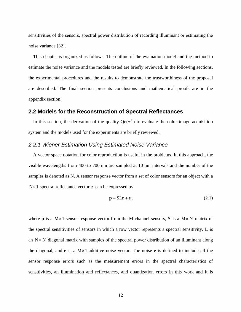
A vector space notation for color reproduction is useful in the problems. In this approach, the

visible wavelengths from 400 to 700 nm are sampled at 10-nm intervals and the number of the

samples is denoted as N. A sensor response vector from a set of color sensors for an object with a

1N× spectral reflectance vector r can be expressed by

erp += SL , (2.1)

where p is a 1M× sensor response vector from the M channel sensors, S is a NM× matrix of

the spectral sensitivities of sensors in which a row vector represents a spectral sensitivity, L is

an NN× diagonal matrix with samples of the spectral power distribution of an illuminant along

the diagonal, and e is a 1M× additive noise vector. The noise e is defined to include all the

sensor response errors such as the measurement errors in the spectral characteristics of

sensitivities, an illumination and reflectances, and quantization errors in this work and it is

13

termed as the system noise[10] below. The system noise is assumed to be signal independent,

zero mean and uncorrelated to itself. For abbreviation, let SLSL = . The mean square errors

(MSE) of the recovered spectral reflectances r is given by

{ }2ÊMSE rr −= , (2.2)

where { }•E represents the expectation. If r is given by pr 0Wˆ = , the matrix 0W which

minimizes the MSE is given by

( ) 12e

TLL

TL0 IRssSSRssSW −

σ+= , (2.3)

where T represents the transpose of a matrix, Rss is an autocorrelation matrix of the spectral

reflectances of samples that will be captured by a device, and 2eσ is the noise variance used for

the estimation. Substitution of Eq.(2.3) into Eq.(2.2) leads to [10]

( )

2iji2

2e

2vj

22vj

4e

1j

N

1i

2iji

1j

N

1ii

N

1i

2e bb)(MSE λ

σ+κ

σκ+σ∑∑+λ∑∑−λ∑=σβ

==

β

===, (2.4)

where iλ is the eigenvalues of Rss , ijb , vjκ and β represent i-th row of the j-th right singular

vector, singular value and a rank of a matrix 2/1LVS Λ , respectively, 2σ is the actual system noise

variance, V is a basis matrix and Λ is an NN× diagonal matrix with positive eigenvalues iλ

along the diagonal in decreasing order. It is easily seen that the MSE is minimized when 22e σ=σ ,

and the MSE )( 2σ is given by

2iji22v

j

2

1j

N

1i

2iji

1j

N

1ii

N

1i

2 bb)(MSE λσ+κ

σ∑∑+λ∑∑−λ∑=σβ

==

β

===. (2.5)

14

Equation (2.5) can be rewritten as

λΣ

λσ+κ

σΣΣ−λΣΣ

−λ∑=σ=

β==

β==

= iN

1i

2iji22v

j

2

1jN

1i2iji1j

N1i

i

N

1i

2

bb

1)MSE( . (2.6)

Therefore the quality of a set of color sensors in the presence of noise is formulated as

i

N1i

2iji22v

j

2

1jN

1i2iji1j

N1i

2r

bb

)(QλΣ

λσ+κ

σΣΣ−λΣΣ

=σ=

β==

β==

. (2.7)

Hence, the MSE )( 2σ is expressed as

( ))(Q1E)MSE( 2rmax

2 σ−=σ , (2.8)

where iN

1imaxE λ∑= = . This equation shows that the MSE )( 2σ has a linear relation to Qr )( 2σ and

the slope of the line is iN

1i λ∑ = . The values of iN

1i λ∑ = are dependent only on the surface spectral

reflectance of the objects being captured. The MSE )( 2σ decreases as the Qr )( 2σ increases to

one.

If we let the noise variance 02e =σ for the Wiener filter in Eq. (2.3), then the MSE )0( is derived

as (by letting 02e =σ in Eq. (2.4))

( ) 2iji2v

j

2

1j

N

1i

2iji

1j

N

1ii

N

1ibb0MSE λ

κ

σ∑∑+λ∑∑−λ∑=β

==

β

===

. (2.9)

The first and second terms on the right-hand side of Eq. (2.9) represent the MSE )0( at a

noiseless case. We denote this MSE as MSEfree, then the estimated system noise variance 2σ can

be represented by

15

( )

2vj

2iji

1jN

1i

free2

bMSE0MSEˆ

κ

λΣΣ

−=σ

β==

, (2.10)

where MSEfree is given by

2iji

1j

N

1ii

N

1ifree bMSE λ∑∑−λ∑=

β

===. (2.11)

Therefore, the system noise variance 2σ can be estimated using Eq. (2.10), since the MSEfree and

the denominator of Eq. (2.10) can be computed if the surface reflectance spectra of objects, the

spectral sensitivities of sensors and the spectral power distribution of an illuminant are known.

The MSE )0( can also be obtained by the experiment using Eqs. (2.2) and (2.3) applying the

Wiener filter with 02e =σ to sensor responses. Therefore, Eq. (2.10) gives a method to estimate

the actual noise variance 2σ . [10]

The quality Qr )( 2σ and MSE )( 2σ can be computed by substituting the estimated noise

variance in Eq.(2.7) and Eq.(2.3) , respectively.

2.2.2 Multiple Regression Analysis

Let ip be a 1M× sensor response vector which is obtained by the image acquisition of a

known spectral reflectance ir of the i-th object, where i represents a number. Let P be a kM×

matrix which contains the sensor responses k21 ,,, ppp , and let R be a kN× matrix which

contains the corresponding spectral reflectances k21 ,,, rrr , where k is the number of the

learning samples. The pseudoinverse model is to find a matrix W which minimizes WPR − ,

where notation • represents the Frobenius norm[33]. The matrix W is given by.

+= RPW , (2.12)

16

where +P represents the pseudo inverse matrix of the matrix P. By applying a matrix W to a

sensor response vector p , i.e., pr Wˆ = , a spectral reflectance is estimated. Therefore this model

does not use the spectral sensitivities of sensors or the spectral power distribution of an

illumination, but it uses only the spectral reflectances of the learning samples.

2.2.3 Imai-Berns Model

The Imai-Berns model [26] is considered as the modification of the linear model by using the

multiple regression analysis between the weight column vectors for basis vectors to represent the

known spectral reflectances and corresponding sensor response vectors.

Let Σ be a kd× matrix which contains the column vectors of the weights k21 ,,, σσσ to

represent the k known spectral reflectances k21 ,,, rrr and let P be a kM× matrix which

contains corresponding sensor response vectors of those reflectances k21 ,,, ppp ,where d is a

number of the weights to represent the spectral reflectances. The multiple regression analysis

between these matrixes is expressed as BP−Σ . A matrix B which minimize the Frobenius

norm is given by

+Σ= PB . (2.13)

Since a weight column vectors σ for a sensor response vector p is estimated by pσ Bˆ = , the

estimated spectral reflectance vector is derived from σVr ˆˆ = , where a matrix V is the basis

matrix which contains first d orthonormal basis vectors of spectral reflectances. This model does

not use the spectral characteristics of sensors or an illumination.

2.3 Experimental Procedures

A multispectral color image acquisition system was assembled by using seven interference

filters (Asahi Spectral Corporation) in conjunction with a monochrome video camera (Kodak

17

KAI-4021M). Image data from the video camera were converted to 16-bit-depth digital data by

an AD converter. The spectral sensitivity of the video camera was measured over wavelength

from 400 to 700 nm at 10-nm intervals. The measured spectral sensitivities of the camera with

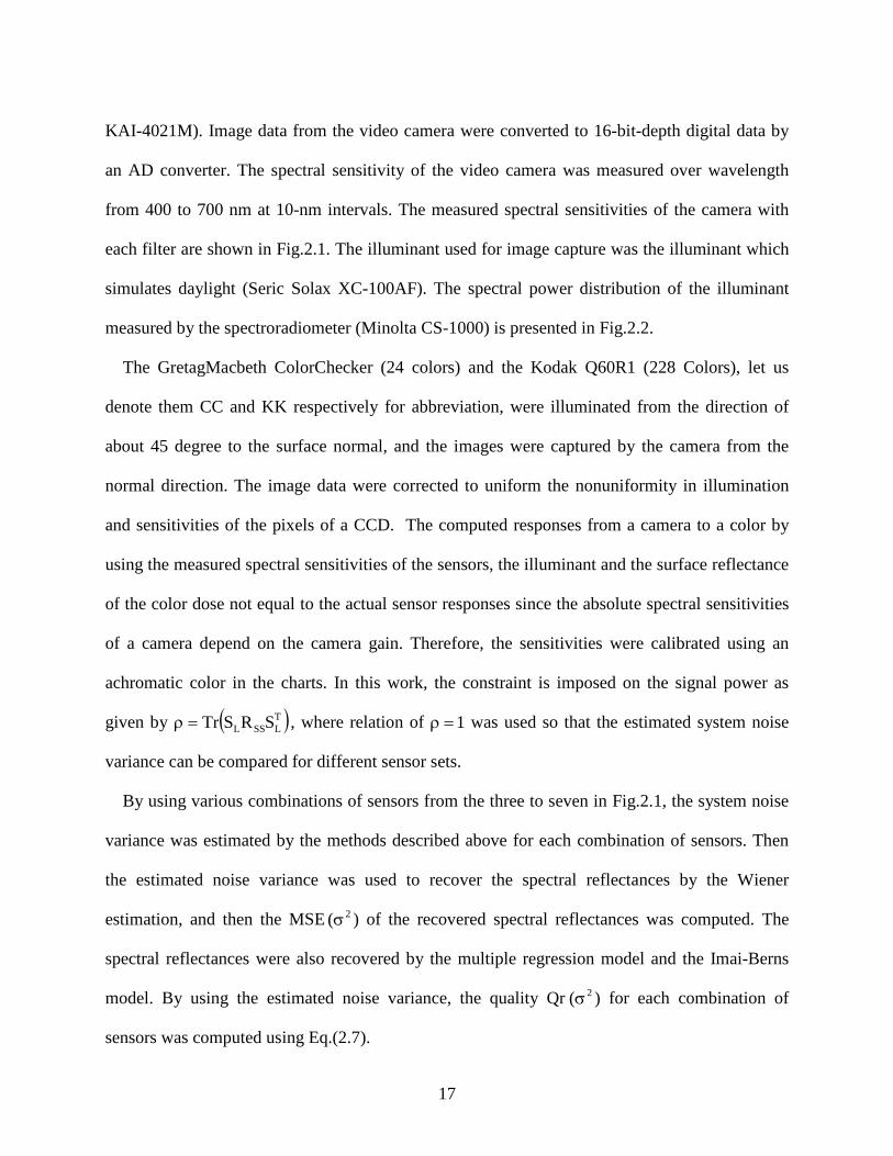
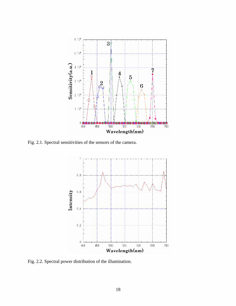
each filter are shown in Fig.2.1. The illuminant used for image capture was the illuminant which

simulates daylight (Seric Solax XC-100AF). The spectral power distribution of the illuminant

measured by the spectroradiometer (Minolta CS-1000) is presented in Fig.2.2.

The GretagMacbeth ColorChecker (24 colors) and the Kodak Q60R1 (228 Colors), let us

denote them CC and KK respectively for abbreviation, were illuminated from the direction of

about 45 degree to the surface normal, and the images were captured by the camera from the

normal direction. The image data were corrected to uniform the nonuniformity in illumination

and sensitivities of the pixels of a CCD. The computed responses from a camera to a color by

using the measured spectral sensitivities of the sensors, the illuminant and the surface reflectance

of the color dose not equal to the actual sensor responses since the absolute spectral sensitivities

of a camera depend on the camera gain. Therefore, the sensitivities were calibrated using an

achromatic color in the charts. In this work, the constraint is imposed on the signal power as

given by ( )TLSSL SRSTr=ρ , where relation of 1=ρ was used so that the estimated system noise

variance can be compared for different sensor sets.

By using various combinations of sensors from the three to seven in Fig.2.1, the system noise

variance was estimated by the methods described above for each combination of sensors. Then

the estimated noise variance was used to recover the spectral reflectances by the Wiener

estimation, and then the MSE )( 2σ of the recovered spectral reflectances was computed. The

spectral reflectances were also recovered by the multiple regression model and the Imai-Berns

model. By using the estimated noise variance, the quality Qr )( 2σ for each combination of

sensors was computed using Eq.(2.7).

18

Fig. 2.1. Spectral sensitivities of the sensors of the camera.

Fig. 2.2. Spectral power distribution of the illumination.

19

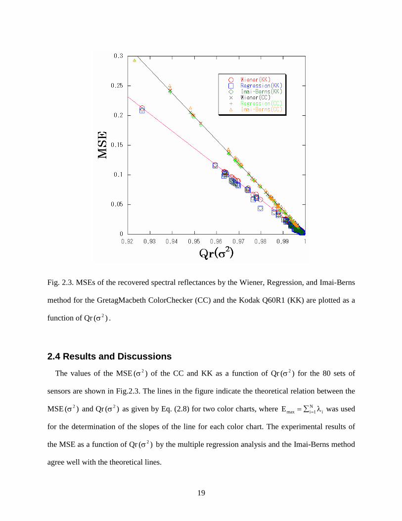
Fig. 2.3. MSEs of the recovered spectral reflectances by the Wiener, Regression, and Imai-Berns

method for the GretagMacbeth ColorChecker (CC) and the Kodak Q60R1 (KK) are plotted as a

function of Qr )( 2σ .

2.4 Results and Discussions

The values of the MSE )( 2σ of the CC and KK as a function of Qr )( 2σ for the 80 sets of

sensors are shown in Fig.2.3. The lines in the figure indicate the theoretical relation between the

MSE )( 2σ and Qr )( 2σ as given by Eq. (2.8) for two color charts, where iN

1imaxE λ∑= = was used

for the determination of the slopes of the line for each color chart. The experimental results of

the MSE as a function of Qr )( 2σ by the multiple regression analysis and the Imai-Berns method

agree well with the theoretical lines.

20

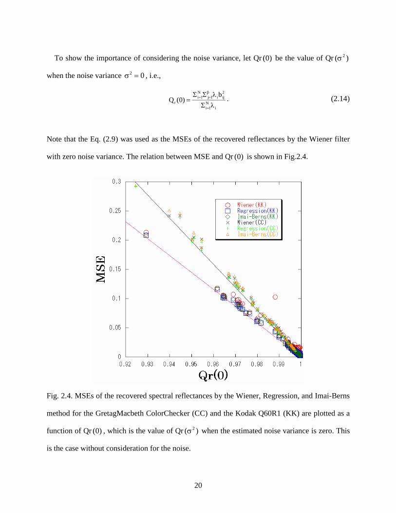
To show the importance of considering the noise variance, let Qr )0( be the value of Qr )( 2σ

when the noise variance 02 =σ , i.e.,

i

N1i

2iji1j

N1i

r

b)0(Q

λΣλΣΣ

==

β== . (2.14)

Note that the Eq. (2.9) was used as the MSEs of the recovered reflectances by the Wiener filter

with zero noise variance. The relation between MSE and Qr )0( is shown in Fig.2.4.

Fig. 2.4. MSEs of the recovered spectral reflectances by the Wiener, Regression, and Imai-Berns

method for the GretagMacbeth ColorChecker (CC) and the Kodak Q60R1 (KK) are plotted as a

function of Qr )0( , which is the value of Qr )( 2σ when the estimated noise variance is zero. This

is the case without consideration for the noise.

21

In Fig.2.4 plots not only disagree with the theoretical lines but also scatter more largely

compared to the Fig.2.3. Especially the plots of the KK recovered by the Wiener model scatter

far above the theoretical line. These scattered plots indicate the importance of the accurate

estimation of the noise variance in the images. Also we confirmed that plots of the CC scatter

more largely in Fig.2.4 when the 6-bit AD converter is used instead of the 16-bit converter to

digitize the sensor responses.

The results in Fig.2.3 agree well with the theoretical predictions and it means that Qr )( 2σ is

able to be used for the multiple regression analysis and the Imai-Berns model. As a matter of a

fact, the multiple regression model and the Imai-Berns model are mathematically equivalent to

the Wiener estimation, i.e., the matrixes W in Eq.(2.12) and B in Eq. (2.13) are equivalent to

the matrix of the Wiener filter 0W in Eq.(2.3) and which can be proved by the mathematical

analysis. For proofs of the equivalences, see the appendix.

Typical examples of the recovered reflectances and the reproduced color images for three

cases of the Qr )( 2σ are shown in Fig.2.5 through Fig.2.7. It is very clear that the error of the

recovered spectral reflectances increase with a decrease in the Qr )( 2σ and faithfulness of the

reproduced colors decreases with a decrease in the Qr )( 2σ . Also the typical examples of the

maximum and minimum values of the Qr )( 2σ and MSE )( 2σ by the three models for each

number (three to seven) of sensor sets are shown in Table 2.1. It is very interesting that a set of

four sensors (sensor number “2457”) has a larger Qr )( 2σ than a set of six sensors (sensor

number “123456”). It is not always true that the Qr )( 2σ increases when the number of the

sensors increases.

Though we confirmed that the Wiener model recovers the reflectances most accurately of the

three reflectance recovery models such as the Wiener, the regression and the Imai-Berns model

in most cases, especially in the cases when the reflectances of the learning sample and the test

22

sample are not similar [34] and that the Wiener model recovers the highly accurate reflectances

by selecting the appropriate learning samples from a group of samples or databases of

reflectances of objects [35], we have to recover the reflectances by the multiple regression model

or the Imai-Berns model when prior knowledge of the spectral sensitivities of a set of sensors or

the spectral power distribution of the illuminant are unknown. In other words, we have to

evaluate the image acquisition devices by the multiple regression model or the Imai-Berns model

when prior knowledge of the image acquisition device is unknown. It is now confirmed that the

MSE )( 2σ of the spectral reflectances recovered by the multiple regression model and the Imai-

Berns model have a linear relation to the quality Qr )( 2σ of the image acquisition system. Once

this linear relation is confirmed, we can estimate Qr )( 2σ by the multiple regression or the Imai-

Berns model without the spectral sensitivities of sensors, the spectral power distribution of the

recording illuminant or the noise present in the image acquisition system since it (Qr )( 2σ ) can

be easily estimated by marking the value of the MSE by the models on the theoretical line, i.e.,

the corresponding Qr )( 2σ of the point gives the estimate.

Now it is possible to estimate the quality Qr )( 2σ by the multiple regression model or the

Imai-Berns model with only the spectral reflectances and the captured images of the object.

2.5 Conclusions

The evaluation of an image acquisition system aimed at recovery of spectral reflectances,

which is derived based on the Wiener estimation, was applied to the multiple regression analysis

and the Imai-Berns method. The experimental results by multispectral cameras agree quite well

with the proposed model. From this result, it is concluded that the proposed evaluation model is

appropriately formulated and that the estimation of the noise variance of an image acquisition

system is essential to evaluate the quality Qr )( 2σ . This result also gives us an easy way to

23

estimate the quality Qr )( 2σ and provides us an easier way to evaluate an image acquisition

system aimed at reconstruction of spectral reflectances without the spectral sensitivities of

sensors, the spectral power distribution of the recording illuminant or the noise present in the

image acquisition system [36].

24

(a)

(b)

Fig. 2.5. (a) Typical example of the recovered spectral reflectance of the color red at a large

Qr )( 2σ (Qr )( 2σ = 0.996894). (b) Color reproduction of the GretagMacbeth ColorChecker by

the recovered spectral reflectance at Qr )( 2σ = 0.996894.

25

(a)

(b)

Fig. 2.6. (a) Typical example of the recovered spectral reflectance of the color red at a middle



26

(a)

(b)

Fig. 2.7. (a) Typical example of the recovered spectral reflectance of the color red at a small



27

Table 2.1. Maximum and minimum Qr )( 2σ for each number of sensors of the Macbeth

ColorChecker.

Qr )( 2σ Number

of sensors

Sensors Qr(0) MSE )( 2σ (Wiener)

MSE(0) MSE (Regression)

MSE (Imai-Berns)

0.996894 7ch 1234567 0.997397 0.012164 0.012423 0.010682 0.011500 0.996324 6ch 134567 0.996891 0.014354 0.014631 0.013326 0.014258 0.995627 5ch 13467 0.996312 0.017177 0.017348 0.016063 0.016816 0.993334 4ch 2457 0.993690 0.026408 0.026374 0.025583 0.026071 0.989134 6ch 123456 0.990872 0.043106 0.043771 0.037802 0.038943 0.987814 3ch 257 0.988318 0.048248 0.048213 0.047758 0.048249 0.923114 5ch 12345 0.924614 0.304426 0.304508 0.292043 0.293503 0.856650 4ch 1234 0.860630 0.569539 0.569701 0.558052 0.563130 0.787850 3ch 123 0.791501 0.838561 0.839893 0.817497 0.826465

28

References 1. P.S. Hung, “Colorimetric calibration for scanners and media,” Proc. SPIE 1448, 164-174

(1991).

2. H.R. Kang, “Colorimetric scanner calibration”, J. Imaging Sci. Technol. 36(2), 162-170

(1992).

3. G. Sharma and H.J. Trussell, “Figure of merit for color scanners,” IEEE Trans. Image

Process. 6(7), 990-1001 (1997).

4. N. Shimano, “Suppression of noise effect in color corrections by spectral sensitivities of

image sensors,” Opt. Rev. 9(2), 81-88 (2002).

5. S. Quan, N. Ohta, R.S. Berns, X. Jiang and N. Katoh, “Unified measure of goodness and

optimal design of spectral sensitivity functions,” J. Imaging Sci. Technol. 46(6), 485-497

(2002).

6. H.E.J. Neugebauer “Quality factor for filters whose spectral transmittances are different from

color mixture curves, and its application to color photography.” J. Opt. Soc. Am. 46(10),821-

824 (1956)

7. P.L. Vora and H.J. Trussell, “Measure of goodness of a set of color-scanning filters,” J. Opt.

Soc. Am. A 10(7), 1499-1508 (1993).

8. N. Shimano, "Optimization of spectral sensitivities with Gaussian distribution functions for a

color image acquisition device in the presence of noise", Optical Engineering, vol.45(1).,

pp.013201-1-8, (2006).

9. G. Sharma, H.J. Trussell and M.J. Vrhel, “Optimal nonnegative color scanning filters,” IEEE

Trans Image Process. 7(1), 129-133 (1998).

10. N. Shimano, "Recovery of Spectral Reflectances of Objects Being Imaged Without Prior

Knowledge" IEEE Trans. Image Process. vol. 15, no.7, pp. 1848-1856, Jul. (2006).

11. N. Shimano, “Application of a Colorimetric Evaluation Model to Multispectral Color Image

Acquisition Systems” J. Imaging Sci. Technol. 49(6), 588-593 (2005).

12. J. Cohen, "Dependency of spectral reflectance curves of the Munsell color chips", Psychon.

Sci, 1, 369-370(1964).

29

13. L. T. Maloney, "Evaluation of linear models of surface spectral reflectance with small

numbers of parameters", J. Opt. Soc. Am. A3, 1673-1683(1986).

14. J. P. S. Parkkinen, J. Hallikainen, T. Jaaskelainen, "Characteristic Spectra of Munsell Colors",

J. Opt. Soc. Am. A6, 318-322(1989).

15. J. L. Dannemiller, "Spectral reflectance of natural objects: how many basis functions are

necessary?" J. Opt. Soc. Am. A9, 507-515(1992).

16. A. Rosenfeld and A. C. Kak, Digital Picture Processing, 2nd ed., (Academic Press, 1982).

17. H. Haneishi, T. Hasegawa, N. A. Hosoi, Y. Yokoyama, N. Tsumura and Y. Miyake, "System

design for accurately estimating the spectral reflectance of art paintings", Appl. Optics,

39,6621-6632(2000).

18. Y. Zhao, L.A. Taplin, M. Nezamabadi and R.S. Berns, “Using the Matrix R Method for

Spectral Image Archives”, The 10th Congress of the International Color Association (AIC’5),

(Granada, Spain), pp.469-472 (2005).

19. K. Martinez, J. Cupitt, D. Saunders and R. Pillay, "Ten Years of Art Imaging Research",

Proc. of the IEEE, 90,28-41(2002).

20. A. A. Afifi and S. P. Azen, "Statistical Analysis", Chap.3,(Academic Press,1972).

21. H. L. Shen and H. H. Xin, "Spectral characterization of a color scanner based on optimized

adaptive estimation", J. Opt. Soc. Am. A23, 1566-1569(2006).

22. D. Connah, J. Y. Hardeberg, and S. Westland, "Comparison of Linear Spectral

Reconstruction Methods for Multispectral Imaging", Proc. IEEE's International Conference

on image Processing (IEEE,2004),pp.1497-1500.

23. Y. Zhao, L. A. Taplin, M. Nezamabadi, and R. S. Berns, "Methods of Spectral Reflectance

Reconstruction for A Sinarback 54 Digital Camera", Munsell Color Science Laboratory

Technical Report December 2004,pp.1-36(2004).

24. D. Connah and J. Y. Hardeberg, "Spectral recovery using polynomial models” Proc. SPIE

5667, 65-75 (2005)

25. J. L. Nieves, E. M. Valero, S. M. C. Nascimento, J. H. Andrés, and J. Romero, "Multispectral

synthesis of daylight using a commercial digital CCD camera", Appl. Optics, 44, 5696-

5703(2005).

30

26. F.H. Imai and R.S. Berns, "Spectral Estimation Using Trichromatic Digital Cameras", Proc.

Int. Symposium on Multispectral Imaging and Color Reproduction for Digital Archives,

Chiba, Japan. 42-49, (1999).

27. M. A. López-Álvarez, J. Hernández-Andrés, Eva. M. Valero and J. Romero, "Selecting

algorithms, sensors and liner bases for optimum spectral recovery of skylight" J. Opt. Soc.

Am. A24,942-956(2007).

28. V. Cheung, S. Westland, C. Li, J. Hardeberg and D. Connah, "Characterization of

trichromatic color cameras by using a new multispectral imaging technique", J. Opt. Soc. Am.

A22, 1231-1240(2005).

29. M. Shi and G. Healey, “Using reflectance models for color scanner calibration”, J. Opt. Soc.

Am. A 19(4), 645-656 (2002).

30. Y. Miyake and Y. Yokoyama, "Obtaining and Reproduction of Accurate Color Images Based

on Human Perception", Proc. SPIE 3300, 190-197(1998).

31. N. Shimano, "Evaluation of a multispectral image acquisition system aimed at reconstruction

of spectral reflectances", Optical Engineering, vol.44, pp.107115-1-6, (2005).

32. M. Hironaga, K. Terai and N. Shimano, “A model to evaluate color image acquisition

systems aimed at the reconstruction of spectral reflectances”, Proc. Ninth International

Symposium on Multispectral Color Science and Application, Taipei, R.O.C. 23-28, (2007).

33. G.H. Golub and C.F.V. Loan, "Matrix Computations", The Johns Hopkins

34. N. Shimano, K. Terai, and M. Hironaga, "Recovery of spectral reflectances of objects being

imaged by multispectral cameras," J. Opt. Soc. Am. A 24, 3211-3219 (2007).

35. N. Shimano and M. Hironaga, "Recovery of spectral reflectances of imaged objects by the

use of features of spectral reflectances," J. Opt. Soc. Am. A 27, 251-258 (2010).



030503(2008).

31

Appendix

A. Proof of the equivalence of the multiple regression model to the Wiener model.

The multiple regression model minimizes

WPR − , (A2.1)

where P is a kM× matrix which contains the sensor response vectors k21 ,,, ppp and let R be

a kN× matrix which contains the corresponding spectral reflectances vectors k21 ,,, rrr , where

k is the number of the learning samples. The MN× matrix W which minimizes Eq.(A2.1) is

given by

+= RPW , (A2.2)

where +P represents the pseudo inverse matrix of the matrix P .

1TT )PP(PP −+ = (A2.3)

because kM < holds in the image acquisition devices and M)P(Rank = . Let

ERSLP += , (A2.4)

where S is a NM× matrix of the spectral sensitivities of sensors in which a row vector

represents a spectral sensitivity, L is an NN× diagonal matrix with samples of the spectral

power distribution of an illuminant along the diagonal, and E is a NM× matrix which contains

the additive noise vectors. For abbreviation, let SLSL = . Substitution of Eq. (A2.3) and Eq.

(A2.4) into Eq. (A2.2) leads to

1TLL

TL ))ERS)(ERS(()ERS(RW −+++= . (A2.5)

32

Hence W is rewritten as

( ) 12e

TLL

TL IRssSSRssSW −

σ+= (A2.6)

because tRR is an autocorrelation matrix of R and tEE gives the noise variance and

0ERRE TT == as the spectral reflectances and the error have no correlation.

Thus the matrix W is equivalent to that of the Wiener filter.

B. Proof of the equivalence of the Imai-Berns model to the Wiener model.

Let Σ be a kd× matrix which contains the vectors of the weights to represent the k known

spectral reflectances, where d is a number of the weights to represent the spectral reflectances

and let P , R , LS and E be as defined in Appendix A.

A Md× matrix B which minimizes

BP=Σ (B2.1)

is given by

+Σ= PB . (B2.2)

From the Eq. (A2.2) through (A2.6), it is easily understood that

1TTL

TL

TTL

T )EESRRS)(ESR(VPVVB −+ ++Σ=Σ= . (B2.3)

From the definition of the method, Σ= VR , where V is an orthonormal basis matrix. Hence

( ) 12e

TLL

TL IRssSSRssSVB −

σ+= . (B2.4)

Thus the Imai-Berns model is equivalent to the Wiener Model.

33

Chapter 3

Noise robustness of a colorimetric evaluation model for

image acquisition devices with different characterization

models

A colorimetric evaluation of an image acquisition device is important for evaluating and

optimizing a set of sensors. Shimano proposed a colorimetric evaluation model [J. Imaging

Sci. Technol. 49(6), 588-593 (2005)] based on the Wiener estimation. The mean square

errors (MSE) between the estimated and the actual fundamental vectors by the Wiener

filter and the proposed colorimetric quality (Qc) agreed quite well with the proposed model

and he showed that the estimation of the system noise variance of the image acquisition

system is essential for the evaluation model.

In this chapter, it is confirmed that the proposed model can be applied to two different

reflectance recovery models and these models provide us an easy method for estimating

the proposed colorimetric quality (Qc). The system noise originates from the sampling

errors of the spectral characteristics of the sensors, the illuminations and the reflectance

and the quantization errors. The influence of the system noise on the evaluation model is

studied and it is confirmed from the experimental results that the proposed model holds

even in a noisy condition.

34

3.1 Introduction

Evaluating a color acquisition device is essential for designing optimum sets of sensors. There

are two approaches to evaluate a color acquisition device, one is the spectral evaluation and the

other is the colorimetric evaluation. These two approaches of the evaluation have each specific

purpose.

In the spectral evaluation, the main purpose of the image acquisition device is to obtain the

accurate spectral reflectances of objects being imaged in reproducing a color image under a

variety of viewing illuminants [1]. The accuracy of the recovered spectral reflectances depends

on the number of sensors, their spectral sensitivities, the objects being imaged, the recording

illuminants, the noise present in a device and the model used for the recovery. To obtain the

spectral reflectances of the imaged objects through the use of sensor responses, several models,

such as the Wiener model [2], the multiple regression model [3-10], the Imai-Berns model

[11-13] and the Shi-Healey model [14], and the linear model [15-17] have been studied. The

optimizations of spectral sensitivities for the acquisition of accurate spectral information of

objects are also reported [2,18,19]. Some papers on the optimization of spectral sensitivities for

the acquisition of spectral power distributions of illuminants have also been presented [10,12].

On the other hand in colorimetric evaluation, the main purpose of the image acquisition device

is to estimate the accurate colorimetric values of the pixels of objects being imaged [20,21]. The

accuracy of the estimates depends on the spectral sensitivities of a set of sensors, the objects

being imaged, the recording and viewing illuminants, the colorimetric characterization and the

noise present in the device. In the past, several models have been proposed to evaluate a

colorimetric performance of a set of color sensors. Neugebauer proposed a colorimetric quality

factor for the evaluation of a single sensor [22] and Vora and Trussell developed a model to

evaluate a set of sensors for the first time [23]. However, the Vora-Trussell model used a random

35

variable assumption of a surface reflectance. Since a surface spectral reflectance is smooth over

the visual wavelengths and falls into a subspace spanned by a small set of basis vectors, their

assumption was not adequate. Later, Sharma and Trussell reported a comprehensive analysis to

establish the colorimetric quality of an image acquisition device by taking account of the noise

effects and statistical properties of spectral reflectance of samples in the tristimulus values, the

orthogonal color space and the linearized CIELAB color space [24]. However, the formula by

Sharma and Trussell was too complicated to give an intuitive insight into the influence of the

noise on color correction and to predict new phenomena. Shimano proposed a simple formula to

evaluate colorimetric quality of a set of color sensors by considering the statistical properties of

spectral reflectance of samples and noise [25]. By the use of the evaluation models, the

optimization of a set of sensors has been performed [26,27]. However, the application of the

evaluation models to real color image acquisition devices has not appeared because of the

difficulty in estimating noise levels. Recently Shimano proposed a new model to estimate the

noise variance of an image acquisition system and applied it to the proposed colorimetric

evaluation model [25,28] and spectral evaluation model [29], and confirmed that the both

evaluation models agree quite well with the experimental results by multispectral cameras.

For a colorimetric evaluation, color stimuli can be divided into two parts, the fundamental and

the residual [30]. The fundamental is a projection of a color stimulus onto the human visual

subspace (HVSS) and evokes color sensation to human visual system. The residual is an

orthogonal part of the color stimulus and evokes no sensation. In the proposed colorimetric

evaluation model, the colorimetric quality Qc is related with the mean square errors (MSE)

between the estimated and measured fundamental vectors [31] that are the reflectance vectors

projected onto the HVSS. The proposed colorimetric evaluation model is formulated by

( ))(Q1E)(MSE 2cmax

2 σ−=σ , where MSE )( 2σ is the mean square errors between the recovered

36

and measured fundamental vectors with the estimated noise variance )( 2σ , Emax represents a

constant that is determined by the viewing illuminant, the CIE color matching functions and the

spectral reflectances of objects and Qc )( 2σ is the colorimetric quality of the image acquisition

system with the estimated noise variance 2σ . It was shown that Qc )( 2σ is determined by the

spectral sensitivities of the sensors, the spectral power distribution of the recording and viewing

illuminants, the noise variance of the image acquisition device and the spectral reflectances of

the imaged objects. The model was applied to the multispectral cameras and it was confirmed

that the model agrees quite well with the experimental results, i.e., the MSE )( 2σ of the

recovered fundamental vectors and the colorimetric quality Qc )( 2σ of a set of sensors showed a

predicted formulation of ( ))(Q1E)(MSE 2cmax

2 σ−=σ . As Qc )( 2σ is derived from Wiener

estimation [32], it is very important to confirm whether the model can be applied to other

recovery models since the colorimetric quality Qc )( 2σ is useful not only for the colorimetric

evaluation of an image acquisition device but also for the colorimetric optimization of a set of

sensors. In our recent study, we have shown that the quality Qr )( 2rσ of a set of sensors aimed at

recovery of spectral reflectances proposed by us can be applied to three different reflectance

recovery models [33], where 2rσ is the noise variance estimated from the spectral reflectances

[34]. But Qr )( 2rσ derived from the reflectance recovery model has little correlation with the

colorimetric quality Qc )( 2σ . For the colorimetric evaluation, it is required to examine that these

reflectance recovery models can be applied to the colorimetric quality Qc )( 2σ in the human

visual subspace spanned by the color matching functions or spectral sensitivities of cones.

In this chapter, it is shown that the relation between Qc )( 2σ and MSE )( 2σ shows the

theoretical prediction of MSE )( 2σ =Emax(1-Qc )( 2σ ), where the MSE )( 2σ is the mean square

error of the fundamental vectors recovered by the multiple regression analysis [3-10] and the

Imai-Berns model [11-13] by experiments, and the influence of the sampling intervals and the

37

quantization error of the image data on the evaluation model is examined. From the experimental

results, it is confirmed that even in the low signal-to-noise ratio (SNR) conditions, the Qc )( 2σ is

also appropriately formulated for these models. Once this linear relation is confirmed, we can

estimate Qc )( 2σ by the values of the MSE )( 2σ by the multiple regression model or the Imai-

Berns model, without knowing the spectral sensitivities of the sensors, spectral power

distribution of recording illuminant or estimating the noise variance and this relation provides us

an easier way for the colorimetric evaluation of a real existing image acquisition system.

This chapter is organized as follows. The outline of the colorimetric evaluation model and the

models tested are briefly reviewed in section 3.2. In section 3.3, the experimental procedures and

the results to demonstrate the trustworthiness of the proposal are described. The final section

presents the conclusions.

3.2 Models for the Colorimetric Evaluation

In this section, the derivation of the colorimetric quality Qc )( 2σ to evaluate the color image

acquisition system and the models used for the experiments are briefly reviewed.

3.2.1 Wiener Estimation Using Estimated Noise Variance

The visible wavelengths from 400 to 700 nm are sampled at a constant intervals and the

number of the samples is denoted as N. A sensor response vector from a set of color sensors for

an object with a 1N× spectral reflectance vector r can be expressed by

erp += oSL , (3.1)

where p is a 1M× sensor response vector from the M channel sensors, S is a NM× matrix of

the spectral sensitivities of sensors in which a row vector represents a spectral sensitivity, oL is a

NN× diagonal matrix with samples of the spectral power distribution of an recording illuminant

38

along the diagonal, and e is a 1M× additive noise vector. The noise e is defined to include all

the sensor response errors such as the measurement errors in the spectral characteristics of

sensitivities, an illumination and reflectances, and quantization errors in this work and it is

termed as the system noise [33] below. The system noise is assumed to be signal independent,

zero mean and uncorrelated to itself. For abbreviation, let oL SLS = . Denote the projection

matrix into the HVSS as VP which is represented by Tii

1iVP aa

α

=∑= , where ia is the i-th

orthonormal basis vector which spans HVSS and )TL(Rank V=α . { } α= ,,1ii a are the right

singular vectors determined by the singular value decomposition (SVD) of the matrix VTL ,

where T is the N3× matrix of CIE color matching functions and VL is an NN× diagonal

matrix with samples of the spectral power distribution of a viewing illuminant along the diagonal.

The projected vector rVP is termed a fundamental vector [25,28]. If r represents the recovered

spectral reflectance, the mean square errors (MSE) between the actual fundamental vector rVP

and the recovered fundamental vector rPV is given by

{ }2VV ˆPPEMSE rr −= , (3.2)

where { }•E represents the expectation. By the Wiener estimation, the matrix 0W which gives the

estimated spectral reflectance pr 0Wˆ = is given by

( ) 12e

TLL

TL0 IRssSSRssSW −

σ+= , (3.3)

where superscripted T represents the transpose of a matrix, Rss is an autocorrelation matrix of

the spectral reflectance of samples that will be captured by a device, and 2eσ is the noise variance

used for the estimation. Denote the actual system noise variance expressed as 2σ . If 2eσ is equal

to 2σ , substitution of Eq.(3.3) into Eq.(3.2) leads to [25,28,33]

39

( )2vi

Tvj22v

j

2

1j1i

2viCV

1i

2vi

1i

2 P)(MSE abaaσ+κ

σ∑∑+∑−∑=σβ

=

α

=

α

=

α

=, (3.4)

where vib , v

jκ and β represent the i-th right singular vector, j-th singular value and a rank of a

matrix 2/1LVS Λ , respectively. The column vector v

ia is given by iT2/1v

i V aa Λ= , Rss is

represented as TVVRss Λ= , where V is a basis matrix and Λ is a NN× diagonal matrix with

positive eigenvalues iλ along the diagonal in decreasing order, CVP is the projection matrix onto

the subspace spanned by a set of basis vectors { } β= ,,1ivi

b and represented by Tvi

vi

1iCVP bb

α

=∑= .

The first and second terms on the right-hand side of the Eq.(3.4) represent the MSE for the

noiseless case, which is denoted as MSEfree

2viCV

1i

2vi

1ifree PMSE aa

α

=

α

=∑−∑= , (3.5)

and the third term corresponds to the increase in the MSE due to the presence of the noise, which

is denoted as Noise Influence Factor (NIF) below.

( )2vi

Tvj22v

j

2

1j1iNIF ab

σ+κ

σ∑∑=β

=

α

=. (3.6)

Therefore the colorimetric quality of a set of color sensors in the presence of noise is formulated

as

( )

2vi

1i

2vi

Tvj22v

j

2

1j1i

2viCV

1i2

c

P

)(Qa

aba

α

=

β

=

α

=

α

=

∑

σ+κ

σ∑∑−∑

=σ . (3.7)

Hence, the MSE )( 2σ is expressed as

40

( ))(Q1E)MSE( 2cmax

2 σ−=σ , (3.8)

where 2v

i1i

maxE aα

=∑= . This equation shows that the MSE )( 2σ has a linear relation to Qc )( 2σ

and the slope of the line is 2v

i1i

aα

=∑ . The values of

2vi

1ia

α

=∑ are dependent only on the viewing

illuminant, the CIE color matching functions and the surface spectral reflectance of the objects

being captured. The MSE )( 2σ decreases as the Qc )( 2σ increases to one.

The first term on the right-hand side of the Eq.(3.4), 2v

i1i

aα

=∑ , is considered to represent the

Statistical Mean Energy of Color Stimuli (SMECS) which is incident on the cones. The second

term on the right-hand side of the Eq.(3.4) represents the energy of the SMECS captured by a set

of color sensors. And the third term of it corresponds to the increase in the MSE due to the

presence of the noise [25]. Therefore, the colorimetric quality Qc )( 2σ in Eq.(3.7) can be

interpreted as the ratio of the energy a set of sensor capture to that of the SMECS.

If we let the noise variance 02e =σ for the Wiener filter in Eq.(3.3), then the MSE )0( is

derived as

( )2vi

Tvj2v

j

2

1j1i

2viCV

1i

2vi

1iP)0(MSE abaa

κ

σ∑∑+∑−∑=β

=

α

=

α

=

α

=

, (3.9)

where details of the proofs are shown in the previous paper [28].

Then the estimated system noise variance 2σ can be represented by

( )( )

2vj

2vi

Tvj

1j1i

free2 MSE0MSEˆ

κ∑∑

−=σ

β

=

α

=

ab. (3.10)

Therefore, the system noise variance 2σ can be estimated using Eq.(3.10), since the MSEfree

and the denominator of Eq.(3.10) can be computed if the surface reflectance spectra of objects,

41

the spectral sensitivities of sensors and the spectral power distribution of the recording and

viewing illuminants are known. The MSE )0( can also be obtained by the experiment using Eqs.

(3.2) and (3.3) applying the Wiener filter with 02e =σ to sensor responses. [25,28]

The colorimetric quality Qc )( 2σ and MSE )( 2σ can be computed by substituting the

estimated noise variance to Eq.(3.7) and Eq.(3.2) , respectively.

3.2.2 Application of the Multiple Regression Analysis to Fundamental Vector Evaluation

To achieve the colorimetric evaluation, the multiple regression model is used to recover the

fundamental vectors. Let ip be a 1M× sensor response vector which is obtained by the image

acquisition of a known spectral reflectance ir of the i-th object. Let P be a kM× matrix which

contains the sensor responses k21 ,,, ppp , and let F be a kN× matrix which contains the

corresponding fundamental vectors k21 ,,, fff , where iVi P rf = and k is the number of the

learning samples. The matrix W which minimizes WPF − , where notation • represents the

Frobenius norm[35] is given by.

+= FPW , (3.11)

where +P represents the pseudo inverse matrix of the matrix P . The estimated fundamental

vector if is given by ii Wˆ pf = . Therefore this model does not use the spectral sensitivities of

sensors or the spectral power distribution of an illumination, but it uses only the fundamental

vectors of the learning samples.

3.2.3 Application of the Imai-Berns Model to Fundamental Vector Evaluation

To achieve the colorimetric evaluation, the Imai-Berns model is applied to estimate the weight

matrix in the HVSS and is used to recover the fundamental vectors. The sensor response matrix

42

P and the fundamental vectors if =are defined the same manner as the regression model. Let Σ be

a kd× matrix which contains the column vectors of the weights k21 ,,, σσσ to represent the k

known fundamental vectors k21 ,,, fff , where d is a number of the weights. The multiple

regression analysis between Σ and P is expressed as BP−Σ . A matrix B which minimize the

Frobenius norm is given by

+Σ= PB . (3.12)

Since a weight column vectors iσ for a sensor response vector ip is estimated by ii Bˆ pσ = ,

the estimated fundamental vector is derived from ii ˆVˆ σf = , where a matrix V is the basis matrix

which contains first d orthonormal basis of the fundamental vectors. This model does not use the

spectral characteristics of sensors or an illumination.


Detailed experimental procedures and conditions are described in the previous paper [33,34]

and the procedures specific to this chapter are described briefly below.



KAI-4021M). The images of a GretagMacbeth ColorChecker (24 colors) and the Kodak Q60R1

(228 Colors), let us denote them CC and KK respectively for abbreviation, were converted to 16-

bit-depth digital data by an AD converter. The spectral reflectances of the GretagMacbeth

ColorChecker, spectral characteristics of the illumination and the sensors of the camera were

measured at 1-nm sampling intervals over wavelength from 400 to 700 nm (Kodak Q60R1 were

only measured at 10-nm sampling intervals). Next the least significant bits of the measured 16-

bit image data are taken away to simulate various quantization errors and the spectral

43

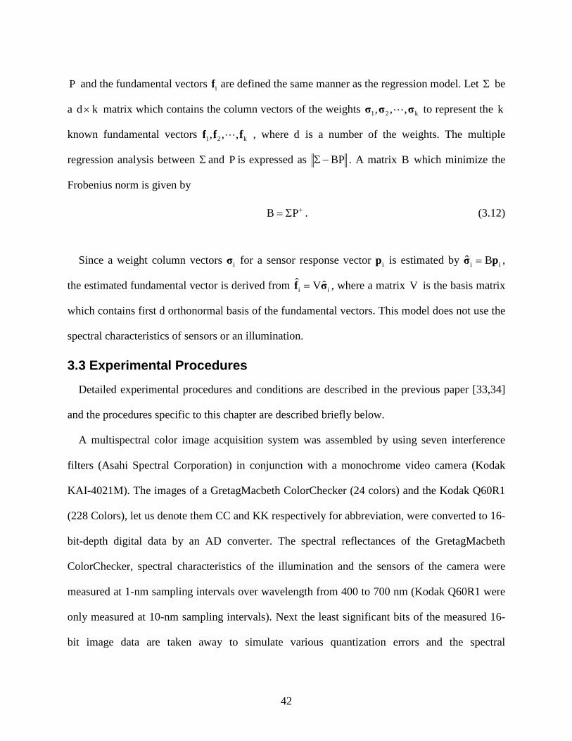
characteristics are converted to desired sampling intervals. The measured spectral sensitivities of

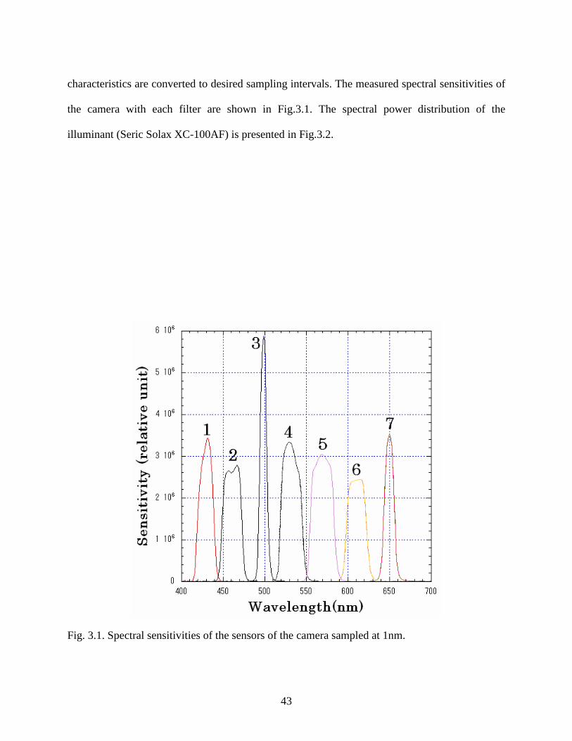
the camera with each filter are shown in Fig.3.1. The spectral power distribution of the

illuminant (Seric Solax XC-100AF) is presented in Fig.3.2.

Fig. 3.1. Spectral sensitivities of the sensors of the camera sampled at 1nm.

44

Fig. 3.2. Spectral power distribution of the illumination sampled at 1nm.

By using all combinations of sensors from three to seven sensors sampling at various sampling

intervals and the signals with various sampling bit depth, the system noise variance was

estimated and the colorimetric quality Qc )( 2σ was computed. Then the estimated noise variance

was used to recover the fundamental vectors with the spectral reflectance recovered by the

Wiener estimation, and then the MSE )( 2σ of the recovered fundamental vectors was computed

by averaging the difference between actual and recovered fundamental vectors over colors. The

fundamental vectors were also recovered by the multiple regression model and the Imai-Berns

model and MSE of the recovered fundamental vectors by theses models were computed. By

using the estimated noise variance, the colorimetric quality Qc )( 2σ for each combination of

sensors was computed using Eq.(3.7).

45

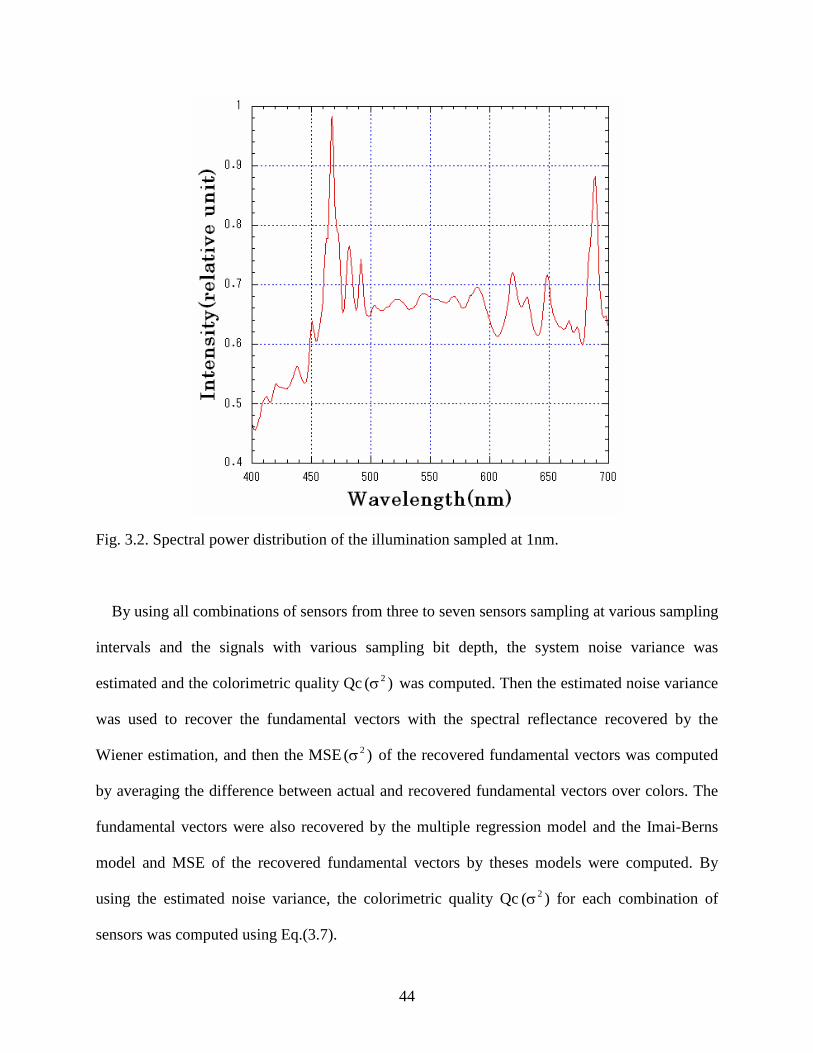
Fig. 3.3. MSEs of the recovered fundamental vectors by the Wiener, Regression, and Imai-Berns

model for the GretagMacbeth ColorChecker (CC) and the Kodak Q60R1 (KK) are plotted as a

function of Qc )( 2σ .


In this chapter, the learning sample is the same as the test sample, i.e. , if the test sample is CC

then the CC is used as the learning sample.

3.4.1 MSE and Qc )( 2σ

The plots of the MSE )( 2σ of the CC and KK as a function of Qc )( 2σ with 16-bit image and

10-nm sampling intervals for the spectral characteristics of the sensors, the illuminations and the

reflectance (16bit-10nm) are shown in Fig.3.3. The lines in the figure show the theoretical

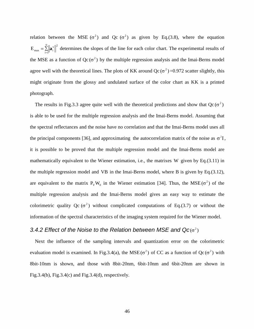
46

relation between the MSE )( 2σ and Qc )( 2σ as given by Eq.(3.8), where the equation 2v

i1i

maxE aα

=∑= determines the slopes of the line for each color chart. The experimental results of

the MSE as a function of Qc )( 2σ by the multiple regression analysis and the Imai-Berns model

agree well with the theoretical lines. The plots of KK around Qc )( 2σ =0.972 scatter slightly, this

might originate from the glossy and undulated surface of the color chart as KK is a printed

photograph.

The results in Fig.3.3 agree quite well with the theoretical predictions and show that Qc )( 2σ

is able to be used for the multiple regression analysis and the Imai-Berns model. Assuming that

the spectral reflectances and the noise have no correlation and that the Imai-Berns model uses all

the principal components [36], and approximating the autocorrelation matrix of the noise as I2σ ,

it is possible to be proved that the multiple regression model and the Imai-Berns model are

mathematically equivalent to the Wiener estimation, i.e., the matrixes W given by Eq.(3.11) in

the multiple regression model and VB in the Imai-Berns model, where B is given by Eq.(3.12),

are equivalent to the matrix 0VWP in the Wiener estimation [34]. Thus, the MSE )( 2σ of the

multiple regression analysis and the Imai-Berns model gives an easy way to estimate the

colorimetric quality Qc )( 2σ without complicated computations of Eq.(3.7) or without the

information of the spectral characteristics of the imaging system required for the Wiener model.

3.4.2 Effect of the Noise to the Relation between MSE and Qc )( 2σ

Next the influence of the sampling intervals and quantization error on the colorimetric

evaluation model is examined. In Fig.3.4(a), the MSE )( 2σ of CC as a function of Qc )( 2σ with

8bit-10nm is shown, and those with 8bit-20nm, 6bit-10nm and 6bit-20nm are shown in

Fig.3.4(b), Fig.3.4(c) and Fig.3.4(d), respectively.

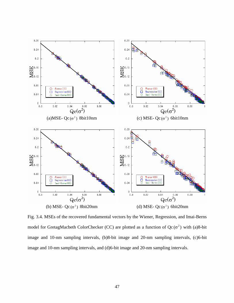
47

(a)MSE- Qc )( 2σ 8bit10nm

(b) MSE- Qc )( 2σ 8bit20nm

(c) MSE- Qc )( 2σ 6bit10nm

(d) MSE- Qc )( 2σ 6bit20nm


model for GretagMacbeth ColorChecker (CC) are plotted as a function of Qc )( 2σ with (a)8-bit

image and 10-nm sampling intervals, (b)8-bit image and 20-nm sampling intervals, (c)6-bit

image and 10-nm sampling intervals, and (d)6-bit image and 20-nm sampling intervals.

48

In Fig.3.4(b), although the plots for 8bit-20nm scatter slightly compared to those for 8bit-

10nm, the results agree fairly well with the theoretical line. In Fig.3.4(c) and Fig.3.4(d), the plots

for 6bit-10nm and 6bit-20nm are still along the theoretical line but they scatter largely compared

to those for 8bit-10nm because the system noise variance increases with the larger quantization

error or the larger sampling intervals. It is remarkable that the MSE )( 2σ and Qc )( 2σ still show

the relation of ( ))(Q1E)(MSE 2cmax

2 σ−=σ even with 6bit-20nm.


model for GretagMacbeth ColorChecker (CC) are plotted as a function of Qc )0( with 6-bit image

and 10-nm sampling intervals (MSE )0( s are plotted for the Wiener model).

49

To examine the effect of the estimation of the system noise variance, let Qc )0( be the value of

Qc )( 2σ when the noise variance is not considered, i.e.,

2v

i1i

2viCV

1ic

P)0(Q

a

aα

=

α

=

∑

∑= . (3.13)

The experimental results on the relation between Qc )0( and MSE )0( correspond to the case

where the noise present in the image acquisition device is not taken into account, which are

shown with 6bit-10nm in Fig.3.5. The MSE )0( can be obtained by the experiment using Eqs.

(3.2) and (3.3) applying the Wiener filter with 02e =σ . In Fig.3.5, the plots scatter largely far

above the theoretical line. Therefore, this result shows the importance of the estimation of the

noise variance in the evaluation model.

3.4.3 Effect of the Sampling Bits to MSE

Since the plots with 6bit-10nm scatters more than those with 8bit-20nm, to examine the effect

of the quantization error to the evaluation model, the most and least quantization error sensitive

sensor sets with 10-nm sampling interval are selected by the increase in the absolute error to the

theoretical MSE which is calculated by the Eq.(3.8) for 8-bit and 6-bit image. The sensor set

“247” has the least increase in the absolute error and the sensor set “1234” has the most increase

in the absolute error when quantization error is increased by changing the image data from 8-bit

to 6-bit. It is interesting to see that the least quantization error sensitive sensor set “247” has little

decrease in the colorimetric quality Qc )( 2σ , which is 0.988979 for 8-bit image and 0.987561 for

6-bit image, and the most quantization error sensitive sensor set “1234” has a large decrease in

the colorimetric quality Qc )( 2σ ,which is 0.923537 for 8-bit image and 0.903407 for 6-bit image.

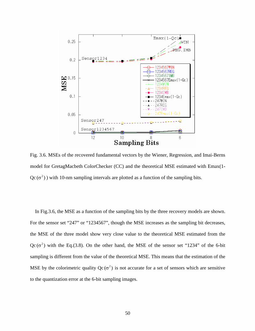
50


model for GretagMacbeth ColorChecker (CC) and the theoretical MSE estimated with Emax(1-

Qc )( 2σ ) with 10-nm sampling intervals are plotted as a function of the sampling bits.

In Fig.3.6, the MSE as a function of the sampling bits by the three recovery models are shown.

For the sensor set “247” or “1234567”, though the MSE increases as the sampling bit decreases,

the MSE of the three model show very close value to the theoretical MSE estimated from the

Qc )( 2σ with the Eq.(3.8). On the other hand, the MSE of the sensor set “1234” of the 6-bit

sampling is different from the value of the theoretical MSE. This means that the estimation of the

MSE by the colorimetric quality Qc )( 2σ is not accurate for a set of sensors which are sensitive

to the quantization error at the 6-bit sampling images.

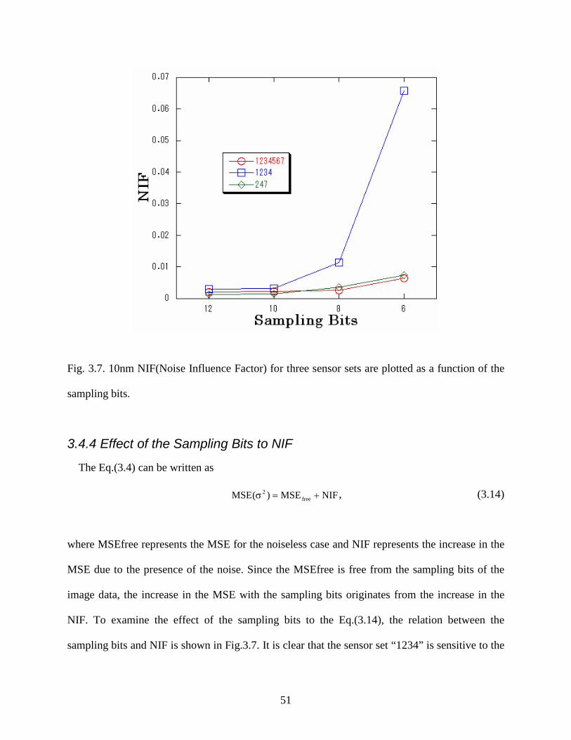
51

Fig. 3.7. 10nm NIF(Noise Influence Factor) for three sensor sets are plotted as a function of the

sampling bits.

3.4.4 Effect of the Sampling Bits to NIF

The Eq.(3.4) can be written as

NIFMSE)(MSE free2 +=σ , (3.14)

where MSEfree represents the MSE for the noiseless case and NIF represents the increase in the

MSE due to the presence of the noise. Since the MSEfree is free from the sampling bits of the

image data, the increase in the MSE with the sampling bits originates from the increase in the

NIF. To examine the effect of the sampling bits to the Eq.(3.14), the relation between the

sampling bits and NIF is shown in Fig.3.7. It is clear that the sensor set “1234” is sensitive to the

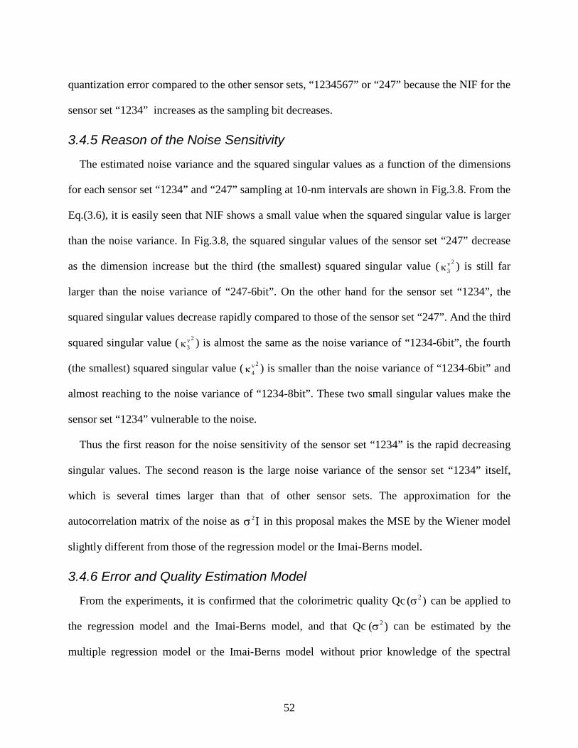
52

quantization error compared to the other sensor sets, “1234567” or “247” because the NIF for the

sensor set “1234” increases as the sampling bit decreases.

3.4.5 Reason of the Noise Sensitivity

The estimated noise variance and the squared singular values as a function of the dimensions

for each sensor set “1234” and “247” sampling at 10-nm intervals are shown in Fig.3.8. From the

Eq.(3.6), it is easily seen that NIF shows a small value when the squared singular value is larger

than the noise variance. In Fig.3.8, the squared singular values of the sensor set “247” decrease

as the dimension increase but the third (the smallest) squared singular value ( 2v3κ ) is still far

larger than the noise variance of “247-6bit”. On the other hand for the sensor set “1234”, the

squared singular values decrease rapidly compared to those of the sensor set “247”. And the third

squared singular value ( 2v3κ ) is almost the same as the noise variance of “1234-6bit”, the fourth

(the smallest) squared singular value ( 2v4κ ) is smaller than the noise variance of “1234-6bit” and

almost reaching to the noise variance of “1234-8bit”. These two small singular values make the

sensor set “1234” vulnerable to the noise.

Thus the first reason for the noise sensitivity of the sensor set “1234” is the rapid decreasing

singular values. The second reason is the large noise variance of the sensor set “1234” itself,

which is several times larger than that of other sensor sets. The approximation for the

autocorrelation matrix of the noise as I2σ in this proposal makes the MSE by the Wiener model

slightly different from those of the regression model or the Imai-Berns model.

3.4.6 Error and Quality Estimation Model

From the experiments, it is confirmed that the colorimetric quality Qc )( 2σ can be applied to

the regression model and the Imai-Berns model, and that Qc )( 2σ can be estimated by the

multiple regression model or the Imai-Berns model without prior knowledge of the spectral

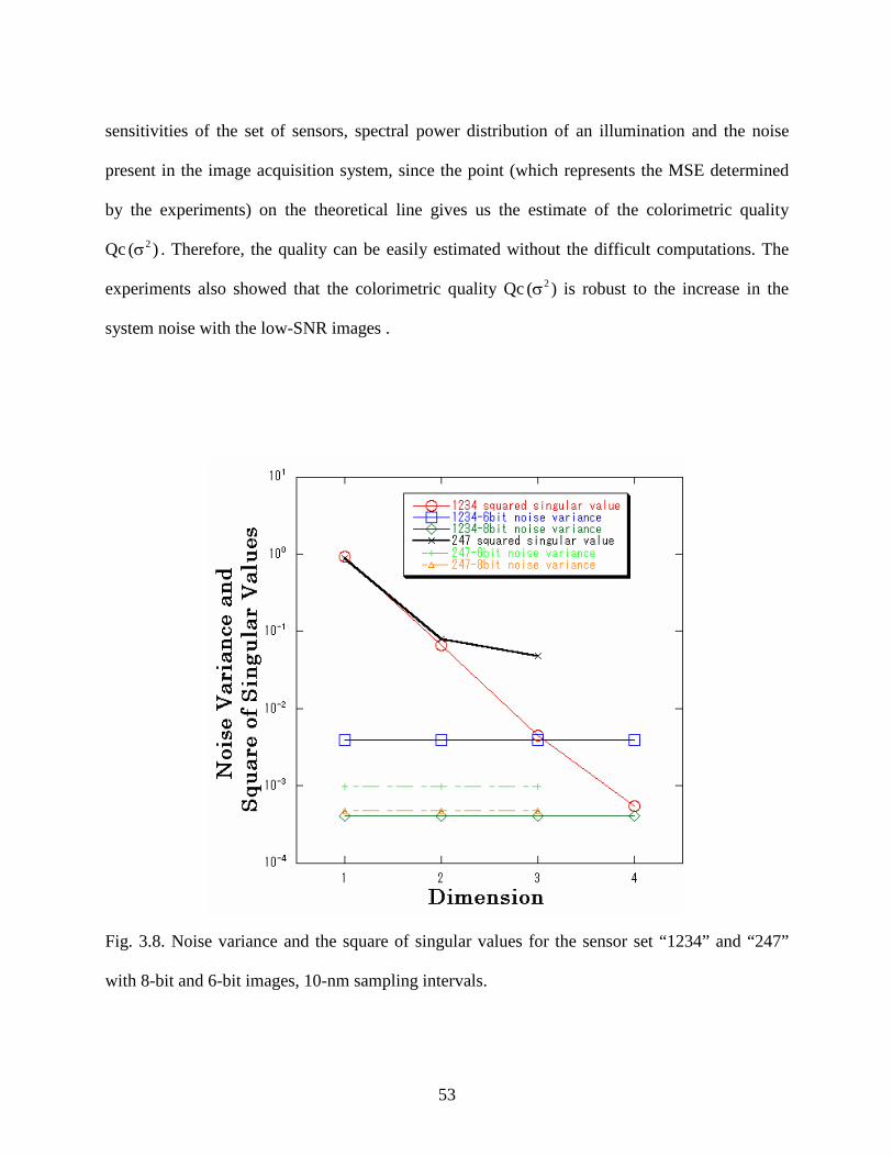
53

sensitivities of the set of sensors, spectral power distribution of an illumination and the noise

present in the image acquisition system, since the point (which represents the MSE determined

by the experiments) on the theoretical line gives us the estimate of the colorimetric quality

Qc )( 2σ . Therefore, the quality can be easily estimated without the difficult computations. The

experiments also showed that the colorimetric quality Qc )( 2σ is robust to the increase in the

system noise with the low-SNR images .

Fig. 3.8. Noise variance and the square of singular values for the sensor set “1234” and “247”

with 8-bit and 6-bit images, 10-nm sampling intervals.

54

3.5 Conclusions

The colorimetric evaluation model derived from the Wiener estimation was applied to the

multiple regression analysis and the Imai-Berns method, and the influence of the quantization

errors and sampling intervals of an image acquisition system on the evaluation was studied. The

experimental results agree quite well with the predictions by the model even in a noisy condition.

Experimental results show that the colorimetric evaluation model is robust to the increase in

the system noise with the sampling errors or the quantization errors.

It is concluded that the proposed colorimetric evaluation model is appropriately formulated

and effective even in a noisy condition and that the estimation of the system noise variance of an

image acquisition system is essential to evaluate the colorimetric quality Qc )( 2σ [37,38].

The relation of ( ))(Q1E)MSE( 2cmax

2 σ−=σ gives us an easy method to estimate the colorimetric

quality Qc )( 2σ by the MSE )( 2σ and this result provides us an easier way for the determination

of the colorimetric quality of an image acquisition system without the spectral characteristics of

the sensors, the recording illuminant or the noise present in the image acquisition system.

55

References 1. Y. Miyake and Y. Yokoyama, "Obtaining and Reproduction of Accurate Color Images Based

on Human Perception", Proc. SPIE 3300, 190-197(1998).

2. H. Haneishi, T. Hasegawa, N. A. Hosoi, Y. Yokoyama, N. Tsumura and Y. Miyake, "System

design for accurately estimating the spectral reflectance of art paintings", Appl. Optics,

39,6621-6632(2000).

3. Y. Zhao, L.A. Taplin, M. Nezamabadi and R.S. Berns, “Using the Matrix R Method for


(Granada, Spain), pp.469-472 (2005).

4. K. Martinez, J. Cupitt, D. Saunders and R. Pillay, "Ten Years of Art Imaging Research",

Proc. of the IEEE, 90,28-41(2002).

5. A. A. Afifi and S. P. Azen, "Statistical Analysis", Chap.3,(Academic Press,1972).

6. H. L. Shen and J. H. Xin, "Spectral characterization of a color scanner based on optimized

adaptive estimation", J. Opt. Soc. Am. A23, 1566-1569(2006).

7. D. Connah, J. Y. Hardeberg, and S. Westland, "Comparison of Linear Spectral

Reconstruction Methods for Multispectral Imaging", Proc. IEEE's International Conference

on image Processing (IEEE,2004),pp.1497-1500.

8. Y. Zhao, L. A. Taplin, M. Nezamabadi, and R. S. Berns, "Methods of Spectral Reflectance

Reconstruction for A Sinarback 54 Digital Camera", Munsell Color Science Laboratory

Technical Report December 2004,pp.1-36(2004).

9. D. Connah and J. Y. Hardeberg, "Spectral recovery using polynomial models” Proc. SPIE

5667, 65-75 (2005)

10. M. A. López-Álvarez, J. Hernández-Andrés, J. Romero, F. J. Olmo, A. Cazorla, and L.

Alados-Arboledas, "Using a trichromatic CCD camera for spectral skylight estimation," Appl.

Opt. 47, H31-H38 (2008).

11. F.H. Imai and R.S. Berns, "Spectral Estimation Using Trichromatic Digital Cameras", Proc.

Int. Symposium on Multispectral Imaging and Color Reproduction for Digital Archives,

Chiba, Japan. 42-49, (1999).

56

12. M. A. López-Álvarez, J. Hernández-Andrés, Eva. M. Valero and J. Romero, "Selecting

algorithms, sensors and liner bases for optimum spectral recovery of skylight" J. Opt. Soc.

Am. A24,942-956(2007).

13. V. Cheung, S. Westland, C. Li, J. Hardeberg and D. Connah, "Characterization of

trichromatic color cameras by using a new multispectral imaging technique", J. Opt. Soc. Am.

A22, 1231-1240(2005).

14. M. Shi and G. Healey, “Using reflectance models for color scanner calibration”, J. Opt. Soc.

Am. A 19(4), 645-656 (2002).

15. J. Cohen, "Dependency of spectral reflectance curves of the Munsell color chips," Psychon.

Sci. 1, 369-370 (1964).

16. L. T. Maloney, "Evaluation of linear models of surface spectral reflectance with small

numbers of parameters," J. Opt. Soc. Am. A 3, 1673-1683 (1986).

17. J. P. S. Parkkinen, J. Hallikainen, and T. Jaaskelainen,"Characteristic spectra of Munsell

colors," J. Opt. Soc. Am. A 6, 318-322 (1989).

18. R. Piché, "Nonnegative color spectrum analysis filters from principal component analysis

characteristic spectra," J. Opt. Soc. Am. A 19, 1946-1950 (2002)

19. M. Mahy, P. Wambacq, L. Van Eycken, and A. Oosterlinck, "Optimal filters for the

reconstruction and discrimination of reflectance curves," Proc. IS&T/SID's 2nd Color

Imaging Conf., pp. 140–143 (1994).

20. P.S. Hung, “Colorimetric calibration for scanners and media,” Proc. SPIE 1448, 164-174

(1991).

21. H.R. Kang, “Colorimetric scanner calibration”, J. Imaging Sci. Technol. 36(2), 162-170

(1992).

22. H.E.J. Neugebauer “Quality factor for filters whose spectral transmittances are different from

color mixture curves, and its application to color photography.” J. Opt. Soc. Am. 46(10),821-

824 (1956)

23. P.L. Vora and H.J. Trussell, “Measure of goodness of a set of color-scanning filters,” J. Opt.

Soc. Am. A 10(7), 1499-1508 (1993).

57

24. G. Sharma and H.J. Trussell, “Figure of merit for color scanners,” IEEE Trans. Image

Process. 6(7), 990-1001 (1997).


image sensors,” Opt. Rev. 9(2), 81-88 (2002).

26. N. Shimano, "Optimization of spectral sensitivities with Gaussian distribution functions for a

color image acquisition device in the presence of noise", Optical Engineering, vol.45(1).,

pp.013201-1-8, (2006).

27. G. Sharma, H.J. Trussell and M.J. Vrhel, “Optimal nonnegative color scanning filters,” IEEE

Trans Image Process. 7(1), 129-133 (1998).

28. N. Shimano, “Application of a Colorimetric Evaluation Model to Multispectral Color Image

Acquisition Systems” J. Imaging Sci. Technol. 49(6), 588-593 (2005).

29. N. Shimano, "Evaluation of a multispectral image acquisition system aimed at reconstruction

of spectral reflectances", Optical Engineering, vol.44, pp.107115-1-6, (2005).

30. J. B. Cohen, "Color and color mixture: Scalar and vector fundamentals," Color Res. Appl.,

vol. 13, (1), pp. 5-39, (1988).

31. W. A. Shapiro, "Generalization of Tristimulus Coordinates," J. Opt. Soc. Am. 56, 795 (1966)

32. A. Rosenfeld and A. C. Kak, Digital Picture Processing, 2nd ed., (Academic Press, 1982).

33. N. Shimano, "Recovery of Spectral Reflectances of Objects Being Imaged Without Prior

Knowledge" IEEE Trans. Image Process. vol. 15, no.7, pp. 1848-1856, Jul. (2006).

34. M. Hironaga and N. Shimano, “Evaluating the Quality of an Image Acquisition Device

Aimed at the Reconstruction of Spectral Reflectances Using Recovery Models”, J. Imaging

Sci. Technol. 52, 030503 (2008).

35. G.H. Golub and C.F.V. Loan, "Matrix Computations", 3rd ed. (The Johns Hopkins Univ.

Press, 1996), p.55.

36. M. A. López-Álvarez, J. Hernández-Andrés and J. Romero, "Developing an optimum

computer-designed multispectral system comprising a monochrome CCD camera and a

liquid-crystal tunable filter," Appl. Opt. 47, 4381-4390 (2008).



58

38. M. Hironaga, N. Shimano, "Colorimetric Evaluation of a Set of Spectral Sensitivities", CGIV

2008, 4th European Conference on Colour in Graphics, Imaging, and MCS/08 602-607,

Terrassa, Spain (2008).

59

Chapter 4

Influence of the noise present in an image acquisition system

on the accuracy of recovered spectral reflectances

A noise plays an important role in the image acquisition to solve an inverse problem such

as the reconstruction of spectral reflectances of the imaged objects by use of the sensor

responses. Usually a recovered spectral reflectance r by a matrix W is expressed by

r =Wp, where p is a sensor response.

In this chapter, the mean square errors (MSE) between the recovered spectral reflectances

with various reconstruction matrices W and actual spectral reflectances are divided into the

noise independent MSE (MSEFREE) and the noise dependent MSE (MSENOISE). By dividing

the MSE into two terms, the MSENOISE is defined as the estimated noise variance

multiplied by the sum of the squared singular values of the matrix W. It is shown that the

relation between the increase in the MSE and the MSENOISE agrees quite well in the

experimental results by the multispectral camera and that the estimated noise variances are

in the same order of the magnitude for various matrices W but the increase in the MSE by

the noise mainly results from the increase in the sum of the squared singular values for the

unregularized reconstruction matrix W.

60

4.1 Introduction

The reconstruction of accurate spectral reflectances of an object by the use of an image

acquisition device is very important to reproduce color images under a variety of viewing

illuminants or to establish color constancy. The recovery performance depends on the number of

the sensors, their spectral sensitivities, the objects being imaged, the recording illuminants, the

noise present in a device and the model used for the recovery. Therefore the evaluation of the

image acquisition devices is important for the optimization of the devices and for the acquisition

of the accurate spectral information. Several models have been proposed to evaluate a

colorimetric performance of a set of color sensors [1-4], and the optimization of a set of sensors

has been carried out on the evaluation models [5,6]. The estimation of the noise present in the

image acquisition system is required for the accurate evaluation of the image acquisition device.

Shimano proposed a model to estimate the noise variance of an image acquisition system [7] and

applied it to the proposed colorimetric evaluation model and a spectral evaluation model, and

confirmed that the evaluation model agrees quite well with the experimental results by

multispectral cameras [8-12]. He also proposed the Noise Influence Factor to evaluate the

influence of the noise on the accuracy of the estimated colorimetric values [13] and on the

recovered spectral reflectances [14].

In this chapter, the influence of the reconstruction models on the recovery performances in the

presence of the noise is addressed. We propose a model to separate the MSE (mean square

errors) of the recovered reflectances into the noise independent MSEfree and the noise dependent

MSEnoise. For the first time, a method to estimate the noise variance of an image acquisition

device is derived for various reconstruction matrices W by separating the MSE into two terms.

The experimental results show that the increase in the MSE by the noise agrees quite well with

61

the proposed model. From the experimental results, it is shown that the estimated noise variances

are almost independent to the reconstruction matrix W but the sum of the squared singular values

is largely dependent on the reconstruction matrix W.

This chapter is organized as follows. The outline of the model and the method to estimate the

noise variance and the models tested are briefly reviewed in the sections 4.2 and 4.3. In the

following sections 4.4 and 4.5, the experimental procedures and the results to demonstrate the

trustworthiness of the proposal are described. The final section 4.6 presents conclusions

4.2. Models

In this section, the previous models to estimate the noise variance and the models used for the

experiments are briefly reviewed.

4.2.1 Previous Models to Separate the MSE based on the Wiener Estimation [7]

A vector space notation for color reproduction is useful in the problems. In this approach, the

visible wavelengths from 400 to 700 nm are sampled at constant intervals and the number of the

samples is denoted as N. A sensor response vector from a set of color sensors for an object with

an 1N× spectral reflectance vector r can be expressed by

erp += SL , (4.1)

where p is an 1M× sensor response vector from the M channel sensors, S is an NM× matrix

of the spectral sensitivities of sensors in which a row vector represents a spectral sensitivity, L is

an NN× diagonal matrix with samples of the spectral power distribution of an illuminant along

the diagonal, and e is an 1M× additive noise vector. The noise e is defined to include all the

sensor response errors such as the measurement errors in the spectral characteristics of

sensitivities, an illumination and reflectances, and quantization errors resulting from the analog-

62

to-digital (AD) conversions in this work and it is termed as the system noise [7] below. The

system noise is assumed to be signal independent, zero mean and uncorrelated to itself. For

abbreviation, let SLSL = . The MSE of the recovered spectral reflectances r is given by

{ }2ÊMSE rr −= , (4.2)

where { }•E represents the expectation. If r is given by ( )pr 2eWˆ σ= , then the Wiener matrix

( )2eW σ is given by

( ) ( ) 12e

TLSSL

TL

2e ISRSRssSW −

σ+=σ , (4.3)

where T represents the transpose of a matrix, Rss is the autocorrelation matrix of the spectral

reflectances of the samples, and 2eσ is the noise variance used for the estimation. Substitution of

Eq.(4.3) into Eq.(4.2) and by letting 22e σ=σ leads to [7]

2iji22v

j

2R

1j

N

1i

2iji

R

1j

N

1ii

N

1i

2 bb)(MSE λσ+κ

σ∑∑+λ∑∑−λ∑=σ=====

, (4.4)

where iλ is the eigenvalues of the Rss , ijb , vjκ and R represent the i-th row of the j-th right

singular vector, the singular value and the rank of the matrix 2/1LVS Λ , respectively, 2σ is the

actual system noise variance, V is a basis matrix and Λ is an NN× diagonal matrix with

positive eigenvalues iλ along the diagonal in decreasing order. The first and second terms of the

Eq.(4.4) represent the MSEfree (the noise independent MSE) and the third term represents the

MSEnoise (the noise dependent MSE) which was previously termed Noise Influence Factor for

reflectances (NIFr).

The system noise variance 2σ can be estimated by [7]

63

( )

2vj

2ijiR

1jN

1i

free2

bMSE0MSEˆ

κ

λΣΣ

−=σ

==

, (4.5)

where MSE(0) represents the MSE when 02e =σ is used for the Wiener estimation.

4.2.2 Multiple Regression Analysis [15]

Let ip be an 1M × sensor response vector that is obtained by the image acquisition of a

known spectral reflectance ir of the i-th object. Let P be an kM × matrix that contains the

sensor responses k21 ,,, ppp , and let R be an kN× matrix that contains the corresponding

spectral reflectances k21 ,,, rrr , where k is the number of the learning samples. The regression

model is to find a matrix RW which minimizes PWR R− , where notation • represents the

Frobenius norm [16]. The matrix RW is given by.

+= RPWR , (4.6)

where, +P represents the pseudoinverse matrix of the matrix P . By applying a matrix RW to a

sensor response vector p , i.e., pr RWˆ = , a spectral reflectance is estimated. This model does not

use the spectral sensitivities of sensors or the spectral power distribution of an illumination, but it

uses only the spectral reflectances of the learning samples.

4.2.3 Imai-Berns Model[17]

The Imai-Berns model is considered as the modification of the linear model by using the

multiple regression analysis between the weight column vectors for basis vectors to represent the

known spectral reflectances and corresponding sensor response vectors.

Let Σ be a kd× matrix that contains the column vectors of the weights k21 ,,, σσσ to

represent the k known spectral reflectances k21 ,,, rrr and let P be an kM × matrix that

64

contains corresponding sensor response vectors of those reflectances k21 ,,, ppp ,where d is a

number of the weights to represent the spectral reflectances. The multiple regression analysis

between these matrices is expressed as BP−Σ . A matrix B that minimizes the Frobenius

norm is given by

+Σ= PB . (4.7)

Since a weight column vectors σ for a sensor response vector p is estimated by pσ Bˆ = , the

estimated spectral reflectance vector is recovered by σVr ˆˆ = , where a matrix V is the basis

matrix that contains first d orthonormal basis vectors of spectral reflectances. This model does

not use the spectral characteristics of sensors or an illumination.

Thus the reconstruction matrix IW , that gives pr IWˆ = for the Imai-Berns model is given by

VBWI = . (4.8)

4.2.4 Linear Model [18,19]

Assuming the spectral reflectances k21 ,,, rrr , are smooth over the visible wave length, the

spectral reflectances can be written by

σr V= (4.9)

with the basis matrix V and the column vectors of the weights σ . By letting the system noise e

in Eq.(4.1) equals 0, the sensor response can be written as

rp ˆSL= . (4.10)

Thus the reconstruction matrix LW , which gives pr LWˆ = for the linear model is given by

65

( )+= VSVW LL . (4.11)

4.3 Proposed Model

The previous model was derived from the Wiener matrix. The new proposal is an extension of

the previous model, which gives a framework to analyze the influence of the noise or to estimate

the noise variance in the system not only for the Wiener matrix but also for other reconstruction

matrices.

Let W be a reconstruction matrix, then ( )err += LSWˆ and the MSE is given by

( ) ( ){ }[ ]TˆÊTrMSE rrrr −⋅−= , (4.12)

( )( ) ( )( ){ }[ ]TTTLN

TLN WWSIWWSIETr erer −−⋅−−= , (4.13)

where NI is an NN× identity matrix. We assume that the reflectance r and the error e has no

correlation, thus { } 0E T =re and { } 0E T =er , and let ( ) M2T IE σ=ee , where MI is an MM×

identity matrix, the MSE is given as

( ) { }( ){ } ∑ =κσ+−−=

R

1i2

i2T

LNT

LN WSIEWSITrMSE rr , (4.14)

where the singular value decomposition (SVD) as ∑=κ=

R

1it

iiiW uw is used. iκ , iw and iu are

the i-th singular value, the i-th left and right singular vector of the matrix W, respectively.

We denote the first term of the Eq.(4.14) as MSEFREE (the noise independent MSE) and the

second term as MSENOISE (the noise dependent MSE). (Note that the suffix is capitalized to

distinguish the MSEFREE and the MSENOISE in the new proposal from the MSEfree and the

MSEnoise in the previous model.) Therefore, MSEFREE and MSENOISE are expressed by

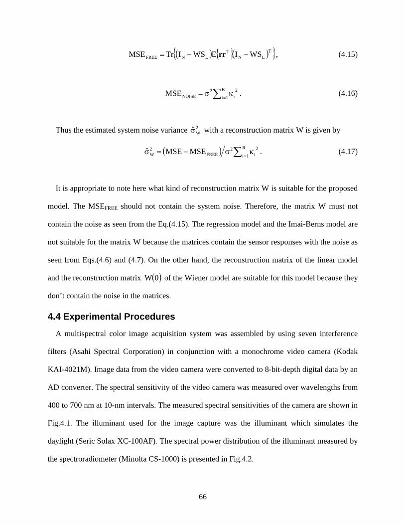
66

( ) { }( ){ }TLN

TLNFREE WSIEWSITrMSE −−= rr , (4.15)

∑ =κσ=

R

1i2

i2

NOISEMSE . (4.16)

Thus the estimated system noise variance 2Wσ with a reconstruction matrix W is given by

( ) ∑ =κσ−=σ

R

1i2

i2

FREE2W MSEMSEˆ . (4.17)

It is appropriate to note here what kind of reconstruction matrix W is suitable for the proposed

model. The MSEFREE should not contain the system noise. Therefore, the matrix W must not

contain the noise as seen from the Eq.(4.15). The regression model and the Imai-Berns model are

not suitable for the matrix W because the matrices contain the sensor responses with the noise as

seen from Eqs.(4.6) and (4.7). On the other hand, the reconstruction matrix of the linear model

and the reconstruction matrix ( )0W of the Wiener model are suitable for this model because they

don’t contain the noise in the matrices.




KAI-4021M). Image data from the video camera were converted to 8-bit-depth digital data by an

AD converter. The spectral sensitivity of the video camera was measured over wavelengths from

400 to 700 nm at 10-nm intervals. The measured spectral sensitivities of the camera are shown in

Fig.4.1. The illuminant used for the image capture was the illuminant which simulates the

daylight (Seric Solax XC-100AF). The spectral power distribution of the illuminant measured by

the spectroradiometer (Minolta CS-1000) is presented in Fig.4.2.

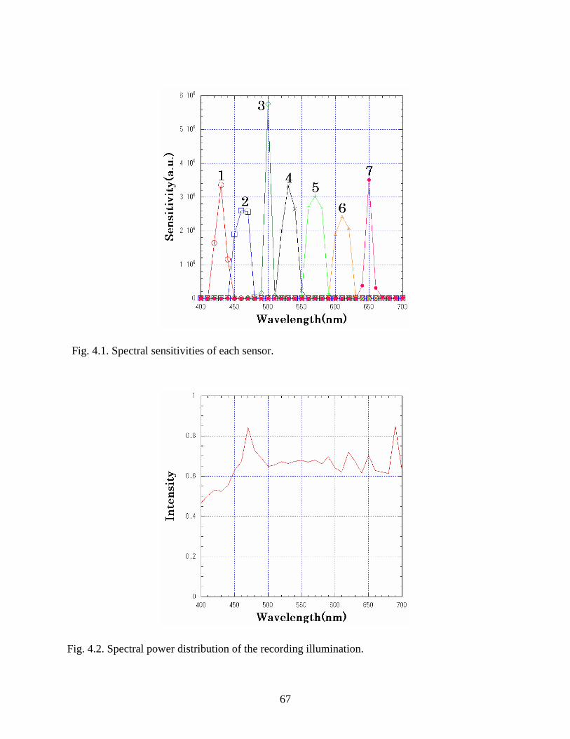
67

Fig. 4.1. Spectral sensitivities of each sensor.

Fig. 4.2. Spectral power distribution of the recording illumination.

68

The GretagMacbeth ColorChecker (24 colors) was illuminated from the direction of about 45

degree to the surface normal, and the images were captured by the camera from the normal

direction. The image data were corrected to uniform the nonuniformity in illumination and

sensitivities of the pixels of a CCD. The computed responses from a camera to a color by using

the measured spectral sensitivities of the sensors, the illuminant and the surface reflectance of the

color do not equal to the actual sensor responses since the absolute spectral sensitivities of a

camera depend on the camera gain. Therefore, the sensitivities were calibrated using an

achromatic color in the charts. In this work, the constraint was imposed on the signal power as

given by ( )TLSSL SRSTr=ρ , where relation of 1=ρ was used so that the estimated system noise

variance can be compared for different sensor sets. Various combinations of sensors from three

to seven in Fig.4.1 were used to simulate different sensor sets.

For the Wiener estimation developed in the previous model, the system noise variance was

estimated by the methods described above for each combination of sensors. Then the spectral

reflectances were recovered and the MSE of the recovered spectral reflectances was computed.

For other models, the spectral reflectances were recovered by each model and each MSE of the

recovered spectral reflectances was also computed.


In this chapter, the learning samples were the same as the test samples, i.e., the GretagMacbeth

ColorChecker was used for the test samples and the learning samples.

To estimate the influence of the system noise on the recovered spectral reflectances, a measure

for an increase in the MSE by the system noise is required. In the previous model which was

developed based on the Wiener estimation, the increase in the MSE ( WienerMSE∆ ) by the system

noise is denoted as

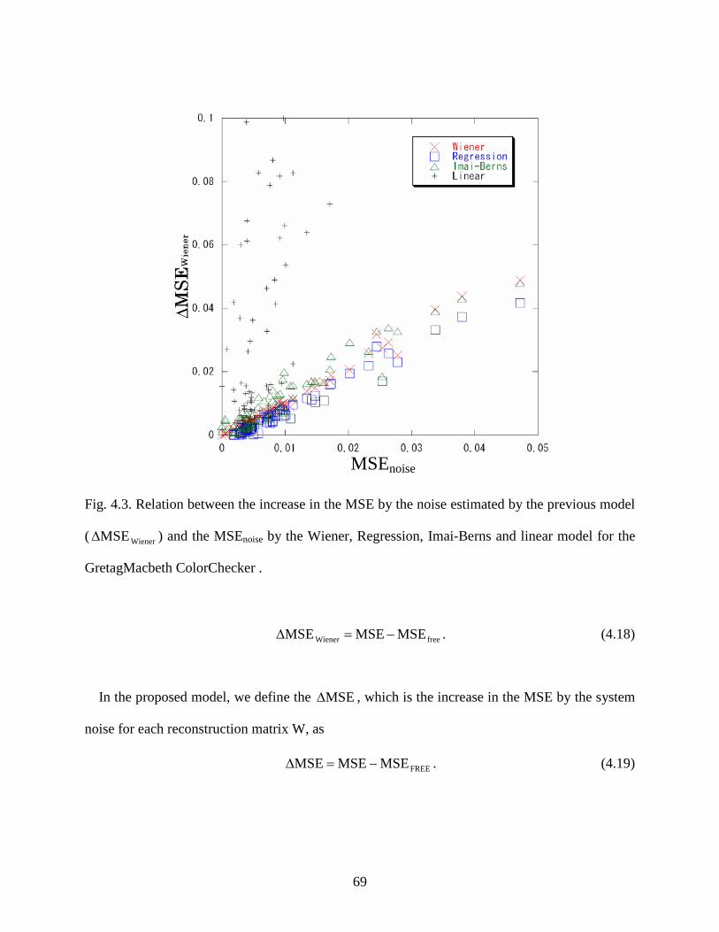
69

Fig. 4.3. Relation between the increase in the MSE by the noise estimated by the previous model

( WienerMSE∆ ) and the MSEnoise by the Wiener, Regression, Imai-Berns and linear model for the


freeWiener MSEMSEMSE −=∆ . (4.18)

In the proposed model, we define the MSE∆ , which is the increase in the MSE by the system

noise for each reconstruction matrix W, as

FREEMSEMSEMSE −=∆ . (4.19)

MSEnoise

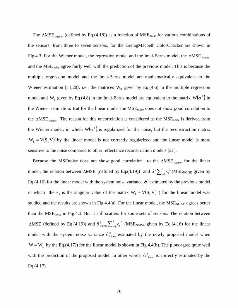
70

The WienerMSE∆ (defined by Eq.(4.18)) as a function of MSEnoise for various combinations of

the sensors, from three to seven sensors, for the GretagMacbeth ColorChecker are shown in

Fig.4.3. For the Wiener model, the regression model and the Imai-Berns model, the WienerMSE∆

and the MSEnoise agree fairly well with the prediction of the previous model. This is because the

multiple regression model and the Imai-Berns model are mathematically equivalent to the

Wiener estimation [11,20], i.e., the matrices RW given by Eq.(4.6) in the multiple regression

model and IW given by Eq.(4.8) in the Imai-Berns model are equivalent to the matrix ( )2W σ in

the Wiener estimation. But for the linear model the MSEnoise does not show good correlation to

the WienerMSE∆ . The reason for this uncorrelation is considered as the MSEnoise is derived from

the Wiener model, in which ( )2W σ is regularized for the noise, but the reconstruction matrix

( )+= VSVW LL by the linear model is not correctly regularized and the linear model is more

sensitive to the noise compared to other reflectance reconstruction models [21].

Because the MSEnoise does not show good correlation to the WienerMSE∆ for the linear

model, the relation between MSE∆ (defined by Eq.(4.19)) and ∑=κσ

R

1i2

i2ˆ (MSENOISE given by

Eq.(4.16) for the linear model with the system noise variance 2σ estimated by the previous model,

in which the iκ is the singular value of the matrix ( )+= VSVW LL ) for the linear model was

studied and the results are shown in Fig.4.4(a). For the linear model, the MSENOISE agrees better

than the MSEnoise in Fig.4.3. But it still scatters for some sets of sensors. The relation between

MSE∆ (defined by Eq.(4.19)) and ∑=κσ

R

1i2

i2Linearˆ (MSENOISE given by Eq.(4.16) for the linear

model with the system noise variance 2Linearσ estimated by the newly proposed model when

LWW = by the Eq.(4.17)) for the linear model is shown in Fig.4.4(b). The plots agree quite well

with the prediction of the proposed model. In other words, 2Linearσ is correctly estimated by the

Eq.(4.17).

71

Fig. 4.4. (a) Relation between the increase in the MSE ( MSE∆ ) by the linear model and the

MSENOISE ( ∑=κσ

R

1i2

i2ˆ ) with the noise variance estimated with the previous model for the


Fig. 4.4. (b) Relation between the increase in the MSE ( MSE∆ ) by the linear model and the

MSENOISE ( ∑=κσ

R

1i2

i2Wˆ ) with the noise variance estimated with the reconstruction matrix W for

the GretagMacbeth ColorChecker .

It is interesting to compare the estimated system noise variance of an image acquisition device

by the different models. Tbl.4.1 shows the optimum noise variance 2optσ that makes the MSE of

the Wiener estimation by Eq.(4.3) minimum, which was searched by the brute force method, the

estimated system noise variance 2σ by the previous model using Eq.(4.5) and the estimated

system noise variances 2Linearσ and 2

)0(Wσ by the proposed model using Eq.(4.17), where

LWW = for 2Linearσ and ( )0WW = for 2

)0(Wσ were used, respectively. The MSEs at each

estimated system noise variance, ( )2optMSE σ , ( )2ˆMSE σ , ( )2

LinearˆMSE σ , ( )2)0(WˆMSE σ , are also

∑ =R

1i2

i2 κσ ( )+

==∑ VSVWforκσ L

R1i

2i

2Linearˆ

(a) (b)

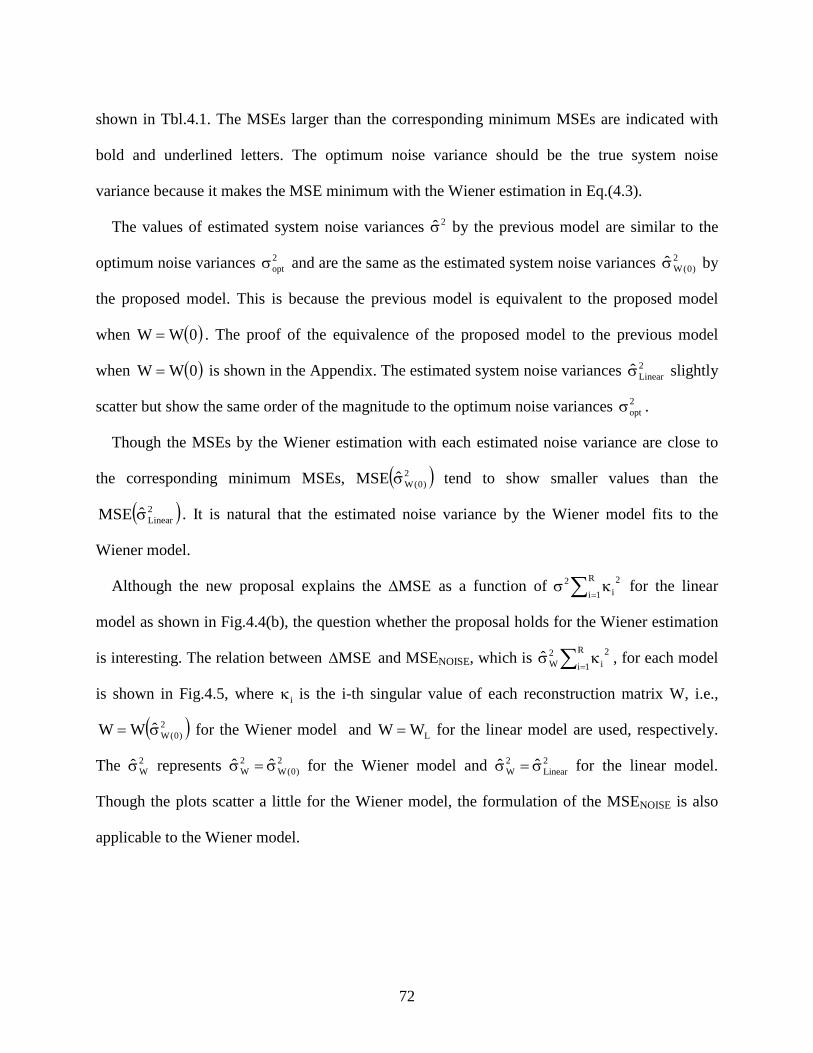
72

shown in Tbl.4.1. The MSEs larger than the corresponding minimum MSEs are indicated with

bold and underlined letters. The optimum noise variance should be the true system noise

variance because it makes the MSE minimum with the Wiener estimation in Eq.(4.3).

The values of estimated system noise variances 2σ by the previous model are similar to the

optimum noise variances 2optσ and are the same as the estimated system noise variances 2

)0(Wσ by

the proposed model. This is because the previous model is equivalent to the proposed model

when ( )0WW = . The proof of the equivalence of the proposed model to the previous model

when ( )0WW = is shown in the Appendix. The estimated system noise variances 2Linearσ slightly

scatter but show the same order of the magnitude to the optimum noise variances 2optσ .

Though the MSEs by the Wiener estimation with each estimated noise variance are close to

the corresponding minimum MSEs, ( )2)0(WˆMSE σ tend to show smaller values than the

( )2LinearˆMSE σ . It is natural that the estimated noise variance by the Wiener model fits to the

Wiener model.

Although the new proposal explains the MSE∆ as a function of ∑=κσ

R

1i2

i2 for the linear

model as shown in Fig.4.4(b), the question whether the proposal holds for the Wiener estimation

is interesting. The relation between MSE∆ and MSENOISE, which is ∑=κσ

R

1i2

i2Wˆ , for each model

is shown in Fig.4.5, where iκ is the i-th singular value of each reconstruction matrix W, i.e.,

( )2)0(WˆWW σ= for the Wiener model and LWW = for the linear model are used, respectively.

The 2Wσ represents 2

)0(W2W ˆˆ σ=σ for the Wiener model and 2

Linear2W ˆˆ σ=σ for the linear model.

Though the plots scatter a little for the Wiener model, the formulation of the MSENOISE is also

applicable to the Wiener model.

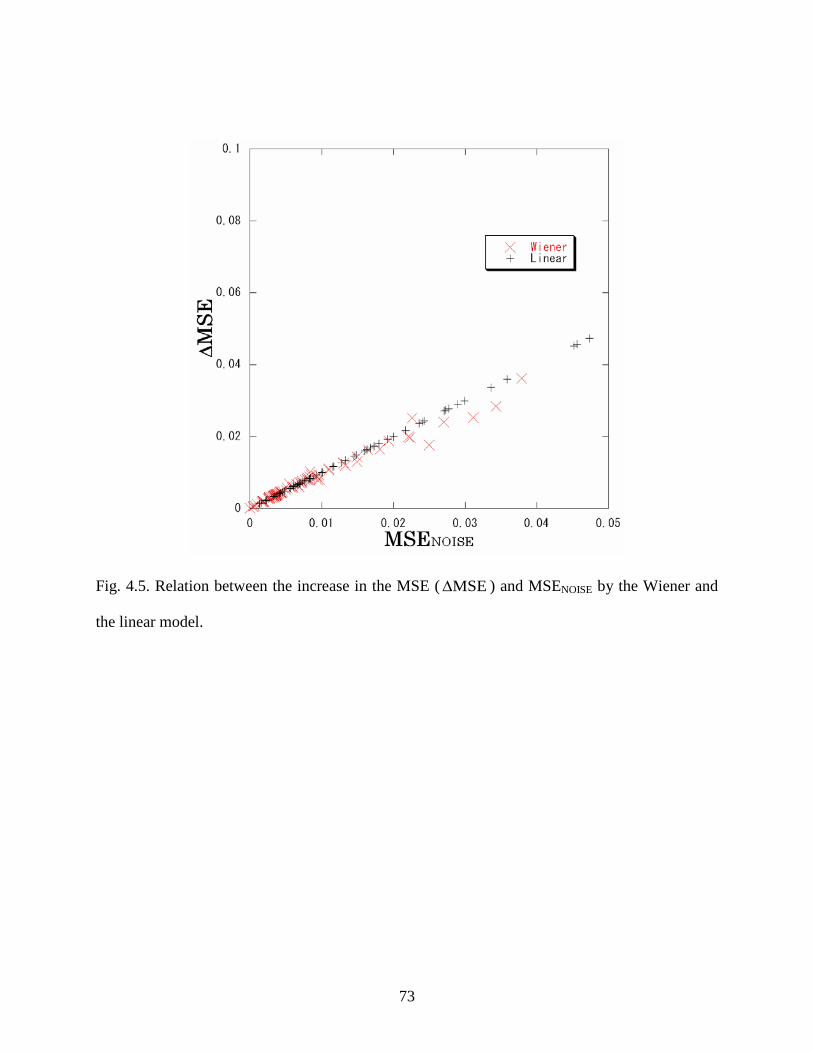
73

Fig. 4.5. Relation between the increase in the MSE ( MSE∆ ) and MSENOISE by the Wiener and

the linear model.

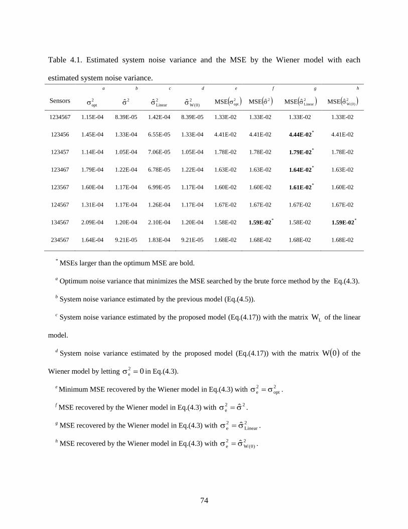
74

Table 4.1. Estimated system noise variance and the MSE by the Wiener model with each

estimated system noise variance. a b c d e f g h

Sensors 2optσ 2σ 2

Linearσ 2)0(Wσ ( )2

optMSE σ

( )2ˆMSE σ ( )2LinearˆMSE σ

( )2

)0(WˆMSE σ

1234567 1.15E-04 8.39E-05 1.42E-04 8.39E-05 1.33E-02 1.33E-02 1.33E-02 1.33E-02

123456 1.45E-04 1.33E-04 6.55E-05 1.33E-04 4.41E-02 4.41E-02 4.44E-02* 4.41E-02

123457 1.14E-04 1.05E-04 7.06E-05 1.05E-04 1.78E-02 1.78E-02 1.79E-02* 1.78E-02

123467 1.79E-04 1.22E-04 6.78E-05 1.22E-04 1.63E-02 1.63E-02 1.64E-02* 1.63E-02

123567 1.60E-04 1.17E-04 6.99E-05 1.17E-04 1.60E-02 1.60E-02 1.61E-02* 1.60E-02

124567 1.31E-04 1.17E-04 1.26E-04 1.17E-04 1.67E-02 1.67E-02 1.67E-02 1.67E-02

134567 2.09E-04 1.20E-04 2.10E-04 1.20E-04 1.58E-02 1.59E-02* 1.58E-02 1.59E-02*

234567 1.64E-04 9.21E-05 1.83E-04 9.21E-05 1.68E-02 1.68E-02 1.68E-02 1.68E-02

* MSEs larger than the optimum MSE are bold.

a Optimum noise variance that minimizes the MSE searched by the brute force method by the Eq.(4.3).

b System noise variance estimated by the previous model (Eq.(4.5)).

c System noise variance estimated by the proposed model (Eq.(4.17)) with the matrix LW of the linear

model.

d System noise variance estimated by the proposed model (Eq.(4.17)) with the matrix ( )0W of the

Wiener model by letting 02e =σ in Eq.(4.3).

e Minimum MSE recovered by the Wiener model in Eq.(4.3) with 2opt

2e σ=σ .

f MSE recovered by the Wiener model in Eq.(4.3) with 22e σ=σ .

g MSE recovered by the Wiener model in Eq.(4.3) with 2Linear

2e σ=σ .

h MSE recovered by the Wiener model in Eq.(4.3) with 2)0(W

2e σ=σ .

75

To examine the reason for the increase in the MSE by the system noise, the relation between

MSE∆ and ∑=κ

R

1i2

i or MSE∆ and 2Wσ by the Wiener and the linear model for various

combinations of the sensors is shown in Fig.4.6. The plots for the estimated system noise

variances lie in the nearly same order of the magnitude regardless of the increase in MSE∆ . It is

very important to note that the estimated noise variance does not contribute to the increase in

MSE∆ and that those estimates are nearly independent to the reconstruction models. On the

other hand, the values of ∑=κ

R

1i2

i increase with the increase in MSE∆ for the linear model,

whereas the values of ∑=κ

R

1i2

i remain almost constant for the Wiener model with the increase in

MSE∆ . This means that the increase in ∑=κ

R

1i2

i causes the increase in the MSE. In other words,

the system noise is amplified by ∑=κ

R

1i2

i as shown in Eq.(4.16) and this fact shows that the sum

of the squared singular values of the reconstruction matrix of the image acquisition device should

be small to design a noise robust system.

As mentioned above, the reconstruction matrices of the regression model and the Imai-Berns

models are not suitable for the proposed model because their reconstruction matrices contain the

system noise. Knowing this limitation, the relation between the increase in the MSE and the

MSENOISE are examined. For the regression model and the Imai-Berns model, MSEFREE gives

inaccurate values since the reconstruction matrices RW and IW contain the system noise, thus

another definition of the MSEFREE is required for the increase in the MSE.

Let the MSE with the sensor response p be )(MSEp p . Let rp SLˆ = then the MSE in the

noiseless case is denoted as )ˆ(MSEp p . Thus the pMSE∆ , the increase in the MSE by the system

noise, is defined without MSEFREE as

)ˆ(MSEp)(MSEpMSEp pp −=∆ . (4.20)

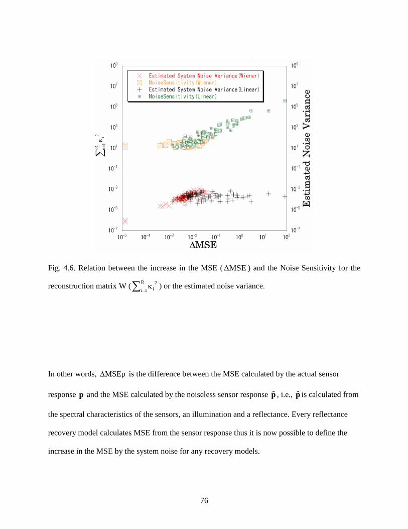
76

Fig. 4.6. Relation between the increase in the MSE ( MSE∆ ) and the Noise Sensitivity for the

reconstruction matrix W (∑=κ

R

1i2

i ) or the estimated noise variance.

In other words, pMSE∆ is the difference between the MSE calculated by the actual sensor

response p and the MSE calculated by the noiseless sensor response p , i.e., p is calculated from

the spectral characteristics of the sensors, an illumination and a reflectance. Every reflectance

recovery model calculates MSE from the sensor response thus it is now possible to define the

increase in the MSE by the system noise for any recovery models.

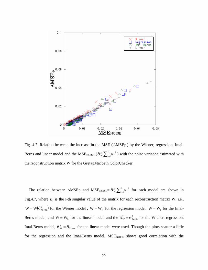
77

Fig. 4.7. Relation between the increase in the MSE ( pMSE∆ ) by the Wiener, regression, Imai-

Berns and linear model and the MSENOISE ( ∑=κσ

R

1i2

i2Wˆ ) with the noise variance estimated with

the reconstruction matrix W for the GretagMacbeth ColorChecker .

The relation between pMSE∆ and MSENOISE= ∑=κσ

R

1i2

i2Wˆ for each model are shown in

Fig.4.7, where iκ is the i-th singular value of the matrix for each reconstruction matrix W, i.e.,

( )2)0(WˆWW σ= for the Wiener model , RWW = for the regression model, IWW = for the Imai-

Berns model, and LWW = for the linear model, and the 2)0(W

2W ˆˆ σ=σ for the Wiener, regression,

Imai-Berns model, 2Linear

2W ˆˆ σ=σ for the linear model were used. Though the plots scatter a little

for the regression and the Imai-Berns model, MSENOISE shows good correlation with the

78

pMSE∆ for each model. The experimental results show that the proposal also holds for the

regression and the Imai-Berns models.

In addition to the above mentioned estimation of the noise variance by the Wiener and the

linear model, there is another method to formulate the reconstruction matrices W straight-

forward by the regression or the Imai-Berns model [22] and analyze the effect of the noise to the

image acquisition [23]. Further analysis to compare this straight-forward method with pMSE∆

is required to obtain more precise results.

4.6 Conclusions

A model for the influence of the noise on the accuracy of the recovered spectral reflectances is

proposed and is applied to the analysis of the increase in the MSE by the system noise for the

Wiener, regression, Imai-Berns and the linear model [24,25]. The experimental results by the

multispectral camera agree quite well with the proposed model. From this result, it is concluded

that the proposed model is appropriately formulated and that the separation of the MSE into

MSEFREE and the MSENOISE is essential to evaluate the influence of the system noise on the

image acquisition system. The proposed model also gives an advantage to estimate the system

noise variance for a reconstruction matrix W. The MSENOISE is expressed by the product of the

system noise variance and the sum of the squared singular values of the matrix W. The estimated

noise variances are almost independent to the matrix W and the sum of the squared singular

values is largely dependent on the matrix.

79

References 1. H. E. J. Neugebauer, "Quality Factor for Filters Whose Spectral Transmittances are Different

from Color Mixture Curves, and Its Application to Color Photography," J. Opt. Soc. Am. 46,

821-824 (1956) .

2. Poorvi L. Vora, H. Joel Trussell, "Measure of goodness of a set of color-scanning filters," J.

Opt. Soc. Am. A 10, 1499-1508 (1993).

3. G. Sharma, H. J. Trussell, “Figure of merit for color scanners,” IEEE Trans. Image Process. 6,

990-1001 (1997).

4. S. Quan, N. Ohta, R. S. Berns, and X. Jiang, “Unified measure of goodness and optimal

design of spectral sensitivity functions,” J. Imaging Sci. Technol. 46, 485–497 (2002).

5. N. Shimano, “Optimization of spectral sensitivities with Gaussian distribution functions for a

color image acquisition device in the presence of noise,” Opt. Eng. 45, 013201 (2006).

6. G. Sharma, H. J. Trussell, and M. J. Vrhel, “Optimal nonnegative color scanning filters,”

IEEE Trans. Image Process. 7, 129-133 (1998).

7. N. Shimano, “Recovery of spectral reflectances of objects being imaged without prior

knowledge,” IEEE Trans. Image Process. 15, 1848-1856 (2006).


image sensors,” Opt. Rev. 9, 81-88(2002).

9. N. Shimano, “Application of a colorimetric evaluation model to multispectral color image

acquisition systems,” J. Imaging Sci. Technol. 49, 588-593 (2005).

10. N. Shimano, “Evaluation of a multispectral image acquisition system aimed at reconstruction

of spectral reflectances,” Opt. Eng. 44, 107005 (2005).

11. M. Hironaga, N. Shimano, “Evaluating the quality of an image acquisition device aimed at

the reconstruction of spectral reflectances using recovery models,” J. Imaging Sci. Technol.

52, 030503 (2008).



13. N. Shimano, “Influence of Noise on Color Correction”, Proc. The first European Conference

on Colour in Graphics, Image and Vision, 549-553 (2002).

80

14. M. Hironaga, N. Shimano, “Influence of Noise on Estimating Spectral Reflectances”, Proc.

Color Forum Japan, 79-82 (2008).

15. Y. Zhao, L. A. Taplin, M. Nezamabadi and R. S. Berns, “Using the Matrix R Method for


(Granada, Spain), pp.469-472 (2005).

16. G. H. Golub, C. F. V. Loan, [Matrix Computations], The Johns Hopkins.

17. F. H. Imai, R. S. Berns, "Spectral Estimation Using Trichromatic Digital Cameras", Proc. Int.

Symposium on Multispectral Imaging and Color Reproduction for Digital Archives, Chiba,

Japan. 42-49, (1999).

18. L. Maloney, "Evaluation of linear models of surface spectral reflectance with small numbers

of parameters," J. Opt. Soc. Am. A 3, 1673-1683 (1986).

19. J. Parkkinen, J. Hallikainen, and T. Jaaskelainen, "Characteristic spectra of Munsell colors,"

J. Opt. Soc. Am. A 6, 318-322 (1989).

20. M. A. López-Álvarez, J. Hernández-Andrés and J. Romero, "Developing an optimum

computer-designed multispectral system comprising a monochrome CCD camera and a

liquid-crystal tunable filter," Appl. Opt. 47, 4381-4390 (2008).



22. M. Hironaga, N. Shimano and T. Toriu, "Estimating the Noise Variance in an Image

Acquisition System with Multiple Reconstruction Matrixes", ICIC Express Letters, Vol. 6,

No. 5, 1169-1174 (2012).

23. M. Hironaga, N. Shimano, T. Toriu, "Evaluating the Noise Variance of an Image Acquisition

System with Various Reconstruction Matrices", CGIV 2012,6th European Conference on

Colour in Graphics, Imaging 247-252, Amsterdam, the Netherlands (2012).

24. M. Hironaga, N. Shimano, "Estimating the noise influence on recovering reflectances", Proc.

SPIE, Vol.7529, 75290M, San Jose, California, USA (2010).



6148 (2010).

81

Appendix

Proof of the equivalence of the proposed model to the previous model where ( )0WW = .

As given by Eq.(4.13), the MSE of the recovered spectral reflectances by a matrix W is

expressed by

( ) { }( ){ } ( )WWTrWSIEWSITrMSE T2TLN

TLN σ+−−= rr . (A4.1)

The matrix ( )0W for the Wiener estimation with 02e =σ is represented by letting 02

e =σ in

Eq.(4.3) as

( ) ( ) 1TLL

TL RssSSRssS0W −

= . (A4.2)

Substitution of (A4.2) into (A4.1) leads the MSE at 02e =σ to

( ) ( ){ } ( )WWTrRssSRssSSRssSTr0MSE T2L

1TLL

TL

N

1i i σ+−λ=−

=∑ , (A4.3)

where the relations such as { } RssE T =rr , ( ) ∑ =λ=

N

1i iRssTr , and

( )( ) ( ){ }RssSRssSSRssSTrRssSRssSSRssSTr L1T

LLTLL

T1TLL

TL

−−=

were used to derive (A4.3).

SVD of 2/1LVS Λ in Eq.(A4.3) leads to the previous formula Eq.(4.5),i.e.,

( ) 2vj

2iji

R

1j

N

1i

22iji

R

1j

N

1ii

N

1i

bb0MSE

κ

λ∑∑σ+λ∑∑−λ∑======

. (A4.4)

On the other hand, in the new proposal, SVD of the matrix of (A4.2), ( )0W , is directly

performed. By combining Eqs.(4.14),(4.15) and (4.16), the MSE at 02e =σ , i.e., ( )0MSE is

expressed from (A4.1) as

( ) ( )( ) { } ( )( ){ } ∑ =κσ+−−=

R

1i2

i2T

LNT

LN S0WIES0WITr0MSE rr . (A4.5)

82

As seen Eqs.(A4.4) and (A4.5), ( )0MSE is expressed differently, depending only on the

difference of the SVD, and the ( )0MSE is divided into the noise independent first term and the

noise dependent second term. Therefore, these noise-independent terms and noise-dependent

terms are equivalent in Eqs. (A4.4) and (A4.5), respectively.. The estimate of 2σ gives the same

value since the both equations are derived from (A4.1).

The equivalence of the second term in Eqs.(A4.4) and (A4.5) gives the next relation.

∑ ∑∑ = ==κλ=κ

R

1j

N

1i

2vj

2iji

R

1j2

j b . (A4.6)

Therefore, the singular values in the previous model and the new proposal have the next relation.

∑=κλ=κ

N

1i

2vj

2iji

2j b . (A4.6)

As seen from the Eq.(4.4), if 2vjκ << 2σ then the MSENOISE becomes dominant, which means that

2jκ increases with the decrease in 2v

jκ .

83

Chapter 5

Overall Conclusions

In this chapter, the overall conclusions of the research for recovering the spectral

reflectances of objects being imaged by an image acquisition system are presented. The

proposed method and experiments done in each chapter of this thesis are summarized and

the future works are also discussed here.

84

To reproduce and recognize colors under the influence of the illuminants, the recovery of the

reflectances of the objects being imaged is required. The recovery is generally an inverse

problem and is largely affected by the noise in the image acquisition device. Because the Wiener

estimation is effective for solving inverse problems, accurate estimation of the noise variance in

the image acquisition system is required for accurate estimation of the reflectances by the Wiener

estimation. On the other hand, every image acquisition device has a different character; some

image acquisition devices are robust and insensitive to the noise while others are not robust and

sensitive to the noise. To design robust image acquisition devices to recover accurate

reflectances of objects and reproduce accurate colors, a method to evaluate the image acquisition

device is required.

This thesis addressed the following topics with experimental results and mathematical proofs.

In chapter 2, the spectral evaluation model based on the Wiener model proposed by Shimano was

applied to the regression and the Imai-Berns models and it was confirmed that the proposed

model can be applied to different models. In chapter 3, it was confirmed that the colorimetric

evaluation model based on the Wiener model proposed by Shimano can be applied to the

regression and the Imai-Berns models. And the noise robustness of the evaluation model was

examined and it was confirmed from the experimental results that the proposed model holds even

in a noisy condition. In chapter 4, the noise estimation model based on the Wiener estimation

proposed by Shimano was extended to a comprehensive model with a reconstruction matrix W

and the mean square errors (MSE) between the recovered spectral reflectances with various

reconstruction matrices W and actual spectral reflectances are divided into the noise independent

MSE (MSEFREE) and the noise dependent MSE (MSENOISE). It was shown that the relation

between the increase in the MSE and the MSENOISE agrees quite well in the experimental results

85

by the multispectral camera and that the estimated noise variances are in the same order of the

magnitude when the matrix W is of the Wiener model or of the linear model.

This thesis mainly addressed the influence of the noise to the image acquisition devices. For

more accurate recovery of the reflectances, the choice of the learning samples is important. We

tried to build a model to choose the appropriate learning sample for accurate recovery of the

reflectances and some experiments are done to confirm the model but further study is required to

improve the accuracy of the recovery. At the same time, an application to be used in business,

out of laboratory, in much noisier environment should be developed to show the usefulness and

trustworthiness of the proposed model.

86

Acknowledgements

First and foremost, I would like to express my indebtedness and deepest sense of gratitude to

my reverend supervisor and mentor Professor Takashi Toriu, Graduate School of Engineering,

Osaka City University, for his competent guidance, continuous encouragement, everlasting

understanding, and strong support on numerous occasions throughout the entire phase of my

research work.

I would like to express my immense sense of gratitude to the member of my thesis committee,

Professor Ikuo Oka, Graduate School of Engineering, Osaka City University, for his helpful

suggestions. His benevolent inspiration and kind observation motivated me to perform this novel

task.

I owe the immense measure of gratitude to the member of my thesis committee, Professor

Hideya Takahashi, Graduate School of Engineering, Osaka City University, for his generously

responsive suggestions help me to write this thesis nicely.

I wish to express my gratitude to Professor Noriyuki Shimano, Graduate School of Science

and Engineering, Kinki University, for his thoughtful suggestions and constructive discussions. I

have been honored to share his superlative experience in the field of the multispectral color

science.

Finally, I would like to express my special thanks to retired Professor Sadahiko Nagae, Kinki

University, and retired Professor Takuya Nishimura, Kinki University, for introducing me to a

rich and beautiful area of research and for sharing with me their incredibly broad knowledge.

87

List of Publications

Journal Papers



030503(2008).





6148 (2010).

4. M. Hironaga, N. Shimano and T. Toriu, "Estimating the Noise Variance in an Image

Acquisition System with Multiple Reconstruction Matrixes", ICIC Express Letters, Vol. 6,

No. 5, 1169-1174 (2012).



6. N. Shimano and M. Hironaga, "Recovery of spectral reflectances of imaged objects by the

use of features of spectral reflectances," J. Opt. Soc. Am. A 27, 251-258 (2010).

88

Refereed Conference Proceedings

1. M. Hironaga, K. Terai and N. Shimano, "A model to evaluate color image acquisition

systems aimed at the reconstruction of spectral reflectances", Proc. 9th Int. Symposium on

Multispectral Color Sci. and Appl., Taipei, ROC 23-28 (2007)

2. N. Shimano, M. Hironaga, "Analysis of Mean Square Errors of Spectral Reflectances

Recovered by Multispectral Cameras", Proc. of 15th Color Image Conference 147-150

Albuquerque, USA (2007)

3. M. Hironaga, N. Shimano, "Colorimetric Evaluation of a Set of Spectral Sensitivities", CGIV

2008, 4th European Conference on Colour in Graphics, Imaging, and MCS/08 602-607,

Terrassa, Spain (2008)

4. N. Shimano, M. Hironaga, "A new proposal for the accurate recovery of spectral reflectances

of imaged objects without prior knowledge", Proc. of Archiving 2008 pp. 155-158, IS&T,

Bern, Switzerland (2008)

5. N. Shimano, M. Hironaga, "Adaptive Recovery of Spectral Reflectances by the Regularized

Wiener Filter",11th Congress of the International Colour Association Sydney, Australia

(2009)

6. M. Hironaga, N. Shimano, "Estimating the noise influence on recovering reflectances", Proc.

SPIE, Vol.7529, 75290M, San Jose, California, USA (2010)

7. M. Hironaga, N. Shimano, T. Toriu, "Evaluating the Noise Variance of an Image Acquisition

System with Various Reconstruction Matrices", CGIV 2012,6th European Conference on

Colour in Graphics, Imaging 247-252, Amsterdam, the Netherlands (2012)

Documents

A Noise Analysis for Recovering Reflectances of the …dlisv03.media.osaka-cu.ac.jp/contents/osakacu/kiyo/111TD...In chapter 5, the overall discussions and conclusions are summarized