Embed Size (px)
Citation preview

2016
UNIVERSIDADE DE LISBOA
FACULDADE DE CIÊNCIAS
DEPARTAMENTO DE BIOLOGIA VEGETAL
A stochastic model of centriole assembly
Marco António Dias Louro
Mestrado em Bioinformática e Biologia Computacional
Especialização em Biologia Computacional
Dissertação orientada por:
Prof. Doutor Francisco Dionísio
Doutor Jorge Carneiro


O trabalho desenvolvido para esta dissertação foi efetuado no âmbito de uma colaboração entre os grupos chefiados pelo Dr. Jorge Carneiro e pela Dr.ª Mónica Bettencourt-Dias, no Instituto Gulbenkian de Ciência.


Acknowledgements
First of all, I would like to thank the people who supported me during my first incursion into science. To
my supervisor, Jorge Carneiro – I am deeply grateful for all the discussions and insights you provided
regarding my work. Thank you also for presenting me to the world of quantitative and mathematical
biology. To Mónica Bettencourt-Dias – thank you for presenting me to this project. Thank you so much
for all your support all throughout and for allowing me to participate in so many different scientific
activities. To my colleagues at both the QOB and CCR groups – thank you for all the help you gave me
and for sharing your experiences in scientific research. Finally, a big thanks to the IGC community who
received me so well. I would also like to thank Francisco Dionísio for all the attention and for being an
inspiration as a teacher.
Second, I would like to thank my friends and my family – thank you for your unconditional support
and all your care. You are the lighter side of things and the ones you always cheer me up after a long
day. I cannot thank you enough for having you in my life.
i

ii

Abstract
The control of centrosome numbers is essential to ensure cellular integrity and viability. This control
depends on the ability of the centrosomal structure, the centriole, to undergo duplication once and only
once per cell cycle. It is known that the master regulator of centriole biogenesis is the enzyme Plk4.
A mathematical model of Plk4 activity was used to conclude that there is a concentration threshold
which must be overcome in order to produce enough active molecules to induce centriole biogenesis.
This suggests a mechanism for regulating the onset of centriole duplication but it does not relate Plk4
concentration to centriole numbers nor explain how the system can account for fluctuations in its levels.
In this dissertation we sought to provide an explanation for the fidelity of the process of centriole du-
plication. Our hypothesis is that the formation of an incipient scaffolding structure, named the cartwheel,
is the critical step for controlling centriole numbers. The cartwheel core is composed of stacked Sas-6
rings, a protein whose function depends on Plk4. We postulated that if Sas-6 tends toward stacking on
top of the first cartwheel that arises, promoting its elongation, instead of forming a new one this could
prevent the formation of supernumerary structures and indirectly account for noise in Plk4 concentra-
tion. In its turn, since one cartwheel corresponds to a single centriole, this could explain how centriole
numbers are kept in check.
We developed stochastic models in order to address the efficiency of the stacking mechanism in
controlling cartwheel/centriole numbers. Our analysis shows that even relatively low stacking rates are
sufficient for reducing the rate at which the second cartwheel is formed. The average rate of cartwheel
elongation on the other hand is approximately constant. Moreover, the response of the system to higher
Sas-6 availability is not linear, suggesting there is a set of conditions in which cartwheel numbers remain
approximately the same but their length varies.
In order to test some of these predictions, it is necessary to measure cartwheel length. We pro-
posed that this could be done by using the aspect ratio distribution of randomly generated cartwheel
cross-sections. We conducted a power analysis and concluded that this method can distinguish between
cartwheels of different lengths. Moreover, the average aspect-ratio can be used as a cartwheel length
estimator, at least in a given range of values.
Our analysis suggests that the proposed stacking mechanism can allow the cell to control cartwheel
and presumably centriole numbers. The same mechanism also implies that cartwheel length is dis-
tributed. We suggested a method which can simplify the experimental procedure for measuring these
lengths.
Keywords: Centriole duplication; Cartwheel assembly; Stacking mechanism; Stochastic chemical
kinetics; Cartwheel length estimation
iii

iv

Resumo
O controlo do número de centrossomas é essencial para garantir a integridade e a viabilidade da célula.
Este controlo depende da capacidade que a estrutura principal do centrossoma, o centríolo, tem em sofrer
duplicação uma única vez por ciclo celular. Sabe-se que o regulador principal da biogénese de centríolos
é o enzima Plk4. Um modelo matemático da atividade de Plk4 foi usado para concluir que existe um
limiar de concentração que deve ser ultrapassado de modo a produzir moléculas ativas suficientes para
induzir a biogénese de centríolos. Isto sugere um mecanismo de regulação da iniciação do processo de
duplicação dos centríolos mas não relaciona a concentração de Plk4 com o número de centríolos nem
explicar como o sistema pode ter conta flutuações nos seus níveis.
Nesta dissertação procurámos providenciar uma explicação para a fidelidade do processo de dupli-
cação centriolar. A nossa hipótese é que a formação de uma estrutura de suporte incipiente, nomeada de
"cartwheel", é o passo crítico para controlar o número de centríolos. O cerne da "cartwheel" é composto
de anéis empilhados de Sas-6, uma proteína cuja função depende de Plk4. Postulámos que se o Sas-6
tender para o empilhamento sobre a primeira "cartwheel" que surja, promovendo o seu alongamento,
ao invés de formar uma nova, poderia impedir a formação de estruturas supernumerárias e ter em conta
ruído nos níveis de Plk4. Por sua vez, dado que uma "cartwheel" corresponde a um único centríolo, isto
poderia explicar como o número de centríolos é controlado.
Desenvolvemos modelos estocástico de modo a abordar a eficiência do mecanismo de empilhamento
no controlo de número de "cartwheels"/centríolos. A nossa análise revela que mesmo taxas de empil-
hamento relativamente baixas são suficientes para reduzir a taxa a que a segunda "cartwheel" é formada.
A taxa média de alongamento, por outro lado, é aproximadamente constante. Adicionalmente, a resposta
do sistema à maior disponibilidade de Sas-6 não é linear, o que sugere que há um conjunto de condições
nas quais os números de "cartwheels" se mantêm aproximadamente iguais mas o seu comprimento varia.
De forma a testar algumas destas previsões, é necessário medir o comprimento das "cartwheels".
Propusemos que isto pode ser feito utilizando a distribuição de "aspect ratios" de secções de "cartwheels"
geradas aleatoriamente. Efetuámos uma análise de potência e concluímos que este método pode ser uti-
lizado para distinguir entre "cartwheels" de tamanhos diferentes. Adicionalmente, o "aspect ratio" médio
pode ser usado como um estimador do comprimento de "cartwheels", pelo menos num determinado in-
tervalo de valores.
A nossa análise sugere que o mecanismo de empilhamento proposto pode permitir que a célula
controle o número de "cartwheels" e, presumivelmente, de centríolos. Este mecanismo também resulta
numa distribuição do comprimento das "cartwheels". Sugerimos um método que pode simplificar o
procedimento experimental para medir estes comprimentos.
Palavras-chave: Duplicação de centríolos; Montagem de "cartwheels"; Mecanismo de empilhamento;
Cinética química estocástica; Estimação do comprimento de "cartwheels"
v

vi

Resumo alargado
A regulação do número de centrossomas é fundamental para garantir a viabilidade de uma célula. O
centrossoma é um organelo cuja função é altamente conservada em várias linhagens de eucariotas, nas
quais atua como o principal centro organizador de microtúbulos. Desempenha um papel fulcral na orga-
nização do fuso mitótico e, consequentemente, no processo de divisão celular. Sabe-se que a ocorrência
de anomalias numéricas, nomeadamente o surgimento de centrossomas supranumerários, tem conse-
quências frequentemente nefastas para a célula e para o organismo, sendo a mais notável, a incidência
de cancro.
A regulação do número de centrossomas depende sobretudo da capacidade que sua estrutura prin-
cipal, o centríolo, tem em duplicar-se uma única vez por cada ciclo celular. O centríolo consiste numa
estrutura proteica em forma de barril, composta por nove tripletos de microtúbulos que apresentam uma
simetria radial característica. Os avanços recentes nas áreas da transcriptómica e proteómica permiti-
ram caracterizar o leque de componentes centriolares, incluindo aquele que é frequentemente entendido
como o regulador principal da biogénese de centríolos, o enzima Plk4.
Um artigo recentemente publicado descreveu o mecanismo de atividade do Plk4. A sua ativação
e marcação para degradação via proteossoma dependem de um mecanismo de fosforilação em trans.
Um modelo matemático baseado neste mecanismo foi utilizado para concluir que existe um limiar de
concentração da proteína, o qual deve ser ultrapassado de modo a produzir um número suficiente de
moléculas ativas de modo a viabilizar o processo de duplicação. Embora isto defina um regime de
condições em que a célula está ou não permissiva à biossíntese de centríolos, não relaciona um dado
número de centríolos à concentração de Plk4, especialmente no que diz respeito ao surgimento de uma
e apenas uma estrutura nova, nem como o sistema consegue responder a flutuações nas concentrações
de Plk4 e manter o número correto de centríolos.
Para os efeitos desta dissertação, procurámos explicar como é que a célula pode garantir a fidelidade
do processo de duplicação centriolar. A nossa hipótese assenta na formação de uma estrutura de suporte
ao centríolo, que se forma nos estágios iniciais do processo biogenético, denominada de "cartwheel". O
cerne desta estrutura é composto por dímeros de Sas-6, uma proteína cuja função depende da atividade
do Plk4. Estes dímeros organizam-se em conjuntos de nove, com forma aproximadamente anelar, que se
empilham uns sobre os outros. Existem evidências de que o tamanho destas pilhas é variável. Portanto,
postulámos que após a formação da primeira "cartwheel" existe uma competição entre o empilhamento
de moléculas de Sas-6 sobre a mesma, de forma a originar uma pilha de anéis, e a possibilidade de formar
uma "cartwheel" nova. Se o empilhamento for predominante em relação à produção de novas estruturas,
e sob o pressuposto de que existe uma correspondência de um para um entre "cartwheels" e centríolos, a
célula poderá ser capaz de garantir que o processo de duplicação ocorra uma única vez. Este mecanismo
também permite explicar como o ruído na concentração de Sas-6 e, indiretamente, Plk4, é neutralizado.
Por exemplo, na eventualidade da ocorrência de um pico de concentração nos níveis das proteínas, este
seria consumido pelo alongamento das pilhas mas não pela formação de “cartwheels”/centríolos novos.
De modo a poder responder se este mecanismo de empilhamento seria eficiente no controlo do
número de "cartwheels" e, consequentemente, de centríolos, definimos dois modelos estocásticos. O
vii

primeiro considera que a formação da "cartwheel" é o resultado final de uma cadeia linear de acontec-
imentos, ao passo que o segundo tem em conta dinâmicas de oligomerização e empilhamento de Sas-6
mais complexas. A análise do primeiro modelo revelou que não é necessário considerar uma taxa de
empilhamento relativamente elevada para impedir que uma dada molécula de Sas-6 entre na composição
de uma segunda "cartwheel". De facto, é a possibilidade de impedir a sua formação em cada um dos
passos intermédios que constitui o fator determinante na redução da taxa de produção de "cartwheels"
novas. Mesmo quando uma fonte constante de Sas-6 é adicionada, a taxa de formação de "cartwheels"
na presença de um mecanismo inibitório é menor em várias ordens de magnitude que na ausência desse
mesmo mecanismo.
No que diz respeito ao segundo modelo, obtivemos resultados semelhantes relativos ao mecanismo
de empilhamento. Demonstrámos que não é necessário uma taxa de empilhamento relativamente elevada
para inibir a formação de "cartwheels" supranumerárias. De facto, a nossa análise revelou que mesmo
quando a produção de Sas-6 é aumentada, o sistema não responde linearmente, originando um menor
número de estruturas individuais. Por outro lado, o alongamento das "cartwheels" procede de forma
aproximadamente linear, em média. É possível depreender destes resultados que um ligeiro aumento nas
concentrações de Plk4/Sas-6 se traduza em pilhas mais longas mas não num número significativamente
maior de "cartwheels". Também observámos que em condições propícias ao surgimento de "cartwheels"
supra+numerárias, se a sua síntese for assíncrona, isso traduz-se uma diferença média de comprimen-
tos entre as várias estruturas individuais; quanto mais cedo uma dada "cartwheel" é produzida, mais
rapidamente inicia o processo de empilhamento e mais longa se torna em relação às outras.
Para testar experimentalmente as previsões dos modelos, uma possibilidade seria através da ma-
nipulação da expressão de Plk4/Sas-6 e avaliação da sua influência no número e comprimento das
"cartwheels". De entre estas duas quantidades mensuráveis, obter experimentalmente a segunda ap-
resenta mais dificuldades do ponto de vista técnico. De modo a colmatar algumas destas dificuldades,
sugerimos um método que consiste em estimar o comprimento das "cartwheels" através da distribuição
de "aspect-ratios" de secções aleatórias da estrutura. Efectuámos uma análise de potência que demon-
strou que não só é possível distinguir duas distribuições de comprimentos diferentes, como também é
possível estimar o comprimento de uma dada população usando o "aspect-ratio" médio como estimador,
pelo menos numa determinada gama de valores.
A validade dos modelos aqui apresentados depende sobretudo de dois pressupostos-chave. Em
primeiro lugar, os modelos assumem que a formação da cartwheel" é o passo determinante para o con-
trolo do número de centríolos. Quanto a este pressuposto, podemos garantir pelo menos que a sua síntese
é a primeira incidência no processo biogenético de que um centríolo está a ser formado. Em segundo
lugar, assumimos que a "cartwheel" tem uma composição que assenta em anéis nónuplos de Sas-6, e que
estes anéis podem formar pilhas sem restrição de comprimento. Caso o fator limitante da formação de
"cartwheels" não seja a proteína Sas-6, os modelos podem ser ainda válidos se o fator limitante putativo
mantiver a mesma organização, ou seja, conjuntos de nove subunidades que se empilham. No que diz
respeito ao comprimento das pilhas, se existir um processo concorrente à formação de "cartwheels" que
limita o seu alongamento, este deverá ser tido em conta pelos modelos. Embora não existam evidências
claras para tal, é um aspeto que deverá ser abordado no futuro.
Os nossos resultados demonstram que do ponto de vista teórico o mecanismo proposto pode explicar
viii

como a célula consegue controlar o número de centríolos, mediante a extrapolação de que estes corre-
spondem ao número de cartwheels. Adicionalmente, a análise dos modelos sugere que a "cartwheel"
tem uma distribuição de comprimentos, algo que não é frequentemente abordado na literatura. No en-
tanto, existem algumas evidências que o comprimento da "cartwheel" pode ser relevante do ponto de
vista fisiológico. Por fim, sugerimos um método que poderá constituir uma abordagem mais simples ao
problema de medir o comprimento de uma estrutura sub-celular.
ix

x

Contents
1 Introduction 11.1 Motivation . . . . . . . . . . . . . . . . . . . . . . . . . . . . . . . . . . . . . . . . . . 1
1.2 The centriole biogenetic pathway . . . . . . . . . . . . . . . . . . . . . . . . . . . . . . 2
1.3 A mechanism for controlling centriole numbers . . . . . . . . . . . . . . . . . . . . . . 4
1.4 Implementing the hypothesis . . . . . . . . . . . . . . . . . . . . . . . . . . . . . . . . 5
2 Aims and objectives 9
3 Model definition and analysis 113.1 Qualitative formulation of the model . . . . . . . . . . . . . . . . . . . . . . . . . . . . 11
3.2 A linear model of a biosynthetic pathway . . . . . . . . . . . . . . . . . . . . . . . . . 12
3.3 Fate of a single molecule . . . . . . . . . . . . . . . . . . . . . . . . . . . . . . . . . . 13
3.4 Including a constant input of molecules . . . . . . . . . . . . . . . . . . . . . . . . . . 15
3.5 Modelling second-order oligomerization and stacking . . . . . . . . . . . . . . . . . . . 19
3.5.1 General model dynamics . . . . . . . . . . . . . . . . . . . . . . . . . . . . . . 21
3.5.2 Relation between individual cartwheel formation and elongation . . . . . . . . . 22
3.5.3 Parameter dependence of cartwheel formation and elongation . . . . . . . . . . 25
3.5.4 Molecular levels of the intermediates . . . . . . . . . . . . . . . . . . . . . . . 27
4 A method for estimating cartwheel length 31
5 Discussion 355.1 Model assumptions . . . . . . . . . . . . . . . . . . . . . . . . . . . . . . . . . . . . . 35
5.2 Approach on model analysis . . . . . . . . . . . . . . . . . . . . . . . . . . . . . . . . 37
5.3 Perspectives on centriole biogenesis . . . . . . . . . . . . . . . . . . . . . . . . . . . . 38
6 Concluding remarks 41
Bibliography 43
Appendices 47Methods . . . . . . . . . . . . . . . . . . . . . . . . . . . . . . . . . . . . . . . . . . . . . . 49
Glossary . . . . . . . . . . . . . . . . . . . . . . . . . . . . . . . . . . . . . . . . . . . . . . 51
xi

xii

List of Figures
1.1 Centrosome structure . . . . . . . . . . . . . . . . . . . . . . . . . . . . . . . . . . . . 2
1.2 The centriole assembly process in human cells . . . . . . . . . . . . . . . . . . . . . . . 3
1.3 Structure of the cartwheel . . . . . . . . . . . . . . . . . . . . . . . . . . . . . . . . . . 4
1.4 Example of a second-order reaction and corresponding Petri net . . . . . . . . . . . . . 6
3.1 Illustration of a model for cartwheel assembly . . . . . . . . . . . . . . . . . . . . . . . 12
3.2 Petri net representation of the linear sequence model for a single molecule . . . . . . . . 13
3.3 The probability of forming the end product decreases with the length of the sequence
and ks . . . . . . . . . . . . . . . . . . . . . . . . . . . . . . . . . . . . . . . . . . . . 15
3.4 Petri net representation of the reaction sequence scheme with input . . . . . . . . . . . . 16
3.5 The formation time of the end product is much longer in the presence of a diverting
mechanism . . . . . . . . . . . . . . . . . . . . . . . . . . . . . . . . . . . . . . . . . 18
3.6 Petri net representation of the model . . . . . . . . . . . . . . . . . . . . . . . . . . . . 20
3.7 Time-evolution of the second-order system . . . . . . . . . . . . . . . . . . . . . . . . . 22
3.8 Formation of successive cartwheels occurs at an increasingly slower rate . . . . . . . . . 23
3.9 The average and variance in the number of stacked rings in each cartwheel increases
with time . . . . . . . . . . . . . . . . . . . . . . . . . . . . . . . . . . . . . . . . . . 24
3.10 Stacking is determinant for inhibiting cartwheel formation . . . . . . . . . . . . . . . . 25
3.11 Cartwheel elongation depends on the input and the number of structures that form . . . . 27
3.12 The distribution of intermediates is associated with cartwheel formation . . . . . . . . . 29
4.1 Cylindrical contour of the cartwheel and possible cross-sections . . . . . . . . . . . . . 32
4.2 Example of a random cross-section obtained with the algorithm . . . . . . . . . . . . . . 32
4.3 Aspect ratio distributions and power analysis . . . . . . . . . . . . . . . . . . . . . . . 33
4.4 Average aspect ratio as a function of cartwheel size . . . . . . . . . . . . . . . . . . . . 34
xiii

xiv

Chapter 1
Introduction
1.1 Motivation
Controlling the number of certain subcellular structures is essential to ensure cellular integrity and vi-
ability of the organisms. An example of this is the case of the centrosome. The centrosome is the pri-
mary microtubule-organizing center in several groups of eukaryotes, such as animals and higher fungi
(Fig. 1.1). When mature it consists of two to four centrioles surrounded by a proteinaceous matrix called
the pericentriolar material (PCM); despite some variability in centrosomal structure, most functional as-
pects are retained among lineages [1]. The majority of centrosomal functions rely on the centriole.
The centriole is a barrel-like arrangement of microtubule triplets displaying a highly conserved ninefold
radial symmetry [2, 3]. It plays a crucial role during mitosis in the organization of the mitotic spin-
dle. Moreover, the ability of the centriole to duplicate once and only once during each round of cell
division is critical for allowing the daughter cells to inherit the correct number of centrioles [4]. The
de-regulation of this duplication process can originate supernumerary centrioles or prevent them from
duplicating, which in turn can result in several anomalies, such as chromosome missegration, the forma-
tion of a multipolar spindle or failure in undergoing mitosis altogether [5]. Numerical abnormalities of
the like, in which supernumerary centrioles and centrosomes arise, have been linked to multiple human
disorders, such as cancer [5, 6], microcephaly and dwarfism [6, 7].
This makes the centrosome and the centrioles a prime target for biomedical research. On the other
hand, as a fundamental biology question, unraveling the mechanisms which determine this property is
essential to understand centrosomal and centriolar physiology as well as the regulation of cell division.
Even though recent technological advances have allowed to characterize the centriolar proteome [2] and
interactome [8], the process remains poorly understood from a mechanistic point of view. Nonetheless,
despite the plethora of centriolar components, the biogenetic process appears to depend on certain key
elements, namely Plk4. Plk4 has been identified as the master regulator of centriole duplication; it has
been shown that depletion of the endogenous protein prevents centriole biogenesis to occur while its
overexpression is sufficient to induce the formation of supernumerary centrioles [9]. However, it is still
not yet clear how its concentration is related to centriole numbers.
The key regulators in centriole biogenesis, namely Plk4, are generally understood as occurring at low
levels in physiological conditions [10], suggesting they can be highly susceptible to fluctuations. There-
fore, in order for centriole duplication to maintain its robustness the system must be able to counteract
these fluctuations. From all these considerations, we were inclined to ask if there is a mechanism which
can ensure centriole duplication occurs once and only once while also accounting for the robustness to
noise in the concentration of its limiting factors.
In order to fully understand any biological process, quantitative studies are necessary. With the ad-
vent of molecular systems biology, mathematical models have been increasingly used to extract knowl-
1

Figure 1.1: Centrosome structure. The centrosome is the main microtubule-organizing center in several eukaryotic lineages.The figure depicts a centrosome prior to duplication. It is composed of two barrel-like structures called centrioles surrounded bya protein matrix, the pericentriolar material (PCM). The centrosome contains one mature (mother) centriole, which has distaland subdistal appendages, and an immature (daughter) centriole . Each of the centrioles is composed by nine microtubuletriplets (the indicated A-, B-, and C-tubules, which are fused together). Duplication unfolds in late G1/S with the formation ofa single procentriole in association with each of the pre-existing ones, yielding a total of four. This number is halved duringcell division, such that each daughter cell inherits two centrioles. The pre-mitotic daughter centriole completes its developmentinto a mother centriole through the acquistion of the distal and subdistal appendages, as well as a PCM cloud. The procentriolealso transitions to a daughter centriole, thus reconstituting the centrosome. This figure was adapted from Brito et al. [4]
edge of these data [11]. However, these are still scarce when it comes to centriole biology. A recent
paper used a model of Plk4 phosphorylation dynamics to conclude that there is a concentration threshold
below which there are not enough active molecules to efficiently initiate centriole biogenesis [9]. While
this could explain how the cell prevents centrioles from forming ad liber, it does not relate active Plk4
concentration to centriole numbers and hence cannot explain how the duplication process is so strictly
controlled. In addition to quantifying protein levels it is also important to describe the stoichiometry
of supra-molecular complexes for accurately characterizing protein-protein interactions. In the absence
of these data, mathematical models can still make use of whatever is available, provide quantitative
predictions on the behavior of the system and describe the molecular mechanisms at hand. Therefore,
modeling is a suitable approach for answering the main question of this dissertation.
1.2 The centriole biogenetic pathway
Centriole duplication is an extremely complex process showing evidence of tight spatial and temporal
regulation (Fig. 1.2). It starts in interphase with a "licensing" step which triggers the initiation of the
duplication process [4]. During this stage, Plk4 is concentrated at the centrosome. The role of Plk4 in
centriole biogenesis depends on its self-activation through trans-autophosphorylation [9]. This mecha-
nism also targets it for proteasomal degradation [9]. Asterless/Cep152 has been shown to recruit Plk4
to the centrosome in D. melanogaster [12], whereas in human cells this depends on the cooperation
of Cep192 and Cep152 [13]. Another protein, STIL, has also been suggested to transport both Plk4
and Sas-6 to the centrosome, a function which depends on Plk4-mediated phosphorylation [14]. At the
centrosome, Sas-6 acts as the core component of a structure named the cartwheel, which is synthesized
near orthogonally to the walls of the pre-existing centrioles [15]. The formation of the cartwheel is the
first physical evidence of the nascent procentriole and of its characteristic ninefold symmetry [4]. De-
2

Figure 1.2: The centriole assembly process in human cells. a) At the onset of centriole duplication, Plk4 localizes to theouter wall of the pre-existing centrioles; b) The accumulation of Sas-6 and Cep135 leads to cartwheel formation; c) Microtubulenucleation ensues as CPAP localizes to the centrosome and recruits γ-tubulin; microtubules are polymerized and elongated bythe addition of α- and β -tubulin; the microtubule triplets bind to the cartwheel and enclose it in the procentriolar lumen;d) Centrosome separation occurs in G2, an event which precedes centriole disengagement during mitosis; e) Formation of afully mature centrosome accompanied by compositional changes in its protein content; f) Transition from daughter to mothercentriole through the recuitment of PCM components and acquisition of the distal and subdistal appendages, after another roundof cell division. Centriole duplication and cell cycle stages are indicated at the top and bottom of the image. Key moleculesand structural units are represented. Proteins represented in black indicate spatial and temporal localization in the assemblypathway. Proteins represented in red indicate the moment when they are dislocated from the centrosome. Proteins representedin green and orange represent increasing or decreasing levels at the daughter centriole, respectively. Figure retrieved fromBrito et al. [4]
fects in cartwheel structure frequently lead to structural aberrations and hinder the duplication process
[16]. After cartwheel formation, CPAP, centrobin and γ-tubulin are recruited, an event which initiates
microtubule nucleation around the cartwheel[4]. The development of the procentriole progresses with
microtubule elongation and centriolar capping. In late-G2 phase, the pre-existing centrioles separate
and further disengage during mitosis. Segregation of the centrioles during cytokinesis ensures that each
daughter cell inherits a single pair of centrioles. During early G1, the procentriole transitions into a
daughter centriole. The final steps of maturation occur after another mitotic round is completed and in-
volve the formation of distal and subdistal appendages and PCM recruitment, completing the transition
to a fully developed mother centriole.
It has been reported that the concentration of some key centriolar components oscillates along the
cell cycle. For instance, it has been shown that Plk4 levels peak during mitosis [17], despite the onset
of centriole biogenesis taking place during interphase. Also, centrosomal levels of STIL and Sas-6
are coordinated and reach their maximum during interphase [14]. Being limiting factors in centriole
biogenesis, this suggests the process is temporally regulated. Moreover, it has been shown that the
procentriole can reform in S-phase after the centrosome is ablated [18]. It has been shown that Cdk-1 has
a role in negatively regulating Plk4 and STIL activity during mitosis, which suggests there is an interplay
between centriole assembly and the cell-cycle machinery [19]. Concerning spatial regulation, other than
3

some centriolar components being actively concentrated at the centrosome, as we have mentioned, the
PCM also seems to create an environment which favors microtubule polymerization [20]. Studies have
shown that disruption of the PCM affects centriolar stability and eventually leads to centriole loss [21].
All these factors indicate regulation occurs at the various stages in centriole biogenesis, with a multitude
of pathways probably acting in concert to guarantee proper centriolar and centrosomal function. Even
so, centriole assembly depends mostly on a set of evolutionary conserved proteins. For example, in C.
elegans they have been identified as ZYG-1, SAS-4, SAS-5, SPD-2 and SAS-6, where the first three
are homologs of Plk4, CPAP and STIL/Ana2, respectively while the latter is a homolog to Sas-6 [22].
Therefore, it is also possible that the control of centriole duplication may also depend on a few key
mechanisms, with the remaining players in the network acting to confer more robustness to the process.
1.3 A mechanism for controlling centriole numbers
The earliest physical sign that a centriole is being formed is cartwheel assembly. Its central hub con-
sists of nine Sas-6 homodimers in ring-like arrangement (Fig. 1.3). The outwardly projecting coiled-coil
domains of the dimers constitute the cartwheel spokes, which terminate in a distal structure called the
pinhead. The pinhead consists of another protein, Bld10/Cep135, and binds to the A-tubule of the micro-
tubule triplets. Other proteins have been suggested to cross-link the Sas-6 dimers, such as Ana2/SAS-5,
further stabilizing the cartwheel.
Figure 1.3: Structure of the cartwheel. a) 3D-model of the Trychonympha cartwheel emphasizing the core and spokes (lightblue), and the pinheads (dark blue); b) Longitudinal image of a centriole with the cartwheel appearing in the proximal regionof the lumen, at the bottom. Figure adapted from [16]
Sas-6 stability and localization have been shown to depend on Plk4. FBWX5 is a F-box protein and
a subunit of the SCF ubiquitin ligase complex which targets Sas-6 for degradation and is itself targeted
for degradation by Plk4-mediated phosphorylation [23]. Therefore, Plk4 acts in preventing Sas-6 degra-
dation. Regarding its localization, Plk4-dependent phosphorylation of STIL is required for shuttling
4

Sas-6 to the centrosome. When this is impaired, it can lead to failure in duplicating the centrioles [14].
Sas-6 dimerizes through interactions between its coiled-coils, and is also able to form higher-order
structures through its globular N-terminal domains [24]. It has been shown that Sas-6 homodimers can
arrange into cartwheel-like oligomers of varying size in vitro, although in vivo it occurs almost always
in a ninefold symmetrical fashion. Despite that, quantitative studies have identified homodimers as
the most abundant Sas-6 species in human cells [25]. Even when the protein is expressed at higher
than physiological levels, the predominant oligomers contain about two to three dimers [24]. These
results suggest that larger Sas-6 complexes are unstable. Indeed, experimentally measured dissociation
constants for the N-terminal interaction revealed the interaction to be relatively weak [24]. So, although
Sas-6 is a fundamental building block of the cartwheel, its assembly may depend on more than its self-
oligomerization properties [26]. For instance, it has been shown that oligomerization of both Sas-6 and
Ana2 is required for centriole assembly in Drosophila embryos, and that the two proteins cooperate
in cartwheel formation [27]. Nevertheless, the key insights here are that Sas-6 is a limiting factor of
centriole biogenesis and that it organizes itself in the cartwheel as a ninefold dimer ring.
Another feature of the cartwheel is that these ninefold Sas-6 rings arrange into multi-layered stacks.
How these stacks assemble is not known. Some have speculated that these rings are formed in the lumen
of the mother centriole and then transported to their typical position near the outer wall [26], though this
has not been shown. Another feature of the cartwheel is that it shows length variation across different
species, though only a few experimental measurements have been reported. An extreme example of this
is the Trichonympha cartwheel which occupies approximately 90% of the centriolar lumen [28]. Other
results in Chlamydomonas and Spermatozopsis have shown that cartwheel length varies along the cell
cycle [29, 30]. The results also show a considerable degree of variation within each cell cycle stage.
This suggests that there may be naturally occurring differences in cartwheel length within the same cell
type.
From a modeling perspective on the control centriole numbers, cartwheel assembly shows some
interesting properties: 1) it can be directly correlated to a single centriole; 2) its assembly depends
on the master regulator of centriole biogenesis, Plk4; 3) its center hub contains Sas-6 homodimers
that oligomerize into ring-like structures with a precise stoichiometry; 4) Sas-6 rings form stacks, the
length of which may be variable. We hypothesize that these stacks elongate through the stacking of
Sas-6 molecules on top of an existing cartwheel, eventually adding new rings to the structure. After
the first complete ring is formed and if the stacking process is prevalent comparing to the formation of
other individualized rings, then the cell can prevent the formation of supernumerary cartwheels. This
should also account for the robustness to fluctuations in Plk4/Sas-6 levels. It could also explain how
the cartwheel would arise as a stacked structure. This is the central hypothesis of this dissertation: the
existence of a stacking mechanism which inhibits cartwheel formation and promotes the elongation of a
pre-existing one by the successive addition of rings.
1.4 Implementing the hypothesis
The aforementioned hypothesis was addressed through modeling. Mathematical models have been used
historically in physics to explain natural phenomena. In biology, their use is widespread in ecology,
5

metabolism and epidemiology, and there are also classical examples in neurophysiology and evolution-
ary theory, as well as developmental biology and immunology [31, 32, 33, 34]. In the past few years,
they have been brought to light due to the need of integrating systemically the ever-increasing volume
of genomic and proteomic data into regulatory networks [35].
Chemically reacting systems have also been subjected to modeling. The traditional approach is
through the use of deterministic reaction-rate equations which follow from the law of mass action [36].
In the past century, a stochastic discrete approach stemming from collision theory has been put forward.
From a physical standpoint, it better reflects the fact that molecules are individual entities. In practice, it
predicts the behavior of a system more accurately when the number of molecules is small compared to
the continuous deterministic approach.
Chemically reacting systems can be modeled in this framework using a single chemical master
equation which describe the temporal evolution of the number of molecules for all the species considered
[35]. It is essentially a Markov model - the evolution of the system is independent from its history
and the waiting time for each transition (reaction) is exponentially distributed. While the chemical
master equation has been viewed as mathematically intractable, there are some cases in which it can be
analytically solved. For the remainder, simulation methods such as the Gillespie algorithm have been
developed [36]. The discrete stochastic framework is ideal for implementing cartwheel assembly as a
chemically reacting system as it allows for the counting of individual structures, the explicit description
of the hypothesized biochemical process and for the characterization of its driving forces.
In 1962, Carl Adam Petri provided a formalism called Petri nets which has been redeployed to for-
mally represent and analyze chemical/biochemical reaction systems [37]. Petri nets are equivalent to the
more conventional chemical equations but depict chemical species and reactions in a more graphically
intuitive way (Fig. 1.4). Software tools such as Snoopy [38] make use of this notation in combina-
tion with simulation methods and the display of molecular counts for each species to animate reaction
networks. This supplies a visual aide for understanding the behavior of a system, of which we took
advantage using the above mentioned tool.
Figure 1.4: Example of a second-order reaction and corresponding Petri net. The figure represents a reaction systemin which a molecule of A and a molecule of B react to produce a molecule of C. The circles (places) indicate the indicatedchemical species. The black dots (tokens) represent the molecules of each species. The square (transition) represents thereaction which takes as input a molecule of both A and B and yields a molecule of C, as indicated by the arrows (edges orarcs). Refer to Methods for Petri net notation and definitions
6

To the best of our knowledge, there are no other examples of mathematical models addressing cen-
triole duplication mechanistically. There are some reports of Markov models being used for describing
the evolution of centriole numbers in a population of proliferating cells [39, 40], but place their focus
on centriole duplication and inheritance as cellular-scale processes. Our hypothesis on the other hand,
focuses on a putative mechanism at the molecular level.
7

8

Chapter 2
Aims and objectives
The overarching theme of this dissertation is the control of centriole duplication. The first goal of this
dissertation was to propose a biological model capable of explaining how a centriole could undergo a
single round of duplication per cell cycle. For this we started by collecting knowledge on the centriolar
assembly pathway and its key molecular components. Then, we sought for the simplest explanation
which could explain: 1) how a single centriole is formed; 2) how the system can account for molecular
fluctuations in the centriolar components. As we have stated, our hypothesis is that the cartwheel is the
minimal structure that will give rise to a centriole and that the stacking of its building blocks on top of
an existing cartwheel should inhibit the formation of a second one. Under fluctuations in the levels of
the building blocks, this should result in the cartwheel having a length distribution.
The second goal of this dissertation was to develop stochastic models based on this hypothesis
and reflecting different levels of complexity. To analyze these models we combined analytical and
simulation methods in order to best address each situation and to gain a more complete understanding
of our proposal. In general terms, we set out to explore the conditions in which formation of the second
cartwheel can be inhibited and how cartwheel formation and elongation depend on the model parameters.
Third, we deemed that measuring cartwheel length posed the more technically challenging require-
ment for testing model predictions. So, we suggested an experiment for obtaining the aspect-ratio dis-
tribution of random cartwheel cross-sections and conducted a power analysis to test whether it would be
able to distinguish different length distributions and if it can be used as tool for estimating length.
In summary, we intended to propose a mechanism which should explain how the cell controls cen-
triole numbers, to make quantitative predictions with respect to that mechanism through the use of
mathematical models, and to propose a method for analyzing experiments designed to test some of these
predictions.
9

10
Chapter 3
Model definition and analysis
In this section we define and discuss stochastic models based on the aforementioned hypothesis for
centriole control. We begin by supplying a qualitative formulation of the model in which we describe
our assumptions from a biological standpoint. Next, we defined a model which represents cartwheel
assembly as a linear sequence of steps in all of which Sas-6 molecules can be diverted. This reflects
the principle behind the proposed stacking mechanism. This model allows for direct mathematical
analysis and permitted us to quantify cartwheel formation times with respect to the diverting mechanism.
Finally, we construct a more complex model which includes second-order oligomerization and stacking
dynamics. We proceeded to analyze it using numerical simulations. In this case, analysis of the model
enabled us to address elongation dynamics in addition to cartwheel formation. The results for both
models were compared appropriately.
3.1 Qualitative formulation of the model
In this section we provide a qualitative description of a model which allows for the control of centri-
ole numbers through cartwheel assembly. Our hypothesis depends on a number of assumptions: 1)
the cartwheel is the simplest individualized structure which can be correlated to a single centriole, and
the earliest in the assembly pathway; 2) the minimal structure which defines the cartwheel is a ring of
nine Sas-6 dimers, which act as the fundamental building blocks in the assembly process; 3) the in-
termediates in the assembly process are defined by the number of dimers they contain and are formed
through oligomerization of smaller structures; 4) intermediates can dissociate into any combination of
their components but the formation of a ninefold ring, i.e. a cartwheel, is irreversible; 5) there is a con-
stant production of dimers which depends on the limiting factors of centriole biogenesis, such as Plk4;
6) intermediates in the cartwheel assembly process can irreversibly stack on top of an existing cartwheel;
7) the stacking of intermediates occurs in such a way that it allows for cartwheel-bound ninefold rings
to form, at all times, i.e. there is a constraint to stacking relative to ring size but there are no steric con-
straints regarding the disposition of intermediates on top of the cartwheel; 8) the successive addition of
rings can continue indefinitely, thus elongating the cartwheel; 9) stacking only occurs on newly formed
cartwheels and not on the ones present at the mother centriole. Fig. 3.1 displays a schematic overview
of the model.
This can be interpreted as a competition between cartwheel formation and elongation-by-stacking
for a constant input of Sas-6 dimers. In other words, as soon as the first cartwheel is formed, the
intermediates are diverted towards stacking, which in turn should inhibit the formation of additional
separate structures. In quantitative terms, it should be noted that the constant net influx of molecules
determines that there is a continuous formation and elongation of cartwheels. The critical insight is that,
in these terms, stacking should considerably delay the formation of additional structures.
11

Figure 3.1: Illustration of a model for cartwheel assembly. The figure displays the chain of events leading to cartwheelformation or elongation. The Sas-6 dimer (C1) is the fundamental building block of the cartwheel. Structures containing upto eight of these dimers represent intermediates in the process of cartwheel formation (in light blue and denoted Ci, where irepresents the dimer content of the intermediate). These are formed by combining smaller oligomers and are considered to beable to dissociate into their constituents. A reaction yielding a structure containing nine dimers defines a complete ring (darkblue) and originates a cartwheel (Cr), which is also a readout for a single centriole. Intermediates can stack on top of this ring(dark blue ring overlapped with light blue intermediates) in a way which allows for a new ring to form; an intermediate of sizei stacked on top of a cartwheel is referred to as Ci
*. Once this originates a complete ring stacked on top of a cartwheel, theresulting stack is also referred to as Cr. The stacking process can continue indefinitely, further elongating the stacks.
3.2 A linear model of a biosynthetic pathway
The hypothesis underlying the model described in the previous section is that the stacking mechanism
will inhibit the formation of more than one cartwheel. A simple question which we can ask is if we take
a single dimer which was just produced, what is the probability that it will end up in a new cartwheel,
given that it can also be incorporated into a stack. We can also ask if the presence of a cartwheel can
slow down the time of formation of the next one if there is a constant input of these molecules.
Since we assumed that there are multiple possible combinations for a molecule of a given species,
which in turn determines there are several paths to cartwheel formation or to stacking, it is impossible
to obtain direct answers to these questions. So, let us suppose for now that cartwheel assembly can be
simplified to a linear sequence of first-order reactions.
We define Ci as the set of species representing the intermediates of cartwheel assembly, with i
representing the order of the species in the sequence and ranging from 1 to the final step r. This index
can be thought of as the dimer content of each species, in which case r would represent the size of
the ring; i.e. r “ 9. We consider that molecules in state Ci can be converted into the next step in the
sequence, Ci+1, through an irreversible reaction with rate constant kon. Let us also consider that Ci can
be irreversibly diverted from the sequence, with rate constant ks. This can be likened to the presence of
a single cartwheel stacking up intermediates, with the difference that in this case there are no geometric
constraints regarding the size of the intermediates. Production of the first species in the sequence C1
occurs at a constant rate σ . Finally, we let Cr denote the end product of the sequence, i.e. the cartwheel.
This model can represented by the following reaction system:
˚σÝÝÑ C1
CikonÝÝÑ Ci`1
CiksÝÝÑ ¨ , iă“ r´1
(3.1)
12

Figure 3.2: Petri net representation of the linear sequence model for a single molecule. The Petri net represents the casefor r “ 9. The nine places represent the Ci species, ordered in ascending order from left to right. The token represents thesingle starting C1 molecule. The transitions connecting two places in the sequence represent the linear set of reactions leadingto the formation of the end product. The transitions without an output arc represent the diversion reactions which prevent themolecule from reaching the final state. Refer to Methods for Petri net notation and definitions.
.
It should be noted that this system simplifies both the proposed oligomerization and stacking mecha-
nisms. In the first case, it does not consider the possibility of combining intermediates of different sizes,
neither their ability to dissociate. In the second case, it does not explicitly take into account the presence
of cartwheels in the sense that: 1) the stacking rate depends on the number of cartwheels; and 2) stack-
ing is not possible for all combinations of intermediates and cartwheel-bound species. For instance, a
cartwheel bound to a dimer triplet cannot capture an intermediate containing more than six dimers, as
that would exceed the size of a complete ring.
3.3 Fate of a single molecule
Consider a single molecule of the first species in the previously described sequence of intermediates. In
the presence of a diverting mechanism, it is faced with two possible final outcomes: it either reaches
the end of the sequence, thus forming a new structure, or it is diverted in its path. We can simplify the
reaction system described in (3.1) to:
CikonÝÝÑ Ci`1
CiksÝÝÑ C˚i , iă“ r´1
(3.2)
with kon representing the rate at which the initial C1 molecule progresses through each step of the
sequence, ks the rate at which is diverted and r is the length of the sequence. This is the simplest
representation of the mechanism we hypothesized regarding the control of cartwheel numbers.
An advantage of this system is that is amenable to mathematical analysis, which allows for the
derivation of general conclusions. We were interested in determining the probability that an initial C1
molecule is able to reach the final step of the sequence, Cr. Additionally we meant to quantify how
much this is reduced by increasing the value of diversion rate ks and the number of steps. This is akin to
asking how much the formation of a new cartwheel is inhibited by the stacking of Sas-6 intermediates
on a preexisting one and by the stoichiometry of the complete ring.
We begain by defining the random vector T“ pT1, ...,Tr´1qwhose elements are the residence time of
the molecule in the species Ci. These are assumed to be exponentially distributed with mean 1{pkon`ksq.
We proceed by defining a random vector O “ pO1, ...,Or´1q where each element Oi corresponds to the
sum of T1, ...,Ti. So, each Oi variable measures the random time it take to complete i reactions. By
13

definition, the probability distribution of the sum of random variables is the convolution of the cumu-
lative distribution function of each of the summed variables. Taking this into account, the cumulative
distribution function FOi variable can be defined recursively as:
FO1ptq “ FT1ptq
FO2ptq “ˆ t
0FT2pt´ τqFO1pτq dτ
...
FOiptq “ˆ t
0FTipt´ τqFOi´1pτq dτ
(3.3)
It should be noted that random times T or O do not distinguish if the initial molecule progressed
along the sequence of intermediates or if it was diverted. However, completing i reactions as the defini-
tion of O implies that the molecule did not get diverted in its path, for this event is irreversible. Therefore
we must condition the probability distribution functions on the probability that the intermediates remain
in the sequence after i reactions. It is also convenient to define the probability that the precursor was
modified up to the intermediate state Ci at a given time, which is expressed as:
PrpCi, tq “kon
i´1
pkon` ksqi FOi´1ptq´FOiptq (3.4)
PrpCr, tq “ˆ
kon
kon` ks
˙r
FOr´1ptq (3.5)
These expressions represent the probability that the reaction sequence reached the intermediate state
Ci (3.4) (or Cr in the case of (3.5)) and did not proceed at time t, conditioned on the probability that
there were no diversion events in none of the previous intermediate steps.
The fact that the precursor molecule C1 molecule can only undergo irreversible transformations
means that it will ultimately reach the final step or else be diverted somewhere along the sequence. So,
if one waits long enough the following asymptotic probabilities are reached:
limtÑ8
PrpCi, tq “ 0 (3.6)
limtÑ8
PrpCr, tq “ˆ
kon
kon` ks
˙r
(3.7)
where (3.7) is correctly understood as the maximal probability that the initial C1 molecule integrates
the final structure in this system.
This expression relating the two reaction rates and the number of reaction steps is the first theoretical
result of presented in this dissertation. The fraction`
kon{pkon` ks˘r represents the probability that a
given intermediate progressed towards the final step. Since each intermediate can be independently
diverted, the final probability is the product of the individual probabilities.
An increase in the diverting rate ks leads to a substantial decrease in the probability of reaching the
final structure (Fig. 3.3). For instance, a value of ks 5 times higher than that of kon is sufficient to prevent
more than 99% precursors to be integrated in the final structure, for all the indicated values of r. The
14

Figure 3.3: The probability of forming the end product decreases with the length of the sequence and ks. The curvesrepresent the expression in (3.7) as a function of ks for a sequence contain r number of steps. The probability of forming theend product decreases exponentially with the size of the sequence. The effect of ks is not as pronounced for relatively lowervalues. The value of kon was set to 1 for all cases. Note that the axes are in log-scale.
parameter r, the number of intermediate steps, is the parameter to which the probability of reaching
the final structure is more sensitive, decreasing exponentially with it. Applying this model to cartwheel
assembly and taking r“ 9, ks value need not even be higher than kon to reduce the probability of forming
more than one cartwheel, and consequently, by our assumption, more than one centriole. To give a more
practical example, it has been observed that approximately 98-99% of Drosophila testes cells contain
four centrioles in interphase [41]. Assuming that all of those cells successfully underwent centriole
duplication and that a cartwheel was also assembled for each centriole, a ks value of approximately 0.67
is sufficient to reproduce the results.
These quantitative considerations notwithstanding, the result of this simple probabilistic model can
only be interpreted as general trends of parameter dependence. The model is, by construction, limited
and oversimplified. For example, it is limited in the sense that it tells us nothing on the effect of a con-
tinuous source of the Sas6 dimers, as it is expected from a single-molecule analysis. It is oversimplified
because the reaction steps in the assembly of a ninefold cartwheel ring are not necessarily first-order or
sequential since Sas6 dimers and different intermediates can combine to form higher-order oligomers,
possibly the complete ring, in a single step.
3.4 Including a constant input of molecules
In the previous section we followed the fate of a single individual building block which can form a
final product after a number of sequential transformations. We now ask how the time in which the final
product forms changes in the presence (ks ą 0) or absence (ks “ 0) of a diverting mechanism, given that
there is a constant influx of molecules. To model this scenario, we retake the reaction system defined
in (3.1) and shown in Fig. 3.4).
The purpose here is to compare cartwheel formation times in the presence or absence of a pre-
existing cartwheel (diversion enabled vs. diversion disabled, respectively). While it still does not include
the more complex oligomerization possibilities mentioned above and corresponding constraints on the
15

stacking dynamics, the critical aspect is the addition of a continuous influx of molecules.
This reaction system consists exclusively of zero-order or monomolecular reactions, which are a
particular case of first-order reactions involving a single reactant and a single product. The increased
complexity of this system determines that the simple probabilistic model defined before cannot be ap-
plied. Normally, the model used for representing the situation at hand, and more broadly any chemical
reaction system, is the chemical master equation. The chemical master equation describes the temporal
rate of change in the probability of the system reaching in a given state, depending on its current one.
Generally its solution can only be approximated using numerical methods. However in this case, Jahnke
and Huisinga [35] provided a general solution which can applied to obtain the desired quantities.
Figure 3.4: Petri net representation of the reaction sequence scheme with input. Representation for r “ 9. The left-mosttransition represents a reaction which produces molecules of the first species in the sequence. The places and reactions are thesame as in Fig. 3.2.
So, first we define a random vector X“`
X1, ...,Xr´1˘ᵀPNr´1 whose elements represent the molec-
ular numbers of each Ci species. Note that the vector does not include the final species in the sequence,
Cr. This is important for achieving the final solution because in this way the formation of the end product
constitutes an exit from the system, in the same way as the diverting reactions, such that coupled with
the molecular influx this can be considered as an open system.
We now define
A“
¨
˚
˚
˚
˚
˚
˚
˚
˝
X1 X2 ... Xr´2 Xr´1
X1 ´pkon` ksq 0 ... 0 0
X2 kon ´pkon` ksq ... 0 0
... ... ... ... ... ...
Xr´2 0 0 ... ´pkon` ksq 0
Xr´1 0 0 ... kon ´pkon` ksq
˛
‹
‹
‹
‹
‹
‹
‹
‚
(3.8)
b“´
X1 X2 ... Xr´2 Xr´1
σ 0 ... 0 0¯
(3.9)
where A is a transition rate matrix and b is an input vector. Note that the entries of A are the rate
constants for the reactions originating a molecule of the species in row i from a molecule of the species
in column j. This is unconventional but necessary to allow some algebraic operations.
The steady-state distribution of X will be:
limtÑ8
Prpx, tq “P`
x,λ ptq˘
(3.10)
16

where P denotes the product (or multiple) Poisson distribution with expected value λ given by:
limtÑ8
9λ ptq “ A´1bᵀ (3.11)
with A and b defined in (3.8) and (3.9), respectively. The product Poisson distribution is the joint
distribution of a number of independent Poisson distributions, which in this case refer to the distribution
of each of Xi variables, with the parameter vector λ representing the steady-state expected value and
variance of each group of molecules. After substituting for A and b, we have:
λ “
ˆ
σ
kon` ks,
σkon
pkon` ksq2 , ...,
σkonr´2
pkon` ksqr´1
˙
(3.12)
.
On a side note, this solution is valid for any initial distribution of Ci molecules. We are interested in
knowing the time scales of formation of the end product in the sequence given that the molecules may
or may not be diverted and what is the response to molecular influx. However, the solution presented
in (3.10) does not include the outcome of the end product. As this system is first-order for all reactions
and Cr corresponds to a dead state, we know the average number of Cr molecules will grow linearly with
time. Also note that the formation of Cr depends exclusively on the penultimate intermediate state in the
sequence, Cr-1. Therefore, to formulate the rate of Cr formation, we weigh the expected value of Cr-1 by
the corresponding reaction rate constant, kon, take the time derivative and invert the result, such that the
expected time, and variance, of Cr formation θ is given by
θ “
„
σ
´ kon
kon` ks
¯r´1
(3.13)
This is the second theoretical result of this dissertation and is equivalent in practical terms to the
solution provided in (3.7). As it can be seen in figure 3.5, θ decreases linearly when only the molecular
influx in allowed to vary. The variance of θ follows the same trend. Comparing the two lines, when
diversion is allowed by setting ks to a value of 1, it is sufficient to produce a 100-fold increase in θ . This
result suggests that even under a constant influx of molecules, the nine independent steps in which the
molecule can be diverted are sufficient to produce a substantial increase in the average time of formation
of the end product. When diversion is enabled, θ eventually reaches an asymptote for increasing kon.
The value of the asymptote corresponds to the value of θ when the diversion mechanism is disabled.
The growth of θ as a function of ks is symmetrical to that of kon; the average formation time of the end
product increases rapidly for higher ks but is not very sensitive to lower values. Note that formation of
the end product when ks “ 0 is independent of kon in the considered range of values. It can be observed
in (3.13) that this is true for any positive value of kon. So, in these conditions, the maximum speed at
which the end product is formed is limited only by the input parameter.
It should be noted that steady-state expected value of the time of end product formation is equal to
the result obtained in (3.7) weighed by σ . Therefore, it can be stated that the average behavior of a group
of molecules is simply a product of individual behaviors. This also suggests that both theoretical results
are consistent with one another.
17

Figure 3.5: The formation time of the end product is much longer in the presence of a diverting mechanism. The twocurves represent situations in which diversion from the main reaction sequence is either enabled (ks ą 0) or disabled (ks “ 0).θ decreases linearly with σ but is 100-fold higher when diversion is enabled. This shows that diversion can significantly delaythe formation time of the end product. The growth of θ as a function of kon and ks is symmetrical; it converges to a minimumvalue as kon increases and is not very sensitive to ks for relatively low values. All parameter values other than the one indicatedwere set to 1 and we are considering r “ 9. The curve for ks “ 0 is kept in the third plot for reference purposes.
18

3.5 Modelling second-order oligomerization and stacking
In the previous section we analyzed a simplified linear model of cartwheel assembly. In this section we
will include second-order kinetics to better reflect the formation of Sas-6 intermediates and cartwheels
through oligomerization. We will also represent stacking explicitly taking into account the presence of
the cartwheel and the stoichiometric bounds we postulated on stacked ring formation.
We reuse the Ci notation to represent intermediates composed of i Sas-6 dimers. Influx of single
dimers (C1) occurs at a constant rate σ . Ci species oligomerize with rate constant kon. The product of
these reactions should yield a molecule no larger than nine-dimers, which constitutes the complete ring,
or the minimal structure which defines an individualized cartwheel. Dissociation of the intermediates
into any combination of their constituents occurs with rate constant koff . The reaction which leads to
the formation of a complete ring is considered to be irreversible. Stacking of the intermediates on top
of a cartwheel occurs with rate constant ks and is considered to be irreversible as well. This process
should be interpreted as ring formation on top of an existing cartwheel, eventually yielding a stack of
rings. All cartwheels whose top-most layer is a complete ring will be denoted by Cr whereas others
where it is incomplete will be represented by Ci*, with i indicating the number of dimers in the top-most
layer. In practical terms, when an intermediate stacking on a Ci* molecule would produce a new ring, it
is modeled as returning to Cr. We are assuming that there are no steric constraints associated to stacking.
For example, if a dimer (C1) would stack on top of a cartwheel already bound to another dimer (C1*), they
would form the equivalent to a cartwheel bound to a C2 molecule (C2*). This model can be represented
by the following reaction system (Fig. 3.6):
˚σÝÝÑ C1
Ci`CjkonÝÝáâÝÝ
koffCi`j, i` j ă r
Ci`CjkonÝÝÑ Cr, i` j “ r
C˚i `CjksÝÝÑ C˚i`j, i` j ă r
C˚i `CjksÝÝÑ Cr, i` j “ r
(3.14)
where the first line represents constant influx of Sas-6 dimers into the system; the second line
represents oligomerization reactions; the third line represents the formation of a complete ring, i.e.
a cartwheel; the fourth line represents the irreversible stacking of oligomers on top of an existing
cartwheel; and the fifth line represents the formation of a complete ring on top of a cartwheel. Here, i
and j represent the dimer content of a given intermediate and r is ring size.
When converted to a mathematical model, this reaction system features two relevant outputs: the
number of cartwheels which have formed and the number of stacked rings in those cartwheels, or stack
length, in a given time. Regarding the second, it should be stated using Cr and Ci* is an abuse of notation
and prevents us from measuring stack length directly. However, one can easily circumvent this issue by
counting the number of times a Ci* is reconverted into Cr. In this way, one can avoid having to deal with
an indeterminate number of chemical species, which is highly convenient since the simulation tool we
used is limited in that respect. Since the length of the stacks has no implications for the dynamics of the
19

Figure 3.6: Petri net representation of the model. The upper sequence of places (red box) depicts all the Ci species, inascending order of dimer content and the lower line is the equivalent for the C*
i species (orange box). The rightmost places,at halfway between both lines, represent cartwheels, i.e. complete rings or stacks, (top) and a counter for the total number ofstacked rings (bottom). Above the upper line of places are the transitions corresponding to reversible Sas-6 oligomerization.The corresponding set below the lower sequence of places represent the stacking reactions. The leftmost transition, with noinput arc, represents dimer production.
20

model, this abuse of notation is not problematic.
It should be noted that we are making some simplifications regarding the chemical reactions, namely
when it comes to ring formation and stacking. In the first case, the formation of a complete ring requires
the formation of two chemical bonds in order to circularize the structure. In the second case, stacking
implies that the incoming intermediate interacts with the cartwheel as well as with any other molecule
already bound to its top ring.
3.5.1 General model dynamics
Having established this, the main questions we can ask to the model is if cartwheel formation can be
inhibited in such a way that one and only one structure is formed, and how this depends on stacking.
Rephrasing this as a kinetic issue, can the second event of cartwheel formation take much longer, on
average, than the first? Moreover, what is the relation of cartwheel number with the length of the stacks?
Unlike in the previous model, this one is not easily tractable so we proceeded to analyze it with using
numeric simulations. As a starting point, we considered a condition in which all the parameters were
set to a value of 1, heretofore referred as the reference condition. We also considered another condition
in which σ was set to 5 to test whether cartwheel formation could still be comparatively inhibited
even with higher influx. This will be referred to as the high influx condition. We implemented the
model in Snoopy and performed 1000 independent simulations with the Gillespie algorithm from an
initial condition where no molecules were present and extracted the average number of cartwheels and
intermediates at discrete time points, as well as the length of the stacks (Fig. 3.7). The stopping condition
for the simulations was t “ 100.
The results presented in Fig. 3.7 A show the time evolution in the average number of cartwheels (i.e.
all Ci* species as well as Cr and intermediates. Due to the initial absence of intermediates there is a delay
in cartwheel formation as dimers are being produced and oligomerized into higher-order structures.
In the reference condition, the average number of cartwheels rises and causes a drop in the levels of
the intermediates as they begin to be diverted towards stacking. After one cartwheel has formed, new
ones appear at a much slower rate. In the high influx condition, approximately 2.5 cartwheels form on
average in the considered time window but the decrease in their rate of formation and the levels of the
intermediates is still visible. These results suggest that in the given time window, it is not necessary to
increase the stacking rate in order to ensure the formation of a single cartwheel. Even when the molecular
influx is increased five-fold, there is not a linear response in the average number of cartwheels compared
to the reference condition. This also corroborates our previous findings that if a large number of steps are
required to give rise to a final product, the presence of a diverting mechanism at each step is sufficient
to reduce the probability of reaching that outcome. In other words, the ninefold stoichiometry of the
cartwheel can determine that a relatively higher stacking rate may not be needed to inhibit formation of
new structures.
Regarding the length of the stacks, it can be observed in Fig. 3.7 B that the number of stacked
rings eventually becomes a linear function of time. The slower elongation rate in the initial moments
of the simulations is due to the fact that few cartwheel have formed by then. Comparing the two condi-
tions, when σ is set to a value of 5 the rate of elongation is faster but the response is again non-linear.
21

Figure 3.7: Time-evolution of the second-order system. A – Model dynamics reveal that cartwheel formation is eventuallyinhibited. The curves represent the temporal change in the average number of molecules from 1000 simulations. Cartwheelsstart being produced after a certain time leading to a decrease in the numbers of the intermediates. For σ “ 1 (referencecondition) the average cartwheel formation rate slows down after the first one has formed. For σ “ 5 (high influx condition) itslows down after forming two cartwheels on average but less intensely than in the reference condition. B – Average cartwheellength is approximately linear. The curves represent the temporal evolution of stack length averaged over cartwheel numbersand simulations. Elongation accelerates as cartwheels are being formed and eventually reaches a steady rate. Time (t) is inarbitrary units.
This suggests that the production is the limiting factor for the length of the stacks, such that the pool of
molecules is divided between all the existing cartwheels. Also, we can conclude that after a certain num-
ber of cartwheels have formed, assembly of new structures is very rare and the stacks keep elongating.
In the reference condition, this occurs after one has formed on average.
3.5.2 Relation between individual cartwheel formation and elongation
These results are informative regarding the inhibition of cartwheel synthesis. However, since we are
interested in cartwheel numbers it is important to look into the times of each individual cartwheel for-
mation event. The cumulative distribution of the times at which a new cartwheel is formed in each
individual simulations is shown in Fig. 3.8.
In the reference condition the first cartwheel forms relatively quickly in all simulations. The second
cartwheel on the other hand only forms in 0.15% of the simulations in the considered time window. In
the high influx scenario, both the first and second cartwheels form on all simulations, albeit the sec-
ond appearing at a slower rate, and the third is able to form in approximately half of the simulations.
The main observation is that both the average time and variance increase for successive cartwheel for-
mation events, such that the overlap between the distributions of each individual event is reduced. A
consequence of this is that the diversity of cartwheel numbers at a specific time point is small, as it
can be seen in the histograms. These results suggest that the model cannot only explain how cartwheel
formation is inhibited but also that there is a certain degree of robustness in forming a certain number
of cartwheels. The reference condition satisfies the answer to the main question regarding cartwheel
numbers in the sense that one is formed for sure and the occurrence of the second one is a very rare and
unlikely event in the considered time interval.
In the same way as we have asked what are the dynamics of each individual formation events, we
should also ask how each individual cartwheel elongates. For that, we looked into stack length for the
two situations we have studied up to this point. The implementation of the model did not allow us to
22
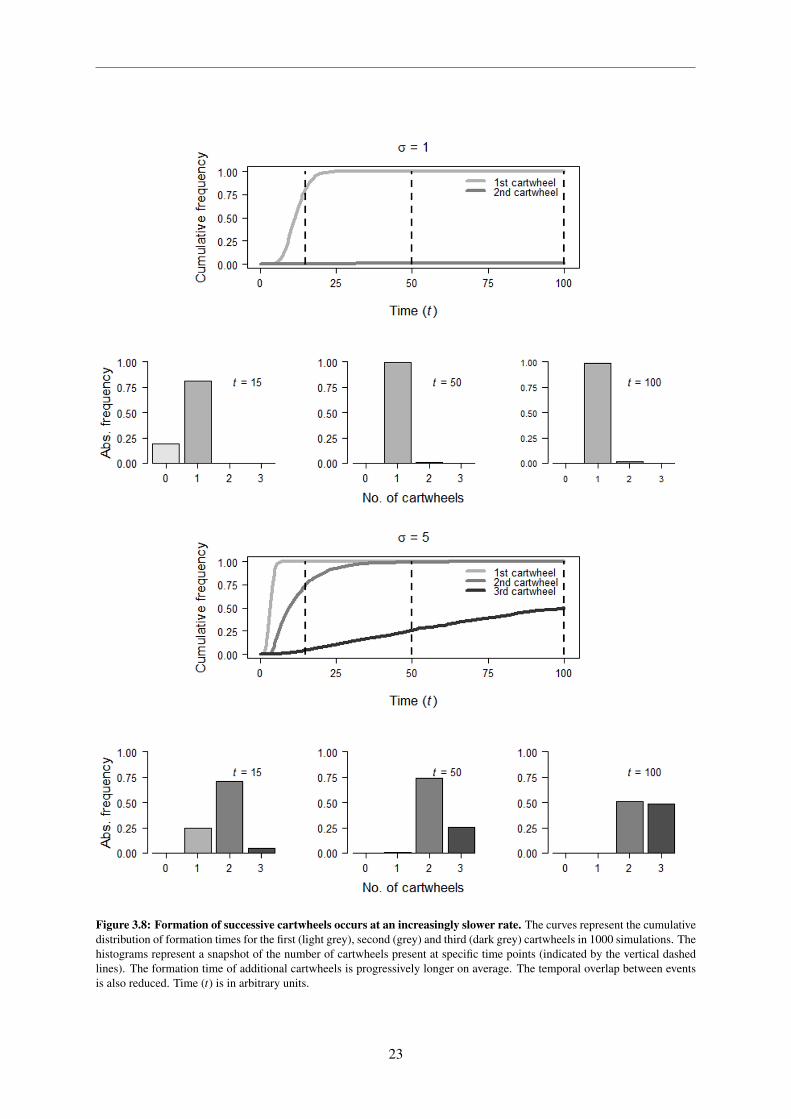
Figure 3.8: Formation of successive cartwheels occurs at an increasingly slower rate. The curves represent the cumulativedistribution of formation times for the first (light grey), second (grey) and third (dark grey) cartwheels in 1000 simulations. Thehistograms represent a snapshot of the number of cartwheels present at specific time points (indicated by the vertical dashedlines). The formation time of additional cartwheels is progressively longer on average. The temporal overlap between eventsis also reduced. Time (t) is in arbitrary units.
23

Figure 3.9: The average and variance in the number of stacked rings in each cartwheel increases with time. The mainplots show the time evolution in the average number of stacked rings for 1000 simulations of the reference and high influxconditions. The cumulative distributions represent the number of rings present at specific time points (indicated by the verticaldashed line). In the reference condition, only the first cartwheel reaches linear growth on average. In the high influx conditionboth reach linear growth but there is a size difference between the first and second cartwheels. The cumulative distributionsshow that the variance in the number of stacked rings also increases with time. Time (t) is in arbitrary units.
quantify this directly as we did not distinguish between stacks of different length. As we purposely did
so to avoid technical complications, we devised an approximate solution which consists of defining the
first and second cartwheels as distinct chemical species. Despite more than two cartwheels forming on
the high influx scenario, considering just the first two is sufficient for comparison purposes.
The results in Fig. 3.9 show the average number of stacked rings and their distribution at specific time
points for the reference and high influx conditions. In the reference condition, as the second cartwheel
seldom forms and when it does it takes a long time, its average elongation rate is very slow. Concerning
the high influx condition, stacking occurs on the first cartwheel until the second is formed. Then, the
average elongation rate of the first cartwheel slows down and eventually approaches the value of the
second one. The longer it takes for the second cartwheel to form, the larger will be the length difference
between it and the first one. It is also noticeable from the distributions at the three time points that
as the stacks become longer on average there is also a larger variance in the number of stacked rings.
These results allow us to derive some general properties regarding the model. First of all, there is an
average difference in length between cartwheels, with the ones that form earlier being longer than the
ones that form later. Secondly, the elongation rate is bounded by the input and depends on the number of
cartwheels that are present, otherwise the elongation rate of the first cartwheel would not be reduced by
24

Figure 3.10: Stacking is determinant for inhibiting cartwheel formation. The points represent the logarithm of the forma-tion time of the first (light grey) and second (dark grey) cartwheels in each of the 1000 simulations. The parameter values notindicated in the x-axis were set to 1. σ – the formation time of both cartwheels and the delay between events decreases forhigher values of the parameter; kon – the delay between formation of the first and second cartwheels decreases for higher valuesbut apparently reaches a minimum value; koff – while higher values increase the delay between the two formation events, thedelay is still present for relatively lower values of the parameter; ks – increasing the stacking rate substantially increases theformation time of the second cartwheel while lowering it below the reference value decreases it. Note that both axes are in logscale.
the formation of the second one. Third, longer cartwheels on average should have a wider distribution
of lengths.
3.5.3 Parameter dependence of cartwheel formation and elongation
The analysis performed on these two scenarios provided insights regarding the general dynamics of the
model. However, they are insufficient to understand how each parameter contributes to the output of the
model. So, to gain a broader understanding, we asked how cartwheel formation depends individually on
each parameter. On more practical terms, what are the formation times of the first and second cartwheels
in a range of values for a given parameter? In order to answer this question, we ran 1000 independent
simulations up to t “ 1000 and extracted the times at which each cartwheel formed (Fig. 3.10). The
values for the parameters in question were chosen to best illustrate the change in the time distributions
of both formation events. The remaining parameters were set to a value of 1.
For higher values of σ the formation times of both the first and the second cartwheels are shorter and
less disperse. Moreover, both distributions become increasingly similar for higher values of σ . There is
still an average difference of about one order of magnitude between formation of the first cartwheel and
formation of the second one up to σ “ 10. For lower values of σ the time of formation of the second
cartwheel can be so long that the event does not occur in the simulations. These results are contrary to
what was observed in the linear model. While increasing the production rate does accelerate formation
of both the first and second cartwheels, the relative difference between the two is not constant and is
actually shortened for high σ .
Regarding the oligomerization rate kon, the time distributions also become more similar, as it was
observed for σ . However, the formation time of the first cartwheel seems to depend little on kon under
the chosen parameter values. This was also observed in the linear model when the diverting mechanism
25

is disabled. The fact that the results for kon “ 25 and kon “ 50 are nearly identical indicates there is
a limit on how fast cartwheel formation can get. This suggests that in the conditions tested the rate-
limiting step in the model is the availability of intermediates, which depends on σ . The same result was
observed in the linear model, as the average end product formation times in the presence and absence of
a diverting mechanism converged asymptotically, as a function of kon.
When it comes to koff a small increase is sufficient to determine that the second cartwheel only forms
in a fraction of the simulations, in the considered time window. Likewise with kon the formation times of
the first cartwheel appear to be poorly sensitive to the dissociation rate. On the other hand, when koff is
set to 0, which represents a scenario in which oligomerization is irreversible and for other values of the
parameter lower than 1 there is still a substantial difference in the formation times of both cartwheels.
This suggests koff is not necessary for inhibiting the formation of supernumerary cartwheels.
Increasing ks also delays the formation time of the second cartwheel. Conversely, decreasing ks
below the reference value has a significant effect in narrowing the difference between formation times
of the first and second cartwheels. This confirms that cartwheel formation is highly sensitive to the
stacking rate. The results also recapitulate the conclusions drawn for the linear model. Note that by
definition ks has no impact in the first cartwheel formation event; the times are kept in the graph for
reference purposes.
It should also be noted that the time lapse between production of the first and second cartwheels
can be shorter than the time until formation of the first cartwheel. This can be observed in the graph
for higher values of σ and kon. It can be explained by the fact that we considered an initial condition
in which no molecules are present, such that there is a delay in cartwheel formation associated with the
time necessary for producing sufficient intermediates.
Briefly put, these results show that cartwheel formation is more susceptible to be inhibited than
favored; the change in the distribution of formation times is much more pronounced under koff and ks
variation than in the case of kon and σ . Moreover, they confirm that stacking is the main reason why
cartwheel formation is inhibited. Lastly, the formation time of the first cartwheel varied only with the
production rate.
As cartwheel formation is affected so too should elongation be. So, we sought out to understand how
the average number of stacked rings would vary under the same conditions. We used the aforementioned
counting method to determine when a ring is added and selected a time point in which elongation had
reached linear growth (t “ 50 was a suitable choice for all cases). Then, we averaged the stacked rings
count for the number of cartwheels in each simulation to obtain individual values. The corresponding
data are plotted on Fig. 3.11. Note that when studying the dependence on kon, koff and ks, σ was fixed
to a value of 10 in order to make the changes more noticeable.
Higher values of σ lead to longer cartwheels, in spite of more structures also forming. This is
in line with previous observations that the model shows a tendency towards cartwheel elongation in
detriment of cartwheel formation. Increasing kon on the other hand results in shorter cartwheels. This
can be explained by the fact that we have shown that increasing this rate favors cartwheel formation
and supports the notion that the influx is limiting respective to stacking, such that the pool of available
intermediates is split among existing cartwheels. The inverse can be observed when koff is varied, as
the reduction in cartwheel numbers allows the existing ones to elongate further. The extreme example
26

0
20
40
60
1 2 5 10 25 50σ
Avg
. sta
cked
rin
gs
0
20
40
60
1 2 5 10 25 50kon
0
20
40
60
0 0.1 0.51 2 5koff
0
20
40
60
0.1 0.5 1 2 5ks
Figure 3.11: Cartwheel elongation depends on the input and the number of structures that form. The points represent theaverage length of the cartwheels present in 1000 simulations at t “ 50. The parameters not indicated in the x-axis were fixedon a value of 1, except for σ which was set to 10. σ – the average number of stacked rings increases with higher molecularinflux; kon – the formation of additional cartwheels reduces stack length for higher values; koff – as cartwheel formation isinhibited by higher koff , the length of the stacks increases; ks – the same trend as koff is observed but even more extreme; lowervalues are associated with more cartwheels and consequently smaller stacks. Note that both axes are in log scale.
of this same tendency can be observed when ks is set to higher values. It is also noticeable that in
some conditions the observations seem to group together. For instance, this is discernible in the results
respective to higher koff or ks values. These reflect the underlying number of cartwheels present in that
group of simulations. In other words, if the simulations contain a more uniform distribution of cartwheel
numbers at the considered time point, this will have an impact on stack length with the simulations
where more individual cartwheels arose showing shorter stacks and vice-versa for the ones where fewer
cartwheels formed. These are more evident in conditions where cartwheel formation is more strongly
inhibited, such that the formation of one more structure has a substantial effect on the average number
of stacked rings. Given our previous result on the delay of formation times and its consequence on
increasing the size difference between cartwheels, the variation in the number of stacked rings for a
particular set of parameters can cast insights on what happens at the individual level. In other words,
one can infer from the results that higher values of koff and particularly ks should lead to a larger variance
in stack length.
3.5.4 Molecular levels of the intermediates
We have now covered how the two countable outputs of the model – cartwheel formation and elonga-
tion – depend on the parameters. It is also expected that the parameters should influence its internal
composition, namely the distribution of intermediates. In turn, this distribution should be associated to
the rate of cartwheel formation. For example, it is expected that more higher-order structures should be
present when formation of additional cartwheels is likelier. In order to confirm this, we extracted the
27

average number of Ci molecules present at t “ 50 and calculated the proportion of the total population
of intermediates they represented. Despite the levels of the intermediates never reaching a steady-state
the proportion is relatively unchanging. The results are plotted in Fig. 3.12.
Dimers were the most abundant species (down to a minimum of 45% for kon “ 50) for all the tested
parameter sets. Contrary to the previous observation on the frequency of higher-order oligomers, in-
creasing the production rate favors cartwheel formation but it does not lead to a higher frequency of the
larger intermediates. In fact, there is a progressively larger proportion of dimers for higher σ values.
However, these species are more abundant in absolute number when compared to the other scenarios.
The results concerning oligomerization rate variation do show this trend, i.e. for higher kon the pro-
portion of larger intermediates increases. Increasing the value of koff and especially ks has the opposite
result in that higher-order oligomers become progressively rarer. In the first case this can be ascribed
to the fact that dissociation is favored instead of oligomerization. In the second case it is due to the
stacking of almost all the intermediates, such that the molecules remaining are mostly dimers that were
produced and not yet diverted. The fact that dimers come up as the most abundant species suggests the
critical step for cartwheel formation could be the binding of a C1 molecule to a C8 molecule but we did
not confirm this.
In summary, the results presented in this section highlight a number of important aspects regarding
the model: 1) cartwheel formation is eventually inhibited while the stacks keep elongating at a steady
rate; 2) the model can behave in such a way that the first cartwheel forms relatively quickly and then there
is a long waiting time for the second one to form; 3) the rate at which the second cartwheel forms depends
highly on the stacking rate ks; 4) the time to the first cartwheel formation event is highly dependent on
the production rate σ ; 5) the average length of the stacks is bounded by the production rate and depends
on the number of cartwheels that form; 6) dimers tend to be the most frequent species but conditions
which favor cartwheel formation are associated with an increase in the number of higher-order structures.
The key prediction of the model is that cartwheel numbers and stack length are strictly connected. So,
regarding the question on controlling cartwheel numbers despite fluctuations in the upstream factors, it
should be expected for instance that the system is capable of buffering increases in Plk4 concentration.
However, an augmentation in Plk4 levels that is insufficient for eliciting supernumerary cartwheels will
nevertheless result in longer stacks.
28

Figure 3.12: The distribution of intermediates is associated with cartwheel formation. The plots show the relative inter-mediate numbers at a time where its composition is relatively unchanging. Simulations were conducted using the indicatedparameter values and all others set to 1. σ – increasing the parameter leads to a higher proportion of dimers but also highernumber of molecules on absolute. kon – as the oligomerization rate is increased, the proportion of higher-order structuresincreases. koff – increasing the dissociation rate increases the prevalence of smaller intermediates. ks – higher ks determinethat dimers are increasingly prevalent up to the point they are almost the only species present.
29

30

Chapter 4
A method for estimating cartwheel length
In the previous section we characterized the dynamic behavior of a model that predicts a distribution
of cartwheel numbers and a distribution of stack lengths, which depend on time. Regarding the first,
the experimental readout for testing model predictions is measuring cartwheel formation times. The
simplest way to do this is by detecting foci of fluorescently labeled cartwheel proteins such as Sas-6
and STIL/Ana2. Regarding the second, it requires imaging longitudinal sections of the cartwheel using
electron microscopy and being able to identify the number of stacked rings [29], which should pose
more difficulties.
Therefore, we propose a method which should be able to address some of the challenges in the imag-
ing process: estimating cartwheel length through the distribution of aspect-ratios of randomly generated
cross-sections. One would have to purify cartwheels and fix them on a physical medium such that they
would orient themselves randomly. Then, by making a single section of the medium one could obtain a
large number of cartwheel cross-sections and their contours using image analysis, whose aspect-ratios
can then be calculated (Fig. 4.1). Physicists typically use the chord-length distribution of a suspension of
particles to estimate there size and shape, which can be obtained using laser diffraction and reflectance
methods, among others [42]. Our hypothesis is that length can be estimated using the aspect-ratio dis-
tribution. These are also easier to define given that the setting we proposed would yield 2D images.
Before testing whether the distributions of the aspect-ratios of cartwheel sections can be used for
estimating stack length, we ask if it is possible to distinguish between two populations of differently
sized cartwheels, i.e. stacks with different average number of stacked rings, and if so what is the required
sample size.
In order to simulate this experiment, we first designed an algorithm for generating random-cross
sections assuming that a cartwheel can be viewed as a right circular cylinder. We considered a diameter
of 123 nm and a ring height of 15 nm, based on experimental measurements for bld-12, the C. reinhardtii
homolog of Sas-6 [24]. The value used for ring height represents the lower bound in the range of natural
variability, so it is the worst case scenario when trying to distinguish between distributions containing
different numbers of stacked rings. To generate a cross-section, the algorithm proceeds by generating
three coordinates x,y and z within the cylinder to determine its origin. The orientation of the cross-
section can then be obtained by generating three values for the Euler angles α , β and γ (Fig. 4.2. This
yields a cross-section which is circular when it is parallel to the base of the cylinder, rectangular when
it is perpendicular, elliptic when it is oblique and semi-elliptic when it does not go through both the
top and the base of the cylinder. We ignored tangent sections producing points or straight lines. The
aspect-ratio of these shapes can then be calculated by dividing the length of the major axis by that of the
minor axis.
To answer whether we could distinguish between different cartwheel length distributions, we gen-
erated two study sets by running 1000 simulations of the model described in the previous section and
31

Figure 4.1: Cylindrical contour of the cartwheel and possible cross-sections. A - Cylindrical contour of a 5-layeredcartwheel model; B - Illustration of possible cross-sections of a cylinder and the resulting 2D shapes. The proposed experimentshould yield a distribution of cartwheel sections whose masks would be similar to the shapes presented here. The aspect ratioof these shapes was defined as the length of the major axis (M) over the length of the minor axis (m).
Figure 4.2: Example of a random cross-section obtained with the algorithm. The point P is generated by randomlyselecting values for the x,y and z coordinates and defines the origin of a x´ y´ z plane of reference. The plane is then rotatedinto a new X ´Y ´Z frame using the three Euler angles. α is the angle between the x-axis and a vector N which defines theintersection of the rotated frame with the xyz plane. β is the rotation between the z and Z axis. γ is the rotation between N andthe y-axis. The section obtained is the represented by the colored ellipse.
32

Figure 4.3: Aspect ratio distributions and power analysis. A – Comparison between » 4 (σ “ 1) and » 5 (σ “ 1.2)stacked rings on average. B – Comparison between » 9 (σ=2) and » 10 (σ “ 2.2) stacked rings on average. Cartwheelsize distributions were obtained from 1000 simulations of the model at t “ 50 using the indicated production rate and allother parameters with a value of 1. Aspect ratio distributions were obtained by using the described algorithm. Power wasestimated by performing 1000 Kolmogorov-Smirnov tests using sub-samples of a certain size and determining the proportionof rejections. The differences between both distributions in A is larger than B, correspondingly yielding a smaller sample sizeto reach the stipulated power level.
retrieving the distribution of stacked rings at t “ 50. Each study set contains two distributions which
vary by approximately one stacked ring: approximately 4 vs. 5 rings in one case and 9 vs. 10 in the
other. The aspect-ratio distributions were obtained in two steps: first, by randomly selecting a cartwheel
of a given length based on its frequency in the distributions and then running the algorithm described
above. Finally, we conducted a power analysis by taking 1000 samples from both distributions for each
of the study sets and determining the proportion of Kolgomorov-Smirnov test rejections. We repeated
this procedure for a range of sample sizes and used a power value of 80% to conclude if a given sample
size was sufficient to distinguish between the distributions (Fig. 4.3).
It can be observed that a sample size of 150 is sufficient to cross the 80% threshold in the first study
set while a much larger sample size (» 900) is required in the second. This suggests that the aspect-ratio
of the cross-sections does not vary linearly with the number of stacked rings. An explanation for this is
that as cartwheels are longer the probability of finding a transverse section also increases. To confirm
this and to test whether the aspect-ratio of the cross-sections could be used to estimate stack length, we
generated cross-section distributions from cartwheels of known length and used the average aspect-ratio
as a measure of those distributions (Fig. 4.4). As a reference, we covered the size variation measured
in C. reinhardtii cartwheels [29]. The results show that average-aspect ratio decreases with some power
33

2 4 6 8 10 12
1.5
2.0
2.5
3.0
3.5
4.0
Stacked rings
Ave
rage
asp
ect−
ratio
Figure 4.4: Average aspect ratio as a function of cartwheel size. The observations correspond to the average aspect ratio ofdistributions in heights (in nm) which range from one quarter to double that of the ring diameter, and are also representative ofthe natural variation found in Chlamydomonas. Each stacked ring corresponds to a height of 15 nm.
of the number of stacked rings and not linearly. This allows us to conclude that at least for cartwheels
containing only a few stacked rings the average aspect-ratio of the cross-sections can be used as an
estimator of stack length. It has been reported that human cartwheels typically occupy approximately
100 nm of the proximal region of the centriole [3], which would correspond to 6-7 stacked rings, so the
method would be adequate to detect variation around this value.
Note that we are assuming an ideal scenario for this experiment regarding cartwheel and cross-
section identification. Our proposition implies isolating centrioles, which is possible through ultra-
centrifugation [43], and/or cartwheels. On the analysis side, it is also assumed that one is able to retrieve
the correct contour from all possible cross-sections. Experimental testing is required for assessing its
feasibility. Notwithstanding all these issues, our focus was on analyzing the method from a theoretical
perspective and we have shown that it is adequate for estimating stack length.
34

Chapter 5
Discussion
We begin this section by reviewing the main results presented in this dissertation. The analysis we con-
ducted on the linear model shows that the probability of forming the end product for any given molecule
can be very small if it has to overcome a number of intermediate steps, at all of which it can be diverted.
When molecular influx is considered, we have shown that there is still a several-fold difference in end
product formation times when the diverting mechanism is either enabled or disabled. Likewise, for the
second-order model, the stacking mechanism is highly efficient in inhibiting cartwheel formation. After
a certain number of cartwheels have formed, depending on the parameter values, the rate at which new
ones arise is much slower. The stacks on the other hand keep elongating at a steady rate. The results
suggest that there is a trade-off between forming new cartwheels and their elongation, such that if there
is an increase in the influx which does not result in a significantly higher number of cartwheels the stacks
are expected to be longer. Our analysis also shows that if cartwheel formation is asynchronous then it is
expected there is a length difference between the individual stacks. In other words, cartwheels that are
produced earlier are longer than the ones produced later on. The distribution of intermediates is also re-
lated to cartwheel formation with higher-order oligomers becoming more prevalent in conditions where
cartwheel formation is more favorable. Regarding the method we suggested for addressing cartwheel
length, our analysis shows that it is theoretically possible to distinguish between two differently-sized
cartwheel populations even if the difference is minimal. The sample size for doing so is smaller if the
cartwheels are also shorter. We have also shown that the average aspect-ratio can be used as an adequate
estimator of cartwheel length for a range of values.
5.1 Model assumptions
The assumption that cartwheel formation and stacking are irreversible determines that each molecule
which is produced will end up either as part of a new cartwheel or stacked on top of a preexisting
one. However, there is some evidence which supports that cartwheel structure may be more dynamic.
In human cells, the cartwheel is only present at the procentriole and disappears in the later stages of
centriole development as Sas-6 and STIL are de-localized from the centrosome [44]. The cartwheel
in Chlamydomonas undergoes length variation across the cell cycle [29]; the same has been reported
for Spermatozopsis [30]. The cause of these alterations is not known. They may occur due to active
degradation of the rings or fluctuations in Sas-6 expression associated with cartwheel instability. On
the other hand they can represent exceptions as similar phenomena have not been reported for other
systems. In spite of this, we could still ask if adding reversibility to cartwheel formation and stacking
would change the results. Doing so is not so straightforward considering our methodology. It would
imply adding more parameters to the model to reflect ring and stack dissociation. Also, in practical
terms, we would have to consider all different-sized cartwheel species explicitly, which could require
35

using a different software tool for conducting simulations.
We imposed no limits on cartwheel numbers nor stack length when defining the model, such that both
keep growing with time. However, we considered that stacking does not occur on the cartwheel present
at the mother centriole, implying that the process is somehow arrested. There may be spatial constraints
on the process or other factors in centriole biogenesis such as the onset of microtubule nucleation or
centriolar capping could influence stack elongation. CPAP, a protein which promotes microtubule poly-
merization by recruiting γ-tubulin, and CP110, a capping protein have been shown to play antagonistic
roles in promoting or inhibiting centriole elongation [45]. It is possible that these or other similar pro-
teins also affect cartwheel length. If this is true and their action is concurrent to cartwheel assembly it
may be necessary to include them in the model. Nevertheless, when applying the model to a biologi-
cal scenario, one would have to consider that cartwheel formation typically occurs during G1/S-phase,
which should place temporal constraints on the process. Therefore, by considering this time-window, it
could also be the case that the stacking mechanism is sufficient to predict both cartwheel numbers and
length in spite of other extraneous factors. Ultimately, further work is necessary for addressing all these
possibilities.
The fact that we considered that cartwheel assembly depends exclusively on Sas-6 is also a sim-
plification. As we have mentioned, it has been shown that cartwheel formation may depend on other
factors aside from Sas-6 self-oligomerization [26, 27]. Even if this is true the model may still prove
valid if these are not limiting with respect to Sas-6, as the reactions can be simplified as depending on
Sas-6 alone. Though we could have considered Ana2 instead of Sas-6, the same structural role has not
been shown for its human homolog STIL nor for any other as far as we know. Moreover, aside from
C. elegans the ninefold symmetry of the cartwheel, and more specifically, of the Sas-6 rings, is highly
conserved [46]. This makes Sas-6 an interesting candidate if the model is to be generalized to a variety
of systems. On the other hand, if any other unknown factor is the limiting one in cartwheel assembly
but it retains the ninefold stoichiometry, one would simply have to restate that each of the components
in the model represents an i-mer of that species.
Regarding the stacking mechanism, it remains highly hypothetical. Sas-6 has been shown to oligomer-
ize and form stacks in vitro, with varying symmetry [47], but the distance between stacked rings appears
to be smaller than in vivo (» 4 nm vs. »8 nm). This suggests other proteins can be responsible for
organizing the stacks, with a likely candidate being Bld10/Cep135, which binds to the pinheads of the
spokes [48]. If Bld10 is not limiting relative to Sas-6, as we have mentioned, the model may still be
valid in its current state. Alternatively, if it is limiting, Bld10 also exhibits ninefold organization [16],
so the model can perhaps be adjusted to this context. At the moment, quantitative analyses are incon-
clusive as to which one is limiting[10]. A more vehement issue arises regarding the stacks forming by
successive addition of intermediates. It could be that rings are formed elsewhere and only afterwards
piled on top of the cartwheel. In fact, some have suggested that the centriolar lumen acts as the template
for cartwheel ring formation, with the structure then being transported to its typical location near the
wall of the mother centriole. This claim is based upon the existence of a Sas-6 focus inside the centriolar
lumen [26]. However, the evidence is not conclusive. If cartwheels are indeed formed in the centriolar
lumen, then there would have to be a transport mechanism which is of yet to be identified. Experimen-
tal evidence of the assembly mechanism could be obtained using electron microscopy. For example,
36

considering these two hypotheses, in principle one should be able to observe a ring in the process of
binding to a stack, or a ring being formed on top of it. To the best of our knowledge, this is yet to be
shown. What is definitely known is that the stacks occur in vivo. Therefore, without further information,
the assumption that they are formed by progressively stacking intermediates on top of the cartwheel is a
possible explanation on how stacking can happen.
If we had considered steric constraints in the stacking mechanism its efficiency in inhibiting cartwheel
formation could be reduced. In other words, the ability of a cartwheel to divert intermediates could be
limited. On the other hand, this opens up a lot of considerations. There can be also steric constraints
on the binding of intermediates, which could affect their oligomerization properties. Ultimately, includ-
ing steric constraints would imply modeling molecular structure, which would take an entirely different
approach.
Finally, we considered stacking to be unidirectional mainly because the cartwheel typically forms
orthogonally to the mother centriole. Also, there is some evidence that its components may be chiral,
but it is not known if this property arises from Sas-6 or the pinhead forming Bld10 [16]. It has also been
proposed that cartwheel formation may be bi-directional in bryophytes [16]. Nevertheless, judging from
our results this would only determine that stacking would be even more efficient in inhibiting formation
of more than one cartwheel.
5.2 Approach on model analysis
The mathematical analysis we performed on the linear model allowed us to fully characterize its dynamic
behavior. The expressions we have derived not only describe the equilibrium condition but also the
temporal evolution of the system. In this way, we were able to quantify how the formation of the end
product depends on the parameters. The main shortcoming of this system is that it does not allow us to
explicitly analyze how cartwheel formation reduces the formation rate of the next one, i.e. we are only
able to distinguish between absence and presence of a diverting mechanism but not a scenario where
there is a transition between a state in which there is no diversion but it is eventually enabled as the end
product is formed. Additionally, it does not take cartwheel elongation into account. Nevertheless, it
allowed us to understand the importance of the length of the sequence and the diverting mechanism in
inhibiting end product formation, and these features are retained in the more complex model.
On the other hand, the model which considers second-order oligomerization and stacking is not so
easily tractable and it does not reach a steady-state. The analysis we conducted through simulations
limited us to key sets of parameter values in other to illustrate their influence on cartwheel formation
and elongation and we could only obtain approximate results. While this is sufficient to draw general
conclusions regarding model dynamics it is not an ideal scenario, especially in the possibility of fitting
the model to experimental results, though in this case methods such as Approximate Bayesian Compu-
tation [49] can be employed. An alternative to this simulation-oriented approach could be through the
use of methods such as finite-state projection [50] which can provide approximate solutions for models
which cannot be solved analytically. Nevertheless, running simulations of this model does not come
with a high enough computational cost which would deem other strategies to be strictly necessary. Since
we would not be able to obtain analytical solutions this approach was considered to be the most effective
37

for the purposes of this dissertation, even more so given that the Gillespie algorithm is implemented in
Snoopy.
Finally, we also chose to look at the parameters in relative terms. The dissociation constants for
the Sas-6 N-N terminal interaction have been experimentally measured [24] and we could have used
to supply values for the oligomerization parameters. Likewise, experimental measurements of cellular
or centrosomal Sas-6 concentrations [25] could be used with respect to the production rate. Regarding
the first, we could not have a similar guess for the other parameters neither we could be sure that those
measurements accurately depict what occurs in vivo, as they were obtained in vitro using truncated Sas-
6 N-termini. Regarding the second, using a production reaction occurring at exponentially distributed
times rather than a constant pool of molecules allowed us to address stochasticity in the source directly,
which was one of the main premisses of the problem we sought to answer. Nevertheless, a physical scale
for the parameters should be taken into account in the future.
5.3 Perspectives on centriole biogenesis
The main conclusion of this dissertation is that the proposed stacking mechanism of cartwheel assembly
can inhibit the formation of more than one structure and is highly efficient in doing so. By extension, this
mechanism can also explain how centriole numbers are strictly controlled by the cell provided that the
cartwheel is indeed the key step which establishes a centriole. Our depiction of the stacking mechanism
also enables cartwheel elongation by the successive addition of stacked rings. Thus, there is an interplay
between the number of cartwheels and the length of the stack.
Testing the model implies measuring cartwheel formation and elongation rates, or alternatively
cartwheel numbers and stack length. The critical consideration here is that one is able to experimentally
control protein levels. More specifically, manipulating Sas-6 concentration by directly affecting its ex-
pression should correspondingly have implications for the input parameter, and likewise for Plk4 given
our assumption that Sas-6 levels are a monotonously increasing function of its concentration. This can
provide an experimental setting in which the model can be tested. For example, Sas-6 overexpression
should be interpreted as a higher production rate. This places a constraint on model dynamics which
in association with a given time-window can allow one to infer properties of the assembly process. On
more practical terms, this means fitting the model to different sets of experimental data and estimat-
ing values for the parameters. Ascribing physical meaning to the parameters can suggest whether or
not other factors should be at play. For instance, if the model predicts much stronger oligomerization
dynamics than the ones measured in vitro it supports the notion that other factors may contribute to
cartwheel assembly.
The fact that the model predicts cartwheel numbers and length widens the realm of possibilities. For
example, it could be that the model is able to correctly predict cartwheel numbers but not stack length
or the other way around. This would suggest other factors to be at play. In summary, by studying the
conditions in which the model succeeds or fails in predicting experimental data can assist in unraveling
more of the centriolar assembly process. Failure in producing accurate predictions can be a result of
upstream factors or insufficiency of the oligomerization/stacking dynamics. Further work should be
done to study all these conditions and their implications but that is beyond the scope of this dissertation.
38

For now, we have established what is the outcome of the model in different conditions which in its turn
should facilitate the interpretation of these analyses.
It should also be noted that despite not having considered spatial information when defining the
model, the formation and elongation of a stack implies the existence of a physical structure which con-
centrates Sas-6. Therefore, if one is to fluorescently label Sas-6, or possibly other cartwheel markers,
and is able to link a focus of these proteins to a certain number of cartwheels, quantifying fluorescence
intensities can also be used as a readout for the model. For example, if a series Sas-6 foci correspond to
single cartwheels, different fluorescence intensities should be associated to different protein concentra-
tions, which in turn could indicate stacks of varying length. This requires enough imaging resolution to
be able to accurately distinguish the foci and it also implies that all the proteins are indeed part of the
stack. We did not delve into the technical aspects but this is theoretically possible.
Despite having discussed the model in the light of centriole duplication and formation of supernu-
merary centrioles which can arise from artificial Plk4 overexpression [9] it does not rule by definition
natural de novo biogenesis. This process is characteristic of terminally differentiated multicilliated cells,
where multiple centrioles are synthesized to form the basal bodies of the cilia [4]. However, in a setting
which allows for both supernumerary centrioles to arise at the centrosome and also de novo biogenesis
it is most likely that spatial resolution is necessary to distinguish the two. Otherwise, the model can still
be applied to predict centriole numbers.
As we have mentioned, the stacking mechanism provides an explanation on how the cartwheels
form as a multi-layered structure but we do not claim this process depends on Sas-6 alone. A recently
published article concludes that Sas-6 self-oligomerization is insufficient to ensure efficient cartwheel
formation and that the presence of a cylindrical scaffold, based on an electron-dense region found in
Trichonympha cartwheels called the cartwheel inner densities, can not only account for this but also de-
termines that Sas-6 rings assemble orthogonally to a surface where the scaffold is placed [51]. However,
the authors acknowledge that Sas-6 oligomerization may be assisted by post-translational modifications
or other centriolar components. Moreover, when it comes to cartwheel numbers their results imply the
existence of one scaffold per cartwheel. As they did not explore the biochemical nature of these scaf-
folds it is not clear what they represent in terms of the centriolar biogenetic process. Either way, if Sas-6
self-oligomerization is indeed insufficient to explain how rings are formed, that is not inconsistent with
the model we have proposed. We simply assumed Sas-6 was limiting but other processes could be in-
volved. However, if a scaffold is required for cartwheel assembly, then the number of cartwheels could
be limited by the number of scaffolds and not any type of assembly dynamics.
We have shown that the suggested method for estimating cartwheel size based on the aspect-ratio
distribution of random cross-sections is theoretically adequate. On practical terms it is highly depen-
dent on the ability to extract the masks one would expect from cylindrical sections out of cartwheel
sections. Since the cartwheel is not exactly shaped like a cylinder this may not be trivial, especially if
a given section would capture only a small portion of the cartwheel. Centrioles can be purified through
ultra-centrifugation [43] but it may be necessary to isolate the cartwheels. All these considerations de-
termine that experimental testing of this method is ultimately necessary. We cannot dismiss the fact that
the method may prove insufficient if cartwheels contain a significantly large number of stacked rings,
more precisely over 10-12, which can be expected in the very least for Trichonympha cartwheels [28].
39

Nevertheless, there are other measures which come from this method and could be used to complement
length estimation. For example, calculating the aspect ratios of cross-section implies measuring its ma-
jor and minor axes and the maximum length of the major axis of a cross-section depends on cartwheel
length. We did not explore these alternative measures but they are a consequence of the analysis method
and therefore readily available. On the other hand, the applicability of this method can extend beyond
cartwheel length estimation, in principle. Centrioles, for instance, are cylindrical in shape and can be
purified [43]. Measuring centriole length through common electron microscopy techniques [52] can be
technically demanding. The method we have suggested should provide a simpler alternative for reaching
the same goal.
40

Chapter 6
Concluding remarks
We proposed a fundamental principle which can explain how the cell controls cartwheel numbers and
consequently centriole numbers. Our theoretical analysis of the linear model shows that the length of the
sequence of intermediates in the presence of a diverting mechanism significantly reduces the probability
of forming the end product. It is also shown that even under a constant influx of molecules the diverting
mechanism can account for a substantial difference in the rate of end product formation. The results
for the second-order model show that the postulated stacking mechanism is highly efficient in ensuring
that one and only one cartwheel forms in a given time interval. Moreover, the diversity in cartwheels
numbers at a given time is reduced, suggesting it also to be robust. By determining the formation
times for the first and second cartwheels we showed that a slight increase in the stacking rate can have
substantial consequences in slowing down the assembly of supernumerary cartwheels. We also confirm
that the input of the system is critical for its outcome but stacking can still account for a considerable
degree of variation in the production rate. In our analysis, we depict a number of scenarios which reflect
both internal changes in the composition of the system we have modeled but also on its outcome, which
allowed us to derive some of the biochemical implications which could be at play at a real system.
The main consequence of our hypothesis is that cartwheels have a length distribution which is as-
sociated to its numbers. Our results suggest that if cartwheel production is asynchronous then it is also
expected that individual cartwheels show a length difference in the same system. Experimental data in
cartwheel length variability is scarce, but our results show that it can be a consequence of the assem-
bly process. If our hypothesis is correct, there may also be some undisclosed physiological meaning
regarding cartwheel length.
Additionally, we suggested some strategies which can be used to test our quantitative predictions.
Testing the model is predicated on the ability to correlate both cartwheel/centriole numbers and stack
length, and also the underlying biochemical mechanisms. We have proposed an experiment which cir-
cumvents some of the technical issues in estimating cartwheel length. Our results show that even in
extreme cases in which length differences between two populations are minimal they can be detected by
comparing the aspect ratio distributions of random cross-sections.
The work developed over the course of this dissertation should cast new insights on centriole bio-
genesis and it raises the possibility that cartwheel stacks may have a length distribution. Further work
should focus on experimentally addressing model predictions and fitting in order to uncover more of the
centriole biogenetic process.
41

42

Bibliography
1. Azimzadeh, J. Exploring the evolutionary history of centrosomes. Philosophical Transcations of
the Royal Society B 369 (2014).
2. Bettencourt-Dias, M. & Glover, D. Centrosome biogenesis and function: centrosomics brings new
understanding. Nature Reviews Molecular Cell Biology 8, 451–463 (2007).
3. Gönczy, P. Towards a molecular architecture of centriole assembly. Nature Reviews Molecular Cell
Biology 13, 425–435 (2012).
4. Brito, D. A. et al. Deconstructing the centriole: structure and number control. Current Opinion in
Cell Biology 24, 4–13 (2012).
5. Nigg, E. A. Origins and consequences of centrosome aberrations in human cancers. International
Journal of Cancer 119, 2717–2723 (2006).
6. Bettencourt-Dias, M. et al. Centrosomes and cilia in human disease. Trends in Genetics 27, 307–
315 (2011).
7. Nigg, E. A. & Raff, J. W. Centrioles, centrosomes, and cilia in health and disease. Cell 139, 663–
678 (2009).
8. Galletta, B. J. et al. A centrosome interactome provides insight into organelle assembly and reveals
a non-duplication role for Plk4. Current Opinion in Cell Biology 24, 4–13 (2016).
9. Lopes, C. A. et al. Plk4 trans-autoactivation controls centriole biogenesis in space. Developmental
Cell 35, 222–235 (2015).
10. Bauer, M. et al. Quantitative analysis of human centrosome architecture by targeted proteomics
and fluorescence imaging. The EMBO Journal 35, 2152–2166 (2016).
11. Wolkenhauer, O. Systems biology: the reincarnation of systems theory applied in biology? Brief-
ings in Bioinformatics 2, 258–270 (2001).
12. Dzhindzhev, N. S. et al. Asterless is a scaffold for the onset of centriole assembly. Nature 467,714–718 (2010).
13. Sonnen, K. F. et al. Human Cep192 and Cep152 cooperate in Plk4 recruitment and centriole du-
plication. Journal of Cell Science 126, 3223–3233 (2013).
14. Ohta, M. et al. Direct interaction of Plk4 with STIL ensures formation of a single procentriole per
parental centriole. Nature Communications 5 (2014).
15. Cottee, M. A. et al. SAS-6 oligomerization: the key to the centriole?. Nature Chemical Biology 7,653–653 (2011).
16. Hirono, M. Cartwheel assembly. Philosophical Transactions of the Royal Society B 369 (2014).
17. Rogers, G. C. et al. The SCF Slimb ubiquitin ligase regulates Plk4/Sak levels to block centriole
reduplication. Journal of Cell Biology 184, 225–239 (2009).
43

18. Uetake, Y. et al. Cell cycle progression and de novo centriole assembly after centrosomal removal
in untransformed human cells. Journal of Cell Biology 176, 173–182 (2007).
19. Zitouni, S. et al. Cdk1 prevents unscheduled Plk4-STIL complex assembly in centriole biogenesis.
Current Biology 26, 1127–1137 (2016).
20. Woodruff, J. B. Pericentriolar material structure and dynamics. Philosophical Transactions of the
Royal Society B 369 (2014).
21. Pimenta-Marques, A. et al. A mechanism for the elimination of the female gamete centrosome in
Drosophila melanogaster. Science 353 (2016).
22. Dong, G. Building a ninefold symmetrical barrel: structural dissections of centriole assembly.
Open Biology 5 (2015).
23. Pukowski, A. et al. The SCF–FBXW5 E3-ubiquitin ligase is regulated by PLK4 and targets HsSAS-
6 to control centrosome duplication. Nature Cell Biology 13, 1004–1009 (2011).
24. Kitagawa, D. et al. Structural basis of the 9-fold symmetry of the centrioles. Cell 144, 364–375
(2011).
25. Keller, D. et al. Mechanisms of HsSAS-6 assembly promoting centriole formation in human cells.
Journal of Cell Biology 204, 697–712 (2014).
26. Fong, C. S. et al. SAS-6 assembly templated by the lumen of cartwheel-less centrioles precedes
centriole duplication. Developmental Cell 30, 238–245 (2014).
27. Cottee, M. A. et al. The homo-oligomerisation of both Sas-6 and Ana2 is required for efficient
centriole assembly in flies. eLife eLife 4 (2015).
28. Guichard, P. et al. Native architecture of the centriole proximal region reveals features underlying
its 9-fold radial symmetry. Current Biology 23, 1620–1629 (2013).
29. O’Toole, E. T. & Dutcher, S. K. Site-specific basal body duplication in Chlamydomonas. Cy-
toskeleton 71, 108–118 (2014).
30. Lechtreck, K. F. & Grunow, A. Evidence for a direct role of nascent basal bodies during spindle
pole initiation in the green alga Spermatozopsis similis. Protist 150, 163–181 (1999).
31. Mackey, M. C. & Maini, P. K. What has mathematics done for biology? Bulletin of Mathematical
Biology 77, 735–738 (2015).
32. Turing, A. The chemical basis of morphogenesis. Philosophical Transactions of the Royal Society
of London 237, 37–72 (1952).
33. McKeithan, T. W. Kinetic proofreading in T-cell signal transduction. Proceedings of the National
Academy of Sciences of the United States of America 92, 5042–5046 (1995).
34. Hopfield, J. J. Kinetic proofreading: a new mechanism for reducing errors in biosynthetic processes
requiring high specificity. Proceedings of the National Academy of Sciences of the United States
of America 71, 4135–4139 (1974).
35. Jahnke, T. & Huisinga, W. Solving the chemical master equation for monomolecular reaction sys-
tems analytically. Journal of Mathematical Biology 54, 1–26 (2007).
44

36. Gillespie, D. A general method for numerically simulating the stochastic time evolution of coupled
chemical reactions. Journal of Computational Physics 22, 403–434 (1976).
37. Koch, I., Reisig, W. & Schreiber, F. Modeling in systems biology–the Petri net approach (Springer,
2011).
38. Rohr, C. et al. Snoopy–a unifying Petri net framework to investigate biomolecular networks. Bioin-
formatics 26, 974–975 (2010).
39. Bettencourt-Dias, M. et al. SAK/Plk4 is required for centriole duplication and flagella develop-
ment. Current Biology 15, 2199–2207 (2005).
40. Marshall, W. F. Stability and robustness of an organelle number control system: modeling and
measuring homeostatic regulation of centriole abundance. Journal of Biophysics 93, 1818–1833
(2007).
41. Peel, N. et al. Overexpressing centriole replication proteins in vivo induces centriole overduplica-
tion and de novo formation. Current Biology 17, 834–843 (2007).
42. Okpeafoh, A. S. et al. Estimation of particle-size distribution and aspect-ratio of non-spherical
particles from chord length distribution. Chemical Engineering Science 123, 629–640 (2014).
43. Reber, S. Isolation of centrosomes from cultured cells. Methods in Molecular Biology 777, 107–
116 (2011).
44. Arquint, C. et al. Cell-cycle-regulated expression of STIL controls centriole numbers in human
cells. Journal of Cell Science 125, 1342–1352 (2012).
45. Schmidt, T. et al. Control of centriole length by CPAP and CP110. Current Biology 19, 1005–1011
(2009).
46. Carvalho-Santos, Z. et al. Stepwise evolution of the centriole assembly pathway. Journal of Cell
Science 123, 1414–1426 (2010).
47. Van Breugel, M. Structures of SAS-6 Suggest Its Organization in Centrioles. Science 331, 1196–
1199 (2011).
48. Van Breugel, M. et al. Structure of the SAS-6 cartwheel hub from Leishmania major. eLife eLife3 (2014).
49. Tavaré, S. et al. Inferring coalescence times from DNA sequence data. Genetics 145, 505–518
(1997).
50. Munsky, B. & Khammash, M. The finite state projection algorithm for the solution of the chemical
master equation. Journal of Chemical Physics 124 (2006).
51. Klein, H. C. et al. Computational support for a scaffolding mechanism of centriole assembly.
Scientific Reports 6 (2016).
52. Jana, S. C. et al. Mapping molecules to structure: unveiling secrets of centriole and cilia assembly
with near atomic resolution. Current Opinion in Cell Biology 26, 96–106 (2014).
53. León, K. et al. A general mathematical framework to model generation structure in a population
of asynchronously dividing cells. Journal of Theoretical Biology 229, 455–476 (2004).
45

46

Appendices
47


Methods
In this section we provide a short description of the Petri net formalism and of the Gillespie algorithm,
used for conducting model simulations. Additionally, we describe the methods used for confirming the
expressions derived for the linear model (Section 3.2).
Petri nets
Petri nets are a formalism designed by Carl Adam Petri which is often used to visually represent chem-
ically reacting systems. They can be defined by a set of places, which depict chemical species in the
system and are represented by circles, and a set of transitions, which correspond to the reactions and
are represented by boxes. Transitions have inputs and outputs which are represented by arcs, or edges,
which in the first case connect a place to a transition and in the second a transition to a place. In other
words, they indicate which of the participating species in a given reaction act as reactants or as products.
Arcs carry weights which indicate the number of tokens consumed or produced by a given transition.
The last static component in a Petri net are tokens, which represent individual entities of a given species
(i.e. molecules). A certain configuration of these tokens in the Petri net constitutes a marking, or state,
in the system [37]. Coupling Petri net visualization methods with a simulation algorithm, the system
can be evaluated dynamically. Both these features are included in the Snoopy software [38].
We used Petri nets for representing the model and the accessory simplifications. Despite the consid-
erably large number of species and reactions we are considering in the model, since we are considering
a small set of reaction categories (production, oligomerization, dissociation and stacking), using a Petri
net allows us to provide a visual aid for all the possible combinations of species. For the simplifications,
we can clearly illustrate a chain of successive events.
Gillespie algorithm
The Gillespie algorithm, or stochastic simulation algorithm, was designed by Daniel Gillespie to nu-
merically simulate reaction systems, mainly as a solution to cases where the time-evolution of a given
system could not be resolved analytically. The algorithm is mathematically consistent with the stochas-
tic formulation of chemical kinetics, which represents chemically reacting systems as Markov models.
It proceeds by determining the probability that each of the enabled reactions may occur given the current
state of the system and randomly selecting one. Then, it calculates the time at which said reaction occurs
based on an exponential distribution parametrized by the corresponding reaction rate constant. This pro-
cedure is repeated for a given number of steps or time interval (in the case of the Snoopy-implemented
version) [36].
All simulations of the model were performed using the Gillespie algorithm. Stochastic simulation
of the systems depicted in the simplifications was also used to confirm that the analytical derivations for
the linear model. For extracting formation times and the number of stacked rings, we used the single
trace export function of Snoopy, which allows us to track the result of each simulation separately.
49

Mathematical and statistical analysis
The procedure for deriving the mathematical solution to the simplified system in 3.1 was based on a pa-
per by León et al. [53].We compared the theoretical expressions in (3.3) with data simulated by Snoopy
for the respective system. For a sample size of 1000, the Kolmogorov-Smirnov test was non-significant
for all cases (p-valueą 0.05), so that we can conclude that the empirical and reference distributions are
not different. The same principle was applied in the case of (3.10). Since in this case we were comparing
categorical data, arising from different token counts, we used the Pearson χ2 goodness-of-fit test and
obtained identical results (p-valueą 0.05 for all tests). All symbolic calculations were performed using
Wolfram Mathematica. Processing of the Snoopy raw output files was performed with Python. R was
used for obtaining summary statistics and for conducting hypothesis tests. The latter were re-checked
with Wolfram Mathematica.
50

Glossary
• Cartwheel: Any Sas-6 structure containing at least one Sas-6 ring (i.e. rings and stacks).
• (Complete) Ring: Planar arrangement of nine Sas-6 dimers, formed by oligomerization. Minimal
structure which defines a cartwheel.
• Dissociation: Reverse reaction to oligomerization, producting two smaller sized intermediates.
The dissociation rate is denoted by koff .
• (Homo) Dimer: The fundamental Sas-6 species considered in the model. Molecules are produced
in dimer form.
• Influx/Production: Sas-6 dimer production into the system. A simplification of the whole process
of gene expression, translation, processing and Sas-6 dimerization. The production rate is denoted
by σ .
• Intermediate: Any of the Sas-6 species containing up to eight dimers which can either form a
complete ring (cartwheel) or be stacked on top of an existing one.
• Oligomerization: Any reaction which combines two intermediates, yielding a product containing
the number of dimers in the reactants, up to nine (size of a complete ring). Alternatively, the set
of reactions which ultimately result in cartwheel formation. The oligomerization rate is denoted
by kon.
• Stack: Any number of rings stacked on top of each other. A new ring may form on top of the
structure through building block stacking.
• Stacking: Reaction which binds intermediates to cartwheels, in a way which allows for a ring to
form stacked on top of the cartwheel. The stacking rate is denoted by ks
51