A theoretical approach to pricing leveraged loans - StudentTheses

1

EXECUTIVE SUMMARY

Specialet omhandler en teoretisk tilgang til prisfastsættelse af syndikerede lån udstedt af højt

gearede virksomheder1. Med udgangspunkt i Leland's (1994) teori for prisfastsættelse af

virksomhedsgæld udarbejdes en prisfastsættelsesmodel for sekventielt opdelt gæld. Modellen

anvendes på et case study, hvorfra priserne for de underliggende trancher i ISS' gældsstruktur

determineres. En sammenligning mellem de beregnede teoretisk priser og de egentlige

observerede markedspriser indikerer, at senior tranchen indeholder en betydelig

likviditetspræmie.

Som følge af likviditetskrisen er leveraged loan markedet blev utrolig hårdt ramt. Tidligere

tiders ekstremt høje likviditet er blevet erstattet af et stort salgspres fra såvel banker som

institutionelle investorer. Specielt market value CLOs og hedge funds har været tvunget til at

mindske deres gearing og derved sælge ud af deres porteføljer. Dette har været med til at

skabe en ubalance mellem udbud og efterspørgsel. Endvidere har den nuværende recession

betydet, at priserne er faldet endnu mere. Lån, der tidligere blev handlet omkring kurs 100,

kunne d. 31.12.2008 erhverves i omegn af kurs 60.

Fundamentet for en korrekt prisfastsættelse af leveraged loans beror på en dybdegående

forståelse af markedets drivkræfter samt strukturen på de forskellige låntyper. Leveraged loans

er typisk udstedt i forbindelse med, at et givent selskab opkøbes af en kapitalfond.

Finansieringen af gælden ydes i et fællesskab af banker på enslydende vilkår. De ledende

agentbanker har i den forbindelse tjent store fees på først at yde lånene for så efterfølgende at

sælge store dele videre i en nøje struktureret syndikeringsproces. Dette har blandt andet ført

til, at bankerne har været i hård konkurrence for at vinde mandater til at arrangere disse

omfattende gældsstrukturer. Som følge heraf er gearingen og kompleksiteten af strukturerne

på leveraged finance transaktioner blevet væsentligt forøget. Dette har været stærkt

medvirkende til lånenes betydelige forringelse efter finanskrisen begyndelse.

1 Fremover kaldet leveraged loans

2

PREFACE

This paper is a thesis for the M.Sc. in Economics and Business Administration majoring in

Applied Economics and Finance, and Finance and Accounting - both at Copenhagen Business

School. Given our specific majors, this thesis is concentrated around financial theory.

In the process of writing the thesis, we have relied greatly upon valuable insight into the

leveraged loan market. Especially industry specialists Torben Skødeberg, Capital Four

Management, and Mike Christiansen, Danske Merchant Capital, have been of invaluable help.

Without access to their institutional knowledge, it would have been extremely difficult to write

this thesis due to the privacy of the market. We would like to thank both of them very much for

their contribution. Finally, we would like to thank our advisor David Lando for his very helpful

and focused guidance. His assistance, especially in relation to the theoretical modelling, has

been essential to the contribution provided in this thesis.

Data files for the analysis are provided electronically in the back of the paper.

Enjoy your read,

Jacob and Martin

3

Table of Contents 1. PROBLEM IDENTIFICATION...................................................................................................... 6

1.1. INTRODUCTION ................................................................................................................ 6

1.2. MOTIVATION.................................................................................................................... 7

1.3. RESEARCH QUESTIONS ..................................................................................................... 8

1.4. METHODOLOGY ............................................................................................................... 8

1.5. STRUCTURE OF THESIS ..................................................................................................... 9

PART 1 ...................................................................................................................................... 11

2.1. FOUNDATION OF LOAN SYNDICATION ........................................................................... 12

2.2. ISSUERS IN THE SYNDICATED LOAN MARKET .................................................................. 15

2.3. SYNDICATION STRATEGIES IN A LEVERAGED FINANCE AGREEMENT ............................... 16

2.4. SYNDICATION PROCESS IN AN UNDERWRITTING DEAL ................................................... 17

2.5. FEE STRUCTURE.............................................................................................................. 20

2.6. SECONDARY MARKET TECHNIQUES ................................................................................ 23

2.7. CHAPTER SUMMERY....................................................................................................... 24

3. SYNDICATED LOAN FACILITIES ............................................................................................... 25

3.1. THE CAPITAL STRUCTURE OF A LEVERAGED BUYOUT ..................................................... 25

3.2. LEVERAGED LOAN CHARACTERISTICS ............................................................................. 26

3.2.1. Coupons - Floating Rate .......................................................................................... 26

3.2.2. Tenor - Maturity and Call-ability ............................................................................. 26

3.2.3. Covenants - Early Warning ...................................................................................... 27

3.2.4. Security - Lien against Assets and Shares ................................................................ 28

3.2.5. Seniority - Corporate and Legal Ranking ................................................................. 28

3.2.6. Market and Information - Private Market ................................................................. 30

3.3. LEVERAGED LOANS VERSUS HIGH YIELD BONDS ............................................................. 31

3.4. STRUCTURES OF LEVERAGED LOANS .............................................................................. 32

3.4.1. Structure of a Revolving Credit Line ....................................................................... 32

3.4.2. Structure of a First Lien Term Loan - Amortising and Institutional .......................... 32

3.4.3. Structure of a Second Lien Term Loan .................................................................... 33

3.4.4. Structure of a Mezzanine Loan ................................................................................ 34

3.4.5. Structure of a Payment-in-kind Loan ....................................................................... 35

3.5. PRICING STANDARDS...................................................................................................... 35

3.6. CHAPTER SUMMARY ...................................................................................................... 36

4

PART 2 ...................................................................................................................................... 38

4. CLO STRUCTURE .................................................................................................................... 39

4.1. FOUNDATION OF A CLO ................................................................................................. 39

4.2. PURPOSE OF THE CLO..................................................................................................... 40

4.3. CREDIT ENHANCEMENT TECHNIQUES ............................................................................ 42

4.4. HEDGE FUNDS ................................................................................................................ 48

4.5. CHAPTER SUMMARY ...................................................................................................... 50

PART 3 ...................................................................................................................................... 51

5. PRIMARY MARKET ANALYSIS ................................................................................................. 52

5.1. DEVELOPMENT IN THE PRIMARY MARKET ...................................................................... 52

5.1.1. The CLO Issuance Comes to an End ........................................................................ 54

5.2. THE IMPACT OF THE CREDIT CRISIS ON THE PRIMARY MARKET ...................................... 56

5.3. CHAPTER SUMMARY ...................................................................................................... 62

6. SECONDARY MARKET ANALYSIS ............................................................................................ 64

6.1. DEVELOPMENTS IN THE SECONDARY MARKET ............................................................... 64

6.2. THE IMPACT OF THE CREDIT CRISIS ON THE SECONDARY MARKET ................................. 66

6.2.1. Looking Into 2009 ................................................................................................... 69

6.3. CHAPTER SUMMARY ...................................................................................................... 71

PART 4 ...................................................................................................................................... 73

7.1 THE MERTON MODEL ...................................................................................................... 74

7.2. THE LELAND MODEL ....................................................................................................... 78

7.3. EXTENSION OF THE MODEL FRAMEWORK TO INCORPORATE SUBORDINATION ............. 82

7.4. CHAPTER SUMMARY ...................................................................................................... 85

8. THEORETICAL FRAMEWORK OF INPUT ESTIMATION ............................................................. 86

8.1. ESTIMATING ENTERPRISE VALUE .................................................................................... 86

8.1.1. Relative Valuation Approach ................................................................................... 87

8.2. ESTIMATING VOLATILITY ................................................................................................ 92

8.3. THE FRACTION 휶 LOST TO BANKRUPTCY COSTS ............................................................. 93

8.4. CHAPTER SUMMARY ...................................................................................................... 94

PART 5 ...................................................................................................................................... 95

9. INPUT ESTIMATION ............................................................................................................... 96

9.1. THE ISS CASE .................................................................................................................. 96

5

9.2 PEER GROUP ANALYSIS ................................................................................................... 96

9.3. ESTIMATION OF ENTERPRISE VALUE .............................................................................. 98

9.4. ESTIMATION OF VOLATILITY ......................................................................................... 100

9.5. DETERMINATION OF BANKRUPTCY COSTS, TAX, AND RISK FREE RATE .......................... 102

9.6. CHAPTER SUMMARY .................................................................................................... 103

10. THE PRICING OF ISS’S DEBT ............................................................................................... 104

10.1 PRACTICAL FOUNDATION FOR INCONSISTENCIES ........................................................ 107

10.2. THEORETICAL FOUNDATION FOR INCONSISTENCIES................................................... 111

10.3 RECAPITULATION ........................................................................................................ 112

11. CONCLUSION .................................................................................................................... 114

12. REFERENCE LIST ................................................................................................................ 118

6

1. PROBLEM IDENTIFICATION

1.1. INTRODUCTION

The high yield debt market has experienced a tremendous development in recent time. With

the entrance of leveraged loans, below-investment-grade borrowers were offered an

alternative to traditional high yield bonds. Leveraged loans soon became an important source

of financing in particular for private equity funds, since the loans were launched through a

syndication process as a private market transaction. The loan asset class rapidly became the

most compelling alternative among high yield investors, due to the distinct features of the

loans. Leveraged loans offered returns comparable to high yield bonds, but with a better

degree of principal protection. This was due to their placement in the top part of the capital

structure and in addition often secured by specific assets of the firm. Consequently, the rate of

new loan issuance clearly outpaced the new issuance of public high yield bonds in the years

preceding the credit crisis.

The leveraged loan market gained its acceptance during the days of large leveraged buyouts in

the mid-1980s. While the U.S. leveraged loan market has gradually evolved ever since, its

European counterpart did not get its breakthrough until the turn of the century. However, the

European market has gone through an incredible growth since its origin, with the experience of

the U.S. market at hand. In the very beginning, banks were the only investors purchasing the

loans to achieve their high returns. Utilising a buy-and-hold strategy, the need for a secondary

market was very limited.

However, the European loan market changed significantly with the entrance of institutional

investors. Attracted by the combination of high yields and low correlation to other asset

classes, portfolio managers had long desired the loan asset class. The CLO structure allowed

institutional investors to enter the leveraged loan market. As a consequence of their more

active investment strategies a secondary market developed - improving liquidity and

transparency. In less than a decade, institutional investors substituted banks as the dominant

market player.

Beginning in the summer of 2007, the European leveraged loan market was forced to its knees,

as the credit crisis unfolded and the global economic slowdown became more apparent. The

formerly busy primary market, characterized by large deals and elaborate structures, effectively

closed with the disappearance of overwhelming liquidity. Secondary market prices, which had

7

previously traded in a narrow band around par value, all of a sudden began to decline sharply.

With prices in steady decline and no evidence of deteriorating credit quality among highly

leveraged companies, technical market conditions seemed to be the driving force. A

comprehensive deleveraging process created a supply/demand imbalance in consequence of a

broader credit system being severely overextended. The disproportionate amount of supply

and a contracting investor base drove prices to a record low (McGaiven & Yang, 2009). As 2008

progressed, fundamental factors started to substitute the technical selling pressure and

concerns of increasing underperforming credits became ever more real. Consequently, a new

wave of falling prices accelerated in this total collapse of the leveraged loan market.

1.2. MOTIVATION

Our motivation for addressing the topic of leveraged loans is three-fold. Firstly, we want to

investigate the forces behind the rapid development of the leverage loan market. In particular,

in terms of supply and demand from private equity funds and high yield investors, respectively.

Secondly, we find it interesting to study the underlying reasons for the market's downturn

resulting from the onset of the credit crisis.

Thirdly, by observing leading leverage loan indexes trading below 60 as of 31/12/2008, loan

spreads seem to more than compensate for the most pessimistic expectations to default and

recovery rates. On the basis of this hypothesis, we wish to examine whether the market prices

reflect the actual conditions of leveraged buyouts, or if a technical created supply/demand

imbalance has distorted the price setting of leveraged loans.

8

1.3. RESEARCH QUESTIONS

In line with our motivation, this thesis addresses the following research question:

Can market prices of leverage loans be supported from a theoretical point of view?

To answer our research question we need to examine the following areas:

The characteristics of the leveraged loan market.

How a CLO is structured to deal with leveraged loans.

Institutional investors and their influence to leveraged loan market.

Influences of the credit crisis to the leveraged loan market.

A theoretical approach to pricing leveraged loans.

An implementation of the model on a leveraged buyout case.

1.4. METHODOLOGY

In the initial stage of our research we observed that leverage loan indexes were trading

historically low (McGaiven & Yang, 2009). On the basis of this observation, we formulated a

hypothesis from which the thesis takes its starting point. The hypothesis is then translated into

the main research question of the thesis.

The thesis evolves around the derivation of a model that prices the debt issued by leveraged

buyouts. This is done to provide a qualified answer to whether market prices of leveraged loans

correspond with the actual conditions of the issuing company. The model is developed on the

basis of the theoretical framework provided by Leland (1994) for pricing corporate debt. We

wish to extend his approach to incorporate subordination of debt.

In order to determine whether market prices can be supported from a theoretical point of view,

the model is tested on a case study. In continuation the model's general applicability is

discussed.

The ability to construct and subsequently apply a satisfying model for pricing leveraged loans

relies on an in-depth understanding of the leverage loan market. Consequently, the first half of

the thesis establishes a preliminary acquaintance with the overall dynamics of the leverage loan

market.

Furthermore, the ability to draw general conclusions relies on the quality of the data utilised

throughout the study. To ensure a high quality we have therefore chosen to let the study rely

9

on both primary and secondary data. The availability of relevant and updated secondary data is

to some degree limited, due to the privacy of the leverage loan market. Consequently, we have

utilised primary approaches such as informal discussions with industry specialists. In this way,

we have gathered unique knowledge essential for the study.

1.5. STRUCTURE OF THESIS

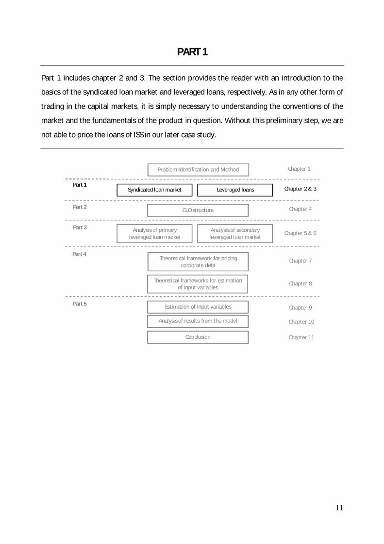
To provide a complete overview of the paper, this section highlights the structure of the thesis.

So far the introduction has identified the problem area, the underlying motivation, and the

methodology of the thesis. The following treatment of the research question is structured into

five parts which are illustrated in figure 1.1.

Figure 1.1: Structure of thesis

Source: Own creation

Part 1 introduces the reader to the characteristics of the syndication process in which the loans

are launched in the market. Furthermore, the distinct features of leveraged loans are

examined. Insight into how leveraged loans differentiate from the more traditional high yield

debt products provides the reader with a fundamental understanding of the underlying

dynamics in the market.

CLO structure

Problem Identification and Method

Estimation of input variables

Theoretical framework for pricing corporate debt

Part 1Leveraged loansSyndicated loan market

Analysis of results from the model

Part 2

Part 3

Chapter 2 & 3

Chapter 5 & 6

Chapter 7

Chapter 1

Chapter 9

Chapter 8

Chapter 4

Analysis of secondary leveraged loan market

Analysis of primary leveraged loan market

Theoretical frameworks for estimation of input variables

Conclusion

Chapter 10

Chapter 11

Part 4

Part 5

10

Part 2 entails an introduction to the fundamental CLO structure through a detailed description

of the various techniques applied. The purpose of this part is to provide the reader with a

better understand of the following analysis concerning the effects of the financial crisis on the

leveraged loan market.

Part 3 provides an in-depth analysis of the primary and secondary leveraged loan market. On

the basis of knowledge acquired from the former parts, the purpose of part three is to examine

the actual affects of institutional investors entering the leveraged loan market. This includes an

analysis of the rapid growth of the market preceding the credit crisis, followed by an analysis of

how these investment vehicles have influenced the total collapse of the leveraged loan market

as a result of the credit crisis.

Part 4 includes a presentation of a theoretical framework for pricing corporate debt issued in

connection with leveraged buyouts. On the basis of Leland (1994) the model is derived to

handle debt when tranched according to priority. Furthermore, the reader is introduced to

frameworks for estimation of model input variables.

In Part 5 the theoretical framework is tested through a case study. Before an execution of the

model can take place, the input variables must be carefully estimated. Subsequently, the results

of the model are discussed. The purpose of this part is to determine whether market prices are

in correspondence with theory. Lastly, the findings of the thesis are summarised in the

conclusion.

11

PART 1

Part 1 includes chapter 2 and 3. The section provides the reader with an introduction to the

basics of the syndicated loan market and leveraged loans, respectively. As in any other form of

trading in the capital markets, it is simply necessary to understanding the conventions of the

market and the fundamentals of the product in question. Without this preliminary step, we are

not able to price the loans of ISS in our later case study.

CLO structure






Part 2

Part 3

Chapter 2 & 3

Chapter 5 & 6

Chapter 7

Chapter 1

Chapter 9

Chapter 8

Chapter 4




Conclusion

Chapter 10

Chapter 11

Part 4

Part 5

12

2. THE ABCs OF LOAN SYNDICATION

In the following chapter the most fundamental aspects of the syndicated loan market will be

presented. At first, a brief introduction to loan syndication takes place, followed by a

description of the primary issuers and the different kinds of syndication strategies. Afterwards,

the reader is provided with a more detailed explanation of a typical syndication process in an

underwritten deal. This leads to a discussion of the associated fee structure and its major

impacts on the syndicated leveraged loan market. Finally, the chapter includes a description of

trading techniques applied in the secondary loan market.

The following chapter relies on Citigroup (2005), Gadanecz (2004), LMA (2009), LMA (2009a),

Taylor & Sansone (2006), Yang, Gupte & Lukatsky (2009). In addition to this personal

communication with Christiansen (2009) and Skødeberg (2009).

2.1. FOUNDATION OF LOAN SYNDICATION

The European syndicated loan market has experienced a tremendous development since its

origin. The syndicated loan market has evolved to become a dominant way for European

companies to access the debt markets, since it initially began taking its shape when the euro

was launched in 1999. Strongly influenced by the entrance of institutional investors, the loan

market has increasingly changed from the old bilateral bank lending relationships towards a

new world that is much more transaction and market orientated. Even though, the European

syndicated loan market is still affected by banks remaining a dominate market player, the loan

market is today much more comparable with the more traditional capital markets, such as bond

and equity markets. From this perspective, it is hard not to acknowledge the loan market’s

impact on the European corporate lending culture. However, due to the nature of its privacy,

the public in general are not familiar with the syndicated loan market and its associated lending

procedure.

“A Syndicated loan is one that is provided by a group of lenders and is structured, arranged,

and administered by one or several commercial or investment banks known as arrangers. They

are less expensive and more efficient to administer than traditional bilateral, or individual,

credit lines.” (Yang et al, 2009:7)

13

Syndicated loan arrangements entail a group of lenders that provide funds for a borrower

without joint liability. The creditors can roughly be divided into two groups consisting of (1) The

arrangers and (2) Institutional investors along with participant banks. The borrower mandates

one or several lead banks to arrange the syndication and initially underwrite the loan facility.

The syndicate gets formed around these arrangers which are often the borrower’s relationship

banks. When the terms of the loan agreement is finalised the arrangers engage other

participant banks and institutional investors willing to commit a part of the loan. The total

number of participants may vary according to the size, complexity and pricing of the loan.

Loan syndication simplifies the borrowing process as the issuer uses a single loan agreement

that covers the entire group of banks. Instead of entering a series of bilateral arrangements

with each bank, a total loan agreement tends to be much more administratively efficient.

Figure 2.1: Bilateral Versus New Multilateral Lending

Source: Own Construction

It can be argued that this new multilateral lending structure is based less on relationship

lending than seen in the traditionally bank-client lending environment. Close relationships

between the borrower and the bank have increasingly been replaced with a more transaction

orientated lending form. Even though arranging banks continue to emphasize the importance

of the overall profitability when committing a loan, it is hard to neglect the fact that the

syndication process is a strong element of a more market driven distribution of corporate loans.

In particular, banks and institutional investors participating in the subsequent syndication

process commit their loan without any specific relationship to the borrower

Bank 1

Bank 2

Bank 3

Bank 4

…

Bank i

Corporation

Bank 1

Bank 2

Bank 3

Corporation Arrangers

A. Traditional Bilateral Lending B. New Multilateral Lending

14

Looking at the main advantages of establishing this new lending form, it is quite easy to

understand why the market has experienced a rapid growth. All the major types of market

participants (borrowers, banks and institutional investors) are in their own way apparent

beneficiaries.

The borrower is typically able to access a larger pool of funding than otherwise available from

the aggregate facilities offered by single banks, since all lenders share the same loan

documentation. In addition, syndicated loan agreements allow for multiple loan tranches with

different features and terms. Combined, these aspects provide the borrower with one of the

largest and most flexible sources of funding available. In particular private equity funds have

frequently utilised this more complete menu of financing options in connection with leveraged

buyouts. In this respect, large sophisticated loan facilities are often required.

Similarly, the syndicated loan market offers several advantages to the banks according to their

role in the syndicate. For the larger banks, operating as arrangers, syndication techniques

enable them to offer efficient funding options which are effectively more competitive with the

bond markets in connection with corporate finance businesses. Putting their expertise in loan

origination at the borrower’s disposal, allows for a substantial amount of fee collection due to

structuring, underwriting and servicing large loans (see section 2.5). At the same time, the

syndication process facilitates the exact desired amount of exposure on the arrangers’ own

balance sheets to be obtained. Effectively, syndication offers the potential for a broader

dispersion of credit risk. This provides banks with an opportunity to diversify loan portfolios and

avoid excessive single-name exposure in compliance with regulatory limits on risk

concentration. Thus, the individual arranger is able to meet the borrower’s demand for capital

without having to undertake the entire loan. Furthermore, the relationship with the borrower is

sustained in order to provide additional services to ongoing financial needs.

Finally, to the institutional investors, syndicated loans are simply another asset class which has

proven attractive returns and low correlation to other asset classes. Thus, adding syndicated

loans to a portfolio elevates returns and reduces volatility. At the same time, the low volatility

allows for more confident use of leverage to increase returns. This has in particular been an

important feature to highly leveraged investment vehicles such as CLOs and hedge funds (see

part 4).

15

2.2. ISSUERS IN THE SYNDICATED LOAN MARKET

The syndicated loan market consists of two main borrower segments (1) The high-quality

investment grade sector consisting of loans rated “BBB-” or higher, and (2) The high yield

leveraged loans rated “BB+” or lower.

Investment grade issuers are usually large, established firms with little balance sheet leverage

and strong profitability, which in most cases makes it less expensive to borrow in the public

market via bonds or commercial papers than directly from banks. As a result, most of the

syndication in the investment grade market is just plain-vanilla loans, typically unsecured

revolving credit facilities, used to finance the backup of short-term commercial papers or to

support the working capital. Moreover, many investment grade borrowers syndicate their loans

themselves, simply using the arranger to craft documents and administer the process.

The issuers in the leveraged loan market are usually firms with non-investment grade ratings.

Traditionally, companies with non-investment grade status were reserved for fallen angels,

companies that were downgraded from investment grade as a result of earnings deterioration.

In the past few years, the leveraged loan market has changed radically and is now heavily

dominated by original-issuance from noninvestment grade companies taking action in

leveraged transactions. Contrary to investment grade loans, syndicated leveraged loans support

a greater number of different purposes; be it common corporate activity including working

capital, capital expenditures and expansion, recapitalisation, or M&A activity. In particular

private equity sponsors frequently make use of the syndicated loan market, to line up the right

finance package, in connection with acquisitions of their targets.

In contrast to investment grade loans, leveraged loans are structurally much more complex and

constitute various types of funding in the capital structure. Leveraged firms tend to have capital

structures in which debt clearly exceeds equity. Typically, leveraged issuers have debt-to-

EBITDA ratios of three or more (Citigroup, 2005). As a consequence of the riskier credit profiles,

leveraged loans act as secured instruments with tightly drawn maintenance covenants in

virtually all cases. This leaves leveraged loan investors first in line among creditors and with the

ability to renegotiate the loan conditions before it becomes severely impaired. Finally, newly

issued loans pricing at spread premiums in the area of LIBOR + 125 or higher, are characterised

as leveraged loans (Citigroup, 2005).

16

The rest of the paper focuses strictly on the syndicated leveraged loan market which implies

that the investment grade class will not be discussed any further.

2.3. SYNDICATION STRATEGIES IN A LEVERAGED FINANCE AGREEMENT

Globally there are three types of syndication arrangements when entering the leveraged loan

market (1) Underwritten deals, (2) “Best-efforts” syndications, and (3) “Club deals”. When

choosing the optimal syndication strategy different factors, such as size and complexity of the

transaction and time-to-close, should normally be taken into consideration. However, recent

years extremely high liquidity has more or less obviated these aspects. Instead the market has

developed some fairly flat frames depending on geographic location. In the European loan

market underwritten deals are almost exclusively employed, whereas in the U.S the best-efforts

approach is preferable.

The biggest difference between an underwritten deal and best-efforts is the amount of risk the

arrangers undertake in connection with the syndication process. In an underwritten deal the

arrangers guarantee the entire commitment before syndicating the loan to other banks and

institutional investors. This essentially removes the market risk with respect to the borrower.

As a result, the loan can be syndicated after it is closed, to the advantage of the borrower, in

the sense that the funds are received more promptly. If the loan cannot be fully subscribed, this

may entail some of the arrangers end up holding a larger position of the loan on their balance

sheets than originally intended. Alternatively, they can choose to sell the loan at a discount

sufficient to attract more participants.

In contrast, a best-efforts arrangement implies that the loan must be syndicated prior to closing

because the arrangers only commit to underwrite less than the full principal. For the remaining

part it is up to the market to decide whether the credit is worth committing. Thus, under this

approach the arrangers do no guarantee the borrower that they will be able to obtain the full

funding at the desired terms. If the investor demand appears to be low, the arrangers need to

assess whether certain changes in the term structure can make the deal more attractive. If the

arrangers are not able to convince the market, they are in their right to cancel the syndication

process.

17

2.4. SYNDICATION PROCESS IN AN UNDERWRITTING DEAL

The structure of leveraged buyouts has in the past few years become increasingly complex and

today the transactions often incorporate various types of debt instruments. Typically,

syndication arrangements contain first and second lien as well mezzanine or high yield bonds.

Consequently, the issuer might choose to practise a dual track approach to syndication

whereby the lead arrangers handle the senior agreements while a specialist mezzanine fund

concentrates on the subordinated part. However, in the following description of the

syndication process, we take the approach as if the financing only includes a single loan

agreement.

The primary syndication is normally performed in stages which can be divided into three phases

consisting of (1) The credit facility is structured and lead arrangers are mandated to initially

underwrite the deal, (2) Co-arrangers are brought in to participate in sub-underwriting, and (3)

The general syndication process takes place. The role of the arrangers and the lenders is based

on their relationships in the market and access to paper, respectively. On the arrangers’ side,

the players are determined by their track record indicating how well they can access capital in

the market. On the lenders’ side, it is about getting access to as many deals as possible.

Depictured below is a typically timetable of the different phases in an underwritten deal.

Figure 2.2: Timetable of a Syndicated Loan (Underwritten Deal)


Initial underwriting: Mandate Letter / Commitment Letterand Term Sheet are signed.

Mandate from Borrower to Arranger

Sub-underwriting / Pre-syndication

General Syndication

Co-arrangers are brought in to the deal to commit a part of the facility

Borrower invites competetive bids from a number of banks

Pre-mandate Phase Launched in the Secondary Market

Other banks and institutional investors are invited to participate in the syndication

(If it is a small deal)

18

The syndication process originates when a private equity fund has screened the market and

found an interesting company to target. At first, a mandated lead arranger (MLA) needs to be

appointed. This is done in an open process where several banks compete to win the mandate to

structure and manage the syndication process. The borrower will choose the most convenient

offer on the basis of the terms, under which the corresponding banks are able to put forward

the necessary funding. The corresponding bank gets designated as lead arranger. A term sheet

is attached to the mandate letter describing the conditions of the credit in terms of pricing,

structure, collateral, covenants, etc. At the time the mandate letter and term sheet are signed

by both parties the deal is then initially underwritten by the lead arranger.

In the formative years of the syndicated loan market, the prestigious job of being awarded as

mandated lead arranger was handed out to a single bank - leaving only one agent to syndicate

each loan. As the loan market has developed and the deals have grown in size, it is today

common that more than one bank acts as lead arranger. For instance, in most of the larger

deals, such as TDC and ISS, a group of banks have joined forces and offered a finance package

together. These deals have simply proven too large for a single bank to undertake the entire

commitment and carry the full underwriting risk.

When the mandate is awarded, the lead arrangers start planning the forthcoming syndication

to a wider group of lenders. At first, one of the arrangers is appointed bookrunner which entails

managing the entire syndication sales process and taking on the administrative tasks associated

with the procedure of finding investors. This includes issuing invitations to potential investors,

dissemination of information to banks, and providing the borrower information about the

progress of the syndication.

Additionally, one of the lead arrangers starts to prepare an information memorandum that

contains descriptive and financial information concerning the borrower. This includes the

management financial projections. The recipients of the memorandum need to sign a

confidentiality agreement, due to the non-public information composed in the sales material. If

some of the potential investors act on the public side of the wall they will receive a public

version of the memorandum excluding all confidential material. In continuation of the

distributed sales material, the agents and the issuer’s management will meet with prospective

investors to present the company’s business plan and prospects. The primary purpose of these

19

investor meetings is to give the borrower the opportunity to underpin the terms of the credit

while simultaneously giving the investors a chance to meet the issuer’s management in person.

Smaller transactions typically go directly from the arranger's initial underwriting into general

syndication, while the primary sales process may be divided into two stages for the larger deals.

In the latter, arrangers find it necessary to line up participant banks as sub-underwriters due to

their inability or unwillingness to carry the entire underwriting risk themselves. This part of the

syndication process is referred to as pre-syndication, because the co-arrangers commit a

portion of the facility before it enters general syndication. In fact, the most successful lead

arrangers have often sold off larger chunks even before initially underwriting the deal. The

primary co-agent is designated as the joint lead arranger (JLA) - representing the bank that

makes the largest sub-underwriting commitment.

When the potential sub-underwriting phase is completed the transaction goes into general

syndication. In this stage, the syndication opens up to the institutional investors along with

other banks. Commitments from new investors reduce the portion the underwriting banks end

up holding on their own books.

At the time the syndication process is completed, the arrangers will allocate the facility among

the committed investors. The announcement of this allocation is the point at which the primary

syndication ends, and the loan will immediately break into secondary market trading (see

section 2.6).

Additional administrative agents are regularly involved in order to realise the above described

syndication process. The most important ones are the facility agent and the security agent. The

facility agent constitutes the bank that administers the syndicate on a daily basis and acts as a

focal point between the lenders and the borrower. This includes keeping track of syndicate

members’ commitments, repayments, secondary trades, etc. In this way the borrower avoids to

deal with all the syndicate banks individually. If the syndicated loan contains a complex security

package, a lender from the syndicate may be appointed as security agent. The role of the

security agent is to oversee the management of the underlying security, in particular with

regards to the intercreditor agreement and guarantees.

20

2.5. FEE STRUCTURE

Syndicated lending contains several different fees which are allocated in the multiple phases of

syndication. The specific fee structure is part of commercial negotiations between the different

parties participating in the deal. In general, the fee structure reflects the lender’s position in the

deal, be it MLA, JLA or participant. The higher the raking within the syndicate, the greater is the

share of underwriting fees. This reflects the greater amount of risk and labour entailed.

Following the structure of figure 2.3, the section will make a brief survey of the most commonly

used fees in a syndication process. This will lead to a discussion of how the fee structure has

played an essential role in recent years over-leveraging within leveraged finance transactions.

Figure 2.3: Fee Structure in a Syndicated Loan Agreement


Arrangement fees are one-time upfront fees paid by the issuer to the arrangers. An

arrangement fee is paid for the service provided in terms of underwriting and arranging the

debt structure. The amounts of these fees have in recent years increased substantially due to

an increased size and complexity of buyout transaction. Consequently, taking part in the

arrangement of leverage finance deals has gradually become more and more profitable for

banks. Investment banks in particular have managed to skim fees on initial commitments which

Fee Type Remarks

Arrangement fee/ Underwriting fee

UpfrontReceived and retained by the lead arrangers in return for structuring and underwriting the deal.

Reverse flex or Structural flex fees

UpfrontPaid to the lead arrangers if they are able to gain discounts in the market (spreads or cheaper tranches) compared to the initial agreement.

Upfront/Participant fee

UpfrontPaid by the arrangers to the participants taking a part of the commitment

OID(Original issue discount)

UpfrontSpread enhancement borne by the issuer (alternative to upfront fees)

Agency fee Per annum Remuneration of the administrative bank's services

21

are mostly sold off even before syndication takes place. This is referred to as back-to-back and

has been a major money spinner in recent years’ pleasant market conditions.

The increased institutional investor base has induced the concept of market flex pricing to

become more standard in Europe. Market flex pricing refers to the possibility of arrangers

changing the loan spreads during syndication. In this way, arrangers can adjust pricing to

current liquidity levels. To attract more investors into buying the credit, arrangers have the

possibility of raising spreads, or “flex up”. In contrast, when liquidity is high and demand

outstrips supply, arrangers may decrease spreads, or “reverse flex”.

A structural flex occurs when the arranger adjusts the relative composition of tranches during

syndication. This implies that the arrangers can adjust the size of the different tranches to

reflect current liquidity levels. An arranger may change the overall loan structure by moving

debt from the more expensive tranches to cheaper ones, and vice versa. For instance, in

pleasant market conditions parts of the mezzanine debt may be replaced in favour of second

lien or first lien.

In recent years’ extraordinary high demand of leveraged loans, reverse flex and structural flex

possibilities have become increasingly more important aspects from an arranger’s point of

view. This is due to the fact that arrangers partially profit from the potential discounts they

successfully negotiate in the market. How the discounts exactly are allocated between the

borrower and the arrangers respectively, are predetermined in the fee letter.

Upfront fees or participant fees are also one-time payments, but are paid by the arrangers - not

the issuer - to the lenders. These fees are typically drawn from the arrangers’ underwriting fees

and paid as an incentive to bring lenders into the deal. As an example, an issuer may pay the

arranger 2 % of the deal from where the arranger may pay participant banks 0.50 %. The latter

will typically be tiered according to the size of the commitment and position in the deal.

Instead of paying participant banks and institutional investors upfront fees arrangers can chose

to make a deal more attractive through an original issue discount (OID). An OID indicates that

loans are sold at a discount to par. For instance, a loan may be issued at 99 to pay par. The OID,

in this case, is said to be 100 bps. OIDs and upfront fees have many similarities, but are in fact

structurally different. From a lenders perspective there is no difference, but for the issuer and

arrangers the distinction is far more than a question of semantics. Upfront fees are generally

22

paid from the arrangers’ underwriting fees, making them more issuer friendly, whereas an OID

is generally borne by the issuer. If a deal includes a 1 % OID, the arranger would still receive its

2 % fee, but the issuer would only receive 99 cents for every dollar of loan sold. Consequently,

an OID is a better deal for the arranger, making them more likely to appear in challenging

markets.

A final notable fee is the agency fee which is an annual fee paid to the administrative agent for

administering the loan. This entails distribution of interest payments to the syndication group,

updating lender lists, and managing borrowings.

The recent years’ hyper-liquid market conditions made it very attractive to be mandated as lead

arranger. The possibility to earn a large arrangement fee from structuring and underwriting

debt facilities, in a market with effectively no syndication risks, attracted an increasing number

of banks’ attention. As a result, banks forced each other to compose aggressive loan structures

in their eagerness to win the mandate. The total amount of leverage was set at levels so high

that the companies could just precisely service the debt at issuance. The global economy was

expected to remain strong and companies were, in general, performing very well reflecting

pleasant base case scenarios. In this way, the high gearing was effectively ignored by the

perception of improving future earnings being sufficient to delever the capital structure. In

addition, it is in hindsight obvious that the stress tests executed by the arrangers were not at all

in compliance with worst case scenarios.

Furthermore, it became more frequent that banks’ decisions to underwrite a deal went from

traditional credit comities to syndication desks. Particularly investment banks let the decision

depend on anticipated investor demand. Well aware that the loans were subsequently

syndicated in the market, the arrangers were not exactly given much incentive to reconsider if

the credit quality actually was acceptable.

Moreover, the flex fee structure gave the arrangers an additional motivation to make the loan

agreements even more aggressive than initially intended. Earning additional fees by tightening

the loan conditions encouraged the arrangers to lower the spreads and increase the inherent

risk associated with the different tranches.

Finally, in the years when the leveraged loan market was at its height, greed had unfortunately

become an important factor. Lots of bankers had huge bonus agreements dependent on the

23

amount of money they made within the leveraged finance business. Consequently, it could be

very hard to turn down deals on the basis of their highly leveraged structures, knowing that

they could easily be syndicated in a market filled with other greedy investors.

From this perspective, it is obvious that the syndication fee structure has been a crucial factor

in the previous years over-leveraging within private equity owned companies. Lead banks tend

to operate more like investment banks which strongly indicates a shift in the balance of

interests. The role of whom to represent, when intermediating the competing interests of the

lending group and the borrower, has blurred. Traditionally, the lead banks primarily

represented the lending syndicate, but today arrangers tend to view the borrower as their

client. Their first priority is now to fulfil the needs of the borrower in order to collect

syndication fees and obtain recurring businesses. This might engage in opportunistic behaviour

in the syndication process. A potential moral hazard problem arises due to information

asymmetry between lead arrangers and participants. This entails that arrangers may retain a

larger share of high-quality loans and a lower share of low-quality loans than would be retained

if there were no information asymmetries.

2.6. SECONDARY MARKET TECHNIQUES

Following the primary syndication the loans start to trade in the secondary market. In the

secondary market loan trades are typically done through dealer desks at the large underwriting

banks and can be executed in one of two ways: (1) Assignments or (2) Participations.

Under an assignment there is a true sale between the two parties. This necessitate that the

loan is effectively transferred to the new investor who receives interest and principal payments

directly from the administrative agent. Consequently, a new financial obligation between the

new lender and the borrower is designed. This typically requires the consent of the borrower

and the agent.

On the contrary, participation is executed through an agreement between an existing lender

and a participant. In a participation agreement the primary investor remains on the books as

the official lender, and it is only the credit risk and the interest payments which are transferred

to the buyer. In this way, the buyer becomes a participant in a share of the original lender’s

loan and the original loan contract does not need to be changed. Purchasing a loan through

participation can be subject to a riskier way of trading. In the case where the original lender

24

becomes insolvent the participant does not have a direct claim on the loan. Instead the

participant becomes a simple creditor of the lender and needs to wait for claims to be sorted

out to collect on its participation.

2.7. CHAPTER SUMMERY

The chapter outlined the main characteristics of the syndicated loan market. The primary

issuers are companies involved in a leveraged buyout. Through a syndicate of banks sharing the

same loan agreement, private equity funds have been able to obtain the high amount of debt,

utilised in recent years growing buyout transactions. In Europe, the syndication process is

typically structured with lead arrangers initially underwriting the entire commitment, before

participant banks along with institutional investors are invited to attend the loan syndicate.

With recent years’ pleasant market conditions effectively eliminating the syndication risk, it

became very attractive to be mandated as lead arranger. In banks’ eagerness to win the

mandate loan structures became increasingly aggressive. Arrangers started to act more like

investment banks and a potential moral hazard problem arose due to the information

asymmetry between the lead arranger and other loan participants.

25

3. SYNDICATED LOAN FACILITIES

In the following chapter the focus is directed at the terms and structures of the most common

types of leveraged loans. At first, we will take a closer look at a typical capital structure of a

leveraged buyout company in order to determine which kind of debt instruments it contains.

On the basis of the identified loan facilities, general loan characteristics will be presented. At

last, the most important structural differences among the various types of loans will be pointed

out.

The following chapter relies on Citigroup (2005), EHYA (2009), LMA (2009a), Smead (2005),

Taylor & Sansone (2006), Yang, Gupte & Lukatsky (2009). In addition to this personal

communication with Christiansen (2009) and Skødeberg (2009).

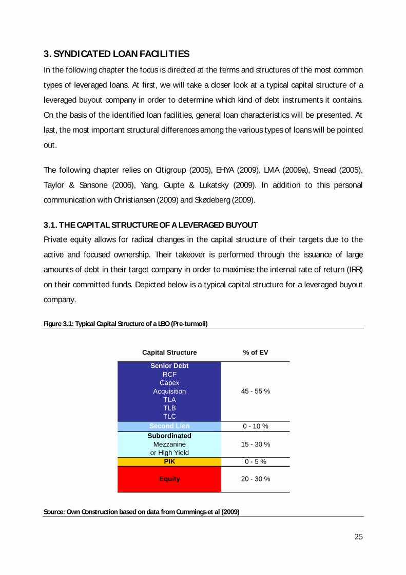
3.1. THE CAPITAL STRUCTURE OF A LEVERAGED BUYOUT

Private equity allows for radical changes in the capital structure of their targets due to the

active and focused ownership. Their takeover is performed through the issuance of large

amounts of debt in their target company in order to maximise the internal rate of return (IRR)

on their committed funds. Depicted below is a typical capital structure for a leveraged buyout

company.

Figure 3.1: Typical Capital Structure of a LBO (Pre-turmoil)

Source: Own Construction based on data from Cummings et al (2009)

Senior DebtRCF

Capex

Equity

Second LienSubordinated

0 - 10 %

15 - 30 %

PIK

Capital Structure

Mezzanineor High Yield

AcquisitionTLATLBTLC

0 - 5 %

20 - 30 %

% of EV

45 - 55 %

26

As seen in figure 3.1, leveraged buyouts tend to have a complex financial structure consisting of

a wide range of different debt products. The capital structure typically involves senior debt,

second lien, and some kind of subordinated debt, such as mezzanine or high yield bonds and

occasionally PIK notes.

3.2. LEVERAGED LOAN CHARACTERISTICS

Based on the illustrated capital structure above, the following section will give an exposition of

the general terms of the most commonly seen leveraged loans.

3.2.1. Coupons - Floating Rate

Leveraged loans are structured with variable interest payments set by a pre-determined spread

above a certain reference rate. In Europe the most frequently used benchmark rates are Libor

and Euribor. To investors, floating rate structures work as a hedge against interest rate changes

whereas borrowers, on the contrary, are exposed to changes in the reference rate. The loan

agreement, typically, dictates the borrower to hedge against interest rate changes as an

extreme vulnerability towards this risk is present.

3.2.2. Tenor - Maturity and Call-ability

Leveraged loans have maturities as short as one to five years for working capital revolvers while

leveraged term loans normally mature in seven to ten years. Typically maturities are: TLA - 7

years, TLB - 8 years, TLC - 9 years, TLD – 10 years, etc. Carrying a floating rate generally makes

the term loans callable at par. This entails that the issuer can repay their loans partially or in

total at any time. Occasionally, some leveraged loans will have embedded non-call periods or

call protection in them, requiring the issuer to pay a penalty premium for an early redemption.

However, investors are exposed to a credit spread call option, since loans are usually callable

immediately. The decision of the company to call will be based on an assessment of whether

the company can access loan funds more cheaply due to improved market conditions,

improvements in the company’s creditworthiness, or if it simply generates excess cash. In

recent years’ pleasant market conditions, it has become increasingly popular to execute a

dividend recap. This implies that the private equity firm withdraws capital and replaces it with

additional debt in connection with a total refinancing.

27

3.2.3. Covenants - Early Warning

One of the most important aspects associated with leveraged loans is the comprehensive

covenant package. Covenants are outlined in the legal credit agreement as series of restrictions

that dictate how borrowers can operate and carry themselves financially. In this way, covenants

limit a borrower’s ability to increase credit risk beyond certain specific parameters. The size of

the covenant package varies according to the borrower’s financial risk at issue. In general, there

are three primary types of loan covenants: (1) Affirmative, (2) Negative, and (3) Financial.

Affirmative covenants state what action the borrower must do to be in compliance with the

loan. Most of these requirements are usually boilerplate such as paying taxes, complying with

laws, and meeting financial obligations. Things the borrower would normally do without being

instructed by a lender. Additionally, almost every credit agreement includes a more

comprehensive disclosure covenant which requires the borrower to deliver annual audited and

monthly unaudited financial statements. In this way, the lenders get the possibility to

continuously monitor the performance of the borrower.

Negative covenants are structured and customised to limit some specific activities of the

borrower according to its conditions. The most common restrictions are within no dividend

payments, cross default, negative pledge, change of control, new investments, indebtedness,

sale of assets, mergers and acquisitions, and guarantees.

Financial covenants are the most comprehensive types of covenants appearing in the loan

agreement. These covenants impose minimum financial performance measures against the

borrower. Covenant tests reveal the credit health of a borrower and allow lenders to take

action in the event a borrower gets into credit trouble. Usually, financial covenants are tested

every quarter. If a covenant is breached the lenders can require the loan to be repaid or agree

to amend the covenant to keep the borrower in compliance with the credit agreement.

A credit agreement for a leveraged loan will typically contain up to four types of financial

covenants depending on the credit risk of the borrower and market conditions at issue. Some

of the most commonly used covenants are:

Debt Coverage: Total debt/EBITDA

Cash Flow Coverage: Cash flow/Net debt service

Interest Coverage: EBITDA/Net finance charges

Maximum CAPEX

28

3.2.4. Security - Lien against Assets and Shares

In general, leveraged loans are structured with a lien against all material assets of the borrower,

which are relatively easy to pawn without being too costly. This usually includes receivables,

inventory and cash, fixed assets and real property. In addition, the loan holders have a lien

against all the shares of the operating company and material subsidiaries. The lien provides a

claim on the control of the company including its assets, and gives secured loan holders several

advantages over unsecured investors. In the event of a default, the secured lenders can take

possession of the assets they claim to and sell or operate them for cash. Although, such a

liquidation option is rarely used in practice, it does put the lender in an excellent position to

maximise the recovery of principal in a restructuring.

3.2.5. Seniority - Corporate and Legal Ranking

As illustrated in figure 3.1 above, private equity owned companies tend to have complex capital

structures containing several different products with different security. In this respect it is of

great importance to ensure the right order of payments - particularly in connection to

underperformance or default. This is usually achieved in two ways: (1) Structural and (2) Legal.

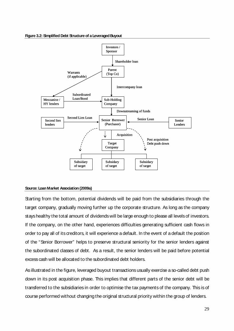
Depictured below, in a schematic drawing of a simplified leveraged debt structure, the private

equity fund typically structures the transaction in accordance with the various investors’

priority.

29

Figure 3.2: Simplified Debt Structure of a Leveraged Buyout

Source: Loan Market Association (2009a)

Starting from the bottom, potential dividends will be paid from the subsidiaries through the

target company, gradually moving further up the corporate structure. As long as the company

stays healthy the total amount of dividends will be large enough to please all levels of investors.

If the company, on the other hand, experiences difficulties generating sufficient cash flows in

order to pay all of its creditors, it will experience a default. In the event of a default the position

of the “Senior Borrower” helps to preserve structural seniority for the senior lenders against

the subordinated classes of debt. As a result, the senior lenders will be paid before potential

excess cash will be allocated to the subordinated debt holders.

As illustrated in the figure, leveraged buyout transactions usually exercise a so-called debt push

down in its post acquisition phase. This implies that different parts of the senior debt will be

transferred to the subsidiaries in order to optimise the tax payments of the company. This is of

course performed without changing the original structural priority within the group of lenders.

Investors / Sponsor

Parent(Top Co)

Sub-HoldingCompany

Senior Borrower(Purchaser)

TargetCompany

Senior Lenders

Subsidaryof target

Subsidaryof target

Mezzanine / HY lenders

Second lien lenders

Subsidaryof target

Senior Loan

Acquisition

Second Lien Loan

SubordinatedLoan/Bond

Warrants (if applicable)

Shareholder loan

Intercompany loan

Downstreaming of funds

Post acquisitionDebt push down

Investors / Sponsor

Parent(Top Co)

Sub-HoldingCompany

Senior Borrower(Purchaser)

TargetCompany

Senior Lenders

Subsidaryof target

Subsidaryof target

Mezzanine / HY lenders

Second lien lenders

Subsidaryof target

Senior Loan

Acquisition

Second Lien Loan

SubordinatedLoan/Bond

Warrants (if applicable)

Shareholder loan

Intercompany loan

Downstreaming of funds

Post acquisitionDebt push down

30

In a legal sense, intercreditor agreements and cross-guarantees, likewise, work to ensure lender

rights. The intercreditor agreement outlines the ranking and specifies the priority of repayment

to all lenders in the case of a default. Cross-guarantees similarly ensure that the varied

operating units associated with a borrower guarantee their shares and assets as collateral.

Thus, should one part trigger a default, all the associated companies will be equally responsible

and their assets will be available for repayment.

3.2.6. Market and Information - Private Market

An important distinction between high yield bonds and leveraged loans is the underlying

information material. Loans are strictly private securities, while high yield bonds are

characterised as public instruments. Syndicated loans are originated and maintained based on

information which often contains material of non-public character. Consequently, syndicate

information shared between the issuer and the lender group is considered to be confidential.

However, it is still possible to preserve the option to trade in the public securities market,

although taking part in the loan market. As earlier mentioned, most arrangers will prepare a

public version of an information memo in which private information, like projections, are

omitted. These memos will be distributed to accounts which request to trade on the basis of

public information. Furthermore, the arrangers will arrange a public version of the subsequent

bank meeting.

One of the main reasons why leveraged buyouts are capable of obtaining such high degrees of

leverage is the comprehensive due diligence material. The private equity fund hires a series of

consultancies to perform different types of due diligences on its target working as a fixture of

the carefully structured purchasing process. This involves exhaustive analyses of private

information which is put at the private equity fund’s disposal. On the basis of these in-depth

analyses, potential investors get a much better understanding of the underlying business of the

firm. This entails that lenders confidence in investing in the companies increase. On the

contrary, the high yield bond investors have to be content with the public material available.

This, of course, results in a much higher degree of uncertainty with respect to the insight of the

performance of the company. Consequently, the due diligence process equips the investors in

the private loan market with much better possibilities to predict how well the specific company

will perform in the future. In general, this allows for a higher amount of leveraged compared to

what investors typically are willing to accept.

31

3.3. LEVERAGED LOANS VERSUS HIGH YIELD BONDS

Although high yield bonds are not a product launched in the syndicated loan market, these are

similar to leveraged loans in many ways, most importantly, they are both frequently used debt

instruments in leveraged buyout transactions. However, despite their similarities, leveraged

loans and high yield bonds do differ in several notable aspects regarding general terms and

structures.

Leveraged loans carry floating interest rates with spreads quoted over a pre-determined

reference rate, unlike traditional high yield bonds which often have fixed coupon payments.

Setting interest payments as a floating rate coupon offers the investors an effectively built-in

hedge against rising interest rates. Comparison of leveraged loans to high yield bonds also

involves a trade-off between seniority and call-ability. The maturities of leveraged loans are

typically seven to ten years, but due to the floating rate structure they are callable at any time.

High yield bonds generally have longer maturities, on average 10 years, but on the other hand

with investor friendly non-call provisions - typically the first five years. To offset this structural

advantage, leveraged loans offer a senior secured position in the capital structure with more

restrictive financial covenants (often bonds do not even have any). Consequently, defaulted

secured loans consistently exhibit higher recovery rates than unsecured high yield bonds when

utilised in the same transaction. However, nothing comes for free and the reduced risk inherent

in the senior secured status results in a lower yield. A final notable difference is the information

gap. Most leveraged loan investors enjoy access to more complete information due to the fact

that they are traded on the basis of private information. High yield bond investors, on the other

hand, must rely on the public information available.

To sum up, leveraged loans have evolved to be the fixed income asset class receiving the most

investor attention. This is primarily due to their distinct features which neatly addresses two of

the primary risks in fixed income investing: (1) Floating rate coupons help to mitigate interest

rate risk, and (2) Protective covenants and senior position help mitigate credit risk. As a result,

recent years’ total new issuance of leveraged loans has by far outpaced the new issuance of

public high yield bonds (EHYA, 2009).

32

3.4. STRUCTURES OF LEVERAGED LOANS

Moving on from the general terms of leveraged loans, the following part of the paper

distinguishes between the individual loan types, providing a fundamental understanding of the

specific loan structures. Understanding the basics of how the different loans work in practise is

simply necessary from a potential investor’s point of view.

3.4.1. Structure of a Revolving Credit Line

The revolving credit facility constitute a maximum aggregate amount of unfunded or partially

funded commitments which can be drawn, repaid and re-drawn at the borrowers discretion

until maturity. The structure of the facility resembles that of a credit card, with the exception

that borrowers are charged an additional non-use facility fee on unused amounts. Revolving

credit lines generally serve as liquidity facilities to fund working capital or capital expenditures.

Maturities are in general either one year or in the range of three to five years. From an investor

perspective revolvers are complicated to administer and fund due to the uncertain funding

requirements and interest payments. Consequently, these loans are held almost entirely by

traditional banks.

3.4.2. Structure of a First Lien Term Loan - Amortising and Institutional

In compliance with the demand of the two primary syndicated lender constituencies - banks

and institutional investors – first lien loans are structured as either: (1) Amortising debt or (2)

Institutional debt.

Amortising TLAs are typically structured as fully funded term loans with progressive repayment

schedules running seven years or less. As the principal gets repaid, the borrower is unable to re-

borrow the money, thereby differentiating them from the revolving credit facility. TLAs are

primarily structured to be committed by traditional banks, due to the nature of accelerated

amortisation payments. However, in some syndicated agreements, institutional investors have

made commitments to the term loan A as a way to secure a larger portion of the institutional

tranches.

In order to comply with the increased institutional investor demand, the structures of an

increasing number of deals have been adjusted by entirely excluding the term loan A in favour

of institutional tranches.

33

Most of the institutional debt consists of the first lien term loan facilities TLB and TLC. These

tranches are jointly referred to as TLBs, because of their bullet payments and the fact that they

are lined up behind TLAs. Institutional term loans possess a variety of structural differences

compared to their less-liquid amortising counterparts. As the name implies, the tranches are

structured primarily to favour the rising number of institutional investors in the form of more

predictable funding requirements and interest payments. Maturities are, in general, gradually

increasing, e.g. term loan B might be eight years, term loan C nine years, term loan D ten years,

etc. These loans are priced higher than amortising term loans, because of the longer maturities

and bullet repayment schedules. Leveraged loan investors usually expect to receive an

additional 25 bps – 75 bps in coupon for each additional year until maturity. In practice,

however, spreads of course reflect what the market is demanding in compensation for longer

maturities.

3.4.3. Structure of a Second Lien Term Loan

Second lien has, since its entrance in the European loan market in 2004, joined the ranks of

mezzanine as a financing alternative in private equity transactions. Second lien is a bi-product

of the hyper-liquid market conditions of recent years’. It is a debt instrument used as an

extension of the senior part of the capital structure on behalf of the more expensive

subordinated debt. Consequently, second lien has always been more popular among borrowers

than lenders. However, in years with plenty of liquidity, the utilisation of second lien has

steadily grown. In fact, in the days preceding the credit crisis it became almost an intrinsic part

of LBO financing.

Generally seen, second lien loans are structured much like the more common institutional first

lien loans. They are typically: (1) Fully drawn, with (2) bullet maturities (3) floating rate coupons

(4) secured lien on the assets of the borrower, and (5) share the same covenant package as first

lien facilities. Although, second lien loans are really just another type of syndicated loan facility,

they are rather more complex. The following points show the primary characteristics that set

second lien term loans apart from the more liquid first liens:

34

As the name implies a second lien on asset collateral of the borrower. First lien lenders

are entitled to be paid in full before any distributions are made to second lien holders

Larger coupons due to the higher risk

Longer maturity, usually set a year after the first lien maturity date

A waiver of certain rights in case of bankruptcy to the first lien lenders which are

spelled out in the legal intercreditor agreement. E.g. first lien holders have the right to

decide on disposition of shared collateral, including asset sales and bankruptcy exit

financing.

3.4.4. Structure of a Mezzanine Loan

A mezzanine loan is a subordinated debt instrument that carries second-ranking security, or

third-ranking security, if the capital structure includes second lien. Mezzanine fills the gap

between senior debt and equity in the capital structure and is often referred to as "in between"

debt. Mezzanine loans are typically used as an alternative to high yield bonds when companies

do not have enough assets or current cash flow to qualify for additionally senior debt. Instead

of lining up additional equity mezzanine debt serves to stretch out the total debt structure.

Investors may be rewarded with yield enhancements such as warrants since mezzanine debt

contains higher risk than senior secured loans. By incorporating “equity kickers” lenders are

given a stake in the company’s upside potential.

Historically, mezzanine has been an option for smaller transactions while the high yield bond

market provided the subordinated financing for larger deals. Mezzanine debt was primarily a

funding option when the financial needs were too small to qualify for the high yield bond

market. However, mezzanine has in the past few years extended its reach to include larger

deals, due to the hyper-liquid conditions in the leveraged loan market. Actually mezzanine has

become a staple of LBO financings because of its relatively strong position in the subordinated

part of the capital structure and its strong covenants2. Furthermore, mezzanine loans have

shorter non-call provision - typically one to three years - plus prepayment penalties at 102 bps

and 101 bps in the subsequent years. This appeal to private equity funds with respect to exiting

their targets. In these situations it will be cheaper to repay mezzanine than high yield bonds

which generally have longer non-call periods embedded.

2 Mezzanine typically carries the same financial covenants as senior bank loans though some facilities include a haircut on the covenants. Usually the looser level is around 10 %, placing the headroom in the 30 – 35 % area.

35

3.4.5. Structure of a Payment-in-kind Loan

Payment-in-kind loans (PIK) are debt instruments that pay investors in the form of additional

principal rather than cash coupons. Like zero-coupon bonds, they give a company breathing

space before having to make cash outlays at maturity. PIK loans are primarily utilised when the

purchase price of the target exceeds leverage levels, up to which lenders are willing to provide

additional senior, second lien, or mezzanine loans. As a result, PIK loans rank last in the capital

structure and are used as a final substitute for equity. However, with the rich yields offered by

PIK loans, the private equity fund has to be very diligent in assessing whether the cost of

incorporating PIK loans does not outbalance the IRR on its equity investment.

3.5. PRICING STANDARDS

For many years, European loan prices were not very flexible and market-driven. The loan

market had a well-established pricing standard from where most deals started out. The

revolving credit facilities and TLAs usually began at a base rate (BR) + 225 bps, whereas each of

the following institutional tranches were added an additional 50 bps - pricing TLB at BR + 275

bps and TLC at BR + 325 bps etc. While the pricing of the most senior tranches for many years

were relatively fixed, the spreads of the more optional loans, such as second lien and

mezzanine, have varied more widely. Second lien loans have usually been priced in the BR + 500

bps area, depending on the complexity and riskiness of the underlying credit. In the same way,

the subordination of the mezzanine loans make the margin considerably higher than on senior

loans - ranging anywhere from BR + 700 bps to BR + 1.100 bps. In addition to spread premiums,

mezzanine debt may have warrants included to provide lenders an unlimited upside potential,

should the issuer perform well. Deals with warrants of course carry lower spreads than those

without.

Market flex pricing has become more standard in Europe, thanks to the increased institutional

investor base. As previously mentioned, margin flex pricing allows the arranger to change

spreads during syndication to adjust pricing to current liquidity levels. Consequently, in the

years prior to the liquidity crunch, the vast majority of deals opened at prices slightly below

older standards. In this period, borrowers profited from the hyper-liquid market conditions

reducing the price levels on the senior tranches to BR + 200/250/300 bps. However, once the

36

financial crisis accelerated the opening spread levels went up and exceeded the old standards

by far.

Although market-flex structure has become standard, pricing of leveraged loans is not yet fully

driven by capital market forces. Contrary to the U.S., the European leveraged loan market is still

affected by banks remaining a dominant market player. In the U.S., the pricing is exclusively

determined by the predominant institutional investor appetite.

3.6. CHAPTER SUMMARY

The leveraged loan market consists of loans made for speculative grade borrowers. The vast

majority of loans are senior secured floating rate papers which the issuer can prepay with little

or no restrictions or fees. The senior loans are either denoted as first lien or second lien which

reflects their security ranking in the capital structure and, thus, their claims on collateral. In

addition, mezzanine loans have become an increasingly used LBO financing tool within the

subordinated debt ranking. Due to the high credit risk incorporated in leveraged loans, the

issuers are restricted by comprehensive covenant packages which state how loose they can

operate and carry themselves financially. In addition, the various loan types are structured with

different maturities, repayment schedules and pricing standards. All of which are summed up in

table 3.3.

37

Table 3.3: General Terms of Debt Instruments Utilised in a Leveraged Buyout


Senior Second Lien Mezzanine High Yield PIK Notes

Coupon Floating rate Floating rate Floating rate Fixed/Floating rate Fixed/Floating rate

Tenor • Usually 7, 8, 9 years for TLA, TLB, TLC respectively • Pre-payable without penalty • Repayable on change of control

• 9.5 years• Typically pre-payable without penalty• Repayable onchange of control

• 10 years• No-call provision for one to three years, plus pre-payment penalties at 102, 101 in the subsequent years• Repayable on changeof control

• Typ ically 10-year• Not usually pre-payable for 5years• Penalty of ½ coupon afteryear 5, diminishing thereafterto zero• 101 put on change of control

• 11 years• Non-call protection, generally in first 3 - 4 years

Covenants Broad range of financial and non-financial maintenance covenants. Headroom typically 20 – 25%

Same package ofcovenants as senior.Headroomtypically 20 – 25%

Similar package ofcovenants to seniorbut headroomusually 10% higher

Incurrence covenants only Incurrencesame as HYbut set onelevel higher

Security Enjoys first pledge over all major subsidiaries through combination of structural / contractual subordination

Shares securitywith Senior;however, issecond in line forrepayment

Second/third (ifstructure has secondlien)

None or second lien (subordinated)

None

Seniority 1st ranking Ranks equal toSenior but aboveMezzanine andHigh Yield

Ranks behind Seniorand 2L but aboveany High Yield

Behind senior,2L, Mezzanine

Ranks last

Repayments • TLA amortizising • Other tranches bullet repayments

Bullet Bullet Bullet Bullet

Market/Information

• Private market • Information mostly private

• Private market• Information mostly private

• Private market• Information mostly private

• Public market• Public information

Public or Private

Spread BR + 225 bps starting from term loan A adding an additionally 50 bps for each of the following tranches

BR + 500 bps • A hybrid product often consisting yield enhancements such as warrants and PIKs. • Total margin ranging anywhere from BR + 700 bps to BR + 1100 bps

7,5 - 12 % 8 - 15 %

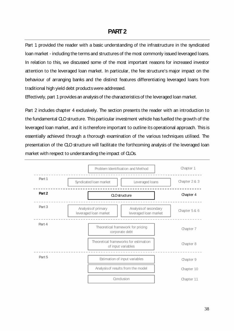
38

PART 2

Part 1 provided the reader with a basic understanding of the infrastructure in the syndicated

loan market - including the terms and structures of the most commonly issued leveraged loans.

In relation to this, we discussed some of the most important reasons for increased investor

attention to the leveraged loan market. In particular, the fee structure’s major impact on the

behaviour of arranging banks and the distinct features differentiating leveraged loans from

traditional high yield debt products were addressed.

Effectively, part 1 provides an analysis of the characteristics of the leveraged loan market.

Part 2 includes chapter 4 exclusively. The section presents the reader with an introduction to

the fundamental CLO structure. This particular investment vehicle has fuelled the growth of the

leveraged loan market, and it is therefore important to outline its operational approach. This is

essentially achieved through a thorough examination of the various techniques utilised. The

presentation of the CLO structure will facilitate the forthcoming analysis of the leveraged loan

market with respect to understanding the impact of CLOs.

CLO structure






Part 2

Part 3

Chapter 2 & 3

Chapter 5 & 6

Chapter 7

Chapter 1

Chapter 9

Chapter 8

Chapter 4




Conclusion

Chapter 10

Chapter 11

Part 4

Part 5

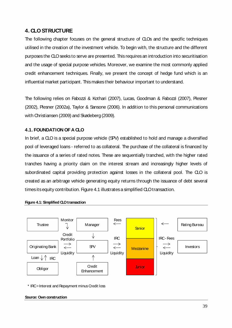
39

4. CLO STRUCTURE

The following chapter focuses on the general structure of CLOs and the specific techniques

utilised in the creation of the investment vehicle. To begin with, the structure and the different

purposes the CLO seeks to serve are presented. This requires an introduction into securitisation

and the usage of special purpose vehicles. Moreover, we examine the most commonly applied

credit enhancement techniques. Finally, we present the concept of hedge fund which is an

influential market participant. This makes their behaviour important to understand.

The following relies on Fabozzi & Kothari (2007), Lucas, Goodman & Fabozzi (2007), Plesner

(2002), Plesner (2002a), Taylor & Sansone (2006). In addition to this personal communications

with Christiansen (2009) and Skødeberg (2009).

4.1. FOUNDATION OF A CLO

In brief, a CLO is a special purpose vehicle (SPV) established to hold and manage a diversified

pool of leveraged loans - referred to as collateral. The purchase of the collateral is financed by

the issuance of a series of rated notes. These are sequentially tranched, with the higher rated

tranches having a priority claim on the interest stream and increasingly higher levels of

subordinated capital providing protection against losses in the collateral pool. The CLO is

created as an arbitrage vehicle generating equity returns through the issuance of debt several

times its equity contribution. Figure 4.1 illustrates a simplified CLO transaction.

Figure 4.1: Simplified CLO transaction

Source: Own construction

Trustee

Originating Bank

ObligorCredit

Enhancement

SPV

Manager

Investors

Rating BureauSenior

Mezzanine

Junior

Liquidity LiquidityLiquidity

Credit Portfolio

Monitor

Loan

* IRC = Interest and Repayment minus Credit loss

IRC

IRC IRC - Fees

Fees

40

The creation of a SPV plays a key role in the creation of a CLO as it enables asset based

structuring to be applied to leveraged loans. The concept of securitisation concerns the

issuance of securities with a direct connection to specific assets. In relation to CLOs,

securitisation can be described as the process in which banks pool together the interests from

leveraged loans in identifiable future cash flows. A SPV is created to which the claims on the

future cash flows are transferred. The SPV serves the sole purpose of holding these financial

claims and utilise the future cash flows to pay off investors over time. In fulfilling the role as

originators, banks are effectively provided funding by selling a stream of cash flows that would

otherwise be accrued to them. The originating bank which initially committed the loans,

thereby obtains ongoing servicing fees associated with the transfer of interest payments -

without burdening the capital adequacy requirements. In applying securitisation the originator

is not affected by any risks associated with the underlying pool of assets, as it only distributes

the cash flows generated by these.

Similarly, investors are not affected by any risks associated with the originator following the

creation of the SPV as an independent legal entity. In order to obtain bankruptcy remoteness

the interests of the investors must be safeguarded by a trustee in economical arms-length to

the originator.

Effectively, banks achieve off-balance financing whereby regulatory capital restraints no longer

limit their loan issuance. Simultaneously, they benefit from servicing the cash flows and

maintaining the role as corporate relationship banks.

Before turning to the exposition of credit enhancement techniques the next section will outline

the main reasons for the structuring of the investment vehicle.

4.2. PURPOSE OF THE CLO

The CLO concept was initially introduced with the purpose of providing banks regulatory capital

relief. The creation of the balance sheet CLO facilitated banks in selling portions of their loan

portfolio in the capital markets. According to Plesner (2002), banks rather easily disposed of the

senior and mezzanine tranches, while they were often forced to retain the junior tranche due

to its highly incorporated credit risk. As a consequence, the junior tranche was often referred to

as equity.

41

The retention of the equity tranche soon resulted in banks issuing arbitrage CLOs in favour of

the traditional balance sheet CLO. The investment objective of the new arbitrage CLO structure

was to maximise excess spread, hence creating an arbitrage from the perspective of the equity

investors3. To achieve the desired excess spread on the equity tranche an optimisation of the

capital structure became crucial which lead to an increased extent of applied credit

enhancement. In outline credit enhancement refers to various techniques applied to mitigate

risk with respect to expected as well as unexpected losses in the collateral pool. This allowed

for more tranches in the capital structure to comply with different investor requirements and

more leverage was obtained. In this way, a minimisation of total liability payments was

achieved and returns on the reduced equity tranche increased to a degree which actually made

the tranche desirable for investors.

The above mentioned structural shift from balance sheet to cash flow arbitrage highly

increased the complexity of the CLO structure due to the credit enhancement and increased

number of tranches. This complex structure was later criticised by loan market investors

claiming that banks had forced the loans into the market. The accusations primarily concerned

that banks had only been motivated by maximisation of their associated fees which gradually

increased along with the complexity of the CLO structure. It is, however, worth remembering

that the banks were only capable of selling what investors demanded. With the CLO structure

enabling subordination of debt - resulting in tranches with different interest rates and credit

ratings - different types of investor needs were addressed. In fact, the applied credit

enhancement, which enabled investment-grade ratings to be obtained, was highly desirable to

institutional investors due to the solvency burden associated with the lower rated leveraged

loans.

In addition, institutional investors do not have departments specialised in the leverage loan

business since leveraged loans only constitute a minor part of their total portfolio. Their limited

expertise within the area is another important reason for institutional investors’ considerable

utilisation of CLOs. Investing directly in leveraged loans is a complicated and time consuming

process which previously kept institutional investors out of the market. With the entrance of

CLOs a golden opportunity to invest in diversified portfolios of leveraged loans arose. In this

3 For a numerical illustration of how excess spread is achieved see appendix A.

42

way, CLOs heavily impacted the rapidly increasing institutional investor base in the leveraged

loan market.

To sum up, the CLO structure has provided banks the opportunity to achieve off-balance sheet

financing while simultaneously generating fees from servicing the loans and remaining the

corporate relationship bank. This highly motivated banks to apply asset based structuring as

oppose to selling the loans directly to the investors. Likewise, the CLO structure has provided

Institutional investors with a variety of opportunities to invest in leveraged loans with

investment-grade ratings.

With the general purposes of the CLO in place, an introduction to how credit enhancement

techniques allows for the fulfilment of these succeeds.

4.3. CREDIT ENHANCEMENT TECHNIQUES

Credit enhancement refers to the actions taken in order to mitigate the risk associated with

default in the collateral pool. Credit enhancement is performed to achieve a certain target

rating for the specific notes which implies different levels of enhancement for each class of

securities. The three most commonly applied techniques are those of: (1) Excess spread, (2)

Subordination, and (3) Overcollateralisation. While excess spread covers expected losses,

unexpected losses are addressed by subordination and overcollateralisation.

Excess spread is generated when the weighted average rate of interest on the collateral is

greater than the weighted average rate of interest on the liabilities. It is commonly known that

lenders will charge a risk premium for credit risk which in the context of the CLO is the expected

losses on the collateral pool. Excess spread is achieved to absorb the potential expected losses

from the collateral pool. With senior note holders protected by the tranche with the lowest

priority they are not exposed to the expected losses. This implies that the entire risk of the

collateral pool is diverted to the most junior tranche, but so is the entire risk premium.

Subordination refers to the order of priority in the sequentially tranched notes. The most junior

tranche is the first to suffer losses exceeding excess spread, and then moving upwards in the

capital structure. With any tranche protected by subordinated debt, a higher credit rating than

the actual collateral pool is achievable.

Overcollateralisation creates protection to investors by over-collateralizing the liabilities. The

over-collateralized assets thereby become a subordinated share of the seller which is available

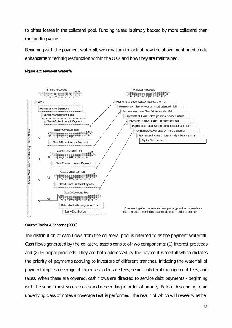
43

to offset losses in the collateral pool. Funding raised is simply backed by more collateral than

the funding value.

Beginning with the payment waterfall, we now turn to look at how the above mentioned credit

enhancement techniques function within the CLO, and how they are maintained.

Figure 4.2: Payment Waterfall

Source: Taylor & Sansone (2006)

The distribution of cash flows from the collateral pool is referred to as the payment waterfall.

Cash flows generated by the collateral assets consist of two components: (1) Interest proceeds

and (2) Principal proceeds. They are both addressed by the payment waterfall which dictates

the priority of payments accruing to investors of different tranches. Initiating the waterfall of

payment implies coverage of expenses to trustee fees, senior collateral management fees, and

taxes. When these are covered, cash flows are directed to service debt payments - beginning

with the senior most secure notes and descending in order of priority. Before descending to an

underlying class of notes a coverage test is performed. The result of which will reveal whether

Equity Distribution

Subordinated Management Fess

Class D Note Interest Payment

Class C Note Interest Payment

Class B Note Interest Payment

Class A Note Interest Payment

Senior Management Fees

Administrative Expences

Class A Coverage Test

Class D Coverage Test

Class C Coverage Test

Class B Coverage Test

Interest Proceeds Principal Proceeds

Taxes Payments to cover Class A Interest shortfall

Payments of Class A Note principal balance in full*

Payments to cover Class B Interest shortfall

Payments of Class B Note principal balance in full*

Payments to cover Class C Interest shortfall

Payments of Class C Note principal balance in full*

Payments to cover Class D Interest shortfall

Payments of Class D Note principal balance in full*

Equity Distribution

Rede

em M

ost

Seni

or O

urst

andi

ng C

lass

of N

otes

Fail

Fail

Fail

Fail

Pass

Pass

Pass

Pass

* Commencing after the reinvestment period, principal proceeds are paid to reduce the principal balance of notes in order of priority

44

the collateral is performing within the rules set forth in the prospectus. Should the collateral

value or cash flows be insufficient to pass a coverage test, distributions to investors below this

point is terminated and diverted to redeem the most senior class of notes. Cash flows are

continuously diverted until the test can be passed and, as such, the CLO structure is

deleveraging as a self-correcting mechanism. This implies that any deterioration in the cash

flows generated from the collateral will affect investors of the lowest prioritised tranche first. In

addition, subordinated management fees are relinquished when failures to meet coverage tests

occur in the capital structure.

The indenture, formulated upon the creation of the CLO, contains two types of covenants to

protect note holders and maintain credit ratings on the notes. These are (1) Collateral coverage

tests and (2) Portfolio quality tests.

Collateral coverage tests are designed to protect note holders against deterioration in the

existing portfolio. This is performed to maintain the required minimum levels of credit

enhancement and excess spread assigned to the specific ratings of the individual notes.

To ensure the credit enhancement whereby minimum asset coverage is achieved, an

overcollateralisation test must be performed. The O/C test makes certain that each debt

tranche is protected by a minimum level of par value asset coverage. The O/C ratio for a

tranche is found by solving the following

푂/퐶 푟푎푡푖표 =푃푎푟 푣푎푙푢푒 표푓 푐표푙푙푎푡푒푟푎푙 푝표푟푡푓표푙푖표

(푃푎푟 푣푎푙푢푒 표푓 푡푟푎푛푐ℎ푒 + 푝푎푟 푣푎푙푢푒 표푓 푎푙푙 푡푟푎푛푐ℎ푒푠 푠푒푛푖표푟 푡표 푖푡)

The higher the ratio, the greater the protection to note holders. When performing the test the

O/C ratio must be equal to or greater than the required minimum ratio which is referred to as

the O/C trigger.

The excess spread is protected by an interest coverage test performed to ensure that adequate

interest proceeds are available to pay interest due on the notes. The I/C ratio for a tranche is

found by solving

45

퐼/퐶 푟푎푡푖표 =(퐶표푙푙푎푡푒푟푎푙 푐표푢푝표푛 − 푠푒푛푖표푟 푓푒푒푠 푎푛푑 푒푥푝푒푛푐푒푠)

(푆푝푒푐푖푓푖푐 푡푟푎푛푐ℎ푒 푐표푢푝표푛 + 푐표푢푝표푛푠 푓푟표푚 푎푙푙 푡푟푎푛푐ℎ푒푠 푠푒푛푖표푟 푡표 푖푡)

Once again, the higher the ratio the greater the protection is to the note holders. The interest

coverage test for a tranche is passed if the I/C ratio is equal to or greater than the I/C trigger,

which is the required minimum interest coverage ratio as specified in the indenture. If any of

the above coverage tests are failed, actions are as described in the payment waterfall.

Quality tests are designed to ensure that certain criteria of the collateral pool are maintained

on an ongoing basis. They are effectively investment restrictions assigned to maintain the initial

credit rating of the specific note and therefore protect against deterioration in the credit

quality of the portfolio. In general, asset quality tests constitute several individual tests, such as

the minimum average credit rating test. This ensures that the weighted average rating of the

collateral pool is at or above a specified level. Furthermore, tests for minimum levels of

portfolio diversification typically limit the maximum percentage of collateral assets in the same

industry or issued by the same obligor. Finally, quality tests only allow for a specific maximum

amount of CCC-rated investments in the portfolio - often referred to as the CCC bucket.

Quality tests are typically described as maintain or improve tests - referring to how they merely

restrict trading. Failure of meeting the requirement in a quality test will usually just result in

subsequent trades being restricted to actions improving the collateral pool relative to the

breached test. In contrast to coverage tests, quality tests do not directly influence the priority

of the payment waterfall. However, failure to comply with the restrictions in a test can

indirectly affect the waterfall by triggering a coverage test to fail as illustrated in the example

below.

The CCC bucket in a CLO typically allows for a maximum of 5 – 7.5 percent CCC-rated assets.

Any excess share of CCC rated assets will be mark-to-market which will inevitably influence the

overcollateralisation test. Figure 4.3 illustrates how the overcollateralisation test is affected

when the maximum level of the CCC bucket is breached.

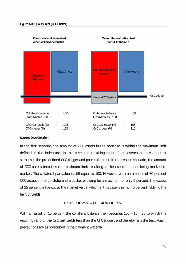
46

Figure 4.3: Quality Test (CCC Bucket)

Source: Own Creation

In the first scenario, the amount of CCC assets in the portfolio is within the maximum limit

defined in the indenture. In this case, the resulting ratio of the overcollateralisation test

surpasses the pre-defined O/C trigger and passes the test. In the second scenario, the amount

of CCC assets breaches the maximum limit resulting in the excess amount being marked to

market. The collateral par value is still equal to 100. However, with an amount of 30 percent

CCC assets in the portfolio and a bucket allowing for a maximum of only 5 percent, the excess

of 25 percent is haircut at the market value, which in this case is set at 40 percent. Solving the

haircut yields

퐻푎푖푟푐푢푡 = 25% ∗ (1− 40%) = 15%

With a haircut of 15 percent the collateral balance then becomes 100 – 15 = 85 to which the

resulting ratio of the O/C test yields less than the O/C trigger, and thereby fails the test. Again,

precautions are as prescribed in the payment waterfall.

Collateral balance

Class A note

O/C trigger

Haircut collateral balance

Class A note

Excess CCC assets

Overcollateralization testwhen within the bucket

Overcollateralization testwith CCC haircut

Collateral balance 100Class A notes / 80--------------------------------O/C test result (%) 125O/C trigger (%) 115

Collateral balance 85Class A notes / 80--------------------------------O/C test result (%) 106O/C trigger (%) 115

47

In recent years, a new CLO structure has entered the market. The market value CLO resembles

the above mentioned cash flow CLO in waterfall structure and ability to leverage the returns of

the collateral. The separating point is the reliance on the market value of the portfolio to serve

as protection for the debt holders. Where the traditional cash flow CLO structure depends on

compliance with covenants concerning default rates and credit quality, the market value CLO

have covenants restricting the minimum value of the collateral pool.

The market value of the collateral is “haircut” by assigning a pre-determined rate to the

underlying collateral. The value of the haircut must be equal to or greater than the amount of

debt. For example, if the haircut applied is 20 percent, the collateral is “haircut” by 1 – 0.2 =

0.8. This implies that the market value must exceed 80 percent of the total value of debt.

Should this criterion be violated, debt must be partially repaid in order to eliminate the

deficiency, or in the worst case, fully liquidated.

For the market value CLOs and the cash flow CLOs, the issued notes are usually structured with

a twelve to fifteen year maturity - although their life span is expected to be shorter. In general,

a reinvestment period is incorporated during the first three to six years. In this period principal

repayments on investments or proceeds from collateral sales are reinvested in new eligible

collateral. When the reinvestment period has expired principal repayments on investments are

applied to amortise the CLO note obligations, beginning with the most senior tranches and

working down the capital structure. Equity investors will be distributed any principal proceeds

only when all the notes have been repaid.

With an insight into how the CLO is structured and operates we are now able to identify the

characteristics of the loan asset class which has made it ideally suited for securitisation before

the onset of the credit crunch. These characteristics include:

Par value erosion of the collateral pool in the event default has been very limited.

Loan prices exhibited a profound stability enabling them to be reinvested at or near par

in the event of early prepayment - thus avoiding collateral deterioration if only premium

priced new collateral was available.

The matching of floating-rate assets with floating-rate liabilities highly limits the

exposure to interest rate risk.

48

Returns on the loan asset class displayed low correlation with returns on practically any

other asset class which created considerable diversification opportunities to aggregate

investment portfolios.

Finally, liquidity in the loan market progressively improved concurrently with the

initiation of new CLOs, thereby creating a self-enforcing mechanism.

While leveraged loans have drawn the attention of CLOs, other structured vehicles have also

taken the opportunity to invest in this asset class. In this leveraged loan market the most

influential investment vehicle - next to the CLO - is the hedge fund. In the following, we will

briefly introduce the methods utilised by hedge funds when investing in the leveraged loan

market.

4.4. HEDGE FUNDS

Hedge funds involvement in the leverage loan market is attributable to bank loan total return

swaps. Total return swaps (TRS) are derivative products offered by banks, allowing loan market

participants to finance most types of bank loans including leveraged loans. Hedge funds use the

TRS as a tool to obtain their desired leverage. In addition, they avoid the operational aspects of

investing in bank loans.

Basically a bank loan TRS is a contract between two parties to exchange the return on a debt

security for payments of a reference rate + spread. The funding bank purchases the bank loan

and holds it directly on its balance sheet or places it in a special purpose entity. The hedge fund

will then pay swap collateral to the funding bank - also known as the “haircut”. The funding

bank returns the haircut to the hedge fund when both parties have satisfied all of their

obligations under the TRS. If the hedge fund fails to make any required payments under the TRS

the funding bank is allowed to terminate all the swaps. In this respect, the haircut works as a

safeguard to recover any amounts owed to the funding bank. The size of the haircut differs

greatly, but the underlying methodologies for TRS usage are generally the same as presented in

figure 4.4.

49

Figure 4.4: Bank Loan Total Return Swap

Source: Taylor & Sansone (2006)

In a simplified TRS transaction the funding bank of a 10.000.000 principal bank loan requires

collateral in the amount of 1.000.000 equivalent of a 10 percent haircut. This implies that the

hedge fund obtains 10 times leverage. The funding bank pays the hedge fund interest and

potential fees received on the initial bank loan. In return the hedge fund pays a reference rate

plus a spread which is calculated on the purchase cost of the bank loan. The bank loan spread

exceeds the swap financing spread and provides the hedge fund with a positive net interest

under the swap. This is, of course, only true so long as the bank loan is paying interest. The

funding bank earns a net spread over its funding cost by simply passing through all interest and

fees paid on the bank loan. This consists of the difference between the swap funding cost and

its own funding cost of the loan.

The funding bank will pay the realised capital gains to the hedge fund, at the time the loan is

sold or repaid. Realised losses, on the contrary, will be paid by the counterparty to the funding

bank. Consequently, realised appreciation or depreciation can be highly influential on the total

returns effectively obtained by the hedge fund.

Since TRS’ are mark-to market products it is an important requirement that daily market prices

for the underlying loans can be obtained. This feature makes syndicated leveraged loans -

where secondary market pricing is widely available - some of the most suitable bank loans to

finance through TRS’.

Bank Loan

Bank Loan Interest and Fees

Reference Rate + Spread

Interest and Fees

Haircut

Funding Bank Hedge Fund

50


To achieve off-balance financing, banks have provided institutional investors various

investment vehicles which allowed them to enter the leverage loan market. These investment

vehicles primarily constitute cash flow and market value CLOs along with hedge funds. The

CLOs are structured around a payment waterfall which insures that interest and principal

repayments occur in compliance with the priority of the different debt holders. To protect the

debt holders, the cash flow CLO structure relies on default rates and credit quality of the

underlying collateral. Market value CLOs and hedge funds on the other hand, depend on the

market value of the underlying assets to serve as protection. Preceding the credit crisis, several

characteristics of leveraged loans made them ideal investment objectives for institutional

investment vehicles. Especially with respect to securitisation which allowed banks to transfer

the credit risk of the financial assets to loan market investors. Simultaneously, they maintained

the role as relationship bank. In turn, the loan market investors circumvented the risk to the

originator due to the utilisation of a bankruptcy remote SPV.

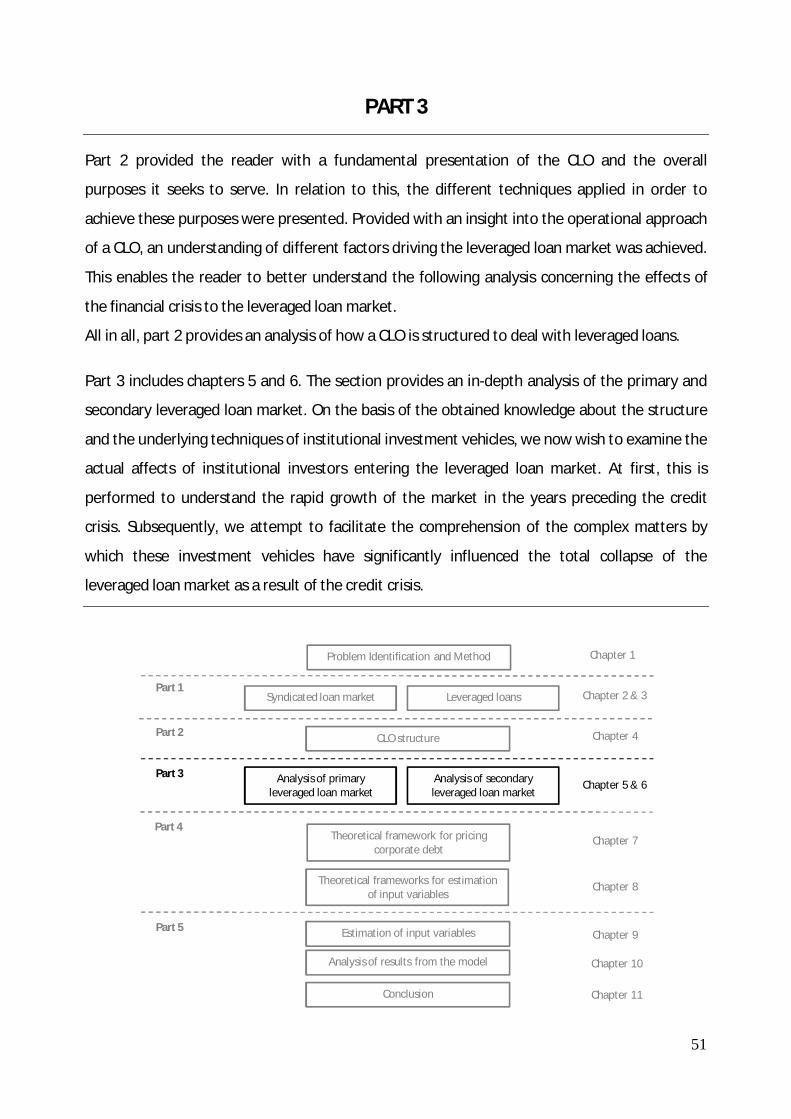
51

PART 3

Part 2 provided the reader with a fundamental presentation of the CLO and the overall

purposes it seeks to serve. In relation to this, the different techniques applied in order to

achieve these purposes were presented. Provided with an insight into the operational approach

of a CLO, an understanding of different factors driving the leveraged loan market was achieved.

This enables the reader to better understand the following analysis concerning the effects of

the financial crisis to the leveraged loan market.

All in all, part 2 provides an analysis of how a CLO is structured to deal with leveraged loans.

Part 3 includes chapters 5 and 6. The section provides an in-depth analysis of the primary and

secondary leveraged loan market. On the basis of the obtained knowledge about the structure

and the underlying techniques of institutional investment vehicles, we now wish to examine the

actual affects of institutional investors entering the leveraged loan market. At first, this is

performed to understand the rapid growth of the market in the years preceding the credit

crisis. Subsequently, we attempt to facilitate the comprehension of the complex matters by

which these investment vehicles have significantly influenced the total collapse of the

leveraged loan market as a result of the credit crisis.

CLO structure






Part 2

Part 3

Chapter 2 & 3

Chapter 5 & 6

Chapter 7

Chapter 1

Chapter 9

Chapter 8

Chapter 4




Conclusion

Chapter 10

Chapter 11

Part 4

Part 5

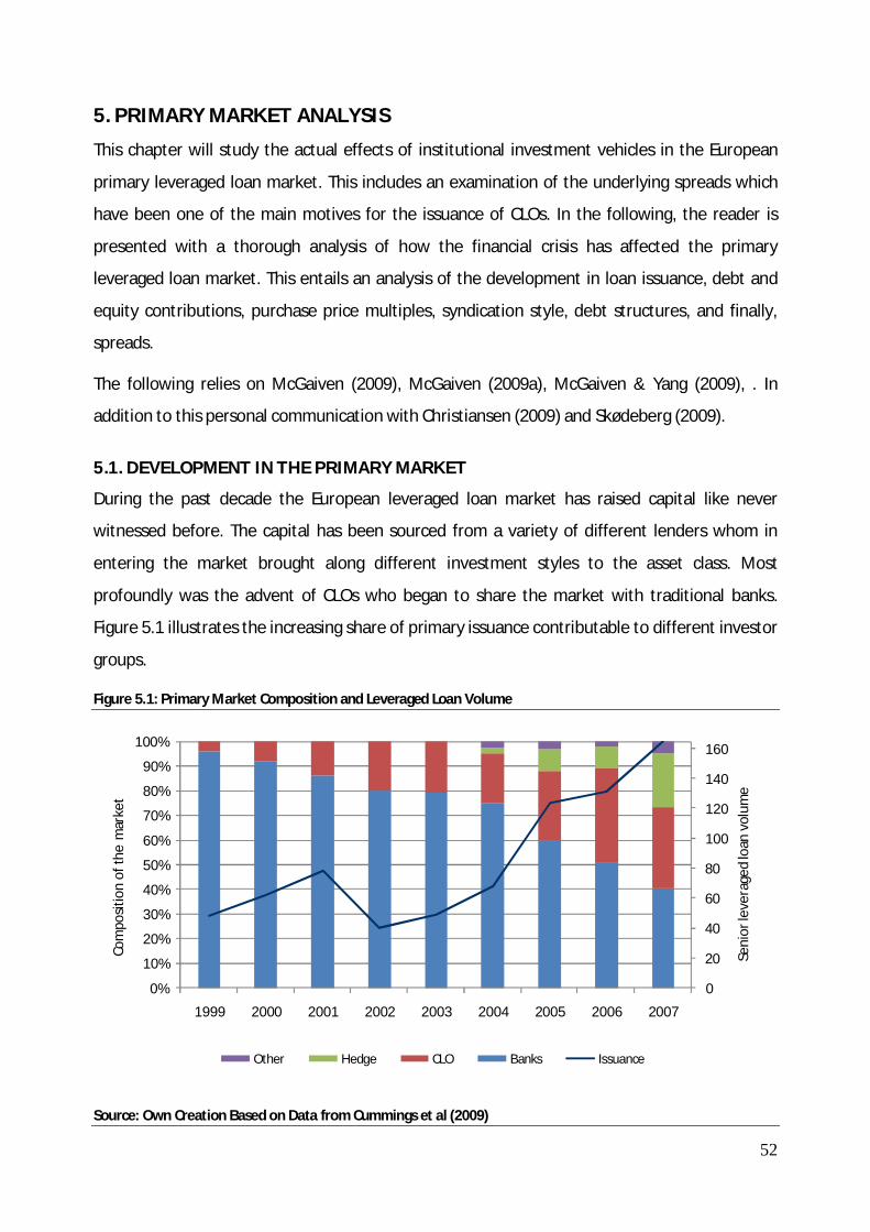
52

5. PRIMARY MARKET ANALYSIS

This chapter will study the actual effects of institutional investment vehicles in the European

primary leveraged loan market. This includes an examination of the underlying spreads which

have been one of the main motives for the issuance of CLOs. In the following, the reader is

presented with a thorough analysis of how the financial crisis has affected the primary

leveraged loan market. This entails an analysis of the development in loan issuance, debt and

equity contributions, purchase price multiples, syndication style, debt structures, and finally,

spreads.

The following relies on McGaiven (2009), McGaiven (2009a), McGaiven & Yang (2009), . In

addition to this personal communication with Christiansen (2009) and Skødeberg (2009).

5.1. DEVELOPMENT IN THE PRIMARY MARKET

During the past decade the European leveraged loan market has raised capital like never

witnessed before. The capital has been sourced from a variety of different lenders whom in

entering the market brought along different investment styles to the asset class. Most

profoundly was the advent of CLOs who began to share the market with traditional banks.

Figure 5.1 illustrates the increasing share of primary issuance contributable to different investor

groups.

Figure 5.1: Primary Market Composition and Leveraged Loan Volume

Source: Own Creation Based on Data from Cummings et al (2009)

0

20

40

60

80

100

120

140

160

0%

10%

20%

30%

40%

50%

60%

70%

80%

90%

100%

1999 2000 2001 2002 2003 2004 2005 2006 2007

Other Hedge CLO Banks Issuance

Seni

or le

vera

ged

loan

vol

ume

Com

posi

tion

of th

e m

arke

t

53

The European leveraged loan market was introduced to CLOs in 1999. Throughout the year

three institutional investment vehicles entered the market, all utilising cash flow CLOs to fund

investments in senior and mezzanine leveraged loans. The cash flow CLO applied a buy and hold

investment style which was similar to that utilised by banks. In their first year institutional

investors ended up accounting for 4.2% of the primary market.

During the following years, the total number of investors more than doubled compared to 1999

figures. Leveraged loan issuance in the year of 2001 was close to € 80 billion, of which

institutional investors had increased their share of the primary market to 13.9% - more than a

treble of the 1999 share. Cash flow CLOs remained the preferred investment vehicle,

maintaining the buy and hold investment style.

The year 2002 brought along the collapse of the telecom and cable industries, which in recent

years had influenced the debt markets tremendously. The following period, characterised by

increasing defaults, brought an end to the bull-run. Consequently, European leveraged loan

issuance was reduced by nearly 50 percent of the 2001 record high €78 billion issuance.

However, the overall commitment of the institutional investors proved consistent as their total

market share reached new levels of 20%.

The crisis occurring in 2002 would prove to be of little significance to the loan market whose

upturn was fast reverted. Throughout 2004, the increasing private equity activity drove volume

back to €67.8 billion of which funds contributed 25%. The leverage loan market attracted more

and more attention and new types of investment vehicles made their entry in the market. In

recognition of the increasingly growing institutional appetite, the way deals were structured

changed. This was reflected in the increasing availability of the more fund-friendly term loan

B/C.

2005 became the year in which the European leveraged loan market was truly revolutionised.

Leveraged loan issuance increased by nearly 100 percent to reach an astronomic €123.5 billion.

The ability of institutional investors to raise funding seemed without limitations as their total

market share hit 40%. The number of vehicles under their active management now accounted

for 126 provided by 53 different funds.

The evolution occurring during 2005 did not continue in 2006, which was characterised as a

year of consolidation. The market remained strong throughout the year, and while increases of

54

recent years were unobtainable, primary volume did rise to €131.3 billion. The involvement of

institutional investors, however, increased undauntedly and now accounted for 49.3% of the

primary market.

With institutional investors gradually appropriating the position as the majority player over

banks, 2007 appeared to be the year in which the European loan market would eventually carry

similar characteristics to that of the more developed U.S. market. For the 12 months ending

June 30, 2007, institutional investors accounted for 54.6% of new issuance while the

involvement of banks fell to an all-time low of 40.4%.

Furthermore, 2007 became the year in which CLOs finally lost their momentum as institutional

investors began to diversify investment strategies. This was predominantly attributable to

hedge funds becoming more desirable due to their somewhat more aggressive approach in

which capital arbitrage opportunities are sought.

Most influential, however, was the appearance of the credit crunch which hit the entire

financial system during the summer of 2007, and sent the European loan market into an abrupt

stand still. Banks and loan funds resigned as easy financing vanished and leveraged unwound.

The leveraged lending business experienced a fundamental change as recent years’ heavy

demand for leveraged loans all of a sudden disappeared.

CLOs were first in line to experience the new reality. With the onset of the credit crunch

institutional investors no longer desired structured finance products, making it extremely

difficult to raise new funds. With a share of leveraged loans funded by CLOs at 40% LTM, ending

June 2007, this obviously led to a massive hole in the investor base.

In addition, all funds structured to utilise mark-to-market approaches struggled significantly.

Just as market value CLOs had begun to gain momentum, they were severely influenced by the

steep decline in secondary market prices. This resulted in market value CLO managers

exclusively focusing on their existing portfolio in an attempt to avert a looming liquidation. This

left no spare attention to new fund issues.

5.1.1. The CLO Issuance Comes to an End

As earlier mentioned the cash flow CLO is an investment vehicle structured to generate

arbitrage. Basically, this arbitrage is achieved by taking advantage of the difference between

the payments associated with the collateral pool and the corresponding liabilities. In order to

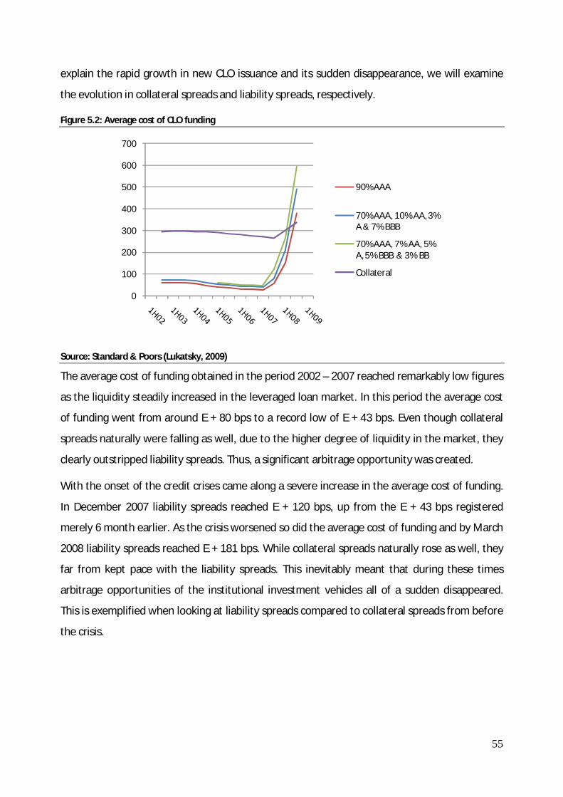
55

explain the rapid growth in new CLO issuance and its sudden disappearance, we will examine

the evolution in collateral spreads and liability spreads, respectively.

Figure 5.2: Average cost of CLO funding

Source: Standard & Poors (Lukatsky, 2009)

The average cost of funding obtained in the period 2002 – 2007 reached remarkably low figures

as the liquidity steadily increased in the leveraged loan market. In this period the average cost

of funding went from around E + 80 bps to a record low of E + 43 bps. Even though collateral

spreads naturally were falling as well, due to the higher degree of liquidity in the market, they

clearly outstripped liability spreads. Thus, a significant arbitrage opportunity was created.

With the onset of the credit crises came along a severe increase in the average cost of funding.

In December 2007 liability spreads reached E + 120 bps, up from the E + 43 bps registered

merely 6 month earlier. As the crisis worsened so did the average cost of funding and by March

2008 liability spreads reached E + 181 bps. While collateral spreads naturally rose as well, they

far from kept pace with the liability spreads. This inevitably meant that during these times

arbitrage opportunities of the institutional investment vehicles all of a sudden disappeared.

This is exemplified when looking at liability spreads compared to collateral spreads from before

the crisis.

0

100

200

300

400

500

600

700

90% AAA

70% AAA, 10% AA, 3% A & 7% BBB

70% AAA, 7% AA, 5% A, 5% BBB & 3% BB

Collateral

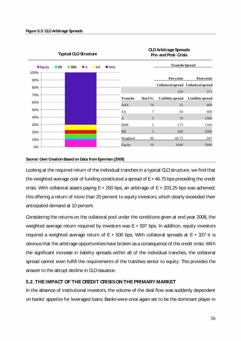
56

Figure 5.3: CLO Arbitrage Spreads

Source: Own Creation Based on Data from Eyerman (2009)

Looking at the required return of the individual tranches in a typical CLO structure, we find that

the weighted average cost of funding constituted a spread of E + 46.75 bps preceding the credit

crisis. With collateral assets paying E + 250 bps, an arbitrage of E + 203.25 bps was achieved;

this offering a return of more than 20 percent to equity investors, which clearly exceeded their

anticipated demand at 10 percent.

Considering the returns on the collateral pool under the conditions given at end year 2008, the

weighted average return required by investors was E + 597 bps. In addition, equity investors

required a weighted average return of E + 500 bps. With collateral spreads at E + 337 it is

obvious that the arbitrage opportunities have broken as a consequence of the credit crisis. With

the significant increase in liability spreads within all of the individual tranches, the collateral

spread cannot even fulfill the requirements of the tranches senior to equity. This provides the

answer to the abrupt decline in CLO issuance.

5.2. THE IMPACT OF THE CREDIT CRISIS ON THE PRIMARY MARKET

In the absence of institutional investors, the volume of the deal flow was suddenly dependent

on banks’ appetite for leveraged loans. Banks were once again set to be the dominant player in

Typical CLO StructureCLO Arbitrage Spreads

Pre- and Post- Crisis

0%

10%

20%

30%

40%

50%

60%

70%

80%

90%

100%

Equity BB BBB A AA AAA Tranche Spread

Pre-crisis Post-crisis

Collateral spread Collateral spread

250 373

Tranche Size (%) Liability spread Liability spread

AAA 70 25 400

AA 7 50 600

A 5 70 1000

BBB 5 175 1500

BB 3 450 5000

Weighted 90 46.75 597

Equity 10 1000 5000

57

the leveraged loan market, similar to the period preceding the blossoming private equity days -

although at this time at a far more limited level than earlier seen.

The leveraged finance departments, however, faced difficulties with existing credits which

limited their accessibility to the scarce capital internally at banks disposal. The credit

committees would immediately reject any commitments involving leveraged debt products,

even when presented with potentially attractive deals. Focus was now being directed towards

relationship borrowing and in particular investment-grade companies. Local corporate

businesses were preferred over weaker relationships of private equity sponsors across Europe.

In addition, the financial system went into total chaos as one of the world’s largest investment

banks, Lehman Brothers, filed for bankruptcy on September 15, 2008. The final pinch of

confidence in the banking system disappeared, and the interbank lending market collapsed -

leaving numerous banks nationalised, bailed-out, forcibly merged, or broken up.

In this new environment, characterised by large government intervention and decreasing

appetite for risk, banks in general made less capital available to be invested in leveraged

finance products - favouring more stable and high-quality assets.

The volume of new issuance in the leveraged loan market decreased significantly in the second

half of 2007 and for the whole of 2008, as a result of the shrunken investor base and

carefulness of the few lenders still possessing available cash.

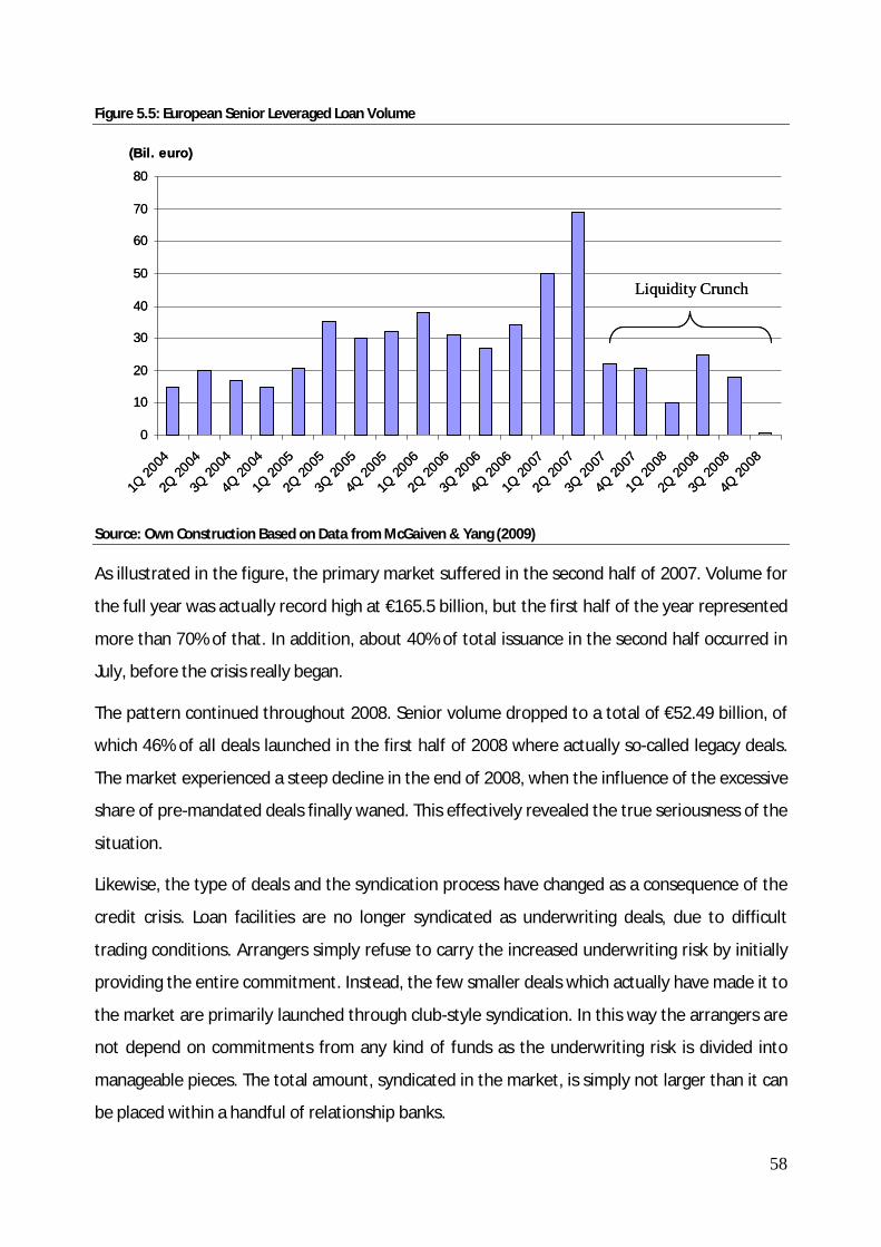
58

Figure 5.5: European Senior Leveraged Loan Volume

Source: Own Construction Based on Data from McGaiven & Yang (2009)

As illustrated in the figure, the primary market suffered in the second half of 2007. Volume for

the full year was actually record high at €165.5 billion, but the first half of the year represented

more than 70% of that. In addition, about 40% of total issuance in the second half occurred in

July, before the crisis really began.

The pattern continued throughout 2008. Senior volume dropped to a total of €52.49 billion, of

which 46% of all deals launched in the first half of 2008 where actually so-called legacy deals.

The market experienced a steep decline in the end of 2008, when the influence of the excessive

share of pre-mandated deals finally waned. This effectively revealed the true seriousness of the

situation.

Likewise, the type of deals and the syndication process have changed as a consequence of the

credit crisis. Loan facilities are no longer syndicated as underwriting deals, due to difficult

trading conditions. Arrangers simply refuse to carry the increased underwriting risk by initially

providing the entire commitment. Instead, the few smaller deals which actually have made it to

the market are primarily launched through club-style syndication. In this way the arrangers are

not depend on commitments from any kind of funds as the underwriting risk is divided into

manageable pieces. The total amount, syndicated in the market, is simply not larger than it can

be placed within a handful of relationship banks.

0

10

20

30

40

50

60

70

80

1Q 20

042Q

2004

3Q 20

044Q

2004

1Q 20

052Q

2005

3Q 20

054Q

2005

1Q 20

062Q

2006

3Q 20

064Q

2006

1Q 20

072Q

2007

3Q 20

074Q

2007

1Q 20

082Q

2008

3Q 20

084Q

2008

(Bil. euro)

Liquidity Crunch

0

10

20

30

40

50

60

70

80

1Q 20

042Q

2004

3Q 20

044Q

2004

1Q 20

052Q

2005

3Q 20

054Q

2005

1Q 20

062Q

2006

3Q 20

064Q

2006

1Q 20

072Q

2007

3Q 20

074Q

2007

1Q 20

082Q

2008

3Q 20

084Q

2008

(Bil. euro)

Liquidity Crunch

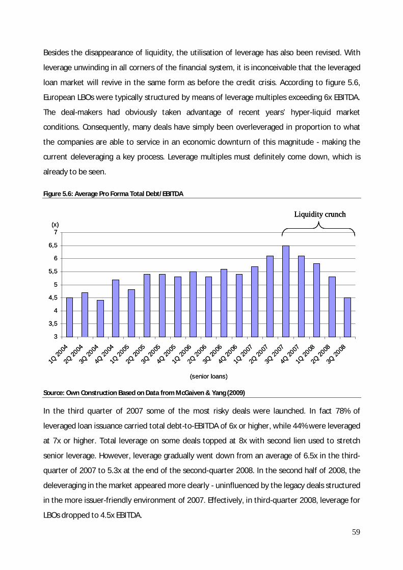
59

Besides the disappearance of liquidity, the utilisation of leverage has also been revised. With

leverage unwinding in all corners of the financial system, it is inconceivable that the leveraged

loan market will revive in the same form as before the credit crisis. According to figure 5.6,

European LBOs were typically structured by means of leverage multiples exceeding 6x EBITDA.

The deal-makers had obviously taken advantage of recent years’ hyper-liquid market

conditions. Consequently, many deals have simply been overleveraged in proportion to what

the companies are able to service in an economic downturn of this magnitude - making the

current deleveraging a key process. Leverage multiples must definitely come down, which is

already to be seen.

Figure 5.6: Average Pro Forma Total Debt/EBITDA


In the third quarter of 2007 some of the most risky deals were launched. In fact 78% of

leveraged loan issuance carried total debt-to-EBITDA of 6x or higher, while 44% were leveraged

at 7x or higher. Total leverage on some deals topped at 8x with second lien used to stretch

senior leverage. However, leverage gradually went down from an average of 6.5x in the third-

quarter of 2007 to 5.3x at the end of the second-quarter 2008. In the second half of 2008, the

deleveraging in the market appeared more clearly - uninfluenced by the legacy deals structured

in the more issuer-friendly environment of 2007. Effectively, in third-quarter 2008, leverage for

LBOs dropped to 4.5x EBITDA.

3

3,5

4

4,5

5

5,5

6

6,5

7

1Q 20

042Q

2004

3Q 20

044Q

2004

1Q 20

052Q

2005

3Q 20

054Q

2005

1Q 20

062Q

2006

3Q 20

064Q

2006

1Q 20

072Q

2007

3Q 20

074Q

2007

1Q 20

082Q

2008

3Q 20

08

(senior loans)

(x)Liquidity crunch

3

3,5

4

4,5

5

5,5

6

6,5

7

1Q 20

042Q

2004

3Q 20

044Q

2004

1Q 20

052Q

2005

3Q 20

054Q

2005

1Q 20

062Q

2006

3Q 20

064Q

2006

1Q 20

072Q

2007

3Q 20

074Q

2007

1Q 20

082Q

2008

3Q 20

08

(senior loans)

(x)Liquidity crunchLiquidity crunch

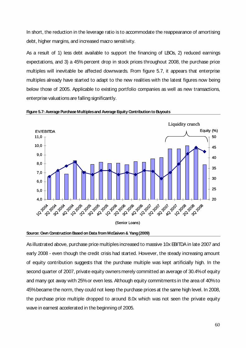
60

In short, the reduction in the leverage ratio is to accommodate the reappearance of amortising

debt, higher margins, and increased macro sensitivity.

As a result of 1) less debt available to support the financing of LBOs, 2) reduced earnings

expectations, and 3) a 45% percent drop in stock prices throughout 2008, the purchase price

multiples will inevitable be affected downwards. From figure 5.7, it appears that enterprise

multiples already have started to adapt to the new realities with the latest figures now being

below those of 2005. Applicable to existing portfolio companies as well as new transactions,

enterprise valuations are falling significantly.

Figure 5.7: Average Purchase Multiples and Average Equity Contribution to Buyouts


As illustrated above, purchase price multiples increased to massive 10x EBITDA in late 2007 and

early 2008 - even though the credit crisis had started. However, the steady increasing amount

of equity contribution suggests that the purchase multiple was kept artificially high. In the

second quarter of 2007, private equity owners merely committed an average of 30.4% of equity

and many got away with 25% or even less. Although equity commitments in the area of 40% to

45% became the norm, they could not keep the purchase prices at the same high level. In 2008,

the purchase price multiple dropped to around 8.0x which was not seen the private equity

wave in earnest accelerated in the beginning of 2005.

Liquidity crunch

4,0

5,0

6,0

7,0

8,0

9,0

10,0

11,0

1Q 20

042Q

2004

3Q 20

044Q

2004

1Q 20

052Q

2005

3Q 20

054Q

2005

1Q 20

062Q

2006

3Q 20

064Q

2006

1Q 20

072Q

2007

3Q 20

074Q

2007

1Q 20

082Q

2008

3Q 20

08

(Senior Loans)

EV/EBITDA

20

25

30

35

40

45

50Equity (%)

Liquidity crunch

4,0

5,0

6,0

7,0

8,0

9,0

10,0

11,0

1Q 20

042Q

2004

3Q 20

044Q

2004

1Q 20

052Q

2005

3Q 20

054Q

2005

1Q 20

062Q

2006

3Q 20

064Q

2006

1Q 20

072Q

2007

3Q 20

074Q

2007

1Q 20

082Q

2008

3Q 20

08

(Senior Loans)

EV/EBITDA

20

25

30

35

40

45

50Equity (%)

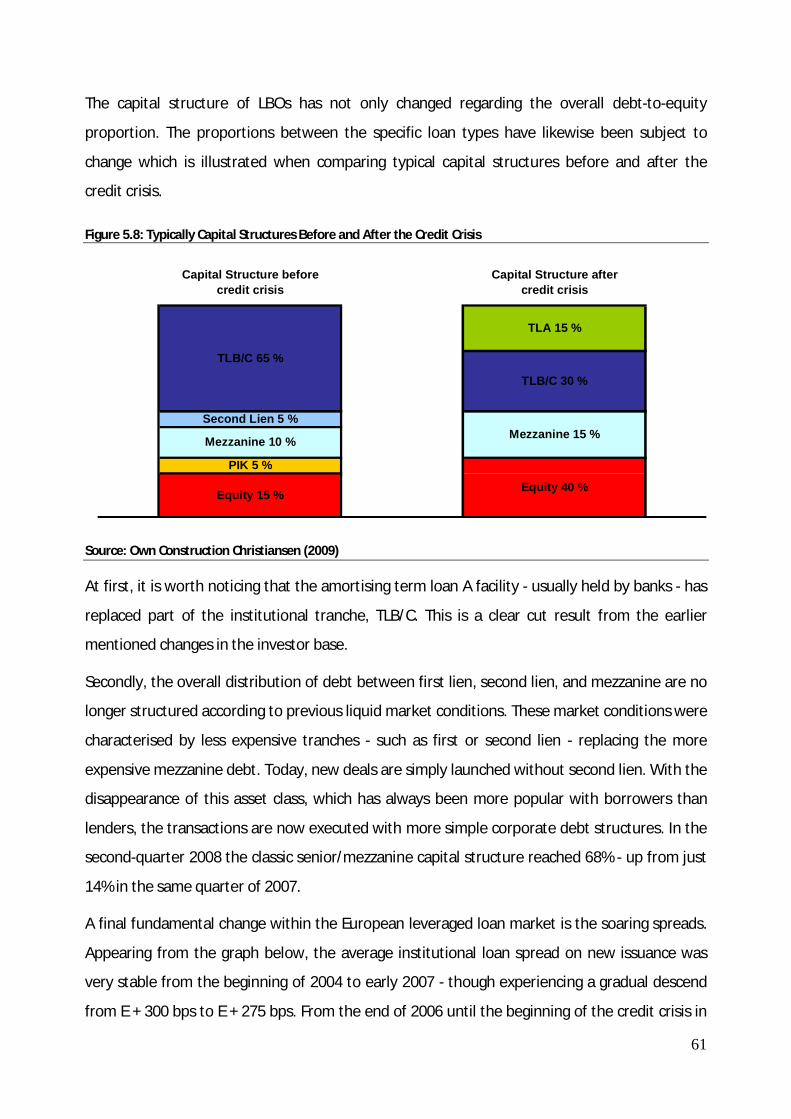
61

The capital structure of LBOs has not only changed regarding the overall debt-to-equity

proportion. The proportions between the specific loan types have likewise been subject to

change which is illustrated when comparing typical capital structures before and after the

credit crisis.

Figure 5.8: Typically Capital Structures Before and After the Credit Crisis

Source: Own Construction Christiansen (2009)

At first, it is worth noticing that the amortising term loan A facility - usually held by banks - has

replaced part of the institutional tranche, TLB/C. This is a clear cut result from the earlier

mentioned changes in the investor base.

Secondly, the overall distribution of debt between first lien, second lien, and mezzanine are no

longer structured according to previous liquid market conditions. These market conditions were

characterised by less expensive tranches - such as first or second lien - replacing the more

expensive mezzanine debt. Today, new deals are simply launched without second lien. With the

disappearance of this asset class, which has always been more popular with borrowers than

lenders, the transactions are now executed with more simple corporate debt structures. In the

second-quarter 2008 the classic senior/mezzanine capital structure reached 68% - up from just

14% in the same quarter of 2007.

A final fundamental change within the European leveraged loan market is the soaring spreads.

Appearing from the graph below, the average institutional loan spread on new issuance was

very stable from the beginning of 2004 to early 2007 - though experiencing a gradual descend

from E + 300 bps to E + 275 bps. From the end of 2006 until the beginning of the credit crisis in

Equity 40 %

TLB/C 30 %

Mezzanine 15 %

TLA 15 %

Capital Structure after credit crisis

TLB/C 65 %

Mezzanine 10 %

Capital Structure before credit crisis

Equity 15 %

PIK 5 %

Second Lien 5 %

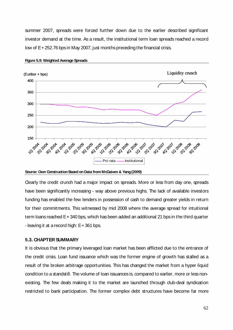
62

summer 2007, spreads were forced further down due to the earlier described significant

investor demand at the time. As a result, the institutional term loan spreads reached a record

low of E + 252.76 bps in May 2007, just months preceding the financial crisis.

Figure 5.9: Weighted Average Spreads


Clearly the credit crunch had a major impact on spreads. More or less from day one, spreads

have been significantly increasing - way above previous highs. The lack of available investors

funding has enabled the few lenders in possession of cash to demand greater yields in return

for their commitments. This witnessed by mid 2008 where the average spread for intuitional

term loans reached E + 340 bps, which has been added an additional 21 bps in the third quarter

- leaving it at a record high: E + 361 bps.


It is obvious that the primary leveraged loan market has been afflicted due to the entrance of

the credit crisis. Loan fund issuance which was the former engine of growth has stalled as a

result of the broken arbitrage opportunities. This has changed the market from a hyper liquid

condition to a standstill. The volume of loan issuances is, compared to earlier, more or less non-

existing. The few deals making it to the market are launched through club-deal syndication

restricted to bank participation. The former complex debt structures have become far more

150

200

250

300

350

400

1Q 20

042Q

2004

3Q 20

044Q

2004

1Q 20

052Q

2005

3Q 20

054Q

2005

1Q 20

062Q

2006

3Q 20

064Q

2006

1Q 20

072Q

2007

3Q 20

074Q

2007

1Q 20

082Q

2008

3Q 20

08

(Euribor + bps)

Pro rata Institutional

Liquidity crunch

150

200

250

300

350

400

1Q 20

042Q

2004

3Q 20

044Q

2004

1Q 20

052Q

2005

3Q 20

054Q

2005

1Q 20

062Q

2006

3Q 20

064Q

2006

1Q 20

072Q

2007

3Q 20

074Q

2007

1Q 20

082Q

2008

3Q 20

08

(Euribor + bps)

Pro rata Institutional

Liquidity crunch

63

simple and safe. The transactions have experienced a deleveraging process which has forced

the purchase price multiples down while the equity contribution has gone up. At the same

time, spreads have been rising due to the scarcity of investors. In this way it is clear that the

quality and yields of the few new deals making it to the market have improved significantly

from a lender perspective. It is, however, difficult to predict whether the improvements are

sufficient enough to bring back the investors.

First of all, the crux seems to be stability and investor confidence. The collapse of the secondary

market seems to be without an end – continuing to inhibit the primary market. Until arrangers

are somewhat certain that the bottom has been reached, they will remain on the sideline. With

the present market volatility, no arrangers are willing to take any underwriting risks on larger

deals. Evidently, one should not expect larger transactions to be executed any time soon.

Secondly, the debt structures might experience an evolution towards even more simplicity than

seen in today’s Senior/Mezzanine composition. Although there appears to be a decent appetite

among mezzanine funds, their required returns are getting closer to the equity sponsor’s own

expected returns. As a result, an all-senior deal seems more sensible. Rather than giving away

large non-call provisions, the sponsor may as well just put in a load of equity and keep the

option to refinance.

Finally, terms of the secondary market indicates that spreads need to go up and leverage

further down. Characterised as a quality note in the secondary market, TDC trades in the upper

80s by the end of 2008. The corresponding margins are at E + 200-250 bps while the

debt/EBITDA ratio equals 3.7x. Assuming a four-year maturity, these loans effectively yield E +

500-550 bps. Relative to actual primary market figures Q308, new deals are on average offered

with a debt/EBITDA of 4.5x and spreads at E + 360 bps. This strongly suggests that primary

issuance still has some catching up to do. For deals with leverage somewhere in the 3-4x

territory, spreads at E + 500-600 bps could be considered the target yield for new issuance.

The above mentioned predictions do not exactly prompt an optimistic view of new leveraged

lending activity in the near future. Even with improved terms and structures on new deals the

way ahead still allows for more improvements before leveraged loan issuances once again

become interesting investment objectives.

64

6. SECONDARY MARKET ANALYSIS

The forthcoming chapter contains an examination of the secondary leveraged loan market. This

entails a preliminary description of the development in the secondary trading activity – in which

the significantly improved market standards, and the increased number of institutional

investors, have played a key role. Subsequently, the chapter provides a thorough analysis of

how the financial crisis has made its mark on the loan prices in the secondary market. On the

basis of the current market conditions, we end the section with a view into 2009, to point out

the most looming risk factors in a new possible wave of forced selling.

The following relies on Bear (2007), McGaiven (2009), Taylor & Sansone (2006), Yang, Gupte &

Lukatsky (2009), King et al. (2009). In addition to this personal communication with Christiansen

(2009) and Skødeberg (2009).

6.1. DEVELOPMENTS IN THE SECONDARY MARKET

Making the leveraged loan market more efficient has been one of the most important recent

developments in the leveraged loan market. To compare the market to some of the more

traditional capital markets - such as bond and equity - the existence of greater transparency

and liquidity was required. The growth of institutional investor participation has brought along

major improvements in fulfilling these requirements.

First of all, the increased investor base has been the most influential factor for the foundation

of a true secondary market. The European loan market was exclusively dominated by banks

until the beginning of the century. Since these banks generally invested in loans with the

intention of holding them until maturity, there was little need for a secondary market.

However, the need for a reliable and liquid secondary market became evident as more

institutional investors entered the loan market through CLOs and hedge funds. With their focus

on an active total return management and trading, these investors are simply dependent on an

efficient secondary market in which they can actively manage their portfolios.

According to Taylor & Sansone (2006) the development of the secondary market is actually a

virtuous circle: “The development of a sophisticated nonbank lender base facilitates (and

increasingly is contingent upon) the development of a liquid secondary loan market”.

65

Starting in 1999, an increasingly liquid secondary market emerged as more institutional

investors entered the loan market. With their entrance more loans were traded - increasing the

liquidity of the secondary loan market. This encouraged more institutional investors to enter

the loan market - creating a self-reinforcing mechanism.

With the growth rate of primary loan issuance dependent on the secondary market becoming

more liquid - in order to fulfil institutional investor demands - several institutions and

individuals worked diligently to accelerate the liquidity process. Indeed, the organisation of the

Loan Syndication and Trading Association (LSTA) has been critical in developing trading norms

and settlement time frames.

One of the greatest differences between loan trades and stock or bond trades is how they

settle. Loans close on the exchange of negotiated documents because of their complexity,

whereas bonds and stocks settle electronically. Consequently, a previous lack of standardised

trade practices and documentation for purchasing, selling, or closing loans were a huge

obstacle. Closing a trade could easily take weeks.

Although the LSTA is not a regulatory authority, their intensive work within shortening and

facilitating this settlement process, has contributed significantly to the rapid development of a

more liquid secondary loan market. However, participants are still faced with difficulties in

closing their loan trades on a timely basis and in an efficient manner due to the nature of the

complicated settlement procedure.

The availability of pricing information is another important aspect that has enhanced the

transparency in the secondary loan market. In order to fulfil their more active investment

strategies, institutional investors need a reliable and independent source of prices on a regular

basis. As a result several banks, in particular investment banks, have established secondary

trading desks in the loan market, offering trade prices.

Although minimum assignments and transaction fees tend to impede liquidity to some degree,

trading costs are anticipated to decline concurrently with the market continuing to move

towards more standardised trading practises and documentation.

To sum up, it is obvious that the days of the secondary market as a sleepy backwater market in

terms of trade volume and liquidity is over. The secondary loan trading has improved

significantly as a result of several factors. First of all, the increased number of institutional

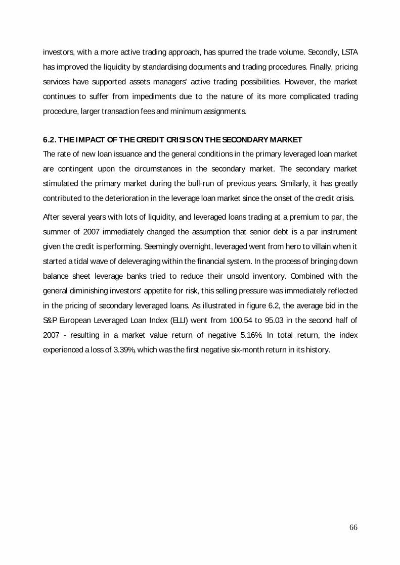
66

investors, with a more active trading approach, has spurred the trade volume. Secondly, LSTA

has improved the liquidity by standardising documents and trading procedures. Finally, pricing

services have supported assets managers' active trading possibilities. However, the market

continues to suffer from impediments due to the nature of its more complicated trading

procedure, larger transaction fees and minimum assignments.

6.2. THE IMPACT OF THE CREDIT CRISIS ON THE SECONDARY MARKET

The rate of new loan issuance and the general conditions in the primary leveraged loan market

are contingent upon the circumstances in the secondary market. The secondary market

stimulated the primary market during the bull-run of previous years. Similarly, it has greatly

contributed to the deterioration in the leverage loan market since the onset of the credit crisis.

After several years with lots of liquidity, and leveraged loans trading at a premium to par, the

summer of 2007 immediately changed the assumption that senior debt is a par instrument

given the credit is performing. Seemingly overnight, leveraged went from hero to villain when it

started a tidal wave of deleveraging within the financial system. In the process of bringing down

balance sheet leverage banks tried to reduce their unsold inventory. Combined with the

general diminishing investors' appetite for risk, this selling pressure was immediately reflected

in the pricing of secondary leveraged loans. As illustrated in figure 6.2, the average bid in the

S&P European Leveraged Loan Index (ELLI) went from 100.54 to 95.03 in the second half of

2007 - resulting in a market value return of negative 5.16%. In total return, the index

experienced a loss of 3.39%, which was the first negative six-month return in its history.

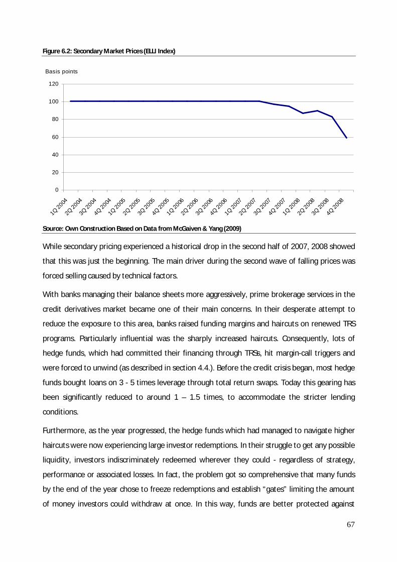
67

Figure 6.2: Secondary Market Prices (ELLI Index)


While secondary pricing experienced a historical drop in the second half of 2007, 2008 showed

that this was just the beginning. The main driver during the second wave of falling prices was

forced selling caused by technical factors.

With banks managing their balance sheets more aggressively, prime brokerage services in the

credit derivatives market became one of their main concerns. In their desperate attempt to

reduce the exposure to this area, banks raised funding margins and haircuts on renewed TRS

programs. Particularly influential was the sharply increased haircuts. Consequently, lots of

hedge funds, which had committed their financing through TRSs, hit margin-call triggers and

were forced to unwind (as described in section 4.4.). Before the credit crisis began, most hedge

funds bought loans on 3 - 5 times leverage through total return swaps. Today this gearing has

been significantly reduced to around 1 – 1.5 times, to accommodate the stricter lending

conditions.

Furthermore, as the year progressed, the hedge funds which had managed to navigate higher

haircuts were now experiencing large investor redemptions. In their struggle to get any possible

liquidity, investors indiscriminately redeemed wherever they could - regardless of strategy,

performance or associated losses. In fact, the problem got so comprehensive that many funds

by the end of the year chose to freeze redemptions and establish “gates” limiting the amount

of money investors could withdraw at once. In this way, funds are better protected against

0

20

40

60

80

100

120

1Q 20

042Q

2004

3Q 20

044Q

2004

1Q 20

052Q

2005

3Q 20

054Q

2005

1Q 20

062Q

2006

3Q 20

064Q

2006

1Q 20

072Q

2007

3Q 20

074Q

2007

1Q 20

082Q

2008

3Q 20

084Q

2008

Basis points

68

short-term run on their assets, which helps to avoid selling at fire-sale prices and, thus,

potentially relieve short-term market pressure. However, the trend is also causing tension

between investors, who may be in urgent need of cash, and managers, who may be more

interested in holding on to assets to protect their businesses. It appears to be a delicate matter

for managers to protect their own interests while acting to preserve the value of the portfolio

for investors.

Hedge funds have been forced to sell out en masse as a result of the above-mentioned

deleveraging process. The twin forces of executed investor redemptions and swaps hitting price

triggers has effectively left the loan prices in freefall.

In addition, several market value CLOs have breached their covenants due to severe losses in

their portfolio. When the value of the underlying collateral comes below a certain price level,

the CLO hit its market-value-trigger which forces the fund to unwind (as described in section

4.3.).

Managers looking to resolve market value issues are essentially faced with two options when

trying to avoid liquidation. They can either restructure the market value vehicle into a cash flow

CLO, or they can raise additional equity through asset sales or via equity injections. In a period

with shortage of capital, most subordinated investors found themselves in a position where

they chose not to “throw good money after bad”. Instead most market value CLOs have

deleveraged through a restructuring process where the best parts of the fund have created the

foundation for a new cash flow CLO.

For the hedge funds and market value CLOs, which did not mange to survive the above

mentioned difficulties, a total liquidation of the fund took place. Several funds tried to sell off

their loans in larger chunks through so-called Bids Wanted In Competition (BWIC), due to the

illiquid market conditions. This entails different dealers being allowed to make bids on the given

portfolio. With total BWIC activity rolled out in 2008, more than 40% higher over 2007, this

obviously created a tremendous selling pressure.

The outcome of the fund world pushing assets into a market already in its knees is depicted in

figure 6.2 above. In a vicious cycle of forced selling and falling prices, the average bid fell nearly

eight points from 95.03 to 87.07 in the first quarter 2008. With a total return of minus 8.56%

the performance was more than twice as bad as the previous part of the credit crisis.

69

In the second quarter of 2008, months of bleak outlooks were suddenly replaced with a

godsend gain in the market value. Given the horrors the market had suffered in January and

February, market participants obviously were reluctant to tempt fate in believing the market

would not crash again if more bad news appeared. However, it became clear that along with

the quarterly positive total return of around 5%, some market participants actually started to

gain faith in the market again. Earlier month’s downswing could be explained with technical

and liquidity driven factors rather than fundamental factors. Corporate balance sheets

generally seemed in good shape (at least outside the financial sector) and default rates of

senior secured loans were close to zero. It all appeared to be one of these great buying

opportunities which you would not miss in the world. As a result, buyers were spotted in the

market for the first time since the onset of the credit crisis - looking for what seemed to be

good corporate credits at heavily discounted prices.

However, just as modest optimism had returned into the market, the third and most severe

wave of falling prices accelerated. Up to this point, the collapse in secondary loan prices was

mainly due to technical factors, but in the second half of 2008 the threat of recession was

becoming ever more real. With a comprehensive economic slow-down at hand, outlooks of

inevitable rising default rates and signs of shockingly low recoveries, was the new reality. In a

risk adverse world, filled with distressed investors, the leveraged loan market turned into a true

nightmare of falling prices.

Starting above par during the summer of 2007, when the credit crisis began, the year ended

with prices around 95. In 2008, the prices just kept falling at a frightening pace. Investors’

portfolios lost a total of 30% over the course of the year. At first, the average prices in the ELLI

Index went below 80, then 70, and now the index has just moved below 60. The market players

are still waiting on the sideline to see how low they can go. Investors have learned from earlier

this year that it can be very costly to enter the market at what seems to be the bottom of this

total collapse in the secondary market prices.

6.2.1. Looking Into 2009

Fears of credit deterioration seem to be the most conspicuous risk factor in a new possible

wave of selling. Cash flow CLOs spent the first phase of the credit crunch largely protected by

par-value accounting, while in particular market value CLOs and hedge funds were exposed to a

70

tremendous pressure throughout 2008. However, as the loan performance switched from being

driven by technical factors to fundamental difficulties, it is now the turn of cash flow CLOs

managers to feel the “excitement”.

Signs of distressed credits sharpened significantly in the latter of 2008, as a result of the

declining corporate profitability. In mid-December 2008, LCD tracked 21 requests to amend or

waive financial covenants for the year - of which one-third was submitted in the fourth quarter

alone. In 2007, the total number of requests was merely five.

Furthermore, the share of issuers rated within the CCC/CC range in the ELLI Index more than

quintupled - from 0.22% to 1.25%. In addition, a report from S&P in December showed that the

share of CCC credit estimates had risen to 5.2% by mid- November 2008 - up from 3.4% at the

end-June 2008, and just 1.6% at the end of 2007.

Given these severe credit problems already witnessed in the end of 2008, CLO managers are

inevitably faced with a huge challenge consisting of a forthcoming wave of downgrades. While

most vehicles have certain maximum levels of CCC rated assets in their collateral portfolio, any

excess will have to be mark-to-market. As a consequence, it is a widespread market expectation

that a relatively large number of CLOs will experience difficulties in passing their over-

collateralisation tests.

As described in section 4.3, a breached OC test will trigger an event of default and all the cash

flows will be diverted to pay down interest and principal of the senior note holders in

compliance with the payment waterfall. At this juncture, the direct control of the CLO is

switched to the senior note holders, who can chose either to liquidate the CLO or follow the

payment waterfall and gradually delever over time. Although this would not automatically lead

to a massive round of forced selling, the controlling classes could opt to liquidate the portfolio

in a scenario where a large portion of CCC rated assets carry low market valuations.

In fact, a principal-agent conflict arises from the fact that CLO managers’ sub-advisor fees are

suspended due to the failed OC test. As figure 6.3 illustrates, in general more than 66% of

aggregate fees to CLO managers are effectively generated by the junior notes. Without these

fees CLO managers can become unable to maintain a minimum service platform, and may not

be able to meet operational service requirements or remain solvent. Especially in Europe, this

could become a problem since the CLO mangers usually do not have multiple funds creating a

71

stable fee platform. Given the insufficient payments accruing to the manager, one cannot

expect him to behave in the best interest of the investors - he simply has no incentive. This fact

could actually cause the CLO managers to trigger insolvency. Especially in cases when senior

note holders have chosen to reject requests concerning changes in the size of the CCC bucket.

Essentially, the senior note holder cuts off the main part of the managers’ payments which

leaves him no incentive to keep the CLO alive.

A round of liquidations could, however, be avoided through a consolidation among stand-alone

CLO platforms into larger asset managers. In this way more stable fee platforms are effectively

achieved and the vulnerability towards reduced management fees within the single CLO is

considerably mitigated.

Figure 6.3: Manager Reliance on Subordinated Fees

Source: Own Construction Based on Data from Eyerman et al (2009)


The secondary loan market has gone through a total meltdown since the onset of the credit

crisis in summer 2007. For the first time in history, the market has experienced a longer period

with negative returns. To begin with, in particular hedge funds and market value CLOs were

subject to a comprehensive deleveraging process. This lead to a vicious cycle of forced selling

and falling prices. The threat of a looming recession magnified as the crisis progressed, and

fundamental difficulties started to substitute technical factors. Bleak outlooks of rising default

0%

10%

20%

30%

40%

50%

60%

70%

80%

90%

100%

Equity BB BBB A AA AAA

Sub Fee

Senios Fee

0%

10%

20%

30%

40%

50%

60%

70%

80%

90%

100%

72

rates and low recovery rates pushed the market into a total hysteria of falling prices. At the end

of 2008, the average price of the ELLI Index stood at shockingly low 60 – these were loans that

for many years were traded at premiums to par. Looking into 2009, the cash flow CLO seems to

be the next investment vehicle experiencing difficulties. Given the severe economic slowdown,

there is a widespread expectation that some CLO mangers will breach their OC tests. Even

though this does not necessarily lead to a slew of forced selling, the CLO structure is once again

tested with respect to how well or badly it withstands the shocks of a downturn.

73

PART 4

Part 3 contained a thorough analysis of the primary and secondary leveraged loan market.

Initially, the reader was provided with an explanation of the rapid growth in both markets,

followed by an analysis of the effects from the credit crisis. It is clear that the increased

institutional investor base significantly stimulated the market conditions during the bull-run.

Likewise, they significantly contributed to the deterioration triggered by the credit crisis. The

leveraged loan market has suffered heavily from hedge funds and market value CLOs being

forced to unwind. This created a vicious self-reinforcing mechanism.

Effectively, part 3 has provided an analysis of the influences of institutional investors and the

credit crisis to the leveraged loan market.

Part 4 includes chapter 7 and 8. In this section the reader is presented with the theoretical

framework for pricing corporate debt when tranched according to priority. The model is

derived to enable the later comparison of the theoretically obtained debt value of ISS with

actual market prices. This allows for a determination of whether market prices are in

correspondence with theory. Careful considerations concerning estimation methods are made

to ensure the quality of the model output.

CLO structure






Part 2

Part 3

Chapter 2 & 3

Chapter 5 & 6

Chapter 7

Chapter 1

Chapter 9

Chapter 8

Chapter 4




Conclusion

Chapter 10

Chapter 11

Part 4

Part 5

74

7. THEORETICAL FRAMEWORK FOR PRICING CORPORATE DEBT

The following chapter provides for a derivation of the theoretical foundation for pricing

corporate debt when subordinated. On the basis of the Merton model (1974) and the Black

Scholes model (1973), a model for pricing corporate debt when sequentially tranched is initially

derived. Subsequently, the framework turns towards Leland (1994), who provides the

necessary theory for pricing corporate debt when treated as a coupon bond. Finally, the

theoretical framework of Leland is extended to handle debt when tranched in order of priority.

For a textbook treatment of section 7.1 see Lando (2004), and section 7.2 see Leland (1994). In

addition to this personal communication with Christiansen (2009) and Skødeberg (2009).

7.1 THE MERTON MODEL

The Merton model views a company’s equity as a call option on its assets in order to price the

shares of a company. Applying the put-call parity the value of a put can be priced analogously

to find the value of debt. The basic idea behind the model is to view all corporate securities

issued by a firm as contingent claims on the firm’s assets given the evolution of the market

value of these assets.

In the theoretical framework certain assumptions must be satisfied in order for the model to be

correct. The settings of the standard Black Scholes models are assumed satisfied, where

Agents are price takers, i.e. trading in assets has no effect on prices,

There are no transactions costs,

There is unlimited access to short selling and no indivisibilities of assets, and

Borrowing and lending through money-market account can be done at the same

riskless, continuously compounded rate 푟.

Given the time horizon is 푇, we wish to price a bond issued by a firm. Assuming that the value

of the firm’s assets follows a geometric Brownian motion, the stochastic process 푉 can be

expressed as

푑푉 = 휇푉 푑푡 + 휎푉 푑푊

75

where W is a standard Brownian motion, 휇 is the asset drift, and 휎 is the asset volatility. Both 휇

and 휎 are constants. Here dW represents the uncertainty in the price history of the assets.

Setting the initial value of the asset equal to V0, the equation yields the following solution

푉 = 푉 exp ((µ−σ2 ) 푡 + 휎푊 )

which is a log-normally distributed random variable.

Now assuming the existence of a money market account with a constant riskless rate 푟. The

price evolves deterministically as

훽 = exp (푟푡)

We know that the price 퐶 at time 0 of a contingent claim paying 퐶(푉 ) at time 푇 in an

economy consisting of these two assets equals

퐶 = 퐸 [푒푥푝 (−푟푡)퐶 ]

Expressing the value of 퐶 as the expected value of 퐶 discounted by the constant riskless rate

푟 at time 푡. Here 푄 is the equivalent martingale measure under which the dynamics of V are

given as

푉 = 푉 푒푥 푝 푟 −휎2 푡 + 휎푊

where 푊 is a Brownian motion. The replacement of 휇 with the constant riskless rate 푟 still

satisfies the requirement of a constant drift embedded in the Brownian motion.

It is worth remembering, that the present market value of the future cash flows generated from

an asset constitutes its market value. Any financing decisions made by the firm’s owners are

assumed without influence on the asset value.

To begin with our starting point is time 0 where we assume the firm has issued two types of

claims consisting of debt and equity. For simplicity we will in the initiating phase treat debt as a

zero-coupon bond with a face value 퐷 and a maturity date 푇 ≤ 푇. We are now able to express

payoffs to debt and equity at time 푇 as follows

Payoff to debt: 퐵 = min(퐷,푉 ) = 퐷 − max (퐷 − 푉 , 0)

Payoff to equity: 푆 = max (푉 − 퐷, 0)

76

by which the view of equity as a call option on the firm’s assets is exemplified. The underlying

reasoning is that equity owners run the firm. The equity owners will only exercise their call

option to pay off debt and retain ownership of the assets, when the total value of assets is

higher than the total value of the debt. In the reverse scenario, where the face value of debt

exceeds the value of the assets, equity owners are – due to limited liability – not obligated to

pay the face value of debt and realise a negative pay-off. Instead they will rather renounce

ownership and receive 0. Bond holders exercise their contingent claims and retain ownership of

the remaining assets. They thereby receive a recovery of 푉 which is less than the promised

face value of debt. Effectively, debt can be expressed as the difference between a riskless bond

and a put option.

With no corporate taxes or tax advantages associated with issuing debt, no other parties are to

receive any payments from 푉 which implies that the firm’s assets equal the value of debt and

equity

푉 = 퐵 + 푆

leaving the composition of the capital structure irrelevant as the relationship between debt and

equity is without influence to the value of the firm’s assets.

In order to value debt and equity prior to maturity date 푇, we incorporate Black Scholes

formula for pricing options to our perception of payoff to debt and equity. Thereby we obtain

the Merton model, as follows

Value of equity: 푆 = 퐶 (푉 ,퐷,휎, 푟,푇 − 푡)

Value of debt: 퐵 = 퐷푒푥푝 −푟(푇 − 푡) − 푃 (푉 ,퐷,휎, 푟,푇 − 푡)

where 퐶 and 푃 is the Black Scholes price of a European call and put option, respectively.

The face value of the bond, 퐷, constitutes the strike price while 푇 is time to maturity and 푟 is

the riskless rate. The unknown factors for later estimation then becomes the current level of 푉

at time 푡 and the corresponding volatility 휎 of the firm’s assets.

With the asset value equal to the value of debt and equity, debt can be expressed as

77

퐵 = 푉 − 퐶 .

The Merton model easily handles subordinated debt which is essential for the later valuation.

The model deals with subordination as depicted in table 7.1. The senior most secured debt has

a priority over junior debt, and can therefore be priced as if it were the only debt issue. Junior

debt can be priced according to its position in the subordination which is below senior and

above equity. When all senior debt has been repaid, the remaining value of the assets accrues

to junior bond holders to the point where the asset value equals their face value. Equity owners

will receive the value of the assets remaining after the senior and junior bond holders have

been repaid. This means that equity can be priced by viewing the entire debt as one class. Table

7.1 illustrates the payoffs to senior and junior debt and equity at maturity. The face values of

senior and junior debt represented are by 퐷 and 퐷 respectively.

Table 7.1: Payoff at maturity

Type of debt 푉 < 퐷 퐷 ≤ 푉 ≤ 퐷 + 퐷 퐷 + 퐷 < 푉

Senior 푉 퐷 퐷

Junior 0 푉 − 퐷 퐷

Equity 0 0 푉 − (퐷 + 퐷 ) Source: David Lando

With the payoff structure specified according to seniority an option representation can be

illustrated as in table 7.2. 퐶(푉,퐷) expresses the payoff at expiration of a call option. 푉 is the

value of the underlying asset while the face value of debt 퐷 represents the strike price.

Table 7.2: Option representation

Type of debt Option payoff

Senior 푉 − 퐶(푉,퐷 )

Junior 퐶(푉,퐷 ) − 퐶(푉,퐷 + 퐷 )

Equity 퐶(푉,퐷 + 퐷 ) Source: David Lando

The theoretical framework allows for a valuation of corporate debt when treated as a zero

coupon bond. Leveraged loans, however, are issued as coupon bonds which mean that the

78

theoretical approach must be extended to provide a solution to this issue. Leland (1994)

provides the necessary theory for pricing corporate debt incorporating continuous coupon

payment. Moreover, Leland’s model includes the tradeoff between the tax shield advantage of

issuing debt and the bankruptcy cost arising hereof.

7.2. THE LELAND MODEL

The Leland model follows that of Merton which means the earlier assumptions still apply.

However, some need alterations and additional assumptions must be satisfied, including

The activities of the firm are unchanged by financial structure,

Capital structure decisions, once made, are not subsequently changed,

The face value of debt, once issued, remains static through time,

A riskless asset that pays a constant rate of interest, 푟, exists.

The following theoretical framework allows for a valuation of time independent securities

which implies that the corporate debt issued is perpetual debt. Leveraged term loans are, in

general, issued with a maturity of approximately 7-10 years which justifies the assumption of

perpetual debt. The asset value of the firm still follows a geometric Brownian motion with

constant volatility and rate of return.

We now consider a claim on the firm that continuously pays a nonnegative coupon, 퐶, per

instant of time as long as the firm is solvent. The value of such a claim is denoted 퐹(푉, 푡). Since

the firm’s capital structure must remain constant after the initial issuance, the net cost of the

coupon can only be financed by issuing additional equity. From Black and Cox (1976) we know

that any such asset’s value must satisfy the partial differential equation

휎2 푉 퐹 (푉, 푡) + 푟푉퐹 (푉, 푡) − 푟퐹(푉, 푡) + 퐹 (푉, 푡) + 퐶 = 0

With the assumption of time independence satisfied, the term 퐹 (푉, 푡) = 0 and the equation

becomes an ordinary differential equation with 퐹(푉) satisfying

휎2 푉 퐹 (푉) + 푟푉퐹 (푉)− 푟퐹(푉) + 퐶 = 0

which general solution is

79

퐹(푉) = 퐴 + 퐴 푉 + 퐴 푉 , 푋 =2푟휎

where the constants 퐴 ,퐴 , and 퐴 are determined by boundary conditions.

With the general solution to the value of contingent claims presented, we turn to the specific

securities. The value of debt can be expressed 퐷(푉;퐶), where 퐶 is the constant perpetual

coupon payment promised unless the firm declares bankruptcy. For simplicity 퐶 is suppressed

as an argument and debt value is denoted 퐷(푉). The level of asset value at which bankruptcy is

declared is denoted 푉 . In the case of bankruptcy, a fraction 0 ≤ 훼 ≤ 1 of value will be lost to

bankruptcy costs. This leave debt holders with the value (1− 훼)푉 , and stock holders with

nothing. Boundary conditions are given as

푉 = 푉 ∶ 퐷(푉) = (1 − 훼)푉

푉 → ∞ ∶ 퐷(푉) →

When the asset value increases, bankruptcy becomes irrelevant and the value of debt will

approach the value of the capitalised coupon.

With the value of debt expressed in the general solution and the boundary conditions specified,

we are now able to determine the constants 퐴 ,퐴 , and 퐴 . With 푉 → ∞, we find that 푉 → 0

which implies 퐴 = 0 and 퐴 = . When 푉 = 푉 , we find 퐴 = (1− 훼)푉 − 푉 .

Consequently,

퐷(푉) =퐶푟 + (1− 훼)푉 −

퐶푟

푉푉

expresses the value of debt when issued as a coupon bond including bankruptcy costs.

The next step is to integrate the effects of taxes in the value of debt. The value of tax benefits

associated with debt financing resemble a security that pays a constant coupon equal to the

tax-sheltering value of interest payments, 휏퐶, as long as the firm is solvent and nothing in

bankruptcy. The value of the security is denoted 푇퐵(푉) and equals the value of tax benefits

associated with debt. Being time independent, it must satisfy the general solution with

boundary conditions

푉 = 푉 ∶ 푇퐵(푉) = 0

푉 → ∞ ∶ 푇퐵(푉) →

80

In the case of bankruptcy, the firm looses the tax benefits. Conversely, with increasing asset

value bankruptcy becomes irrelevant and the value of tax benefits approaches the capitalised

value of tax benefit. With the given boundary conditions, the general solution yields

푇퐵(푉) =휏퐶푟 −

휏퐶푟

푉푉

Tax legislation state, that deductibility of coupon payments is only achieved when these are

serviced by the firm’s earnings before interest and taxes. We assume that EBIT ≥ 퐶 is satisfied

at all times, and therefore the firm always benefits fully from the deductibility of coupon

payments when it is solvent. Thus, the equation above holds.

Debt issuance consequently implies tax deductibility of coupon payments which increases the

total value of the firm. Conversely, the possible bankruptcy costs related to debt issuance

reduce total firm value. The current value of a security 퐵퐶(푉), that pays no coupon, equals the

bankruptcy costs 훼푉 when 푉 = 푉 . This reflects the market value of a claim to 훼푉 if

bankruptcy is declared. The returns generated by this security are time independent, and

therefore, the security satisfies the general solution with boundary conditions

푉 = 푉 ∶ 퐵퐶(푉) = 훼푉

푉 → ∞ ∶ 퐵퐶(푉) → 0

We find that, as asset value increases, bankruptcy becomes irrelevant. Given these boundary

conditions the equation has the solution

퐵퐶(푉) = 훼푉푉푉

We are now able to express the total value of the firm as

푣(푉) = 푉 + 푇퐵(푉) − 퐵퐶(푉)

which in its full length appears as

푣(푉) = 푉 +휏퐶푟 1 −

푉푉 − 훼푉

푉푉

This allows for an expression of the value of equity which is the total value of the firm less the

value of debt.

퐸(푉) = 푣(푉)− 퐷(푉)

81

which in its full length appears as

퐸(푉) = 푉 − (1 − 휏)퐶푟 + (1− 휏)

퐶푟 − 푉

푉푉

We now need to decide whether 푉 is determined endogenously or exogenously. The former

implies that the issuing company is not restricted by covenants and therefore shareholders will

set the level of asset value at which bankruptcy is declared, 푉 , where the value of equity is

zero. The latter entails that debt is protected by positive net worth requirements restricted by

covenants. In the theoretical framework this entails that bankruptcy will be declared if the

asset value falls beneath the principal value of debt.

Leveraged loans are in general protected by covenants, working as a safeguard for investors to

position themselves against potential future defaults. To ensure debt holders that cash flows

generated by the issuing company are sufficient to service the debt, leveraged loan covenants

usually restrict a minimum value of EBITDA (see section 3.2.3.). It seems fair to assume that a

high correlation exists between asset value and EBITDA. On the basis of this, it is reasonable to

assume that leverage loan covenants restricting EBITDA can be translated to covenants

restricting the asset value. Effectively, we treat debt as protected by covenants restricting a

minimum level of asset value and consequently 푉 is determined exogenously.

When 푉 is exogenously determined, we assume that the principal value of debt corresponds

with the market value of debt when issued. This implies that 푉 = 퐷 . In relation to this, it must

be noted that minimum level of asset value should fulfill the requirements of share holders in

which the value of equity is equal to or greater than zero. From the equation expressing the

value of debt with 푉 = 퐷 , we are able to write the value of protected debt at issuance as a

function of the asset value, 푉 . The equation appears as

퐷 (푉 ) =퐶푟 + (1−∝)퐷 (푉 ) −

퐶푟

푉퐷 (푉 )

It is important to note that this equation only returns the value of debt at the initial asset value.

The equation expressing the value of debt with 푉 = 퐷 (푉 ) returns the value of debt as a

function of the asset value, 푉.

82

7.3. EXTENSION OF THE MODEL FRAMEWORK TO INCORPORATE SUBORDINATION

The theoretical approach provided by Leland prices the total debt of the company without

regards for a differentiation of debt. Leveraged buyouts are, however, typically structured with

several tranches ranked according to priority. We therefore need to modify the model to

handle subordination.

We look at total debt issuance as consisting of the different parts of debt - ranging from the

senior most secured to the most junior unsecured. Total coupon must equal

퐶 = 퐶 + 퐶 + 퐶

where 퐶 , 퐶 , and 퐶 represents the coupon to senior, second lien, and junior

debt, respectively. In this definition only three types of debt issues are included. However, the

specific composition of debt instruments varies greatly from company to company.

Total value of debt must equal

퐷(푉;퐶) = 퐷(푉;퐶 ) + 퐷(푉;퐶 ) + 퐷(푉;퐶 )

where the different coupon payments are those observed within the specific tranches. The

essential difference between senior and junior debt is their respective priority claim in the case

of bankruptcy. We know that only a fraction of (1− 훼)푉 accrues to debt holders when

bankruptcy is declared. According to priority this fraction will solely accrue to senior debt

holders until the repayment of their entire principal is satisfied. Any remaining recovery will

accrue to the second lien debt holders until their entire principal is repaid. Finally, junior debt

holders will receive whatever remains. When 푉 = 푉 , the value of debt issues, ranked in order

of priority, can be expressed

퐷 (푉 ) = min ((1− 훼)푉 ;푉 , )

퐷 (푉 ) = min (1− 훼)푉 − 퐷 (푉 );푉 ,

퐷 (푉 ) = min (1− 훼)푉 − 퐷 (푉 ) + 퐷 (푉 ) ;푉 ,

where 푉 , of debt, 푖 = {푆푒푛푖표푟;푆푒푐표푛푑 퐿푖푒푛; 퐽푢푛푖표푟}, expresses the notional value of the

specific tranches. Furthermore, any given value of debt must satisfy 퐷 (푉 ) ≥ 0 as debt holders

will never experience an additional loss in the case of bankruptcy.

83

From the equation expressing the value of debt, we know that the value of the continuous

coupon until bankruptcy equals

퐶푟 1 −

푉푉

and the value of the repayment in case of bankruptcy equals

(1 − 훼)푉푉푉

where represent the value of receiving 1 when 푉 hits 푉 , given the value today is 푉.

The principal value of senior, second lien, and junior debt are

퐷 (푉 ;퐶 ) =퐶푟

1 −푉푉

+ min (1 − 훼)푉 ;푉푆,0푉푉

퐷 (푉 ;퐶 ) =퐶

푟1−

푉푉

+ min (1− 훼)푉 − 푉푆,0;푉2푛푑 푙푖푒푛,0푉푉

퐷 푉 ;퐶 =퐶푟

1−푉푉

+ min (1− 훼)푉 − 푉푆,0 + 푉2푛푑 푙푖푒푛,0 ;푉퐽,0푉푉

where any given 푉 , ∗ equals 퐷 (푉 ).

This entails two scenarios to which debt can be priced depending on the relationship between

푉 , and (1 − 훼)푉 . We begin with the scenario where 푉 , ≥ (1− 훼)푉 to which we have

already provided the solution to 퐷 (푉 ;퐶 ) as

퐷 (푉 ;퐶 ) =퐶푆푟 1−

푉푉퐵

−푋

+ (1− 훼)푉퐵푉푉퐵

−푋

Consequently, the value of debt junior to 퐷 푉 ;퐶 is

푋 =퐶푟 1 −

푉푉

as all recovery accrue to senior debt holders.

We now turn to the derivation of 퐷 (푉 ;퐶 ) when 푉 , ≤ (1− 훼)푉 and find

84

퐷 (푉 ;퐶 ) =퐶푆푟 1−

푉푉퐵

−푋

+ VS,0푉푉퐵

−푋

Which under the assumption that returned recovery can be placed in debt with similar

characteristics is

퐷 (푉 ;퐶 ) =

퐶푆푟 1− 푉

푉퐵

−푋

1− 푉푉퐵

−푋 =퐶푆푟

When full recovery is achieved in the case of bankruptcy, we find that the value of senior debt

equals the value of the continuously compounded coupon - implying that the senior tranche is

risk free. This is caused by the models deterministic approach to valuation of debt. Given the

constant fraction lost to bankruptcy costs and certainty of the exact asset value when

bankruptcy occurs, investors can pre-determine the exact amount of recovery returned when

bankruptcy is triggered. However, it seems to be an invalid assumption that bankruptcy costs

can be pre-determined given the uncertainties surrounding this variable. For example, it

appears impossible to determine whether the company can be sold as a going concern or has to

be liquidated in the case of bankruptcy - two scenarios which imply widely different bankruptcy

costs.

In addition, the model assumes that an amount equal to (1 − 훼)푉 will be returned to debt

holders when bankruptcy is triggered as 푉 = 푉 . For bankruptcy to be triggered at the exact

moment 푉 = 푉 would require that asset value is constantly monitored which is not the case.

Consequently, it is fair to assume that bankruptcy might be declared in situations where 푉 <

푉 . This entails the asset value at bankruptcy not necessarily equals 푉 , and therefore the total

amount accruing to the investor as recovery will be less than initially assumed4.

In an attempt to circumvent these deterministic drawbacks of the model - which is especially

reflected when pricing subordinated debt - we argue that the pricing of each individual tranche

should be based on the likelihood of various recoveries to be realised. This is achieved by

calculating the price of the individual debt tranche under different scenarios of ∝ ranging from

0-1 which implies that the debt will be priced where 푉 , ≥ (1−∝)푉퐵 and 푉 , ≤ (1−∝)푉퐵. The

4 Leland (2006) provides a solution in which a simple mixed jump-diffusion process for firm value is treated. This will however not be included in this paper.

85

price returned in each individual scenario is then weighted by the probability of the specific

recovery to be returned to investors.

We have chosen only to change the fraction lost to bankruptcy costs and let 푉 remain

constant. The reason is that changing both alpha and 푉 does not necessarily provide a more

accurate result, but merely returns more scenarios of the actual recovery returned in case of

bankruptcy. In this way, the changes applied to alpha are meant to represent the combination

of the two abovementioned uncertainties.

The individual debt tranches are still priced according to priority. However, the prices are

obtained under various scenarios corresponding with expected probability of the specific

recovery achieved. We have chosen to let the probability follow that of a binomial distribution

which easily handles the determination of whether recovery is achieved or not. By including

∝= 0 the scenario where debt is returned at maturity is represented.


On the basis of the theoretical approach for valuation of corporate debt provided by Leland

(1994), we have derived a model which handles subordination of debt when treated as a

coupon bond. This implies that the senior most secured debt will only be affected according to

its share size, while the most junior debt will be affected severely as it in addition to its own risk

carries the risk of all debt senior to it. In addition, the deterministic drawback of the model has

been limited by assuming various recoveries can be obtained when bankruptcy actually occurs.

This is achieved by calculating the price returned under different recoveries weighted by the

probability of the specific fraction lost to bankruptcy. With this approach the priority of the

individual debt tranches remains unaffected and no tranche will be priced as a risk free

investment.

86

8. THEORETICAL FRAMEWORK OF INPUT ESTIMATION

This chapter concerns approaches for estimation of the inputs needed in the model framework.

Following a brief introduction of the different valuation methods available, the relative

valuation approach is examined. In relation to this, the application of EBITDA will be discussed.

Subsequently, we turn to the estimation of volatility and in continuation hereof, whether to

measure volatility of the stock or of the enterprise value. Finally, the complicated matter of

determining the fraction lost to bankruptcy costs is examined.

The following relies on McClure (2006), Plenborg & Petersen (2005), Raahauge (2009), Smith

(2007), Zucchi (2006). In addition to this personal communication with Christiansen (2009) and

Skødeberg (2009).

8.1. ESTIMATING ENTERPRISE VALUE

Determining a fair value of a company is a complicated and time consuming process. Being able

to estimate the right inputs used in the chosen valuation model demands a comprehensive

analysis within strategy, accounting and finance. The range of different valuation

methodologies can be divided into four fundamental categories depending on their

approaches. Figure 8.1 illustrates these, as follows:

Figure 8.1: Valuation models

Source: Plenborg (2000)

Valuation models

Absolute valuation models Liquidation valuation models Real option modelsRelative valuation models

DCF P/E Short term

EVA-model P/book Long term

Earnings-capitalisation-model EV/sales

Dividend discount model

Residual income model

EV/EBIT

EV/EBITDA

Valuation models

Absolute valuation models Liquidation valuation models Real option modelsRelative valuation models

DCF P/E Short term

EVA-model P/book Long term

Earnings-capitalisation-model EV/sales

Dividend discount model

Residual income model

EV/EBIT

EV/EBITDA

87

Several studies show that the absolute and relative valuation methodologies are the most

widely used in practise. The usage of the different models within each of the two categories

varies according to the specific purpose and surroundings of the company.

The liquidation method is typically only used in connection with companies experiencing a

financial crisis while real options barely applies in situations characterised by great uncertainty

about the future development.

We have chosen to apply a relative valuation approach in the later ISS case, because EV/EBITDA

is a commonly accepted multiple indicating the cash flows ability to cover the purchase price of

leveraged buyouts. As a consequence, the following sub-sections contain a brief introduction to

general market multiple analysis and a theoretical exposition of our specific use of the

EV/EBITDA multiple.

8.1.1. Relative Valuation Approach

Relative valuation is often referred to as a “quick and dirty” way to determine the value of a

company. Consequently, the utilisation of comparative multiples is among the favourite

valuation methodologies in practise. The underlying concept is straightforward: The value of a

company is determined in relation to how comparable companies are priced in the market.

Among public traded peers the procedure is as follows:

Create a list of comparable companies5 (industry peers) and obtain their market

values.

Convert these market values into comparable trading multiples, such as P/E, price-

to-book, EV/EBIT or EV/EBITDA.

Utilise the multiples of the peers to calculate a fair value of the target company.

The general problem concerning comparative multiples is the misleading assumption of the

procedure as a convenient and simple approach. This is simply a theoretical mistake which

easily can lead to wrong conclusions. In order to compare trading multiples within peer-groups6

the following fundamental assumptions must be satisfied:

5 Alternatively, data from previous comparable transactions can be used. 6 Companies within the same industry

88

The companies must bear the same risks7

The same accounting principles must be applied

The expected growth rates must be equal

It is obvious that such “carbon copies” do not exist in any industry. Theoretically, this leads to a

necessary adjustment of the multiples, reflecting the different surroundings in which the

companies find themselves. In practise, this implies that there are typically substantial

differences in the companies’ valuation multiples within the same peer group. Whether a

company is traded at a discount or premium to its peers is normally determined by a mixture of

several factors within all of the above mentioned areas. Effectively, the challenge for investors

is to spot the fundamental differences between comparable companies that might affect the

multiples. This enables the investor to figure out whether a specific company deserves a higher

or lower multiple than its peers.

Enterprise multiples estimate the value of a company on a debt-free basis. In this way the

effect of financial gearing is avoided. EBIT is typically applied in the denominator which ensures

consistency as this effectively measures earnings, assuming the company to be debt-free. To

avoid possible differences in depreciation policies, EBITDA may be preferable (clarified in the

following section). Figure 8.2 illustrates how the multiples EV/EBIT and EV/EBITDA look at a

company as a potential acquirer would - taking debt into account. Financial ratios like P/E or

P/Bonly look at the equity side of a company. Consequently, the latter ratios are simply not

appropriate when a company’s enterprise value needs to be estimated.

7 This includes financial as well as operational risk

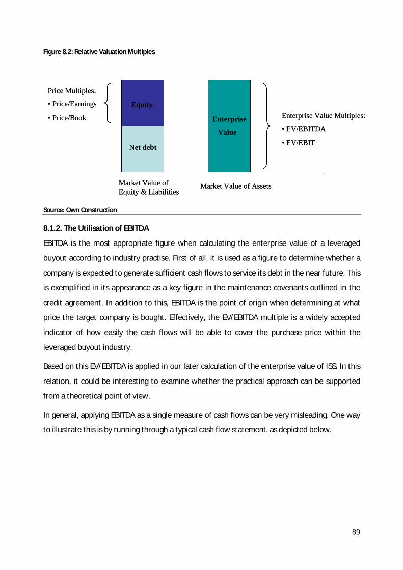
89

Figure 8.2: Relative Valuation Multiples


8.1.2. The Utilisation of EBITDA

EBITDA is the most appropriate figure when calculating the enterprise value of a leveraged

buyout according to industry practise. First of all, it is used as a figure to determine whether a

company is expected to generate sufficient cash flows to service its debt in the near future. This

is exemplified in its appearance as a key figure in the maintenance covenants outlined in the

credit agreement. In addition to this, EBITDA is the point of origin when determining at what

price the target company is bought. Effectively, the EV/EBITDA multiple is a widely accepted

indicator of how easily the cash flows will be able to cover the purchase price within the

leveraged buyout industry.

Based on this EV/EBITDA is applied in our later calculation of the enterprise value of ISS. In this

relation, it could be interesting to examine whether the practical approach can be supported

from a theoretical point of view.

In general, applying EBITDA as a single measure of cash flows can be very misleading. One way

to illustrate this is by running through a typical cash flow statement, as depicted below.

Enterprise Value Multiples:

• EV/EBITDA

• EV/EBIT

Enterprise

Value

Market Value of AssetsMarket Value of Equity & Liabilities

Net debt

Equity

Price Multiples:

• Price/Earnings

• Price/Book Enterprise Value Multiples:

• EV/EBITDA

• EV/EBIT

Enterprise

Value

Market Value of AssetsMarket Value of Equity & Liabilities

Net debt

Equity

Price Multiples:

• Price/Earnings

• Price/Book

90

Figure 8.3: Cash Flow Statement

Source: Plenborg (2002)

Starting with the operating profit (EBIT), we add the non-cash items - depreciation and

amortisation - to obtain EBITDA. At this point in the cash flow statement, we get to the

measure which is commonly used in the leveraged buyout industry as a shortcut to estimate

what is essential: The cash flows available to investors. However, in order to use EBITDA as a

true measure, reflecting the actual cash flow, it needs to be adjusted with respect to the main

differences between the two items. Working our way down the cash flow statement, it appears

that there are several factors which are not incorporated in EBITDA, but still affects the cash

flow. The most important ones are: (1) Net Working Capital (NWC) and (2) Capital Expenditures

(CAPEX).

Changes in working capital are the cash needed to cover day-to-day operations. Private equity

funds are known to pay great attention to the optimisation of operations due to their high

leverage. In their attempt to make the company as lean as possible, minimisation of net

working capital is an area of great importance. According to leveraged finance specialists, it is,

thus, widely accepted that NWC is left out when predicting the future cash flows.

Capital investments are typically sized according to the current conditions of the company. In

periods characterised by lower earnings a company will usually attempt to minimise its capital

investments, whereas higher earnings allows for increased capital expenditures. As a result,

CAPEX appears to disturb the transparency in the actual cash flows generated from the

Sales Revenue- Operating Costs

= Cash Flow from Operations

+/- Change in Working Capital (Current Assets and Current Liabilities)

= Operating Profit (EBIT)

- Taxes (from Operating Profit)

= Cash Earnings

+ Depreciation and Amortisation

+/- Net investments

= Free Cash Flow (Available to Lenders and Owners)

= EBITDA

91

underlying business. Thus, including CAPEX in determining the expected cash flows available to

service debt holders can provide a misleading result. From a lender perspective it is actually

more important to know what a company generates in cash flows before capital expenditures.

Effectively, the negligence of capital expenditures in EBITDA seems of little importance.

Although it can be argued that capital expenditures should not be included when determining

the expected cash flows available to service debt holders, they cannot completely be ignored.

Even though depreciation and amortisation are non-cash items added back to EBIT, they will

inevitably become relevant as equipment wears out. As a result, EBITDA should be subtracted

an amount reflecting the expenses needed to upgrade or replace worn out equipment to

achieve a more accurate measure of the actual cash flow.

In this relation, it would be obvious to set CAPEX equal to depreciation. However, this will often

not provide the true picture of the needed capital investments, as certain assets, like buildings

and cars, are depreciated according to accounting principles - generally not reflecting their true

wear. Instead it is more important to understand the underlying operations generating the cash

flows. In this way the needed capital investments to achieve a steady state can be found. This

level of capital expenditures is referred to as “maintenance CAPEX” and is highly dependent on

the investment needs within the specific industry. Thus, EBITDA should theoretically be

subtracted the maintenance CAPEX to achieve a more accurate measure of the cash flows

available to service the debt holders. However, estimating maintenance CAPEX is a subjective

assessment and it can be discussed if adjusting EBITDA for this amount gives a truer picture

than neglecting it.

When all is said and done, “cash is king” still applies, since cash flows show the true profitability

of a company. From this perspective, the utilisation of EBITDA as a single measure of the actual

cash flow can therefore be very misleading. However, regarding leveraged buyouts, the need

for cash is a crucial matter - making EBITDA a better proxy of the true cash flows relative to

other companies. Effectively, we argue that the practical utilisation of EBITDA, as a measure of

a company’s ability to service debt, can be supported from a theoretical point of view.

With the correspondence between the practical approach and the theoretical foundation, we

find that an application of the EV/EBITDA multiple will allow us to achieve an appropriate

estimate of the enterprise value of ISS.

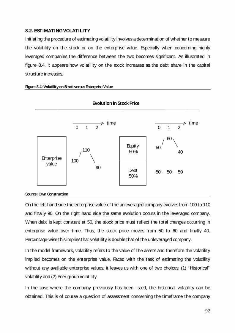
92

8.2. ESTIMATING VOLATILITY

Initiating the procedure of estimating volatility involves a determination of whether to measure

the volatility on the stock or on the enterprise value. Especially when concerning highly

leveraged companies the difference between the two becomes significant. As illustrated in

figure 8.4, it appears how volatility on the stock increases as the debt share in the capital

structure increases.

Figure 8.4: Volatility on Stock versus Enterprise Value


On the left hand side the enterprise value of the unleveraged company evolves from 100 to 110

and finally 90. On the right hand side the same evolution occurs in the leveraged company.

When debt is kept constant at 50, the stock price must reflect the total changes occurring in

enterprise value over time. Thus, the stock price moves from 50 to 60 and finally 40.

Percentage-wise this implies that volatility is double that of the unleveraged company.

In the model framework, volatility refers to the value of the assets and therefore the volatility

implied becomes on the enterprise value. Faced with the task of estimating the volatility

without any available enterprise values, it leaves us with one of two choices: (1) “Historical”

volatility and (2) Peer group volatility.

In the case where the company previously has been listed, the historical volatility can be

obtained. This is of course a question of assessment concerning the timeframe the company

Enterprise value

Equity 50%

Debt 50%

time time0 1 2 0 1 2

90

110

100

505050

40

60

50

Evolution in Stock Price

93

has been de-listed and the amount of available historical values obtainable. The second

approach is to estimate the volatility by measuring the historical volatility of a peer group of

listed competitors where enterprise values are available. The latter will be the approach utilised

in this paper, as this includes the impact on volatility resulting from the financial crisis.

To estimate volatility we have chosen to employ the Equally Weighted Moving Average

(EWMA) approach8. This is described by following equation

휎 =1푁 푟

To begin with we must obtain a time series of the underlying asset. The time period selected

should be limited when an estimation of the current volatility is desirable. However, the shorter

the period the higher are the chances of estimation errors. In short, this means a tradeoff

between precision and relevance. Since we initially are unable to tell which time span will

create the best result we employ the Root Mean Squared Error (RMSE) approach to measure

the fit. This is described in the equation below

푅푀푆퐸 =1푇 (푟 − 휎 )

푅푀푆퐸 measures the average distance between the realised and predicted volatility. The time

length resulting in the smallest 푅푀푆퐸 is preferable.

8.3. THE FRACTION 휶 LOST TO BANKRUPTCY COSTS

Determining the fraction lost to bankruptcy costs is a very complicated matter. The extensive

amount of empirical studies, which, in vain, have struggled to provide a fair estimate of the

costs associated with bankruptcy, indicates the degree of complexity surrounding the

approach. Consensus in the performed studies is, however, achieved concerning which factors

8 Since the focus of this paper is on pricing of leveraged loans and not volatility estimation, we will refrain from employing several models to find the best measure of volatility.

94

are the most influential. In general, bankruptcy costs can be divided into two categories: (1)

Direct costs and (2) Indirect costs.

The direct costs manly consist of tangible expenses such as fees to lawyers, accountants,

restructuring advisors, turnaround specialists, etc.. With these expenses relatively easy to

identify it seems reasonable to believe that a fair estimate can be achieved.

The indirect costs consist of an extensive range of unobservable opportunity costs. For

example, customers opting out on dealing with a firm entering bankruptcy might result in lost

sales and profits. The firm may as well face increased costs related to poorer terms with

suppliers due to the financially vulnerable position. Furthermore, lost opportunities resulting

from management’s diversion - running a distressed firm - is also included in the indirect costs.

From an investor perspective, predicting the unobservable effects, resulting from entering

financial distress and the subsequent bankruptcy, is more or less impossible. Therefore, the

best estimation will often rely on historical industry specific recovery rates along with empirical

studies of similar firms, assuming these studies display relatively high consistency.


In the process of determining the most appropriate valuation method for estimation of the

enterprise value, we find that market participants in general apply the EV/EBITDA multiple

approach. The underlying reasoning is that leveraged buyout practitioners primarily focus on

how well cash flows of the acquired company can cover the purchase price. In this relation,

EBITDA is generally assumed the best proxy for the actual cash flow.

With respect to its later application, volatility is to be found on the enterprise value utilising the

Equally Weighted Moving Average approach. In addition, the Root Mean Squared Error is

employed to ensure the most accurate estimation is chosen. Finally, we found that the task of

determining the fraction lost to bankruptcy costs is a process of great difficulty surrounded by

high uncertain. The best estimate will in this relation rely on historical recovery rates and

empirical studies.

95

PART 5

In part 4 Leland’s model framework was extended to handle subordination of debt. To

circumvent the deterministic drawbacks of the model, prices should be obtained under various

scenarios of alpha weighted by the possibility of their occurrence. The subsequent examination

of input estimations, revealed the most appropriate approaches. Effectively, we are now

capable of pricing leveraged loans from a theoretical point of view.

In this way, part 4 provides a derivation of a theoretical approach to pricing leveraged loans.

Part 5 includes chapter 9, 10 and 11. The section contains a case study of ISS in which the

institutional knowledge concerning the leveraged loan market and the derived model for

pricing leveraged loans are applied. Beginning with an estimation of the various inputs needed

in the model framework, the section moves on to an actual model implementation. This

provides us with the prices of ISS’s individual debt tranches. Subsequently, we compare the

prices returned by the model with actual market prices. Finally, the part summarises the finding

of the thesis in the conclusion

CLO structure






Part 2

Part 3

Chapter 2 & 3

Chapter 5 & 6

Chapter 7

Chapter 1

Chapter 9

Chapter 8

Chapter 4




Conclusion

Chapter 10

Chapter 11

Part 4

Part 5

96

9. INPUT ESTIMATION

In the following chapter, the methods for estimation of model inputs are executed. This entails

an initial peer group analysis, the result of which is applied in the following estimation of

enterprise value and volatility. Concurrently, different factors influencing the estimation of

these values will be discussed. Subsequently, we determine the fraction lost to bankruptcy

costs based on an empirical approach. Finally, the tax rate and the risk free interest rate is

found.

9.1. THE ISS CASE

In 2005, the world’s largest cleaning services company, ISS A/S, was bought in a leveraged

buyout transaction performed by the private equity funds EQT and Goldman Sachs Capital

Partners. ISS was bought through the newly created vehicle, PurusCo A/S, of which EQT owned

55% and Goldman Sachs 45%.

The outstanding share capital of ISS was bought at DKK 470 cash per share, which reflected a

premium of 31.3% to the last trading day prior to the firm announcement of the offer. In this

relation PurusCo received valid acceptance representing 91.55% of the outstanding share

capital after which a mandatory takeover for the remaining shares was launched.

The offer price valued the entire listed share capital of ISS at DKK 22.25 billion. In addition to

equity, the transaction was funded through the issuance of debt secured by the shares of ISS,

referred to as leveraged loans. The lead arrangers were Citigroup and Goldman Sachs in

cooperation with Danske Bank, Nordea, Den Norske Bank, HSBC, HVB, and Societe General. The

debt facilities were successfully syndicated to a broad array of international banks and funds,

including all of the larger Nordic banks.

In addition to the entire listed share capital, PurusCo would assume DKK 6.338 million EMTN

(due 2010) and DKK 1.118 million EMTN (due 2014) issued by ISS.

With an EBITDA of DKK 2.889 million (ending year 2004) the purchase was effectively realised at

a multiple of 10.5 times EBITDA.

9.2 PEER GROUP ANALYSIS

In our estimation of ISS’s enterprise value, and subsequent volatility, we rely on peer group

estimates to provide a true and fair view of the evolution of ISS, since it was de-listed. To

identify the most suitable peers, we will initially scan the industry in which ISS operates.

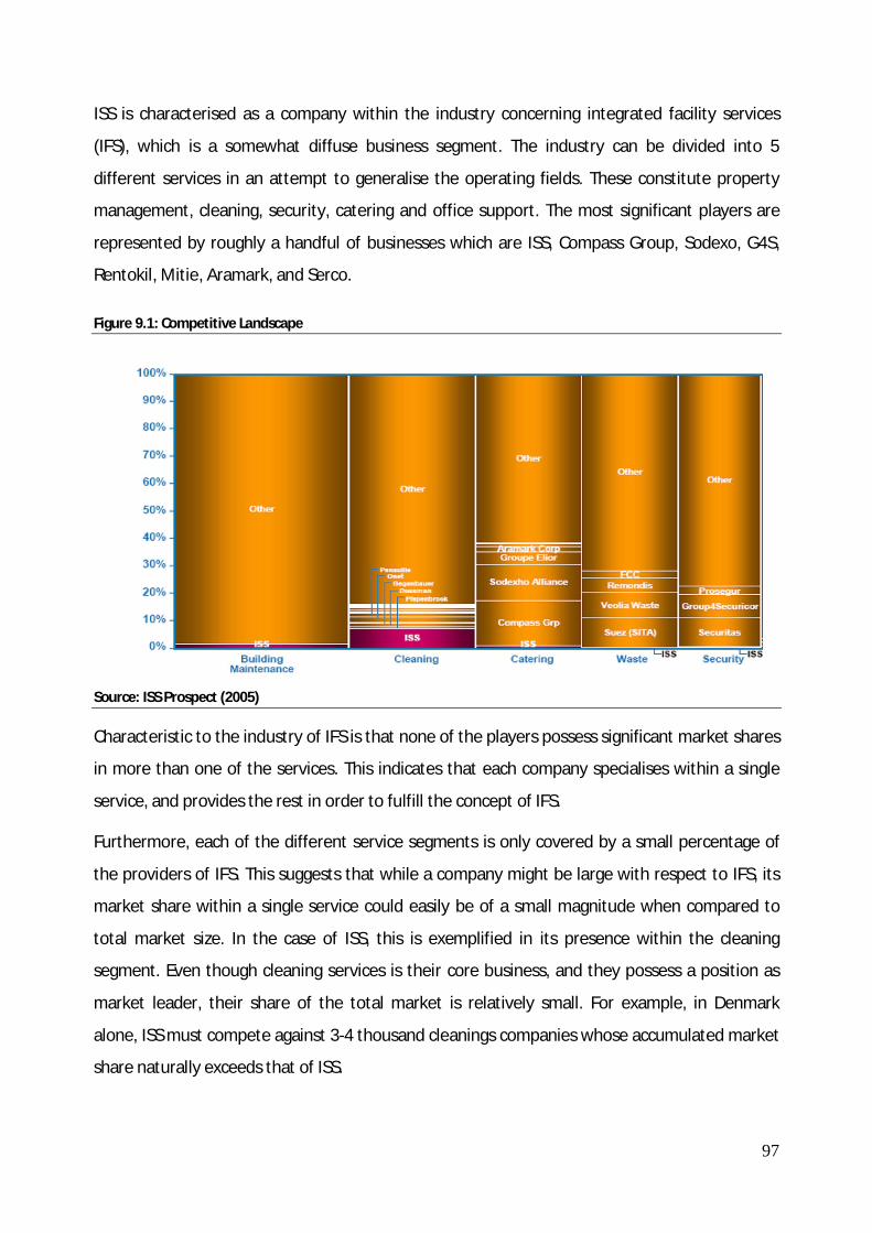
97

ISS is characterised as a company within the industry concerning integrated facility services

(IFS), which is a somewhat diffuse business segment. The industry can be divided into 5

different services in an attempt to generalise the operating fields. These constitute property

management, cleaning, security, catering and office support. The most significant players are

represented by roughly a handful of businesses which are ISS, Compass Group, Sodexo, G4S,

Rentokil, Mitie, Aramark, and Serco.

Figure 9.1: Competitive Landscape

Source: ISS Prospect (2005)

Characteristic to the industry of IFS is that none of the players possess significant market shares

in more than one of the services. This indicates that each company specialises within a single

service, and provides the rest in order to fulfill the concept of IFS.

Furthermore, each of the different service segments is only covered by a small percentage of

the providers of IFS. This suggests that while a company might be large with respect to IFS, its

market share within a single service could easily be of a small magnitude when compared to

total market size. In the case of ISS, this is exemplified in its presence within the cleaning

segment. Even though cleaning services is their core business, and they possess a position as

market leader, their share of the total market is relatively small. For example, in Denmark

alone, ISS must compete against 3-4 thousand cleanings companies whose accumulated market

share naturally exceeds that of ISS.

98

In the process of identifying suitable peers, some of the above mentioned competitors were

initially excluded due to operations within areas other than IFS. Consequently, the effects of

these additional operations would be reflected in the obtained multiples - resulting in an

incorrect foundation. Furthermore, some have been excluded as a consequence of not being

listed. This is inevitably a requirement when peers are utilised with respect to obtaining trade

multiples.

To obtain the most accurate peer group among the remaining companies, the peers selected

should carry similar characteristics to those of ISS. In this respect, the characteristics identified

as being most influential are growth, strategic position, and operational risk (as described in

section 8.1.1). Analysis performed on each individual competitor reveals that Sodexo, Compass

Group, and G4S (formerly Group 4 Securicor) possess similar characteristics to those of ISS.

Firstly, in recent years, growth rates have resembled each other - primarily achieved through

aggressive acquisition strategies.

Secondly, all companies possess a dominating strategic position within their respective field of

core operations, as illustrated in figure 9.1.

Finally, even though the services within their different core businesses are not alike, the

operational risk associated is fairly assumed similar, as the industries in question carry relatively

consistent characteristics. The companies alike provide services through long term contractual

agreements which ensure relatively stable earnings.

We recognise the fact that three companies constituting a peer group analysis could be

considered a relatively small foundation. However, emphasis on the correctness of peers is

preferred as opposed to the share basis of comparison.

9.3. ESTIMATION OF ENTERPRISE VALUE

As described in the theoretical part of the paper, the estimation of the enterprise value of ISS

will be performed on the basis of a multiples analysis. The basic idea is to find the average

trading multiple of the peer group compared to ISS at the time of the takeover. This returns a

ratio at which ISS was traded, compared to its peer group. The multiple ratio is then applied to

year end 2008 multiples of the peers - providing a fair estimate of the current ISS multiple.

The analysis is initiated by obtaining market capitalisation and net debt of the peer group and

ISS before it was de-listed. The enterprise values are then divided by the corresponding EBITDA

99

of the same period, which yields the trading multiple EV/EBITDA. These results appear in table

9.2.

Table 9.2: EV/EBITDA Multiples

Source: Own construction

Trading multiples obtained at the day of the buyout, are based on realised 2004 EBITDA, while

market cap are actual figures of the current time and net debt is adjusted9 for the purpose. On

the basis of these figures an EV/EBITDA multiple of the ISS transaction is 10.5x.

When the leverage buyout of ISS was performed in March 2005, the acquisition was completed

at a price in which a considerable premium of 31.3 % was included. This premium reflected

expectations of increased earnings contained in concentrated ownership. We assume that,

during the four years in which ISS has been de-listed, these opportunities have been fulfilled

and are, thus, contained in the current EBITDA. Consequently, the premium paid should not be

reflected in the current multiple as the higher enterprise value is now expressed through the

increased EBITDA. This implies that the multiple of 10.5x should be cleansed of the premium

when applied as the foundation on which the multiple ratio is based. Calculating market cap

less premium and solving for the adjusted multiple yields 8.6x. This provides the multiple ratio

8.6/8.0 = 1.075 of which ISS traded to its peer group at the time of the takeover.

In our peer group analysis we carefully selected comparable companies which we assume carry

the same risk and similar growth expectations as that of ISS. The assumption of “carbon copies”

allows us to transfer the multiple ratio obtained from the day of the buyout directly, up to

9 The method of adjusting the debt is provided in section 9.4

Multiples

Company EV/EBITDA 04

EV/EBITDA 29/03/2005

EV/EBITDA 05

EV/EBITDA 06

EV/EBITDA 07

EV/EBITDA 08

EV/EBITDA 31/03/2009

G4S 9,1 9,3 8,2 8,5 12,6 10,5 5,7Sodexo 6,1 6,9 8,7 10,5 8,2 7,6 6,3

Compass 7,5 7,7 7,6 10,5 9,4 8,5 5,9Average 7,6 8,0 8,2 9,8 10,1 8,9 6,0

ISS 7,6 10,5ISS Adjusted 7,6 8,6 8.0

100

today. Applying the multiple ratio to the average peer group EV/EBITDA multiple, based on

2008 figures, results in an estimated ISS multiple of 9.6x10.

However, the general assumption is that the stock market is traded on expectations for the

future. An approach built on expectations for EBITDA 09 of the peers, returns an estimated ISS

multiple of 6.5x. In light of the unpredictable market conditions following the credit crisis, the

uncertainty surrounding expectations to 2009 is, in our assessment, too great to be fully relied

upon. It is evident that investors will not fully reward the expectations of an increased EBITDA

in conditions of high uncertainty.

Based on the considerations of uncertainty, we assume that an equally weighted average of the

two estimates, provided by realised EBITDA 08 and expected EBITDA 09, satisfies a true and fair

estimate of the actual ISS multiple today. This results in a final ISS multiple of 8.0x EV/EBITDA.

In the perspective of current buyout activity, the achievement of a trading multiple of 8.0x

seems rather realistic. In section 5.2, we provided evidence that current leverage buyouts are

on average executed at 7.9x EV/EBITDA.

With the given multiple we are now able to find the estimated enterprise value of ISS end year

2008. This is achieved simply by multiplying EBITDA with EV/EBITDA, which returns an

estimated enterprise value of ISS = 4936.511 * 8.0 = DKK 39.492 billion.

9.4. ESTIMATION OF VOLATILITY

When estimating the volatility of the enterprise value of ISS, peer group characteristic is once

again utilised. The following calculations appear in full in appendix B and C which are based on

figures provided by Factset (formerly JCF).

Estimation of volatility is initiated by calculating the enterprise value of each company on a

daily basis beginning from 01/01/2004 to 31/12/2008. In the case of ISS the enterprise is

derived until it was de-listed as of 29/03/2005. In order to perform these calculations we need

to obtain daily share values, shares outstanding and net debt. While share values are easily

obtained, shares outstanding and net debt are not widely available on a daily basis. In an

attempt to circumvent this problem, shares outstanding and net debt is obtained on a yearly

basis. To create an evolving development throughout each year, the difference from year to

10 8.9x * 1.075 = 9.6x 11 Since we have applied an equally weighted EBITDA to the peers we utilize an equally weighted EBITDA of ISS as well. Realized EBITDA 2008 was 4837 and expectations to EBITDA in 2009 are 5036.

101

year is divided by the number of trade days in between. This creates a fraction which is

added/subtracted for each day moving forward to get the day by day evolution. Although

shares outstanding and net debtdo not evolve at the exact same fraction consistently during

each year, we assume this approach satisfies the actual evolution within each company.

On the basis of the estimated parameters above, enterprise values are calculated on a daily

basis. The enterprise values are then treated as returns in the equally weighted moving average

approach, where they are taken as inputs to volatility estimation. We have chosen to measure

the annualised historical volatility for each specific day based on an average of 2 month, 1

month, 2 weeks, and 1 week. In order to estimate which of the four time frames provide the

best fit, we perform a Root mean Squared Error (RMSE) analysis. This reveals how well the

historical volatility predicts the excess change the following day. The period providing the

smallest result is the best measure.

Table 9.3: Root Mean Squared Average

Source: Own Calculations

We find that RMSE differs between each company within the peer group. However, this has no

influence when calculating the average peer group volatility, as it is only an expression of the

best measure. The standard deviations obtained from differentiating time frames across the

companies are not affected.

We now pick the volatilities at the two given dates of each company corresponding with the

time frame providing the best fit. The volatility of ISS is compared to the peer group on the day

before its de-listing. The ratio between ISS and its peers is forwarded to the average volatility of

the peer group as of 31/12/2008. This returns the estimated volatility of ISS at 0.22.

Root Mean Squared Average

Date 29-03-2005 31-12-2008

Time frame 2 month 1 month 2 week 1 week 2 month 1 month 2 week 1 week

G4S 0,0002849 0,0003164 0,0003349 0,0003492 0,0003715 0,0003741 0,0003787 0,0003812

Sodexo 0,0005559 0,0005425 0,0005497 0,0005614 0,0007086 0,0006993 0,0007041 0,0007328

Compass 0,0027193 0,0026540 0,0008454 0,0011655 0,0014912 0,0014935 0,0006815 0,0008309

ISS 0,0001279 0,0001280 0,0001290 0,0001344

102

Table 9.4: Volatility

Source: Own Calculations

9.5. DETERMINATION OF BANKRUPTCY COSTS, TAX, AND RISK FREE RATE

We have chosen to direct our focus on empirical studies performed on highly leveraged firms

due to the high degree of uncertainty and complexity in estimating the fraction lost to

bankruptcy costs. Studies by Bris, Welch and Zhu (2004) estimates that direct costs amount to

9.5% while Andrade and Kaplan (1998) estimates the indirect cost of financial distress to be

somewhere between 10 to 20 % of firm value. By adding these findings the total bankruptcy

costs seem to be in the area of 20 - 30 %.

Turning our attention towards more industry specific recovery rates a Credit Suisse rapport

(Blau et al., 2008) states that the recovery rate of leveraged loans in the service sector have

been 49.5 percent in LTM September 2008. Comparing a fraction lost to bankruptcy costs of

50.5 percent with the findings of the empirical studies reveals relatively large inconsistencies.

However, considering the characteristics of ISS and the industry in which it operates it seems

reasonable that the service sector will be affected more severely than the average industry

findings in the empirical studies. Consequently, we have chosen to rely on the industry specific

recovery rate which yields a fraction lost to bankruptcy costs at 50.5 percent.

The tax rate applied in the model is the effective tax rate calculated from the annual report of

2008 of ISS which is 15.5 %12.

The risk free rate is obtained from a Danish government bond with a maturity of 10 years. As of

31/12/2008, the effective rate was 3.4 percent (Nationalbanken, 2009).

12 This is achieved by dividing taxes paid with pre-tax profit.

Volatility

Date 29-03-2005 31-12-2008

G4S 0,23 0,30

Sodexo 0,21 0,38

Compass 0,10 0,32

ISS 0,12 0,22

103


In the estimation of the enterprise value we found the leveraged buyout transaction of ISS was

performed at an EV/EBITDA multiple of 8.6x excluding the premium paid. Utilisation of

comparative multiples determine the present ISS multiple at 8.0x. Effectively, the present

enterprise value of ISS is DKK 39.492 million.

The volatility estimation was similarly performed on the basis of peer group comparison.

Applying the EWMA approach we found the present volatility of ISS to be 0.22.

The fraction lost to bankruptcy costs is determined at 0.505 based on the historical industry

specific recovery rate of leveraged buyouts. Finally, we found the effective tax rate of ISS to be

15.5 percent, while the risk free interest rate was determined at 3.4 percent.

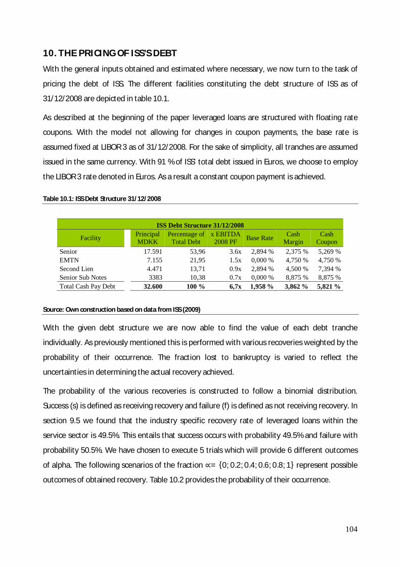
104

10. THE PRICING OF ISS’S DEBT

With the general inputs obtained and estimated where necessary, we now turn to the task of

pricing the debt of ISS. The different facilities constituting the debt structure of ISS as of

31/12/2008 are depicted in table 10.1.

As described at the beginning of the paper leveraged loans are structured with floating rate

coupons. With the model not allowing for changes in coupon payments, the base rate is

assumed fixed at LIBOR 3 as of 31/12/2008. For the sake of simplicity, all tranches are assumed

issued in the same currency. With 91 % of ISS’ total debt issued in Euros, we choose to employ

the LIBOR 3 rate denoted in Euros. As a result a constant coupon payment is achieved.

Table 10.1: ISS Debt Structure 31/12/2008

ISS Debt Structure 31/12/2008

Facility

Principal MDKK

Percentage of Total Debt

x EBITDA 2008 PF Base Rate Cash

Margin Cash

Coupon Senior 17.591 53,96 3.6x 2,894 % 2,375 % 5,269 % EMTN 7.155 21,95 1.5x 0,000 % 4,750 % 4,750 % Second Lien 4.471 13,71 0.9x 2,894 % 4,500 % 7,394 % Senior Sub Notes 3383 10,38 0.7x 0,000 % 8,875 % 8,875 % Total Cash Pay Debt 32.600 100 % 6,7x 1,958 % 3,862 % 5,821 %

Source: Own construction based on data from ISS (2009)

With the given debt structure we are now able to find the value of each debt tranche

individually. As previously mentioned this is performed with various recoveries weighted by the

probability of their occurrence. The fraction lost to bankruptcy is varied to reflect the

uncertainties in determining the actual recovery achieved.

The probability of the various recoveries is constructed to follow a binomial distribution.

Success (s) is defined as receiving recovery and failure (f) is defined as not receiving recovery. In

section 9.5 we found that the industry specific recovery rate of leveraged loans within the

service sector is 49.5%. This entails that success occurs with probability 49.5% and failure with

probability 50.5%. We have chosen to execute 5 trials which will provide 6 different outcomes

of alpha. The following scenarios of the fraction ∝= {0; 0.2; 0.4; 0.6; 0.8; 1} represent possible

outcomes of obtained recovery. Table 10.2 provides the probability of their occurrence.

105

Table 10.2: Probability Distribution

Source: Own Calculations (See Appendix D)

The binomial probability distribution in figure 10.3, displays the probability of all possible

scenarios of alpha occurring.

Figure 10.3: Binomial Probability Distribution


The approach incorporates an element of uncertainty of alpha and thereby avoids the

deterministic drawbacks consisting of pre-determination of recovery. From the theoretical

framework, we know that the individual debt value consists of two parts: (1) The discounted

return on the continuous compounded coupons until bankruptcy occurs, and (2) The

discounted return on the obtained recovery. We have chosen to let 푉 remain fixed in order

not to affect the determination of when bankruptcy is declared, expressed by . This

α 0 0,2 0,4 0,6 0,8 1u sssss ssssf sssff ssfff sffff fffff

P(u) 0,0297 0,0303 0,0309 0,0316 0,0322 0,0328X 1 5 10 10 5 1

P(X) 0,0297 0,1516 0,3093 0,3156 0,1610 0,0328

Binomial Distribution

0

0,05

0,1

0,15

0,2

0,25

0,3

0,35

0 0,2 0,4 0,6 0,8 1

Prob

abili

ty

Fraction (α)

106

implies that the former remains constant at all times, while the latter is affected by the

different values of α.

We are now able to initiate the model calculations. The different parameters required in the

model framework are listed in table 10.4.

Table 10.4: Model Inputs


It is worth noting that the fraction lost to bankruptcy at 50.5 percent works as our foundation in

determining the possibilities of achieving various recoveries.

With the inputs employed in the model we obtain the price of ISS’s debt in the different

scenarios of 훼. These are provided in the table 10.5.

Table 10.5: ISS Debt Prices in Various Scenarios of Alpha

Source: Own Calculations (See Appendix E)

It appears how the priority of the different tranches is in correspondence with their respective

claims to achieved recovery. This is for example seen in the senior subordinated tranche which

is affected as soon as alpha is increased from 0 to 0.1. The tranche is precluded from receiving

recovery as alpha increases to 0.2. At this point the second lien tranche becomes affected

which corresponds with the size of the senior subordinated tranche and the two tranches

individual placement in the capital structure. The price of the senior tranche is not affected

until the fraction lost to bankruptcy costs exceeds 50 percent.

39.4920.2200.5050.1150.0340.029

Riskless Rate (r)

Estimated and obtained valuesEnterprise Value (V)Volatility (σ)Fraction lost to Bankruptcy (α)Tax Rate (τ)

Constant Base Rate (LIBOR 3)

FacilityPrincipal MDKK

Price when α = 0

Price when α = 0.1

Price when α = 0.2

Price when α = 0.3

Price when α = 0.4

Price when α = 0.5

Price when α = 0.6

Price when α = 0.7

Price when α = 0.8

Price when α = 0.9

Price when α = 1.0

Senior 54% 112,98 112,98 112,98 112,98 112,98 107,38 93,22 79,07 64,92 50,76 36,61EMTN 21% 109,38 109,38 109,38 88,82 54,02 33,00 33,00 33,00 33,00 33,00 33,00Second Lien 14% 127,75 127,75 74,16 51,37 51,37 51,37 51,37 51,37 51,37 51,37 51,37Senior Sub 11% 138,04 64,44 61,66 61,66 61,66 61,66 61,66 61,66 61,66 61,66 61,66

Price Calculation in Various Scenarios

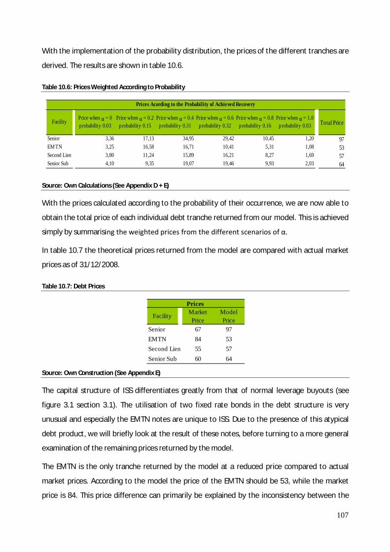
107

With the implementation of the probability distribution, the prices of the different tranches are

derived. The results are shown in table 10.6.

Table 10.6: Prices Weighted According to Probability

Source: Own Calculations (See Appendix D + E)

With the prices calculated according to the probability of their occurrence, we are now able to

obtain the total price of each individual debt tranche returned from our model. This is achieved

simply by summarising the weighted prices from the different scenarios of α.

In table 10.7 the theoretical prices returned from the model are compared with actual market

prices as of 31/12/2008.

Table 10.7: Debt Prices

Source: Own Construction (See Appendix E)

The capital structure of ISS differentiates greatly from that of normal leverage buyouts (see

figure 3.1 section 3.1). The utilisation of two fixed rate bonds in the debt structure is very

unusual and especially the EMTN notes are unique to ISS. Due to the presence of this atypical

debt product, we will briefly look at the result of these notes, before turning to a more general

examination of the remaining prices returned by the model.

The EMTN is the only tranche returned by the model at a reduced price compared to actual

market prices. According to the model the price of the EMTN should be 53, while the market

price is 84. This price difference can primarily be explained by the inconsistency between the

FacilityPrice when α = 0 probability 0.03

Price when α = 0.2 probability 0.15




Price when α = 1.0 probability 0.03 Total Price

Senior 3,36 17,13 34,95 29,42 10,45 1,20 97EM TN 3,25 16,58 16,71 10,41 5,31 1,08 53Second Lien 3,80 11,24 15,89 16,21 8,27 1,69 57Senior Sub 4,10 9,35 19,07 19,46 9,93 2,03 64

Prices Acording to the Probability of Achieved Recovery

Facility Market Price

Model Price

Senior 67 97EMTN 84 53Second Lien 55 57Senior Sub 60 64

Prices

108

model assumption of perpetual debt and the actual maturity of the tranche in 2010. From a

theoretical perspective, the tranche is priced as all the other tranches, namely as the

discounted return on the continuous compounded coupons until bankruptcy and the

discounted return on the obtained recovery. However, with a repayment in the near future,

market participants almost exclusively value debt according to the probability of receiving the

full principal at maturity. In the case of ISS where the EMTN constitutes a minor pat of the

capital structure, the risk of ISS not being able to refinance the tranche is low, and therefore is

it is only natural that the price goes up. Consequently, the price on the EMTN returned from the

model is much lower than the price observed in the market (Christiansen, 2009).

With the exception of the somewhat unusual EMTN notes, we will, in the following section,

attempt to provide an explanation for the general inconsistencies between actual market prices

and the prices returned by the model. These are analysed from two different approaches: (1)

Practical and (2) Theoretical. The practical point of view identifies model specific sources

including input errors which might pollute the returned results, while the theoretical point of

view explains potential sources for any inconsistencies not model related.

10.1 PRACTICAL FOUNDATION FOR INCONSISTENCIES

The construction of the model relies on several assumptions to be satisfied, which are not in

precise correspondence with actual market conditions. In the following, we will pinpoint some

of the most influential ones causing price inconsistencies.

One of the factors determining the occurrence of bankruptcy is the size of coupon payments. In

the theoretical approach coupon payments are assumed fixed, but the senior debt and second

lien of ISS are actually based on floating rate coupons. This implies that fluctuations in coupon

payments will be neglected by the model, and consequently the determined occurrence of

bankruptcy could become incorrect. In defense of the model, it should be noted that leveraged

companies to a hedge substantially against their exposure to LIBOR. Nevertheless, the

treatment of floating rate coupons as fixed can be a contributing factor in deviations from

observed prices.

Another assumption of the model is time independence which implies that debt is issued as

perpetual debt. In theory this seems to be a valid assumption as leveraged loans are issued with

long term maturities. However, this approach excludes the possibility of an early repayment.

109

The discrepancy which arises in this respect is that leveraged loans are, in general, issued as

callable debt. This necessitate that any prices more than insignificantly above par are highly

unlikely to occur. Had the obtained recovery rate been slightly higher in the case of ISS, this

discrepancy would have been displayed in the pricing of senior debt. Effectively, the theoretical

price of the senior tranche would have been above par.

According to Torben Skødeberg, market valuation of leveraged loans is primarily based on a

thorough examination of the cash flows generated by the underlying company. This is due to

the fact that the cash flows are the primary determinant of bankruptcy declaration. In this way,

it is important to ensure that the cash flows generated by the firm are sufficient to cover the

coupon payments until maturity. The model, in contrast, assumes that the reach of a pre-

determined lower value of the enterprise will trigger bankruptcy. Although there is a high

correlation between cash flows and enterprise value, the two approaches can return different

determinations of when bankruptcy occurs. This implies that the comparison of theoretical and

market prices relies on two different valuation methods with respect to bankruptcy

determination.

Finally, it is worth noting that the capital structure of ISS is not a plain vanilla example of a

leveraged buyout. However, the model treats all tranches as if they were issued as leveraged

loans. This can obviously lead to pricing errors with respect to the debt products, besides

leveraged loans. Beyond the previously mentioned EMTN tranche, this implies that the

returned theoretical price of the senior subordinated tranche might be misleading.

Several of the input variables are based on estimations which imply that inconsistencies can be

caused directly from errors in the performances of these. Performing stress tests will reveal to

which degree flaws in the different estimations influence the total outcome. We have chosen to

perform stress tests on the variables: volatility, enterprise value and the fraction lost to

bankruptcy costs. The results of which are presented in table 10.8.

110

Table 10.8: Stress Test

Source: Own Calculations (See Appendix F)

The stress tests performed cover deviations from the estimated values in a range of +/- 10

percent. This provides an overview of the affects of changes in the different input variables to

the individual tranches.

Basically, increasing the volatility lowers the value of 푋 which increases the last term of the

model, . This implies that the more volatile the enterprise value is, the larger becomes

the determinant of when bankruptcy is declared. Naturally, these affects are reverse when

decreasing the volatility. As a result, an increase in the volatility is equivalent to a more

imminent reach of 푉 . This will affect the prices negatively as total coupon payments are

decreased. The occurrence of changes in volatility has a fairly large impact on the lower

tranches whereas the most senior tranche hardly is affected. This is due to the priority of debt

which implies that the lower tranches are more dependent on generating cash flows while alive

compared to the senior tranche. The latter will collect the most substantial part of the returned

recovery and therefore does not suffer the same exposure as to when 푉 reached.

Of the three input variables, changes applied in the enterprise value prove to affect the prices

of the debt tranches most significantly. The effects are the least obvious in the most senior

tranche, while the two lower tranches in particular are influenced. There reasons are the same

as those provided with respect to 푉 when changing the volatility. However, this time 푉

remains fixed while 푉 either approaches or moves away. In addition, there exist a natural

relationship between the changes applied and the effects on the prices. However, it's worth

noting how negative changes entail stronger affects to the price than positive ones do.

Lowering the enterprise value implies that 푉 → 푉 which indicates that bankruptcy is

becoming more possible to occur. As such, the affects of the changes highly resemble those,

one would expect to see in the real world.

Volatility EV Alpha Volatility EV Alpha Volatility EV Alpha Volatility EV Alpha Volatility EV AlphaSenior 100 87 100 98 92 98 97 97 97 95 100 94 94 104 92EMTN 59 40 59 56 47 56 53 53 53 51 59 51 49 64 48Second Lien 67 32 60 62 45 58 57 57 57 53 68 56 49 77 55Senior Sub 76 32 65 70 49 65 64 64 64 59 77 63 54 89 63

Stress Test

Facility-10% -5% 0% 5% 10%

111

The affects on prices when changing alpha are of a smaller magnitude compared to those of the

other two variables. However, when exposed to changes alpha proves to be the only variable

which affects the EMTN tranche more severely than any of the other tranches. With the given

capital structure and the base case fraction this is in perfect compliance with what is to be

expected. The reason being when increasing alpha the weight of the scenarios dominated by

failure will increase while lowering alpha increase the influence of the success scenarios.

10.2. THEORETICAL FOUNDATION FOR INCONSISTENCIES

The model returns prices which in general are higher than actual market prices - disregarding

the obvious flaw appearing in the low price of the unique EMTN. Consequently, we will attempt

to locate possible issues which from a theoretical point of view can explain some of the

inconsistencies not related to the model.

Even though the leveraged loan market has been strongly influenced by an increased

institutional investor base, it is worth remembering that the European leveraged loan market is

still affected by banks possessing a substantial market share. Leveraged loans are to some

extend still treated as bank products, and therefore not yet fully driven by capital market forces

as oppose to the more traditional bond market. The advantages of possessing the role as

relationship bank calls for speculations concerning whether banks have been willing to issue

the loans at reduced margins in order to acquire this role. The existence of loans not priced in

complete correspondence with actual returns, implies a possible contortion of leveraged loan

prices.

In this relation, bank credit has during the last decade evolved from the approach of the

traditional relationship banking towards originate-to-distribute. In particular, the bull-run days

provided banks the opportunity to originate loans, earn the fees, and then sell the loans to

other investors. Studies provided by Berndt and Gupta (2008) provide evidence of a risk-

adjusted underperformance of these loans of approximately 10 percent compared to other

bank loans. In general, two reasons for this underperformance exist. These are adverse

selection and moral hazard. The first explanation deals with banks’ superior information about

the credit quality of their loans, which gives rise to concerns about adverse selection. The

underperformance of the loans could be explained by banks originating and, subsequently,

selling bad loans based on unobservable private information. Secondly, the increasing

112

outdistancing to traditional relationship banking meant a severance of the bank-borrower

relationship. In the absence of the discipline of bank monitoring, borrowers were provided the

opportunity to undertake suboptimal operating and investment decisions. Effectively, the

syndication fee structure combined with a high degree of information asymmetry calls for

speculations of adverse selection and moral hazard problems within the leveraged loan market.

Based on the structure of remuneration to the CLO manager indications of a possible principal

agent problem seem present. In section 6.2.2 we found that the lack of sub-fees in relation to a

potential breach of the CCC-bucket may result in the CLO manager behaving opportunistically

as he is left no incentive to do otherwise. Effectively, the preclusion of the substantial sub fees

implies that the CLO manager would trigger insolvency which is absolutely not in the interest of

the investors. However, if he cannot maintain a minimum service platform this will result in an

inability to comply with operational service requirements and in the long run remain solvent.

10.3 RECAPITULATION

When comparing theoretical prices to actual market prices, we find that the model in general

prices the loans higher – setting aside the inconsistencies concerning EMTN.

The theoretical prices of the two most junior tranches are only marginal above those observed

in the market. This causes us to believe that the existing differences might be based on one of

the identified practical factors found in section 10.1. Especially the results of the stress tests

suggest that minor flaws in the estimation of input variables can explain the observed

differences. We have identified volatility and enterprise value as the most likely estimated

inputs to be polluted by flaws. We find that less than a 5% decrease in enterprise value would

result in theoretical prices similar to market prices. Likewise, an increase of less than 5 percent

in volatility returns compliant prices.

The model prices the senior tranche highly above the observed market prices. Given the

magnitude of the deviation it seems unlikely that this is solely caused by practical or theoretical

factors. In compliance with the knowledge obtained in the market analysis (see part 3) it

appears that a liquidity premium currently is being offered in the market with respect to senior

secured debt.

113

Assuming that the theoretical price of the senior tranche reflects the actual conditions of ISS,

we have chosen to perform a calibration of the fraction lost to bankruptcy costs. This illustrates

at which fraction actual market prices are traded. The results are provided in table 10.9.

Table 10.9: Calibration

Source: Own Calculations (See Appendix G)

We concentrate on the senior secured tranche in our attempt to identify at which fraction lost

to bankruptcy costs the loans are traded. This is because this tranche seems to be the only one

offering a liquidity premium.

It appears that increasing the expected fraction highly narrows the existing gap between

theoretical and market prices. With a fraction lost to bankruptcy costs of 78 percent the

theoretical price reaches the price observed in the market. This implies that leveraged loans are

currently traded with an implied recovery rate of merely 22 percent. In addition, this provides

the answer as to why no liquidity premium is offered in the two most junior tranches. The

implied recovery rate at which leveraged loans are currently being traded only affects the

prices of the junior tranches insignificantly. This is due to their placement in the capital

structure. With the actual recovery rate of 49.5 percent they are both almost entirely precluded

from receiving recovery in the event of bankruptcy. Therefore a decrease in the implied

recovery becomes without influence to the pricing of these tranches.

Effectively, we find that potential investors of senior secured leveraged loans are currently

being offered a fairly substantial liquidity premium. This is tantamount to senior leveraged loan

prices not currently reflecting the actual conditions of leveraged buyouts.

50% 60% 70% 78% 80%

Senior 97 88 77 67 64 67EMTN 53 44 38 35 35 84Second Lien 57 54 52 52 52 55Senior Sub 64 62 62 62 62 60

FacilityCalibration of Fraction lost to Bankruptcy Cost Market

Price

114

11. CONCLUSION

In the final chapter of the thesis, the main findings identified throughout the analysis will be

drawn together in a conclusion. In compliance with the structure of the thesis, this is performed

through a systematic assessment of the five analyses which finally leads to an answer of the

main research question proposed in the problem statement.

The first part of the thesis has provided the reader with an understanding of the most

fundamental characteristics of the leveraged loan market. Typically leveraged loans are issued

by companies involved in leveraged buyouts. One of the main characteristics differentiating

leveraged loans from more traditional high yield debt products is the way they are launched to

the market. Instead of entering a series of bilateral arrangements with each bank, a group of

banks share the same loan agreement. In this way private equity funds have been able to

access larger pools of funding than otherwise available. Likewise, the syndicated loan market

offers several advantages to banks according to their role in the syndicate. Especially the

mandate as lead arranger became attractive due to recent years' pleasant market conditions.

Acting more like investment banks, the battle of winning the mandate became more intense,

resulting in increasingly aggressive loan structures. Consequently, a moral hazard problem

arose between lead arrangers and other loan participants.

Looking at a typical capital structure of a leveraged buyout company it is apparent that it

consists of a wide range of different debt products. According to their priority, the most

common leveraged loans appear within the categories of senior, second lien and subordinated

debt. Denoted as either first or second lien, the vast majority of loans are senior secured

floating rate papers. Mezzanine loans are ranked as subordinated debt and are a direct

alternative to high yield bonds. In consequence of being a highly leveraged company the issuers

are restricted by comprehensive covenant packages which state how loose they can operate

and carry themselves financially.

The second part of the thesis has introduced the reader to the fundamental CLO structure. In

general, a CLO is a special purpose vehicle established to hold and manage a diversified pool of

leveraged loans. To finance the purchase of these loans, the CLO issues a series of rated notes

which are tranched according to priority. Created as an arbitrage vehicle the CLO generates

equity returns through the issuance of debt several times its equity contribution. The utilisation

of various credit enhancement techniques mitigates the risk associated with default in the

115

collateral pool and ensures that certain target ratings of the specific notes are achieved. Most

remarkable in this relation is the payment waterfall which dictates the priority of payments

accruing to investors of different tranches. This ensures that the claims of the higher rated

tranches to interest and principal proceeds are protected. The latter implies that increasingly

higher levels of subordinated capital provide protection against losses in the collateral pool.

Effectively, the CLO structure enables the issuance of tranches with different interest rates and

credit ratings. This has allowed for investments in leveraged loans to achieve investment-grade

ratings which entailed that institutional investors could enter the leveraged loan market as the

solvency burden associated with the lower rated leveraged loans was mitigated. Furthermore,

institutional investors were offered the opportunity to invest in diversified portfolios of

leveraged loans managed by experienced market participants. This made their limited expertise

within the area redundant. From the perspective of banks, the CLO structure has provided

them the opportunity to achieve off-balance financing while simultaneously generating fees

from servicing the loans and remaining the corporate relationship bank.

Through an in-depth analysis of the European primary and the secondary leveraged loan

market, it is clear that the increased institutional investor base have had major impacts on the

evolution of the leveraged loan market. In the years preceding the credit crisis, the hyper liquid

market conditions were attributed to a rapidly increasing institutional investor attention. Yet,

besides stimulating the leveraged loan market in the bull-run the institutional investors also

highly contributed to its total collapse.

The primary leveraged loan market has clearly been afflicted by the entrance of the credit crisis.

The volume of loan issuance has abruptly stalled and previous years' hyper liquid market

conditions seem far away. The structures of the few new transactions have improved

significantly. First of all leverage has gone down as a result of increasing equity contributions.

As a consequence purchase price multiples have fallen. Furthermore, the former years'

increasing complex debt structures have changed to more transparent and classic

senior/mezzanine capital structures. Finally, the shrunken investor base has forced spreads to

rise.

Since the onset of the credit crisis in summer 2007, the secondary loan market has gone

through a total meltdown and experienced a longer period of historically negative returns. A

comprehensive deleveraging process among hedge funds and market value CLOs lead to a

116

vicious circle of forced selling and falling prices. Such technical factors affecting the market

were later substituted with fundamental difficulties concurrently with the recession becoming

ever more real. In a risk adverse world, filled with distressed investors, outlooks of rising default

rates and low recovery rates pushed the market further in its knees. Starting above par during

the summer 2007, the ELLI Index ended below 60 at end year 2008.

In the fourth part of the thesis the reader has been provided a thorough exposition of the

theoretical framework for pricing corporate debt when tranched according to priority. The

derivation of the model was initiated on the basis of theoretical work provided by Merton,

Black & Scholes and Lando. This provided a theoretical framework for pricing sequentially

tranched corporate debt when issued as zero-coupon bonds. With leveraged loans primarily

issued as coupon bonds, we turned to the pricing theory provided by Leland. The original model

of Leland for pricing corporate debt issued as coupon bonds was derived. Afterwards we

extended the model to handle prioritised debt. The extension proved to accentuate the

deterministic drawbacks of the model. In order to circumvent these, we found that the

implementation of a binomial distribution with respect to the fraction lost to bankruptcy costs

solved the problem. This enabled the model to return theoretical prices comparable with actual

market prices.

The extensive knowledge obtained, regarding the leveraged loan market, enabled an

examination of the theoretical results. The findings of our model implementation and the

current conditions of the leveraged loan market form the foundation for a qualified answer to

the main research question.

Can market prices of leveraged loans be supported from a theoretical point of view?

We find that no precise answer can be provided based on the finding throughout this thesis.

The results related to the individual tranches are of an ambiguous character which makes a

general answer to the main research question impossible.

The theoretical price of the EMTN tranche is affected by the model assumption of time

independence which excludes this tranche as a foundation for comparison with actual market

prices.

Generally seen, the market prices of the two most junior tranches appear to be supported from

a theoretical point of view. We find that practical and theoretical issues might explain some of

117

the observed deviations between model and market prices identified. In particular, the results

of the stress tests suggest that minor estimation flaws with respect to enterprise value and

volatility could be present.

The theoretical obtained price of the senior tranche suggests that senior secured leveraged

loans are currently traded at market prices which are too low. The difference between

observed and theoretical prices of the senior tranche in the ISS case is more than 40 percent.

This implies that neither theoretical nor practical factors are likely to explain this gap in prices.

With the current condition of the leveraged loan market we believe that a liquidity premium

reflects the existing difference.

These indications let to a calibration of the fraction lost to bankruptcy costs. The finding of

which indicated an implied recovery rate of merely 22 percent is utilised in the market. In

compliance with the knowledge obtained in the performed market analysis, this entails that a

liquidity premium is being offered to potential senior secured leveraged loan investors. As a

result of the credit crisis, the leveraged loan market has experienced a longer period of forced

selling. In particular hedge funds and market value CLOs were heavily afflicted by a broader

credit system that was severely overextended. The forced deleveraging process among these

institutional investment vehicles, along with a rapidly contracting investor base, has created a

significant supply/demand imbalance in the market. Severely influenced by technical factors,

market prices of senior secured leveraged loans cannot be supported from a theoretical point

of view.

118

12. REFERENCE LIST

Ahluwalia R., Flanagan C., Wang M., Lamy D., Nachiappan N., Gupta R., Caldana D., Webb A. & Horsley R. (2009) CLO Overlap – Implications for loan technicals, resturcturings & relative value, J.P.Morgans, 12 February 2009 Barr A. (2007) Hedge funds try to hold back wave of investor redemptions November 28. 2007, Businessweek (MarketWatch), San Francisco URL: http://bx.businessweek.com/ Black F. & Scholes M. (1973) The Pricing of Options and Corporate Liabilities, Journal of Political Economy, Vol. 81, No. 3., May-Jun, 1973, pp. 637-659 Blau J., Chen M., Seweeney D. & Yung J. (2008) Leveraged Finance Strategy Update - Third Quarter 2008 Institutional Leverage Loan Default Review, Credit Suisse, 9 October 2009 Citigroup (2005) Leveraged Loan Handbook – A guide to the Corporate Loan Market, June 27, Citigroup Global Markets Ltd. Cummings R., Hampden-Turner M., Ciampichetti E. & Raja A. (2008) Why are so many equity investors now interested in leveraged loans?, Citigroup Global Markets Ltd., November 2008 Edward I. Altman, Corporate Financial Distress and Bankruptcy: Predict and Avoid Bankruptcy, Analyze and Invest in Distressed Debt, 3rd Edition, Wiley Finance, 2006 European High Yield Association, EHYA (2009) URL: http://www.ehya.com/ Viewed: 04.04.2009 Eyerman E. (2009) The Long March for European Leveraged Credit, FitchRatings, June 2009 Eyerman E., Mazzini P., De Angelis M., Makhan M., Volkmer M., Durand-Agbo C., Barker G., Porte A. & Conti P.A. (2009) The Long March – The Outlook for European Leveraged Credit, Europe Special Report, FitchRatings, 22 April 2009 Fabozzi F.J. & Kothari V. (2007) Securitization: The Tool of Financial Transformation, Yale ICF Working Paper No. 07-07 Gadanecz, B. (2004) The Syndicated Loan Market: Structure, Development and Implications, Bank for International Settlements (BIS), BIS Quarterly Review, December 2004 Gorton, G. & Souleles, N. (2005) Special Purpose Vehicles and Securitisation, Journal of Economic Litterateur, (Sep., 2005) ISS (2009) Investor presentation – Full year 2008 results, 28 February 2009 King M., Fenn J., Lorenzen H.P., Roy R., Hampden-Turner M., Foux M., Trampolsky E., Goves P., Shoup J.B (2009) Buy More Bonds, Credit Outlook 2009, US National Archives adapted by

119

CitiGroup, January 2009 Lando D. Credit Risk Modelling: Theory and Applications, Princeton University Press, 2004. Leland H. (1994) Corporate Debt Value, Bond Covenants and Optimal Capital Structure, Journal of Finance, Vol. 49, No. 4, (Sep., 1994), pp. 1213-1252 Leland H. (2006) Structural Models in Corporate Finance, Lecture 2: A New Structural Model, University of California, Berkeley, Revision 3, December 2006 Loan Market Association, LMA (2009) Guide to Syndicated Loans URL: http://www.loan-market-assoc.com/ Viewed: 03.04.2009 Loan Market Association, LMA (2009a) Guide to Syndicated Leveraged Finance URL: http://www.loan-market-assoc.com/ Viewed: 03.04.2009 Lucas D.J., Goodman L. & Fabozzi F.J. (2007) Collateralized Debt Obligations and Credit Risk Transfer, Yale ICF Working Paper No. 07-06 McGaiven R. (2009) From hero to villain: Leveraged market fights for survival, Leveraged Commentary & Data, Standard & Poor’s, January 2009 McGaiven R. (2009a) Inst’l investors face new frontiers amid credit crunch, Leveraged Commentary & Data, Standard & Poor’s, 2009 McGaiven R. & Yang R. (2009) A Primer for the European Syndicated Loan Market, Standard & Poor’s, We All Fall Down: Leveraged Lending Suffers Massive Contracting As Credit Crunch Bites, January 2009: New York McCLure B. (2006) A Clear Look At EBITDA , Forbes Media Inc. Merton, R.C. (1974) On the Pricing of Corporate Debt: The Risk Structure of Interest Rates, Journal of Finance, Vol. 29, No. 2, May 1974, pp. 449-470 Jensen C.N. (2008) A Great Buying Opportunity? The Absolute Return Partners LLP, March 2008 Plenborg T. & Petersen C. (2005) Regnskabsanalyse for beslutningstagere, 1st.ed., Thomson Plesner S. (2002) Structured Finance (1): Asset securitisation - ny arbejdsdeling i den finansielle formidling, Finans/Invest, No. 5. Plesner S. (2002a) Structured Finance (2): Collaterized debt obligations - struktureret gæld med giftigt bundfald, Finans/Invest, No. 6. Plenborg T. (2002), FSR – Fagligt nota tom den statsautoriserede revisors arbejde I forbindelse

120

med værdiansættelse af virksomheder og virksomhedsandele, Rådgivningsudvalget - Foreningen af Statsautoriserede Revisorer, København, December 2002 Raahauge P (2009) URL: ezlearn.cbs.dk/financial-models Viewed: 15.06.2009 Smead R. (2005) Leveraged Loans: Capturing Investor Attention, Prudential Investment Management - Fixed Income, August 2005, Newark Smith L. (2007) EBITDA: Challenging The Calculation year, Forbes Media Inc. Taylor A & Sansone A. (2006) The Handbook of Loan Syndications & Trading, McGraw-Hill: New York Yang R., Gupte S.C. & Lukatsky M. (2009) A Primer for the European Syndicated Loan Market, Standard & Poor’s, A Guide To the European Loan Market, January 2009: New York Zucchi K. (2006) Value Investing Using The Enterprise Multiple, Forbes Media Inc.

121

Appendix overview

Appendix A: Excess Spread ...………………………………………………………………… 122

Appendix B: Volatility....………………………………………………………………………123

Appendix C: Root Mean Squared Error....……………………………………………………..124

Appendix D: Binomial Distribution……………………………………………………………125

Appendix E: Model Implementation…………………………………………………………...126

Appendix F: Stress Tests……………………………………………………………………….127

Appendix G: Calibration……………………………………………………………………….128

For a full review of all calculations please see attached CD-ROM

122

Appendix A: Excess Spread

Collateral return (LIBOR + 300 bps): 300 bps 300Weighted average cost of debt capital : 46 bps -46(50 bps on 92% of the capital structure)Collateral management fees : 50 bps -50Fees and expences : 5 bps -5Credit losses : 50 bps -50(2% defaults, 75% recoveries)

Excess spread (the arbitrage) : 149

123

Appendix B: Volatility

G4S Sodexo Compass ISS G4S Sodexo Compass ISS G4S Sodexo Compass ISS G4S Sodexo Compass ISS

0,000336 0,000858 0,001214 0,000245 0,000543 0,000698 0,000163 0,000136 0,000399 0,000218 0,000126 0,000226

0,30 0,47 0,56 0,25 0,38 0,43 0,21 0,19 0,32 0,24 0,18 0,24

0,000203 0,000183 0,000060 0,000055 0,000166 0,000167 0,000038 0,000037 0,000136 0,000147 0,000035 0,000020 0,000135 0,000188 0,000027 0,000004

0,23 0,22 0,13 0,12 0,21 0,21 0,10 0,10 0,19 0,20 0,10 0,07 0,19 0,22 0,08 0,03

Yearly

std

Yearly

std

Yearly

std

Yearly

std

Yearly

std

Yearly

std

Yearly

std

Yearly

std

Yearly

std

Yearly

std

Historical

volatility

Historical

volatility

Historical

volatility

Historical

volatility

Yearly

std

Yearly

std

Yearly

std

Yearly

std

Yearly

std

Yearly

std

Historical

volatility

Historical

volatility

Historical

volatility

Historical

volatility

Historical

volatility

Historical

volatility

Historical

volatility

Historical

volatility

Historical

volatility

Historical

volatility

Historical

volatility

Historical

volatility

Yearly

std

Yearly

std

Yearly

std

Yearly

std

29. marts 2005 29. marts 2005 29. marts 2005 29. marts 2005

Yearly

std

Yearly

std

Yearly

std

Yearly

std

Yearly

std

Yearly

std

Historical

volatility

Historical

volatility

Historical

volatility

Historical

volatility

Yearly

std

Yearly

std

Yearly

std

Yearly

std

Yearly

std

Yearly

std

Historical

volatility

Historical

volatility

Historical

volatility

Historical

volatility

Historical

volatility

Historical

volatility

Historical

volatility

Historical

volatility

Historical

volatility

Historical

volatility

Historical

volatility

Historical

volatility

2 month 1 month 2 weeks 1 week

2008 2008 2008 2008

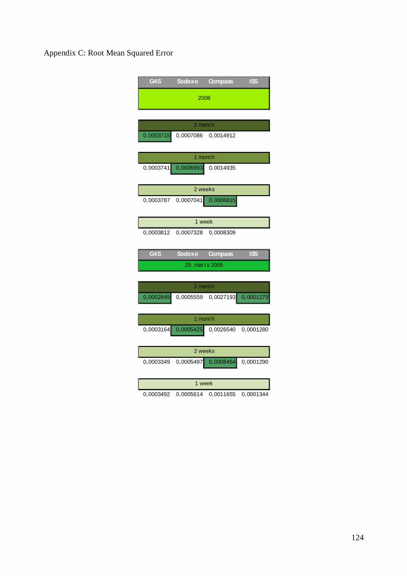
124

Appendix C: Root Mean Squared Error

G4S Sodexo Compass ISS

0,0003715 0,0007086 0,0014912

0,0003741 0,0006993 0,0014935

0,0003787 0,0007041 0,0006815

0,0003812 0,0007328 0,0008309

G4S Sodexo Compass ISS

0,0002849 0,0005559 0,0027193 0,0001279

0,0003164 0,0005425 0,0026540 0,0001280

0,0003349 0,0005497 0,0008454 0,0001290

0,0003492 0,0005614 0,0011655 0,0001344

2 month

1 month

2 weeks

1 week

2008

2 month

1 month

2 weeks

1 week

29. marts 2005

125

Appendix D: Binomial Distribution

Recovery Fraction (s) = 0,22 (f) = 0,78

u ssss sssf ssfs ssff sfss sfsf sffs sfff fsss fssf fsfs fsff ffss ffsf fffs ffffP(u) 0,002343 0,008305 0,008305 0,029447 0,008305 0,0294466 0,029447 0,104401 0,008305 0,029447 0,029447 0,104401 0,029447 0,104401 0,104401 0,370151

u 5*s 4*s 3*s 2*s 1*s 0*sP(u) 0,000515 0,001827 0,006478 0,022968 0,081433 0,2887174Occurence 1 5 10 10 5 1Acc prob 0,000515 0,009136 0,064782 0,229683 0,407166 0,2887174

5 trials

4 trials

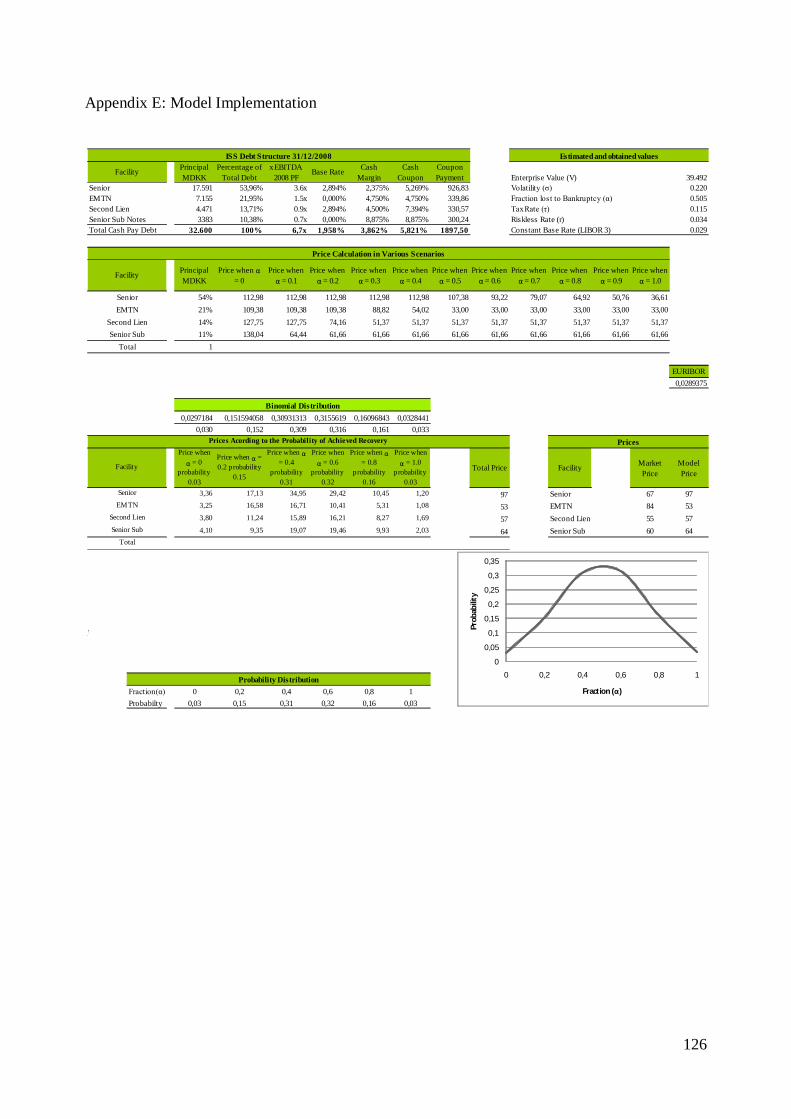
126

Appendix E: Model Implementation

Principal MDKK

Percentage of Total Debt

x EBITDA 2008 PF

Base Rate Cash Margin

Cash Coupon

Coupon Payment 39.492

17.591 53,96% 3.6x 2,894% 2,375% 5,269% 926,83 0.2207.155 21,95% 1.5x 0,000% 4,750% 4,750% 339,86 0.5054.471 13,71% 0.9x 2,894% 4,500% 7,394% 330,57 0.1153383 10,38% 0.7x 0,000% 8,875% 8,875% 300,24 0.034

32.600 100% 6,7x 1,958% 3,862% 5,821% 1897,50 0.029

Principal MDKK

Price when α = 0

Price when α = 0.1

Price when α = 0.2

Price when α = 0.3

Price when α = 0.4

Price when α = 0.5

Price when α = 0.6

Price when α = 0.7

Price when α = 0.8

Price when α = 0.9

Price when α = 1.0

54% 112,98 112,98 112,98 112,98 112,98 107,38 93,22 79,07 64,92 50,76 36,6121% 109,38 109,38 109,38 88,82 54,02 33,00 33,00 33,00 33,00 33,00 33,0014% 127,75 127,75 74,16 51,37 51,37 51,37 51,37 51,37 51,37 51,37 51,3711% 138,04 64,44 61,66 61,66 61,66 61,66 61,66 61,66 61,66 61,66 61,66

1

EURIBOR0,0289375

0,0297184 0,151594058 0,30931313 0,3155619 0,16096843 0,03284410,030 0,152 0,309 0,316 0,161 0,033

Price when α = 0

probability 0.03

Price when α = 0.2 probability

0.15

Price when α = 0.4

probability 0.31

Price when α = 0.6

probability 0.32

Price when α = 0.8

probability 0.16

Price when α = 1.0

probability 0.03

Total Price Facility Market Price

Model Price

3,36 17,13 34,95 29,42 10,45 1,20 97 Senior 67 973,25 16,58 16,71 10,41 5,31 1,08 53 EMTN 84 533,80 11,24 15,89 16,21 8,27 1,69 57 Second Lien 55 574,10 9,35 19,07 19,46 9,93 2,03 64 Senior Sub 60 64

Market price

Fraction(α) 0 0,2 0,4 0,6 0,8 1Probabilty 0,03 0,15 0,31 0,32 0,16 0,03

Total

Binomial Distribution

Facility

Senior

EMTNSecond Lien

Senior Sub

EMTNSecond LienSenior Sub

Total

Prices Acording to the Probability of Achieved Recovery Prices

Constant Base Rate (LIBOR 3)


Facility

SeniorEMTNSecond LienSenior Sub NotesTotal Cash Pay Debt

Probability Distribution


Facility

Senior

Riskless Rate (r)

Estimated and obtained values

Enterprise Value (V)Volatility (σ)Fraction lost to Bankruptcy (α)Tax Rate (τ)

0

0,05

0,1

0,15

0,2

0,25

0,3

0,35

0 0,2 0,4 0,6 0,8 1

Prob

abili

ty

Fraction (α)

127

Appendix F: Stress Tests

Principal MDKK

Percentage of Total

x EBITDA 2008 PF


Cash Coupon

Coupon Payment17.591 53,96% 3.6x 2,894% 2,375% 5,269% 926,83 EURIBOR

7.155 21,95% 1.5x 0,000% 4,750% 4,750% 339,86 0,02893754.471 13,71% 0.9x 2,894% 4,500% 7,394% 330,573383 10,38% 0.7x 0,000% 8,875% 8,875% 300,24

Total Cash Pay Debt 32.600 100% 6,7x 1,958% 3,862% 5,821% 1897,50

Principal MDKK

Price when α = 0

Price when α = 0.1

Price when α = 0.2

Price when α = 0.3

Price when α = 0.4

Price when α = 0.5

Price when α = 0.6

Price when α = 0.7

Price when α = 0.8

Price when α =

0.9

Price when α = 1.0

17.591 112,98 112,98 112,98 112,98 112,98 112,98 112,98 112,98 112,98 112,98 112,987.155 109,38 109,38 109,38 109,38 109,38 109,38 109,38 109,38 109,38 109,38 109,384.471 127,75 127,75 127,75 127,75 127,75 127,75 127,75 127,75 127,75 127,75 127,753.383 138,04 138,04 138,04 138,04 138,04 138,04 138,04 138,04 138,04 138,04 138,04

32.6000,00 0,01 0,06 0,23 0,41 0,29

Principal M DKK

Price when α = 0

Price when α = 0.2

Price when α = 0.4

Price when α = 0.6

Price when α = 0.8

Price when α = 1.0

Total Price

Enterprise Value (V) 39.49217.591 0,06 1,03 7,32 25,95 46,00 32,62 113 Volatility (σ) 0.227.155 0,06 1,00 7,09 25,12 44,54 31,58 109 Fraction lost to Bankruptcy (α) 0.34.471 0,07 1,17 8,28 29,34 52,01 36,88 128 Tax Rate (τ) 0.1153.383 0,07 1,26 8,94 31,71 56,21 39,85 138 Riskless Rate (r) 0.034

32.600 Constant Base Rate (LIBOR 3) 0,02894

-10% -5% 0% 5% 10% -10% -5% 0% 5% 10%100 98 97 95 94 Senior 100 98 97 94 9259 56 53 51 49 EMTN 59 56 53 51 4867 62 57 53 49 Second Lien 60 58 57 56 5576 70 64 59 54 Senior Sub 65 65 64 63 63

-10% -5% 0% 5% 10% Facility Market Price

Model Price

87 92 97 100 104 Senior 67 11340 47 53 59 64 EMTN 84 10932 45 57 68 77 Second Lien 55 12832 49 64 77 89 Senior Sub 60 138

S

Volatility EV Alpha Volatility EV Alpha Volatility EV Alpha Volatility EV Alpha Volatility EV AlphaSenior # 87 100 98 92 98 97 97 97 95 100 94 94 104 92EMTN # 40 59 56 47 56 53 53 53 51 59 51 49 64 48Second Lien # 32 60 62 45 58 57 57 57 53 68 56 49 77 55Senior Sub # 32 65 70 49 65 64 64 64 59 77 63 54 89 63

Senior EMTN

Second LienSenior Sub

Fraction lost to Bankruptcy costs Stress Test

Enterprise Value Stress Test Prices

Facility

Senior EMTN


Facility


Volatility Stress Test


FacilitySenior

EMTN


Total

Senior

Facility

EMTN


ISS Debt Structure 31/12/2008Facility

-10% -5% 0% 5% 10%Facility


Total

Facility


SeniorEMTN

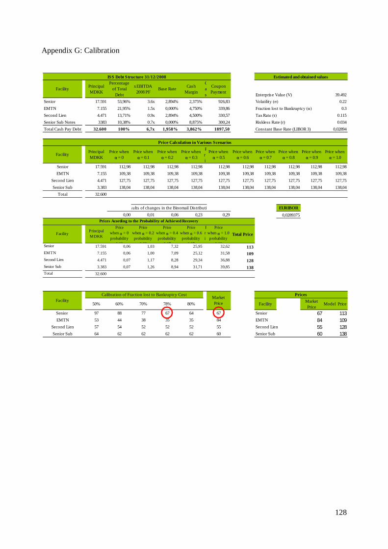
128

Appendix G: Calibration

Principal MDKK

Percentage of Total

Debt

x EBITDA 2008 PF


Cas

Coupon Payment Enterprise Value (V) 39.492

17.591 53,96% 3.6x 2,894% 2,375% 926,83 Volatility (σ) 0.227.155 21,95% 1.5x 0,000% 4,750% 339,86 Fraction lost to Bankruptcy (α) 0.34.471 13,71% 0.9x 2,894% 4,500% 330,57 Tax Rate (τ) 0.1153383 10,38% 0.7x 0,000% 8,875% 300,24 Riskless Rate (r) 0.034

32.600 100% 6,7x 1,958% 3,862% 1897,50 Constant Base Rate (LIBOR 3) 0,02894

Principal MDKK

Price when α = 0

Price when α = 0.1

Price when α = 0.2

Price when α = 0.3

Pri

Price when α = 0.5

Price when α = 0.6

Price when α = 0.7

Price when α = 0.8

Price when α = 0.9

Price when α = 1.0

17.591 112,98 112,98 112,98 112,98 112,98 112,98 112,98 112,98 112,98 112,987.155 109,38 109,38 109,38 109,38 109,38 109,38 109,38 109,38 109,38 109,384.471 127,75 127,75 127,75 127,75 127,75 127,75 127,75 127,75 127,75 127,753.383 138,04 138,04 138,04 138,04 138,04 138,04 138,04 138,04 138,04 138,04

32.600

EURIBOR0,00 0,01 0,06 0,23 0,29 0,0289375

Principal MDKK

Price when α = 0 probability

0.02


0.03


0.07


0.25

Pric


0.02

Total Price

17.591 0,06 1,03 7,32 25,95 32,62 1137.155 0,06 1,00 7,09 25,12 31,58 1094.471 0,07 1,17 8,28 29,34 36,88 1283.383 0,07 1,26 8,94 31,71 39,85 138

32.600

50% 60% 70% 78% 80% Facility Market Price

Model Price

97 88 77 67 64 67 Senior 67 11353 44 38 35 35 84 EMTN 84 10957 54 52 52 52 55 Second Lien 55 12864 62 62 62 62 60 Senior Sub 60 138

Senior EMTN



EMTN


Facility

SeniorEMTNSecond LienSenior Sub NotesTotal Cash Pay Debt


Facility

Senior

EMTN

Second Lien

Senior Sub


Total


Facility

Senior

Results of changes in the Binomail Distribution

Prices

Total

Calibration of Fraction lost to Bankruptcy Cost Market PriceFacility

Documents

A theoretical approach to pricing leveraged loans - StudentTheses