AASHTO Design Equation

(Rigid Pavements)

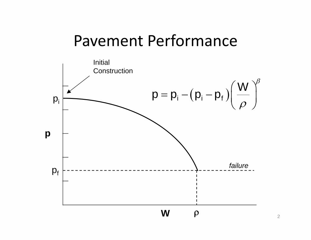
Pavement Performance

2

p

W

i i fWp p p p

failure

pi

pf

InitialConstruction

Pavement Performance

3

p

W

Wp 1.4.5 4.5 5

failure

4.5

1.5

InitialConstruction

Pavement Performance

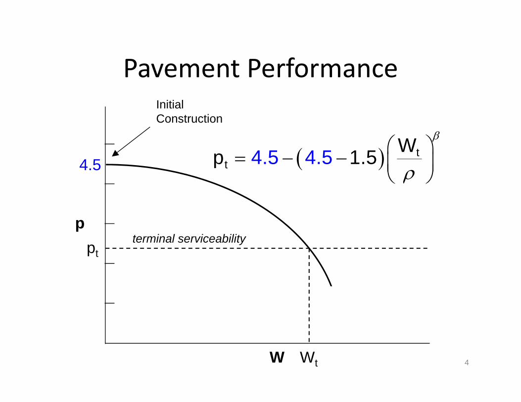
4

p

t

tWp 1.54.5 4.54.5

pt

InitialConstruction

terminal serviceability

WtW

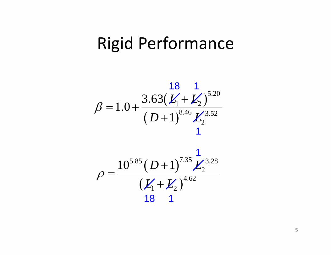
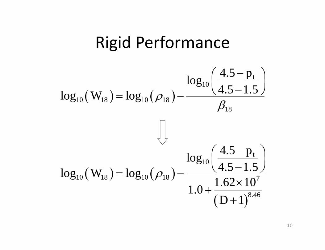
Rigid Performance

5

7.355.85 3.282

4.621 2

10 1

D L

L L

5.201 2

8.46 3.522

3.631.01

L LD L

18

18

1

1

1

1

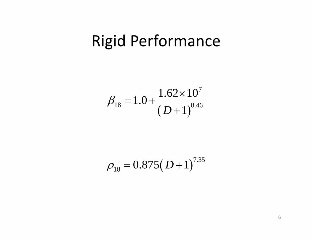
Rigid Performance

6

7.3518 0.875 1 D

7

18 8.461.62 101.0

1

D

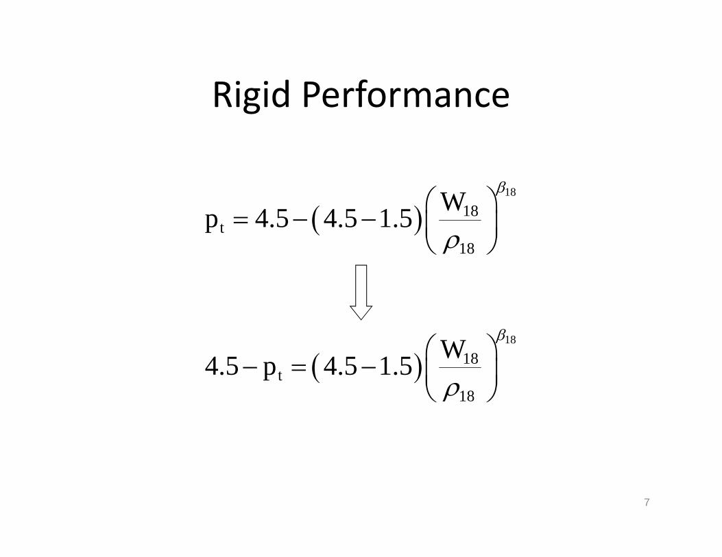
Rigid Performance

7

18

18t

18

Wp 4.5 4.5 1.5

18

18t

18

W4.5 p 4.5 1.5

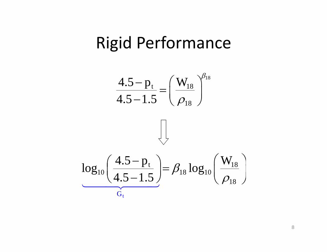
Rigid Performance

8

18

t 18

18

4.5 p W4.5 1.5

tG

t 1810 18 10

18

4.5 p Wlog log4.5 1.5

Rigid Performance

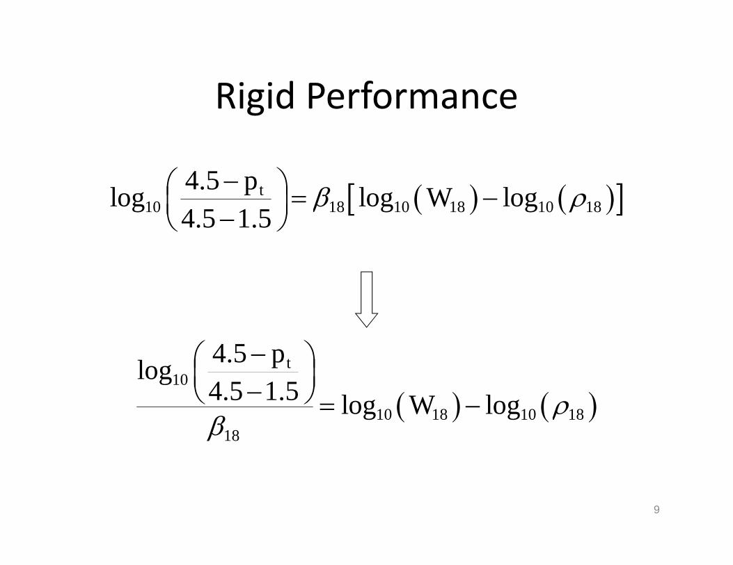
9

t10 18 10 18 10 18

4.5 plog log W log4.5 1.5

t

10

10 18 10 1818

4.5 plog4.5 1.5 log W log

Rigid Performance

10

t

10

10 18 10 1818

4.5 plog4.5 1.5log W log

t10

10 18 10 18 7

8.46

4.5 plog4.5 1.5log W log

1.62 101.0D 1

Rigid Performance

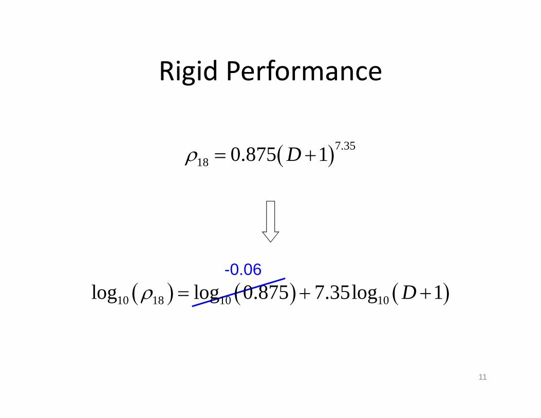
11

-0.06 10 18 10 10log log 0.875 7.35log 1 D

7.3518 0.875 1 D

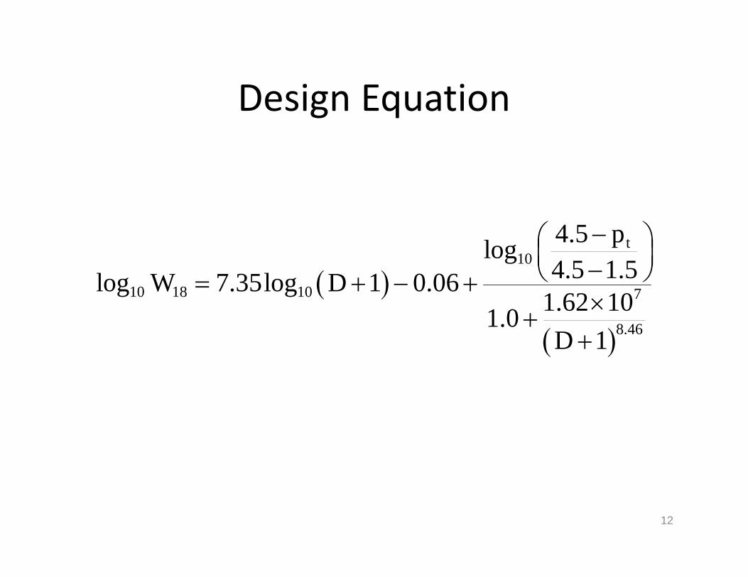
Design Equation

12

t10

10 18 10 7

8.46

4.5 plog4.5 1.5log W 7.35log D 1 0.06

1.62 101.0D 1

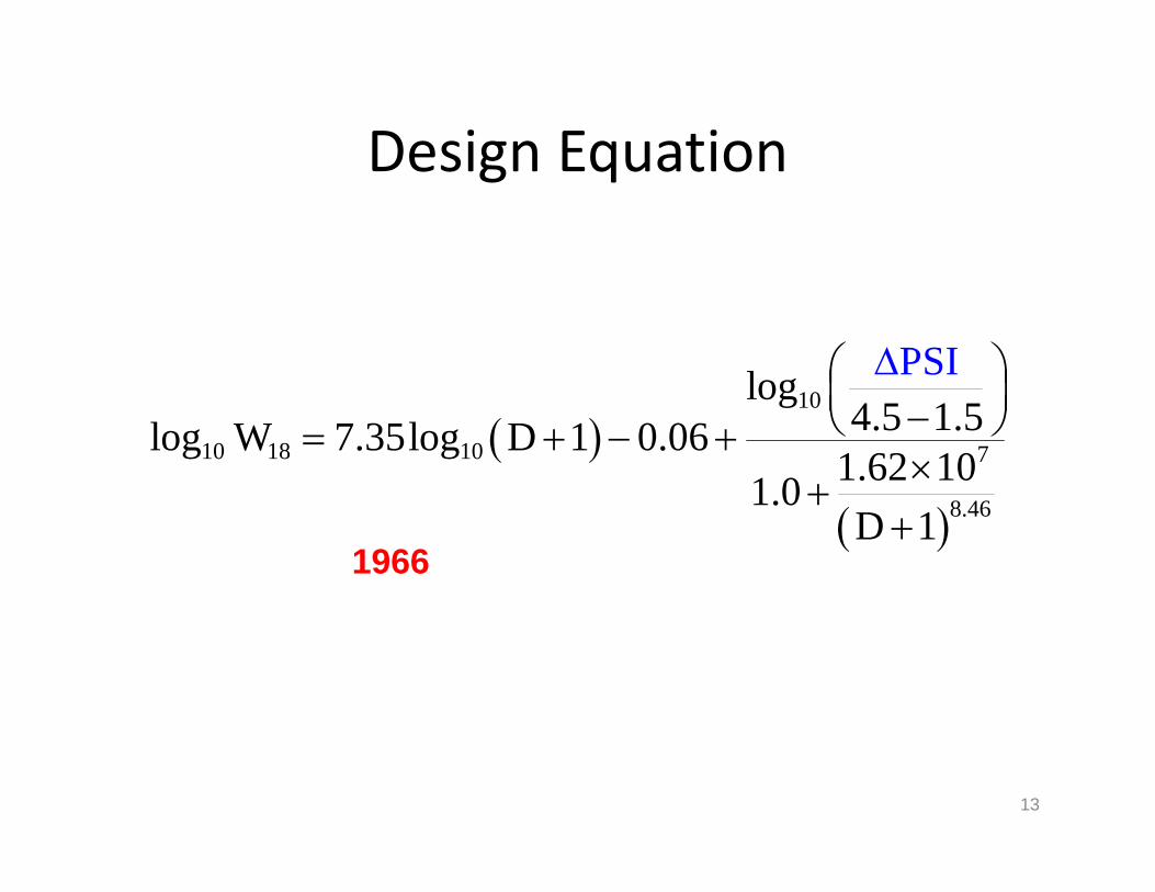
Design Equation

13

1966

10

10 18 10 7

8.46

PSlog4.5 1.5log W 7.35log D 1 0.06

1.62 101.0D

I

1

Design Equation

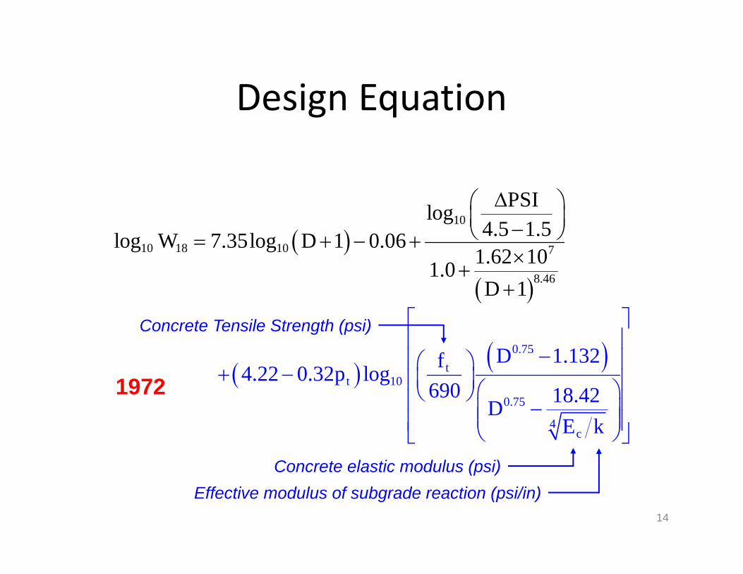
14

10

10 18 10 7

8.46

PSIlog4.5 1.5log W 7.35log D 1 0.06

1.62 101.0D 1

0.75t

t 10

0.75

4c

D 1.132f4.22 0.32p log690 18.42D

E k

1972

Concrete Tensile Strength (psi)

Concrete elastic modulus (psi)Effective modulus of subgrade reaction (psi/in)

Design Equation

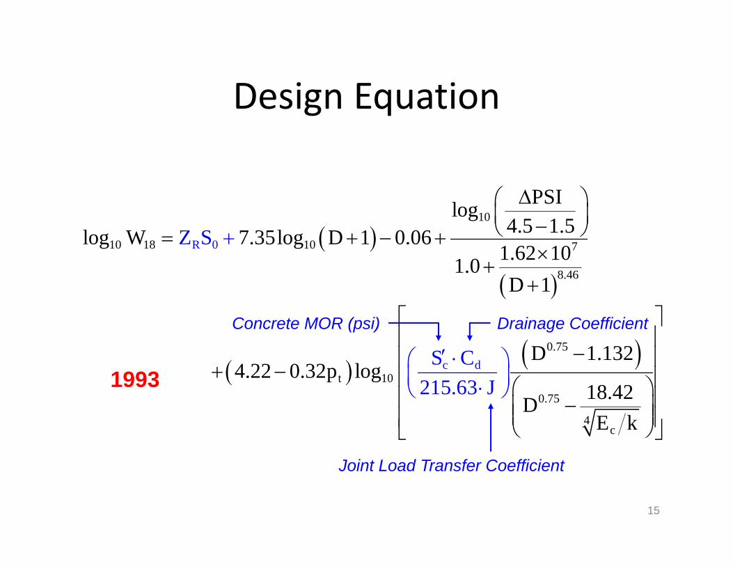
15

10

10 18 10 7

.

R

8

0

46

PSIlog4.5 1.5log W 7.35log D 1 0.06

1.62 101

Z S1.0

D

0.75

t 10

0.75

4c

c dS C215.6

D 1.1324.22 0.3

3 J2p log

18.42DE k

1993

Concrete MOR (psi) Drainage Coefficient

Joint Load Transfer Coefficient

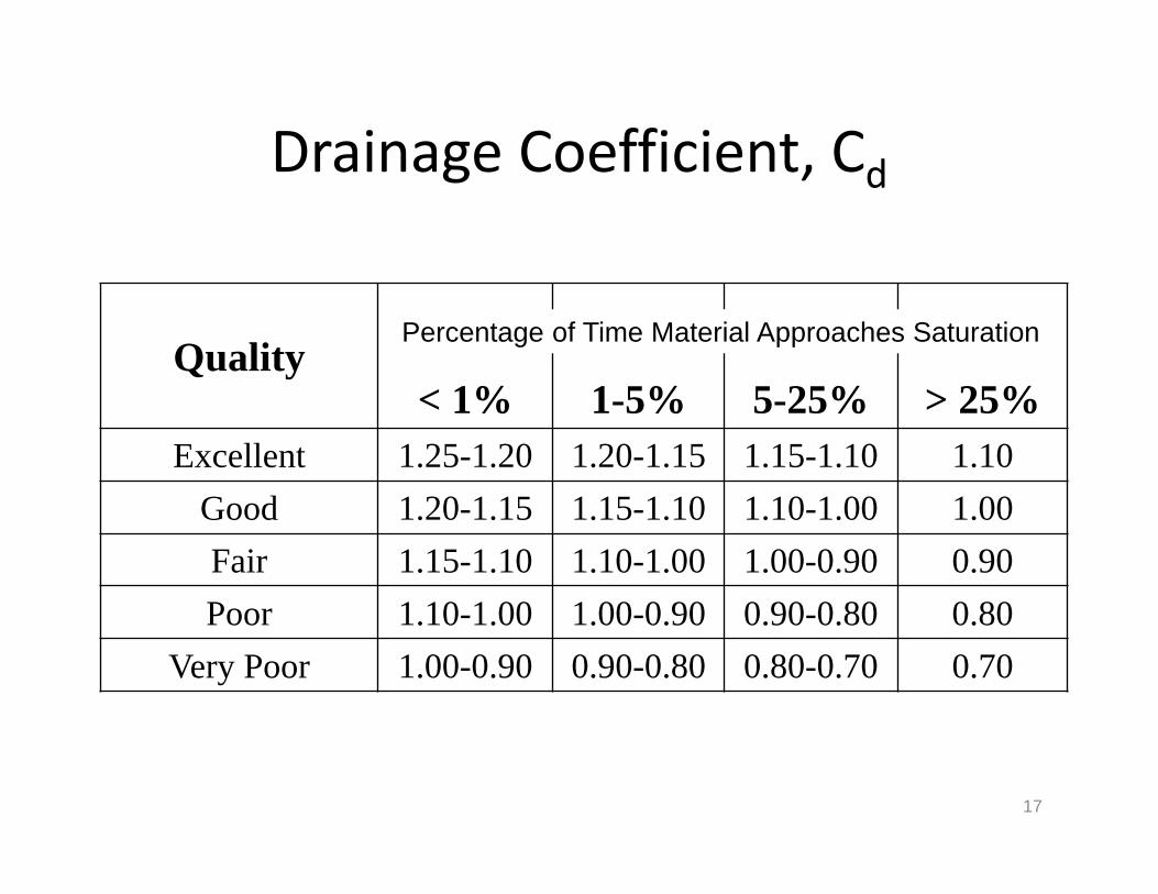
Drainage Coefficient, Cd

17

Quality< 1% 1-5% 5-25% > 25%

Excellent 1.25-1.20 1.20-1.15 1.15-1.10 1.10Good 1.20-1.15 1.15-1.10 1.10-1.00 1.00Fair 1.15-1.10 1.10-1.00 1.00-0.90 0.90Poor 1.10-1.00 1.00-0.90 0.90-0.80 0.80

Very Poor 1.00-0.90 0.90-0.80 0.80-0.70 0.70

Percentage of Time Material Approaches Saturation

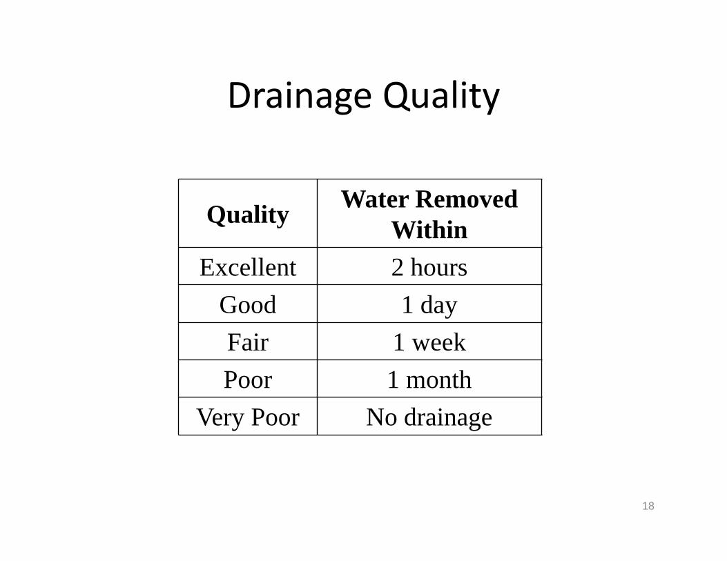
Drainage Quality

18

Quality Water Removed Within

Excellent 2 hoursGood 1 dayFair 1 weekPoor 1 month

Very Poor No drainage

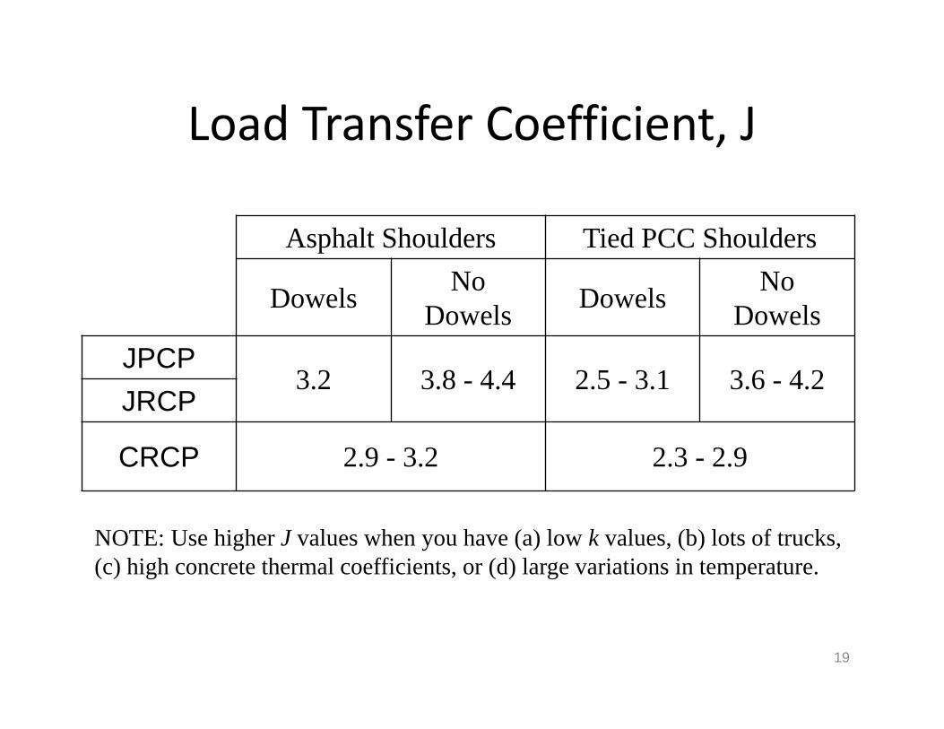
Load Transfer Coefficient, J

19

Asphalt Shoulders Tied PCC Shoulders

Dowels NoDowels Dowels No

DowelsJPCP

3.2 3.8 - 4.4 2.5 - 3.1 3.6 - 4.2JRCP

CRCP 2.9 - 3.2 2.3 - 2.9

NOTE: Use higher J values when you have (a) low k values, (b) lots of trucks, (c) high concrete thermal coefficients, or (d) large variations in temperature.

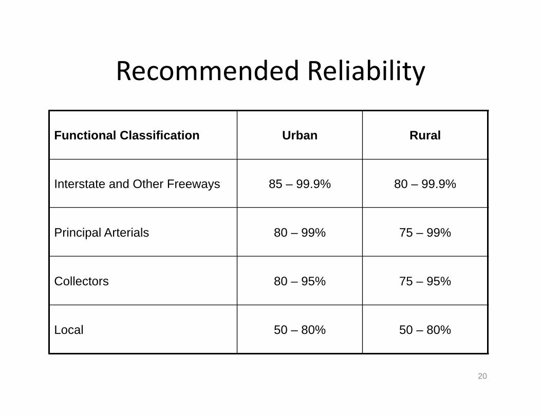
Recommended Reliability

Functional Classification Urban Rural

Interstate and Other Freeways 85 – 99.9% 80 – 99.9%

Principal Arterials 80 – 99% 75 – 99%

Collectors 80 – 95% 75 – 95%

Local 50 – 80% 50 – 80%

20

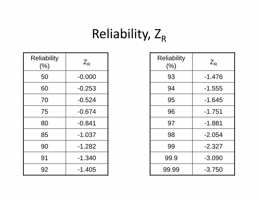
Reliability, ZRReliability

(%) ZRReliability

(%) ZR

50 -0.000 93 -1.476

60 -0.253 94 -1.555

70 -0.524 95 -1.645

75 -0.674 96 -1.751

80 -0.841 97 -1.881

85 -1.037 98 -2.054

90 -1.282 99 -2.327

91 -1.340 99.9 -3.090

92 -1.405 99.99 -3.750

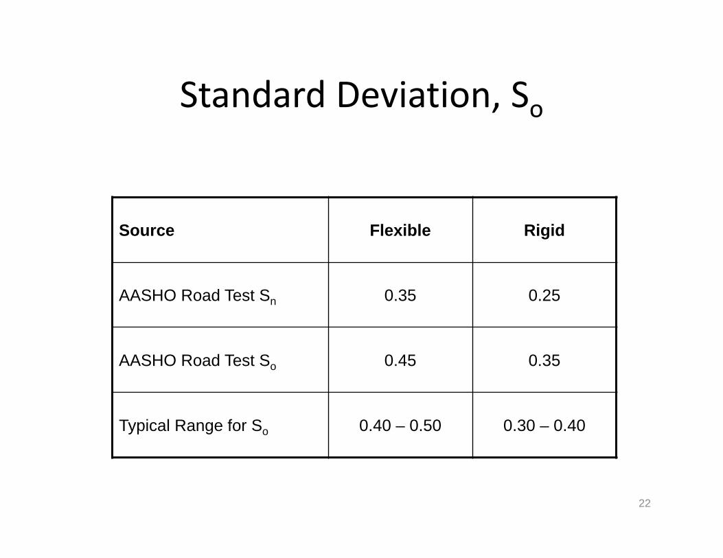
Standard Deviation, So

Source Flexible Rigid

AASHO Road Test Sn 0.35 0.25

AASHO Road Test So 0.45 0.35

Typical Range for So 0.40 – 0.50 0.30 – 0.40

22

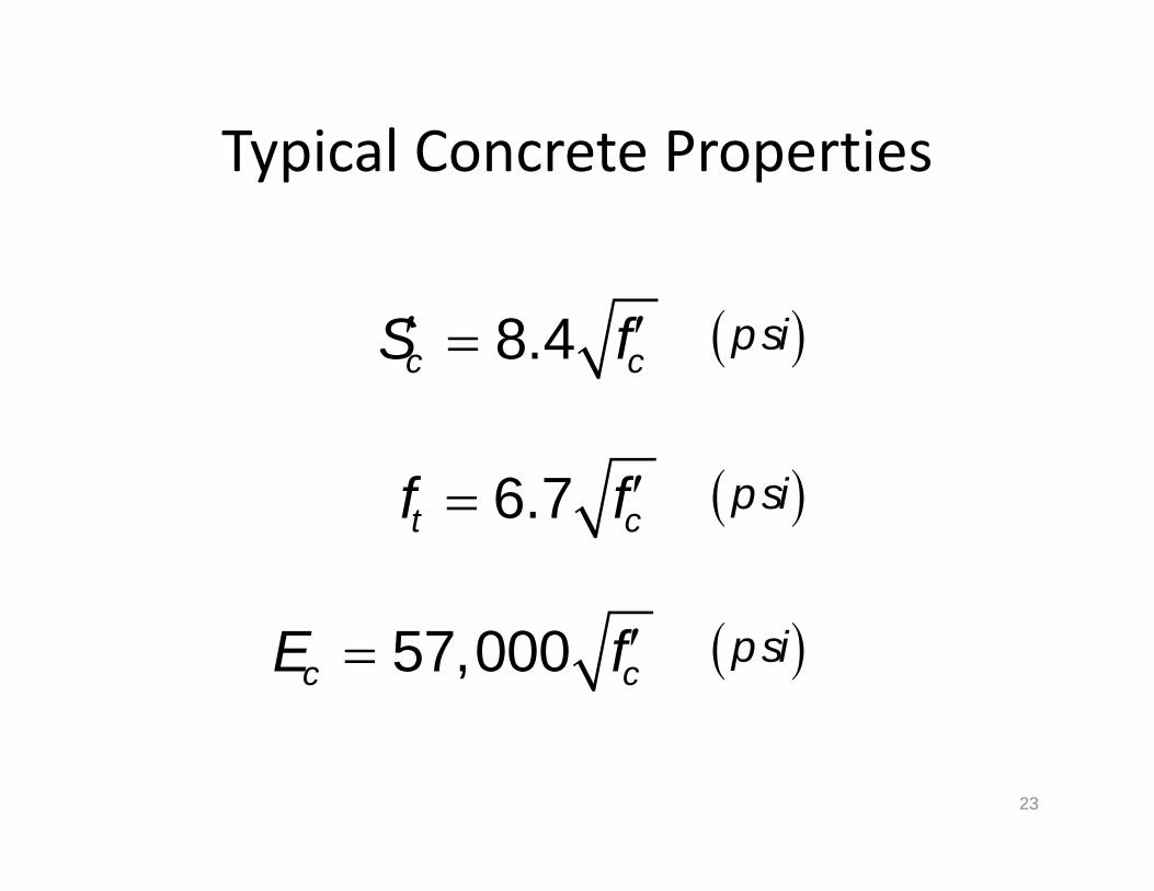
Typical Concrete Properties

23

8.4c cS f psi

6.7t cf f psi

57,000c cE f psi

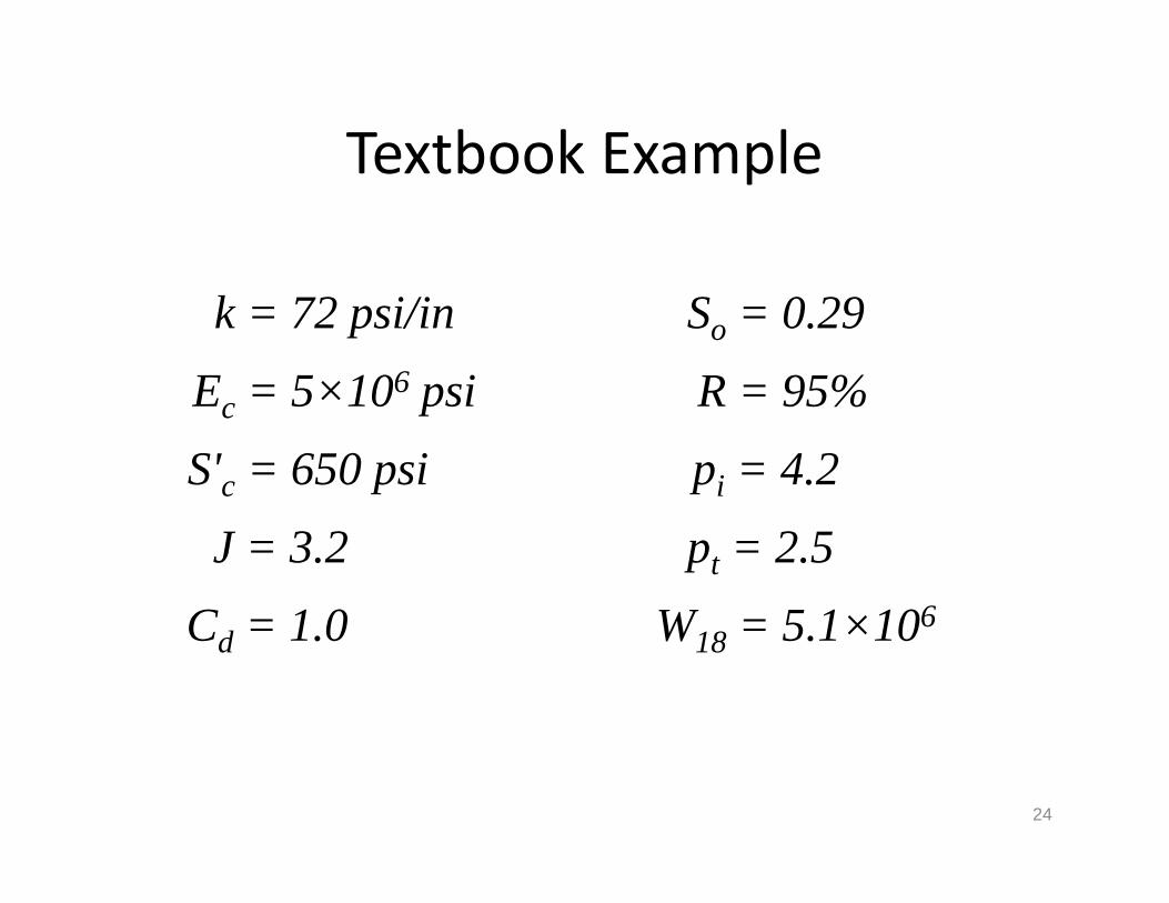
Textbook Example

24

J = 3.2

So = 0.29k = 72 psi/in

Ec = 5×106 psi

S'c = 650 psi

Cd = 1.0

R = 95%

pi = 4.2

W18 = 5.1×106

pt = 2.5

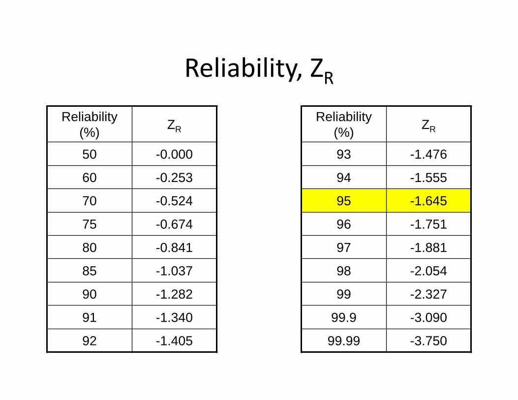
Reliability, ZRReliability

(%) ZRReliability

(%) ZR

50 -0.000 93 -1.476

60 -0.253 94 -1.555

70 -0.524 95 -1.645

75 -0.674 96 -1.751

80 -0.841 97 -1.881

85 -1.037 98 -2.054

90 -1.282 99 -2.327

91 -1.340 99.9 -3.090

92 -1.405 99.99 -3.750

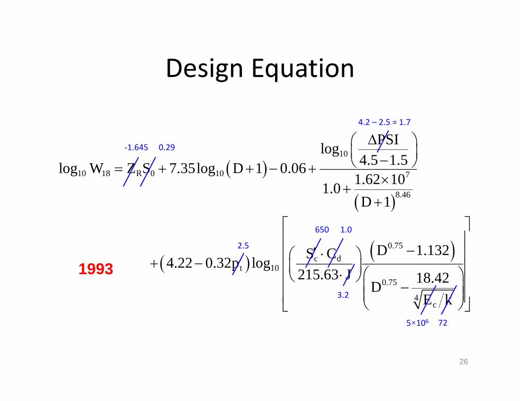
Design Equation

26

10

10 18 R 0 10 7

8.46

PSIlog4.5 1.5log W Z S 7.35log D 1 0.06

1.62 101.0D 1

0.75c d

t 10

0.75

4c

D 1.132S C4.22 0.32p log215.63 J 18.42D

E k

1993

‐1.645 0.29

4.2 – 2.5 = 1.7

2.5

650 1.0

3.2

5×106 72

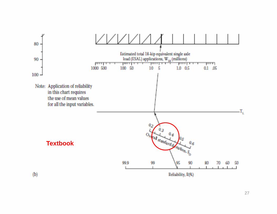
27

Textbook

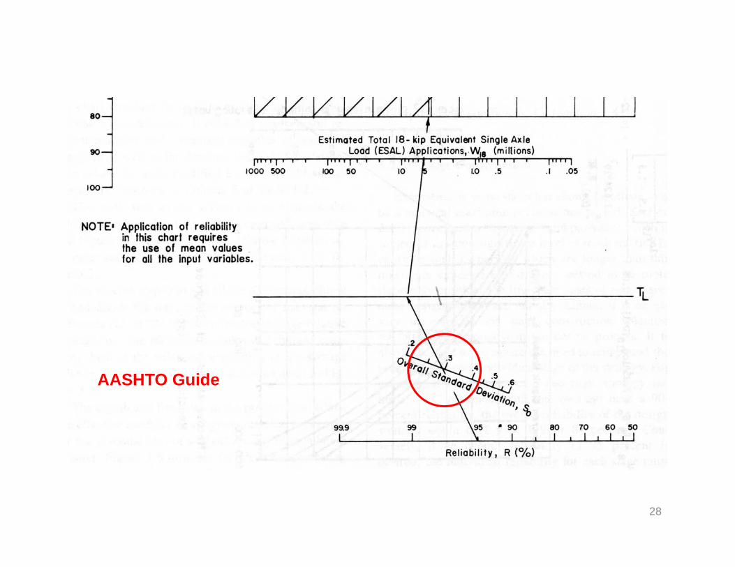
28

AASHTO Guide

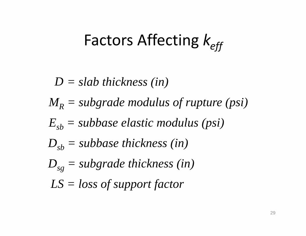
Factors Affecting keff

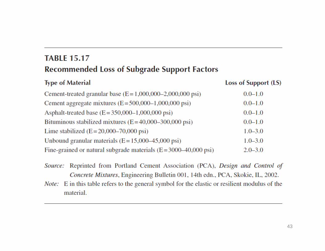
29

Dsb = subbase thickness (in)

LS = loss of support factor

= slab thickness (in)D

MR = subgrade modulus of rupture (psi)

Esb = subbase elastic modulus (psi)

Dsg = subgrade thickness (in)

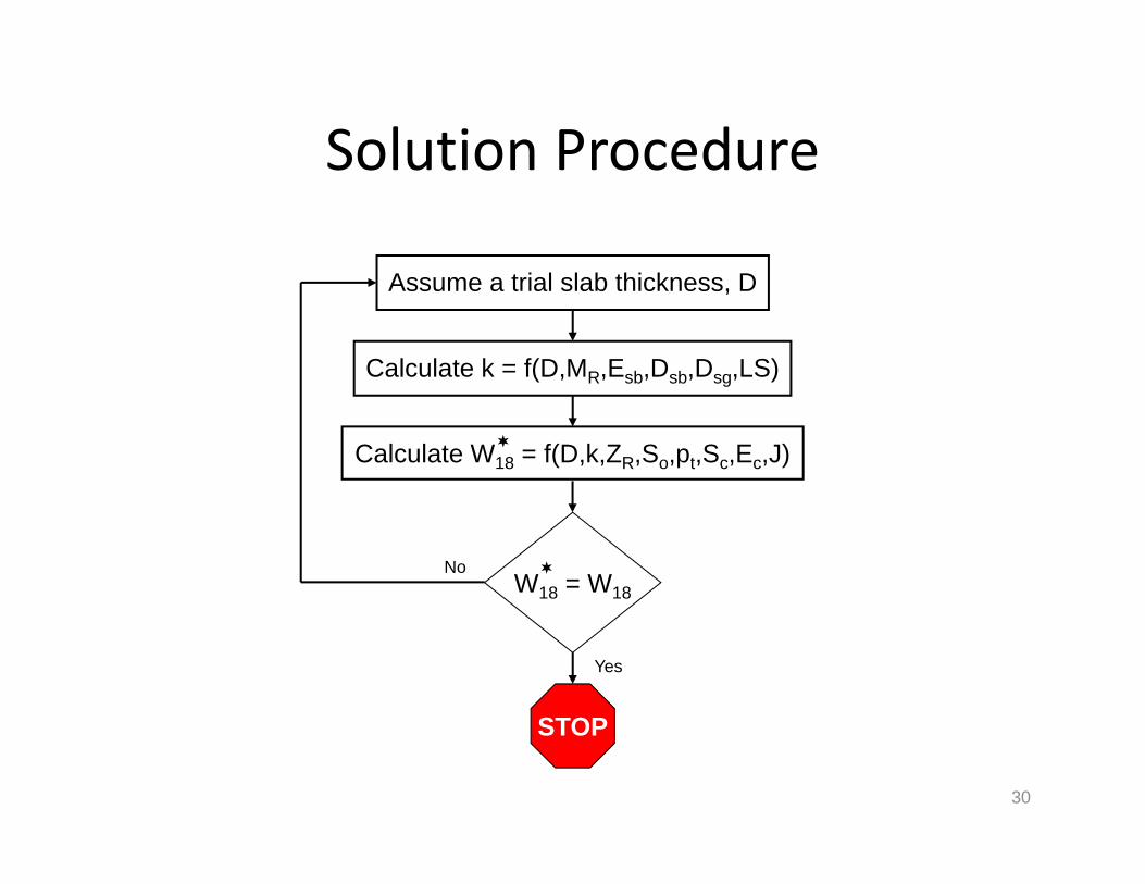
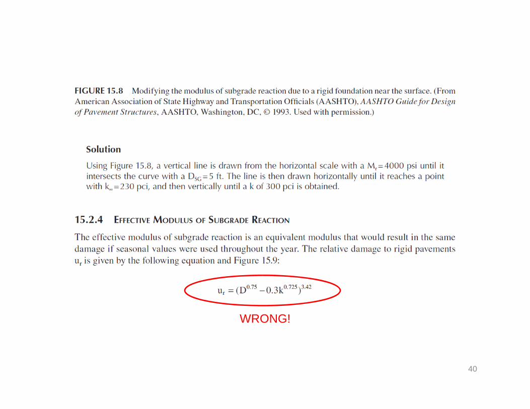
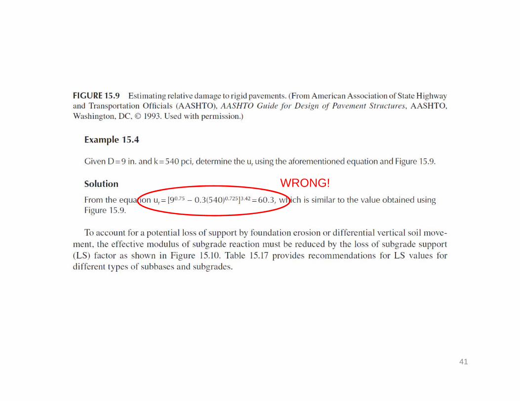
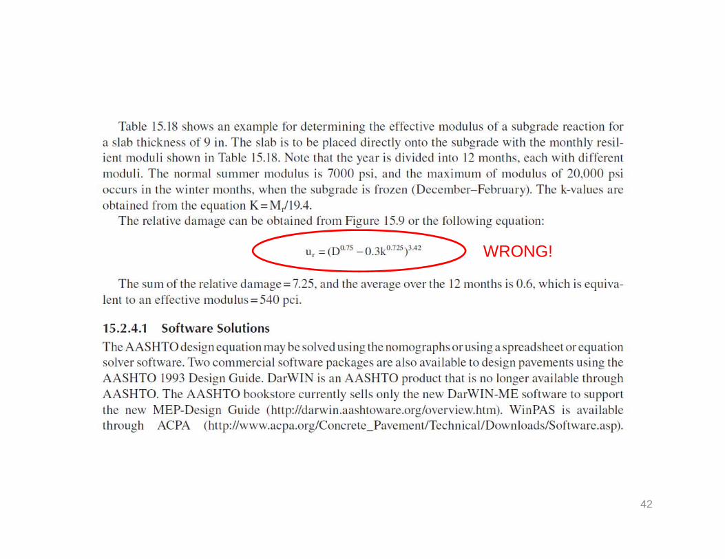
Solution Procedure

30

Assume a trial slab thickness, D

Calculate k = f(D,MR,Esb,Dsb,Dsg,LS)

Calculate W18 = f(D,k,ZR,So,pt,Sc,Ec,J)

W18 = W18

STOP

Yes

No

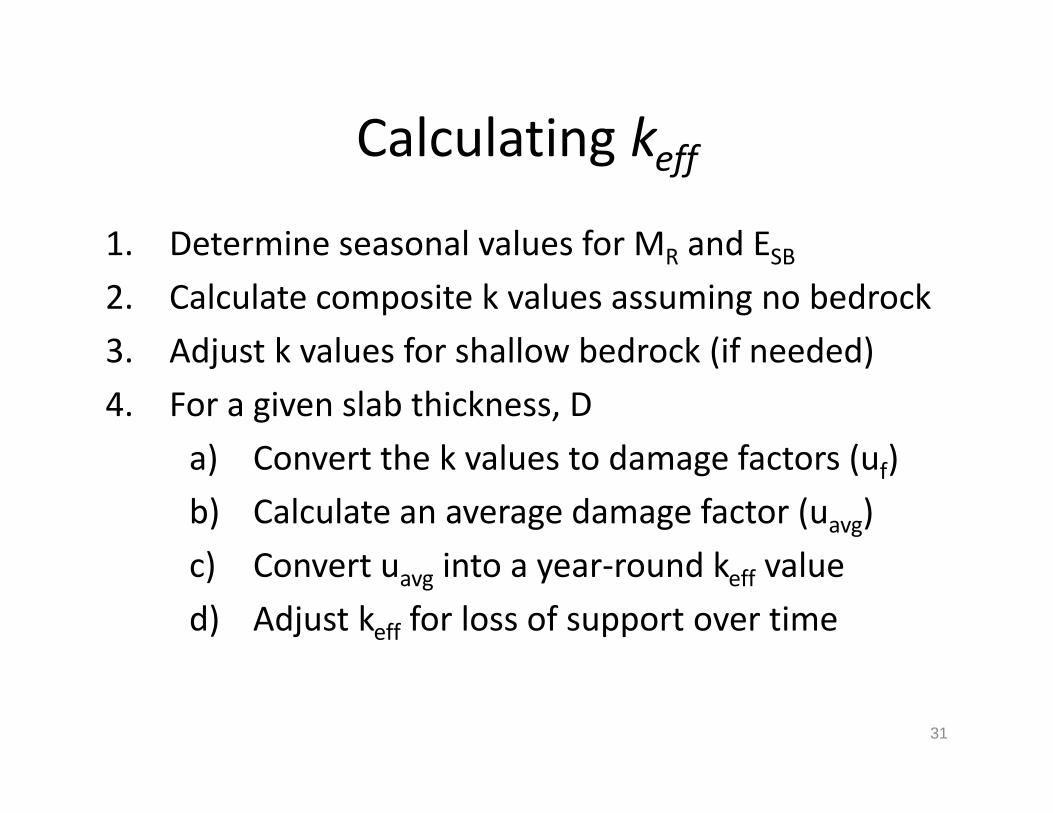
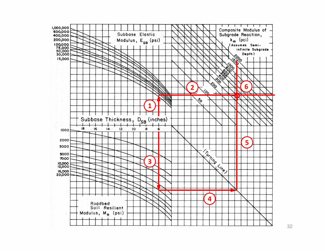
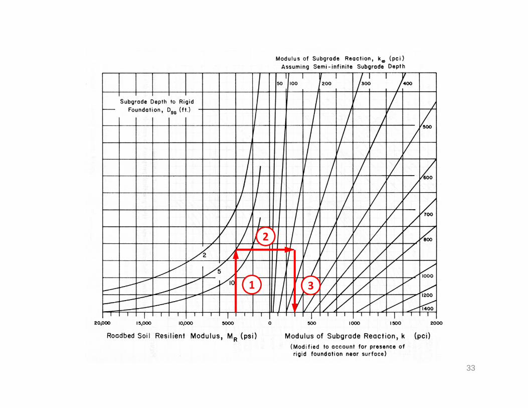
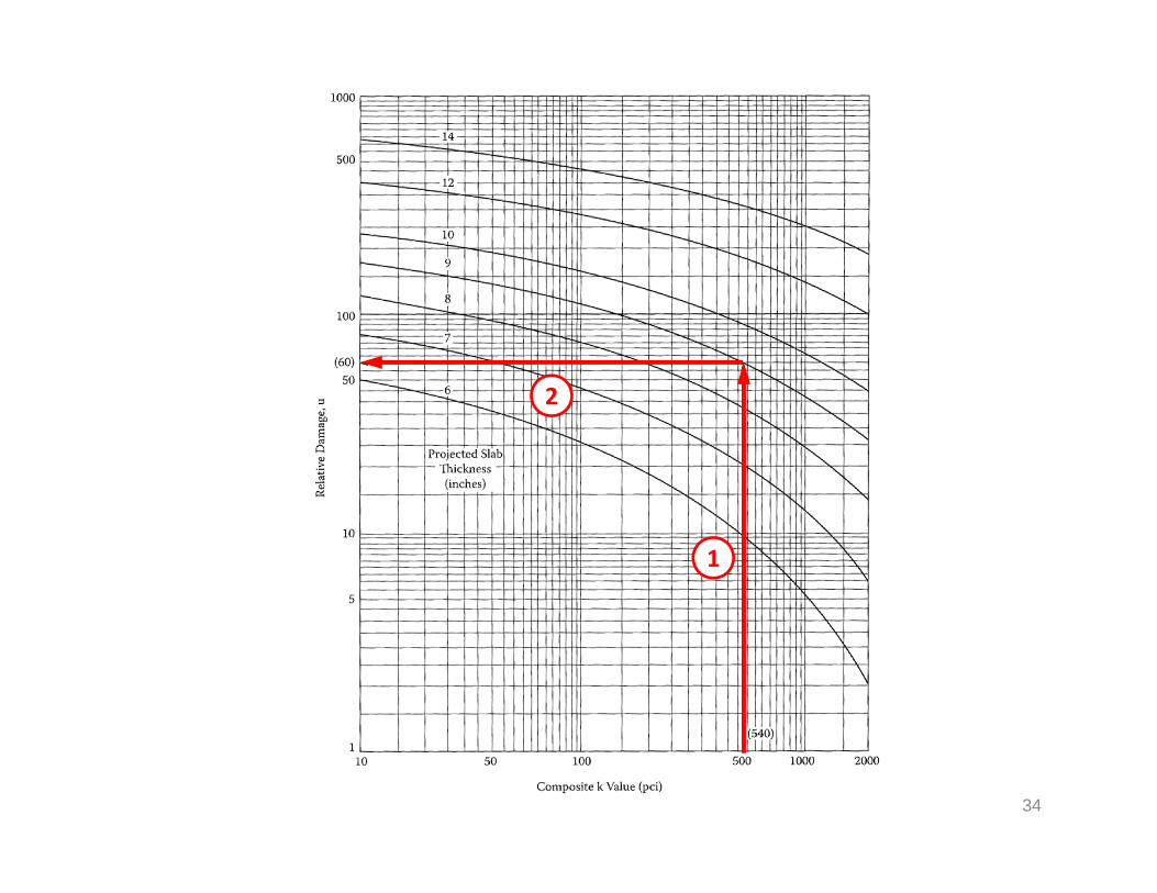
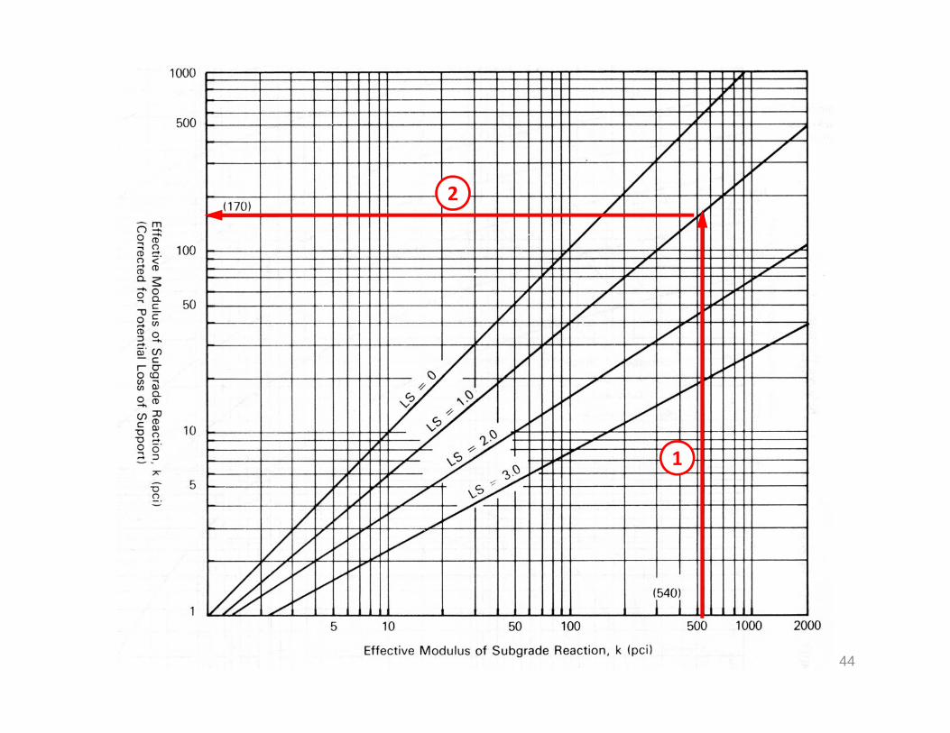
Calculating keff

31

1. Determine seasonal values for MR and ESB2. Calculate composite k values assuming no bedrock3. Adjust k values for shallow bedrock (if needed)4. For a given slab thickness, D

a) Convert the k values to damage factors (uf)b) Calculate an average damage factor (uavg)c) Convert uavg into a year‐round keff valued) Adjust keff for loss of support over time

1

2

3

4

5

6

32

1

2

3

33

34

1

2

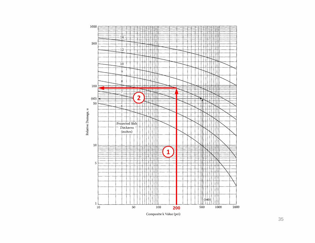
35

1

2

200

2

1

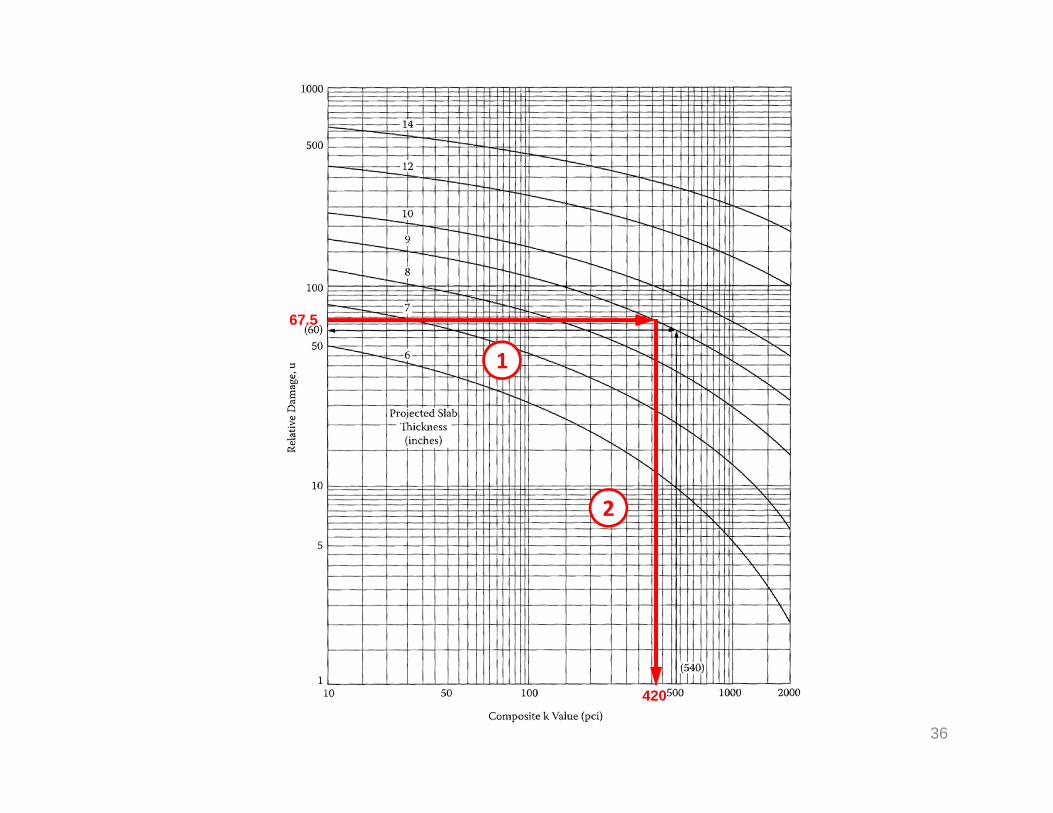
36

420

67.5

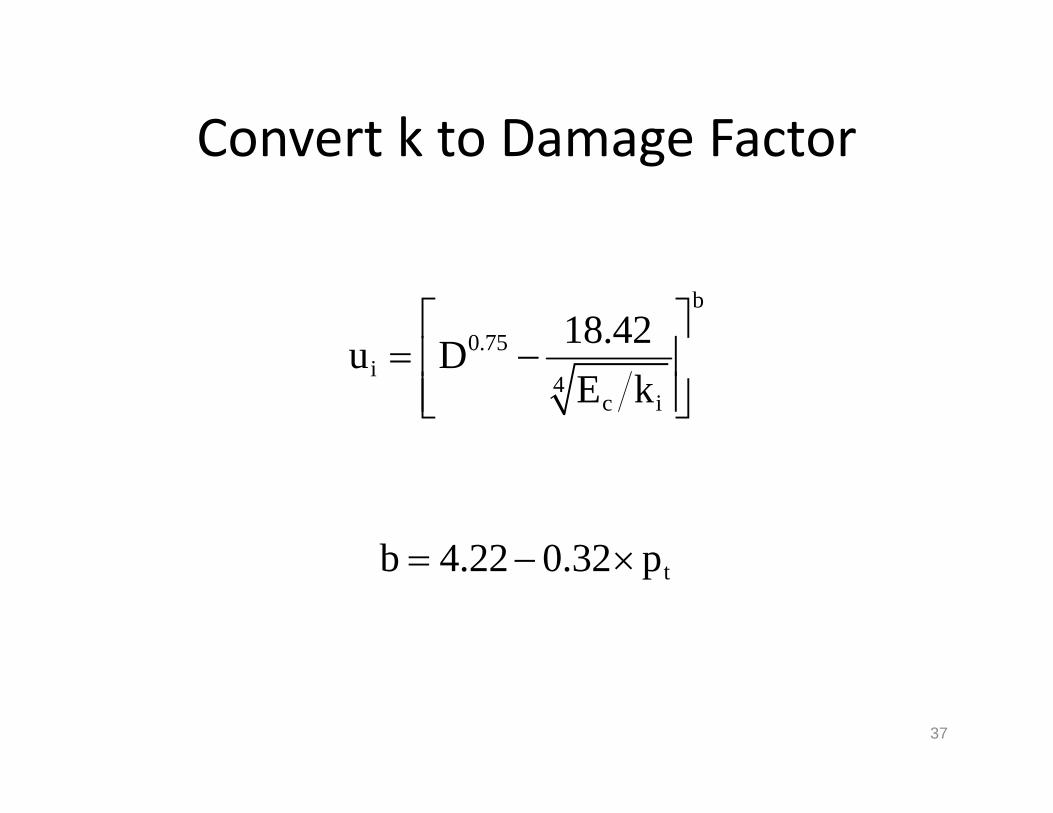
Convert k to Damage Factor

37

b

0.75i

4c i

18.42u DE k

tb 4.22 0.32 p

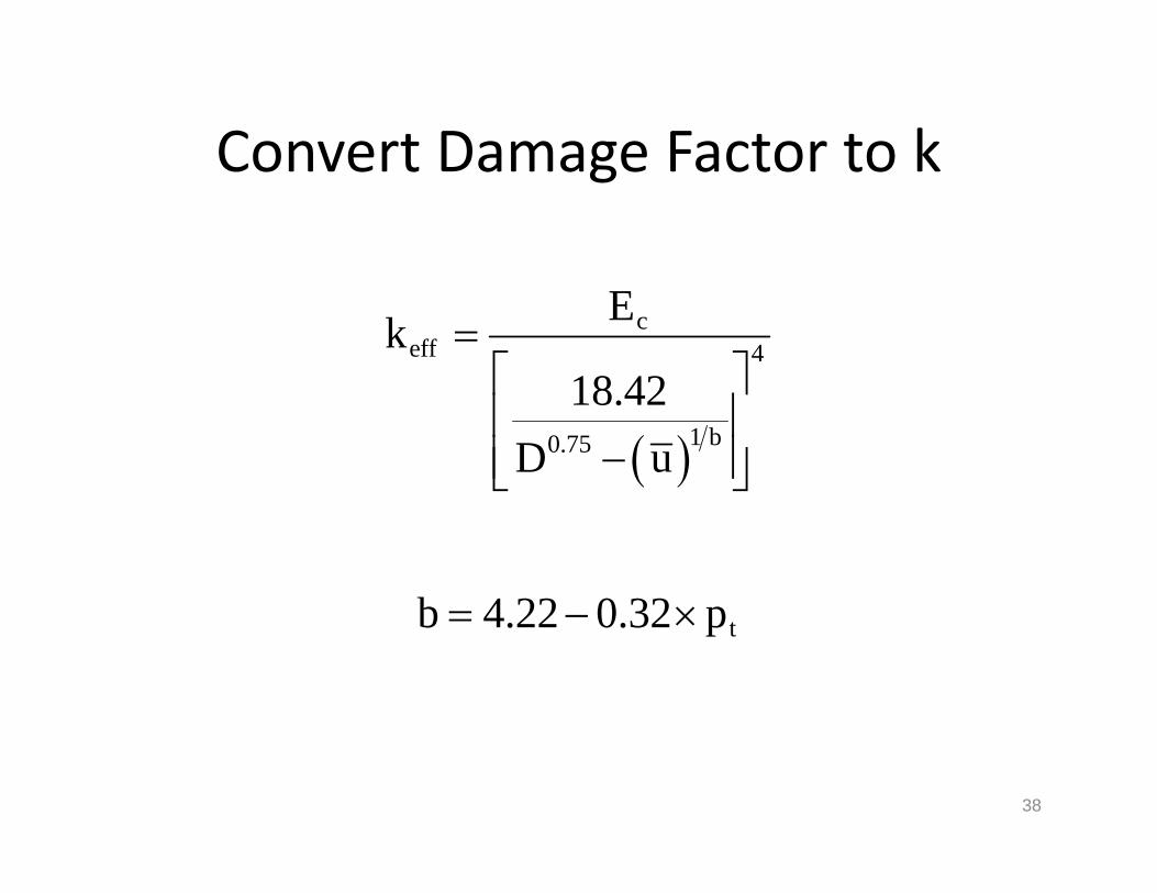
Convert Damage Factor to k

38

ceff 4

1 b0.75

Ek18.42

D u

tb 4.22 0.32 p

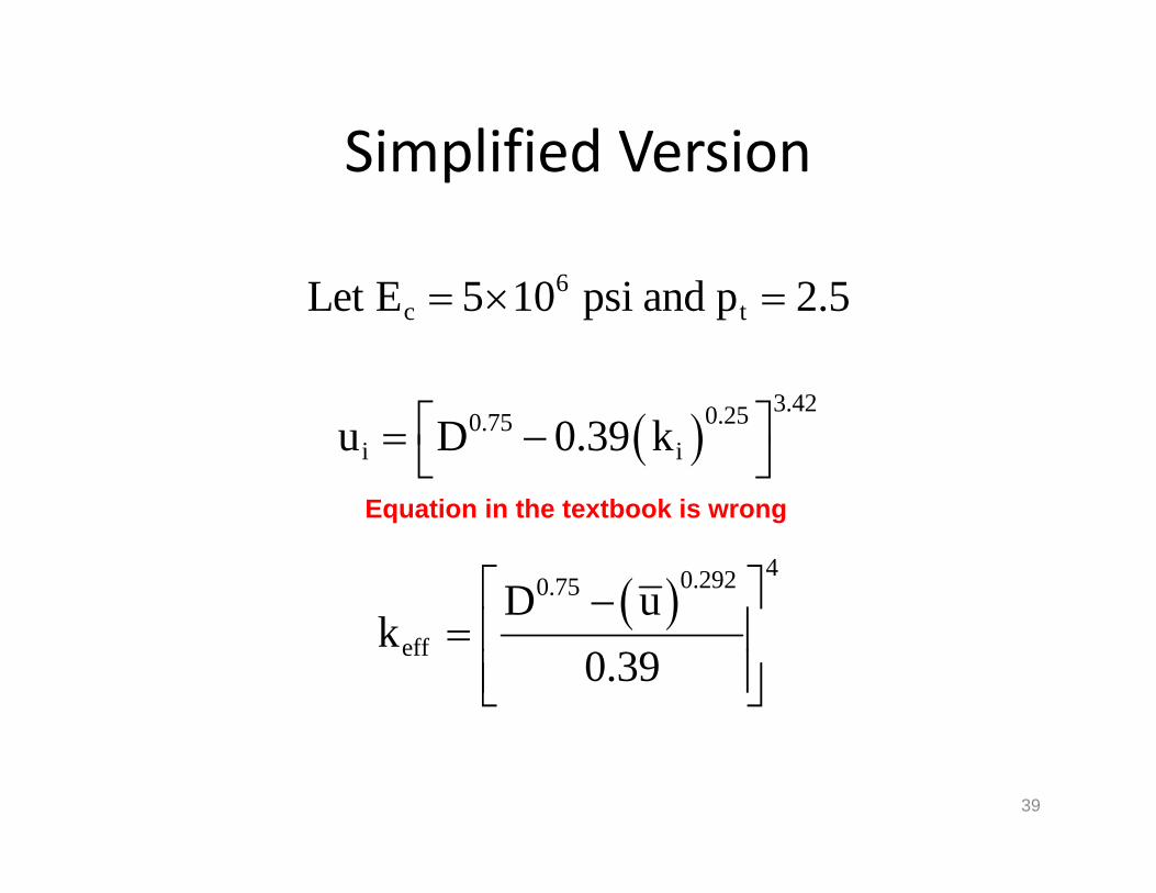
Simplified Version

39

3.420.250.75

i iu D 0.39 k

6c tLet E 5 10 psi and p 2.5

40.2920.75

effD u

k0.39

Equation in the textbook is wrong

40

WRONG!

41

WRONG!

42

WRONG!

43

1

2

44