1 of 15

Acoustic Velocity Determination for AUT on Spiral Pipe Girth Welds

Ed GINZEL 1

Henk VAN DIJK 2 1 Materials Research Institute, Waterloo, Ontario, Canada e-mail: eginzel@mri.on.ca

2 JES Pipelines, Willemstad, Curacao email henk.jes@autservices.com

2015.09.27

Abstract Determining acoustic velocity is a critical aspect for the correct calculation of Snell’s Law to determine refracted angle and to position the location of flaws along the soundpath of an ultrasonic beam. This has been seen as a critical part of preparations in girth weld inspections using zonal discrimination where it is mandated by codes. The typical steels used in pipeline construction are slightly anisotropic, making it necessary to determine the shear velocities at different angles in the plane of inspection. Anisotropy occurs due to the alignment of the acicular crystals in the direction of rolling. When the pipe is made with a longitudinal seam the velocities change in a relatively simple fashion because the changes occur in predominantly one plane of the crystal axes. However, when the pipe is made by the spiral welding process, the girth weld inspection requires the beam to cross the plane of the crystal axes at an angle. Refraction calculations for the longitudinal seam pipe have been demonstrated to use the fast SH shear mode. However, for pipe made using the spiral welding process, it has been found that the fast SH shear mode need not provide the best velocity for calculating the refracted angle in a zonal discrimination technique. Keywords: spiral pipe, girth weld, velocity, ultrasonic, zonal 1. Introduction Concerns for variation in acoustic velocity of line pipe have been part of pipeline automated ultrasonic testing (AUT) for many years [1]. Steel used for large diameter pipelines have evolved into high tensile materials made by the thermomechanical rolling process. The thermomechanical control process (TMCP) results in fine-grained steels with high strength and high toughness. Another aspect of the steel is its low carbon content and the low carbon “equivalent”. This ensures good weldability with high resistance to cold cracking. TMCP steels follow a process that uses a combination of controlled rolling and controlled (accelerated) cooling. Figure 2 shows a schematic diagram of conventional controlled rolled (CCR), and TMCP steel processing. In the normal preparation of steel plate, the steel is heated to above the recrystallisation temperature and then rolled to reduce the thickness of the slab. It is then allowed to air cool. Heating to above the recrystallisation temperature and rolling to reduce the thickness while in that temperature range is repeated several times until the finish rolling process when the plate is rolled to its final thickness at a temperature of about 750°C. In the TMCP method, the plate is heated to above the recrystallisation temperature but the rolling process is carried out at several temperature stages as the plate cools. The heating and

Mor

e in

fo a

bout

this

art

icle

: ht

tp://

ww

w.n

dt.n

et/?

id=

1909

1

2 of 15

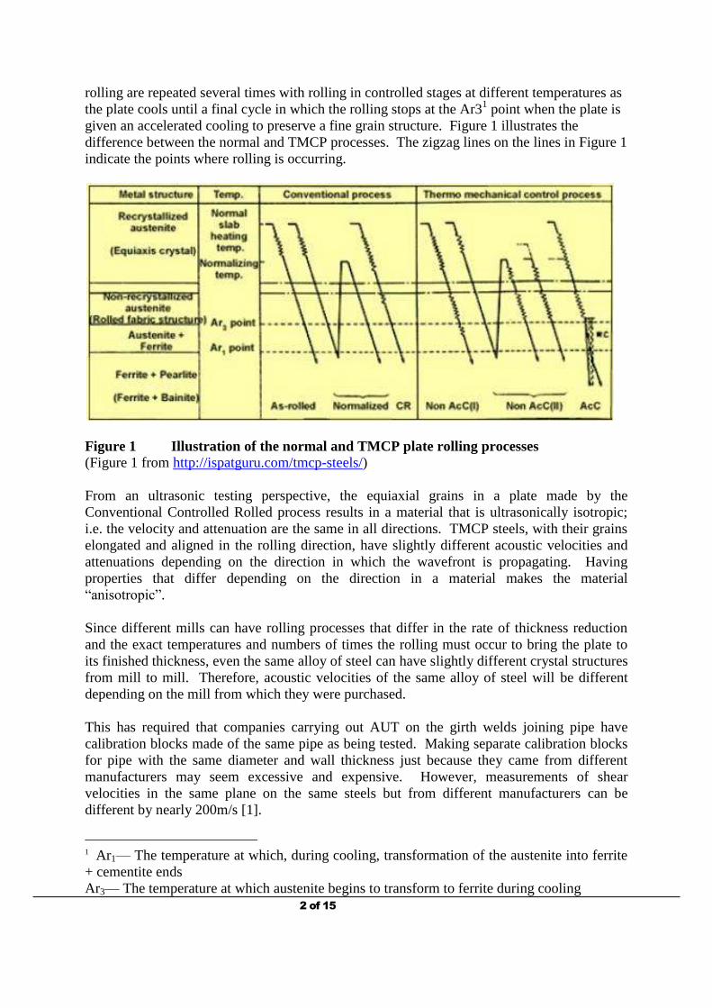
rolling are repeated several times with rolling in controlled stages at different temperatures as the plate cools until a final cycle in which the rolling stops at the Ar31 point when the plate is given an accelerated cooling to preserve a fine grain structure. Figure 1 illustrates the difference between the normal and TMCP processes. The zigzag lines on the lines in Figure 1 indicate the points where rolling is occurring.

Figure 1 Illustration of the normal and TMCP plate rolling processes (Figure 1 from http://ispatguru.com/tmcp-steels/) From an ultrasonic testing perspective, the equiaxial grains in a plate made by the Conventional Controlled Rolled process results in a material that is ultrasonically isotropic; i.e. the velocity and attenuation are the same in all directions. TMCP steels, with their grains elongated and aligned in the rolling direction, have slightly different acoustic velocities and attenuations depending on the direction in which the wavefront is propagating. Having properties that differ depending on the direction in a material makes the material “anisotropic”. Since different mills can have rolling processes that differ in the rate of thickness reduction and the exact temperatures and numbers of times the rolling must occur to bring the plate to its finished thickness, even the same alloy of steel can have slightly different crystal structures from mill to mill. Therefore, acoustic velocities of the same alloy of steel will be different depending on the mill from which they were purchased. This has required that companies carrying out AUT on the girth welds joining pipe have calibration blocks made of the same pipe as being tested. Making separate calibration blocks for pipe with the same diameter and wall thickness just because they came from different manufacturers may seem excessive and expensive. However, measurements of shear velocities in the same plane on the same steels but from different manufacturers can be different by nearly 200m/s [1].

1 Ar1— The temperature at which, during cooling, transformation of the austenite into ferrite + cementite ends Ar3— The temperature at which austenite begins to transform to ferrite during cooling

3 of 15

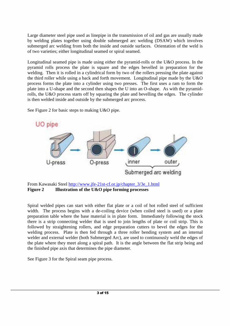
Large diameter steel pipe used as linepipe in the transmission of oil and gas are usually made by welding plates together using double submerged arc welding (DSAW) which involves submerged arc welding from both the inside and outside surfaces. Orientation of the weld is of two varieties; either longitudinal seamed or spiral seamed. Longitudinal seamed pipe is made using either the pyramid-rolls or the U&O process. In the pyramid rolls process the plate is square and the edges bevelled in preparation for the welding. Then it is rolled in a cylindrical form by two of the rollers pressing the plate against the third roller while using a back and forth movement. Longitudinal pipe made by the U&O process forms the plate into a cylinder using two presses. The first uses a ram to form the plate into a U-shape and the second then shapes the U into an O-shape. As with the pyramid-rolls, the U&O process starts off by squaring the plate and bevelling the edges. The cylinder is then welded inside and outside by the submerged arc process. See Figure 2 for basic steps to making U&O pipe.

From Kawasaki Steel http://www.jfe-21st-cf.or.jp/chapter_3/3e_1.html Figure 2 Illustration of the U&O pipe forming processes Spiral welded pipes can start with either flat plate or a coil of hot rolled steel of sufficient width. The process begins with a de-coiling device (when coiled steel is used) or a plate preparation table where the base material is in plate form. Immediately following the stock there is a strip connecting welder that is used to join lengths of plate or coil strip. This is followed by straightening rollers, and edge preparation cutters to bevel the edges for the welding process. Plate is then fed through a three roller bending system and an internal welder and external welder (both Submerged Arc), are used to continuously weld the edges of the plate where they meet along a spiral path. It is the angle between the flat strip being and the finished pipe axis that determines the pipe diameter. See Figure 3 for the Spiral seam pipe process.

4 of 15

From Kawasaki Steel http://www.jfe-21st-cf.or.jp/chapter_3/3e_1.html Figure 3 Illustration of the spiral welded pipe forming processes In the case where pipe is made using a longitudinal seam, the rolling direction of the plate is in the direction of the pipe axis. In the case where pipe is made using a spiral welded seam, the rolling direction will be at some angle to the pipe axis. Because some of the rolling occurs below the transition temperature in TMCP steels, the effect is to elongate and align the crystal structure in the direction of rolling is indicated in Figure 4.

Figure 4 Rolling plate to cause elongation and alignment of crystal structure When the plates are formed into pipe and joined with a girth weld, the ultrasonic inspection of the girth weld has the beam directed parallel to the elongated grains in the case of the longitudinal welded pipe. However, the beam is at some angle to the grains for spiral-seamed pipe (see Figure 5).

Figure 5 Grain orientation relative to girth weld axis for Long and Spiral seams

5 of 15

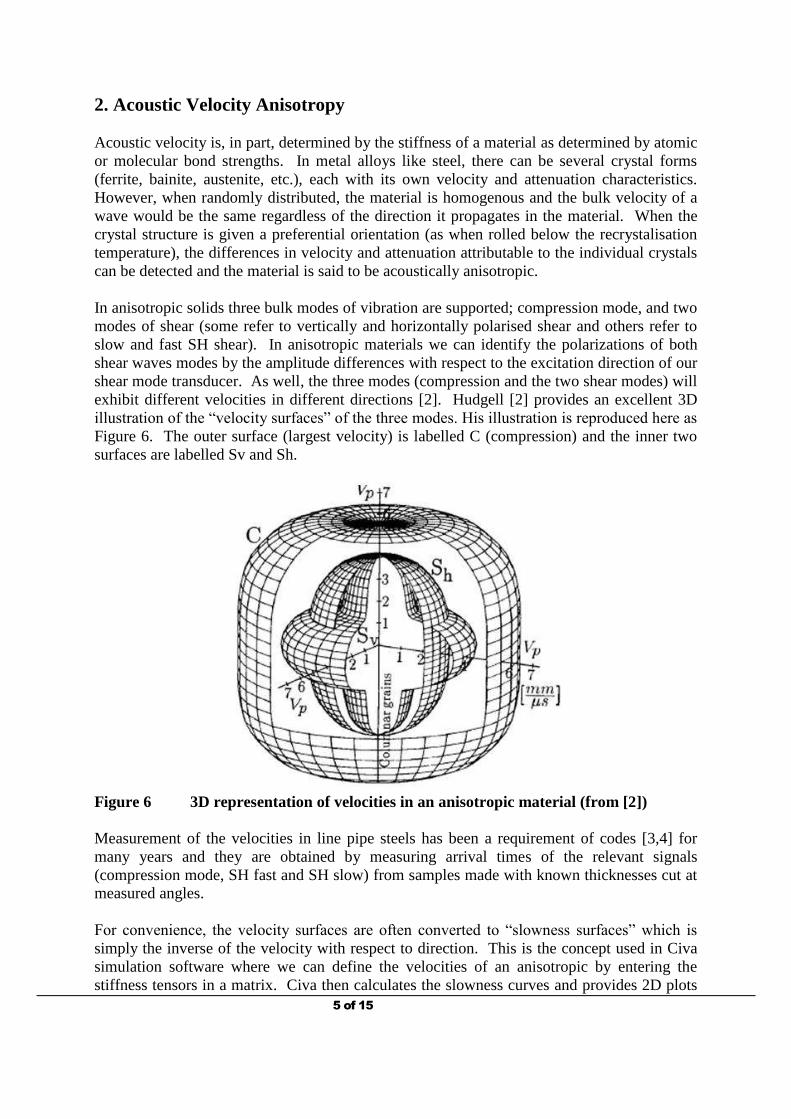
2. Acoustic Velocity Anisotropy Acoustic velocity is, in part, determined by the stiffness of a material as determined by atomic or molecular bond strengths. In metal alloys like steel, there can be several crystal forms (ferrite, bainite, austenite, etc.), each with its own velocity and attenuation characteristics. However, when randomly distributed, the material is homogenous and the bulk velocity of a wave would be the same regardless of the direction it propagates in the material. When the crystal structure is given a preferential orientation (as when rolled below the recrystalisation temperature), the differences in velocity and attenuation attributable to the individual crystals can be detected and the material is said to be acoustically anisotropic. In anisotropic solids three bulk modes of vibration are supported; compression mode, and two modes of shear (some refer to vertically and horizontally polarised shear and others refer to slow and fast SH shear). In anisotropic materials we can identify the polarizations of both shear waves modes by the amplitude differences with respect to the excitation direction of our shear mode transducer. As well, the three modes (compression and the two shear modes) will exhibit different velocities in different directions [2]. Hudgell [2] provides an excellent 3D illustration of the “velocity surfaces” of the three modes. His illustration is reproduced here as Figure 6. The outer surface (largest velocity) is labelled C (compression) and the inner two surfaces are labelled Sv and Sh.

Figure 6 3D representation of velocities in an anisotropic material (from [2]) Measurement of the velocities in line pipe steels has been a requirement of codes [3,4] for many years and they are obtained by measuring arrival times of the relevant signals (compression mode, SH fast and SH slow) from samples made with known thicknesses cut at measured angles. For convenience, the velocity surfaces are often converted to “slowness surfaces” which is simply the inverse of the velocity with respect to direction. This is the concept used in Civa simulation software where we can define the velocities of an anisotropic by entering the stiffness tensors in a matrix. Civa then calculates the slowness curves and provides 2D plots

6 of 15

in the three perpendicular planes and also provides a 3D image of the curves that can be over-laid in the models. Figure 7 illustrates the 2D “slowness curves” provided by Civa for an imaginary anisotropic material. From left to right we have the XY plane, YZ plane and the ZX plane. The Green curve indicates the compression mode and the other (slower) curves are the fast and slow shear curves. Civa 2D plots indicate the slower shear mode in the orange colour and the faster shear mode in pink. In the middle image of Figure 7 (YZ plane) we see the apparent crossing of the slow and fast modes. However, when plotted, the colours change such that the outer curve is always orange and the inner always pink.

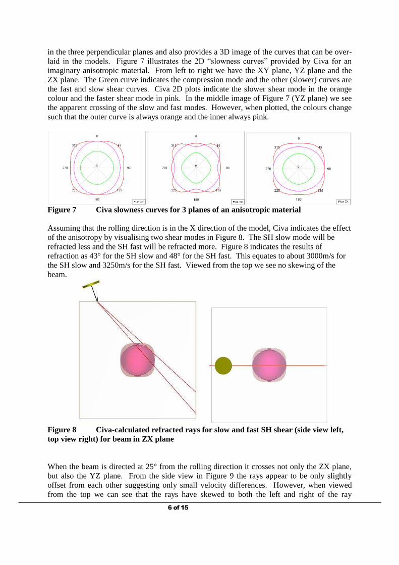
Figure 7 Civa slowness curves for 3 planes of an anisotropic material Assuming that the rolling direction is in the X direction of the model, Civa indicates the effect of the anisotropy by visualising two shear modes in Figure 8. The SH slow mode will be refracted less and the SH fast will be refracted more. Figure 8 indicates the results of refraction as 43° for the SH slow and 48° for the SH fast. This equates to about 3000m/s for the SH slow and 3250m/s for the SH fast. Viewed from the top we see no skewing of the beam.

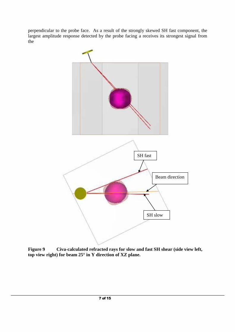
Figure 8 Civa-calculated refracted rays for slow and fast SH shear (side view left, top view right) for beam in ZX plane When the beam is directed at 25° from the rolling direction it crosses not only the ZX plane, but also the YZ plane. From the side view in Figure 9 the rays appear to be only slightly offset from each other suggesting only small velocity differences. However, when viewed from the top we can see that the rays have skewed to both the left and right of the ray

7 of 15

perpendicular to the probe face. As a result of the strongly skewed SH fast component, the largest amplitude response detected by the probe facing a receives its strongest signal from the

Figure 9 Civa-calculated refracted rays for slow and fast SH shear (side view left, top view right) for beam 25° in Y direction of XZ plane.

Beam direction

SH fast

SH slow

8 of 15

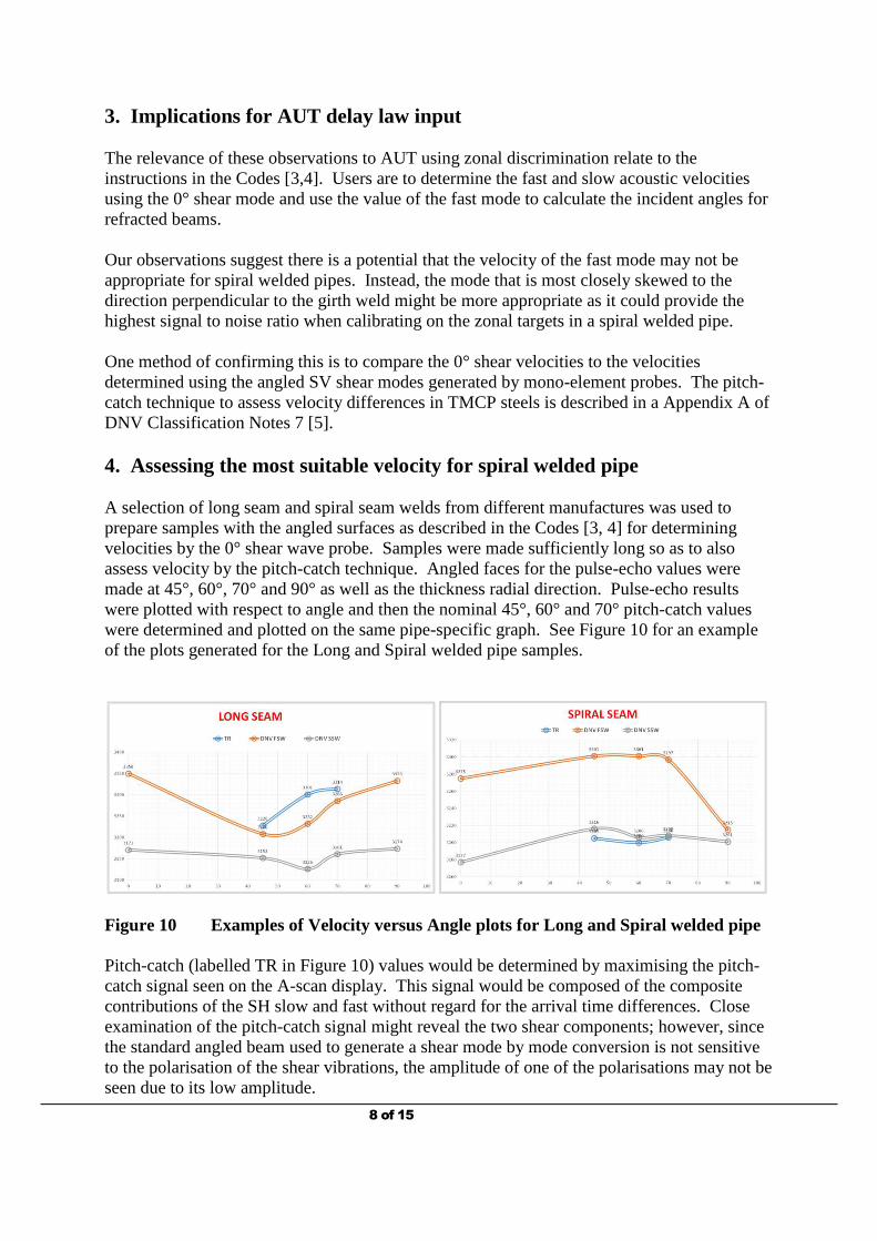
3. Implications for AUT delay law input The relevance of these observations to AUT using zonal discrimination relate to the instructions in the Codes [3,4]. Users are to determine the fast and slow acoustic velocities using the 0° shear mode and use the value of the fast mode to calculate the incident angles for refracted beams. Our observations suggest there is a potential that the velocity of the fast mode may not be appropriate for spiral welded pipes. Instead, the mode that is most closely skewed to the direction perpendicular to the girth weld might be more appropriate as it could provide the highest signal to noise ratio when calibrating on the zonal targets in a spiral welded pipe. One method of confirming this is to compare the 0° shear velocities to the velocities determined using the angled SV shear modes generated by mono-element probes. The pitch-catch technique to assess velocity differences in TMCP steels is described in a Appendix A of DNV Classification Notes 7 [5]. 4. Assessing the most suitable velocity for spiral welded pipe A selection of long seam and spiral seam welds from different manufactures was used to prepare samples with the angled surfaces as described in the Codes [3, 4] for determining velocities by the 0° shear wave probe. Samples were made sufficiently long so as to also assess velocity by the pitch-catch technique. Angled faces for the pulse-echo values were made at 45°, 60°, 70° and 90° as well as the thickness radial direction. Pulse-echo results were plotted with respect to angle and then the nominal 45°, 60° and 70° pitch-catch values were determined and plotted on the same pipe-specific graph. See Figure 10 for an example of the plots generated for the Long and Spiral welded pipe samples.

Figure 10 Examples of Velocity versus Angle plots for Long and Spiral welded pipe Pitch-catch (labelled TR in Figure 10) values would be determined by maximising the pitch-catch signal seen on the A-scan display. This signal would be composed of the composite contributions of the SH slow and fast without regard for the arrival time differences. Close examination of the pitch-catch signal might reveal the two shear components; however, since the standard angled beam used to generate a shear mode by mode conversion is not sensitive to the polarisation of the shear vibrations, the amplitude of one of the polarisations may not be seen due to its low amplitude.

9 of 15

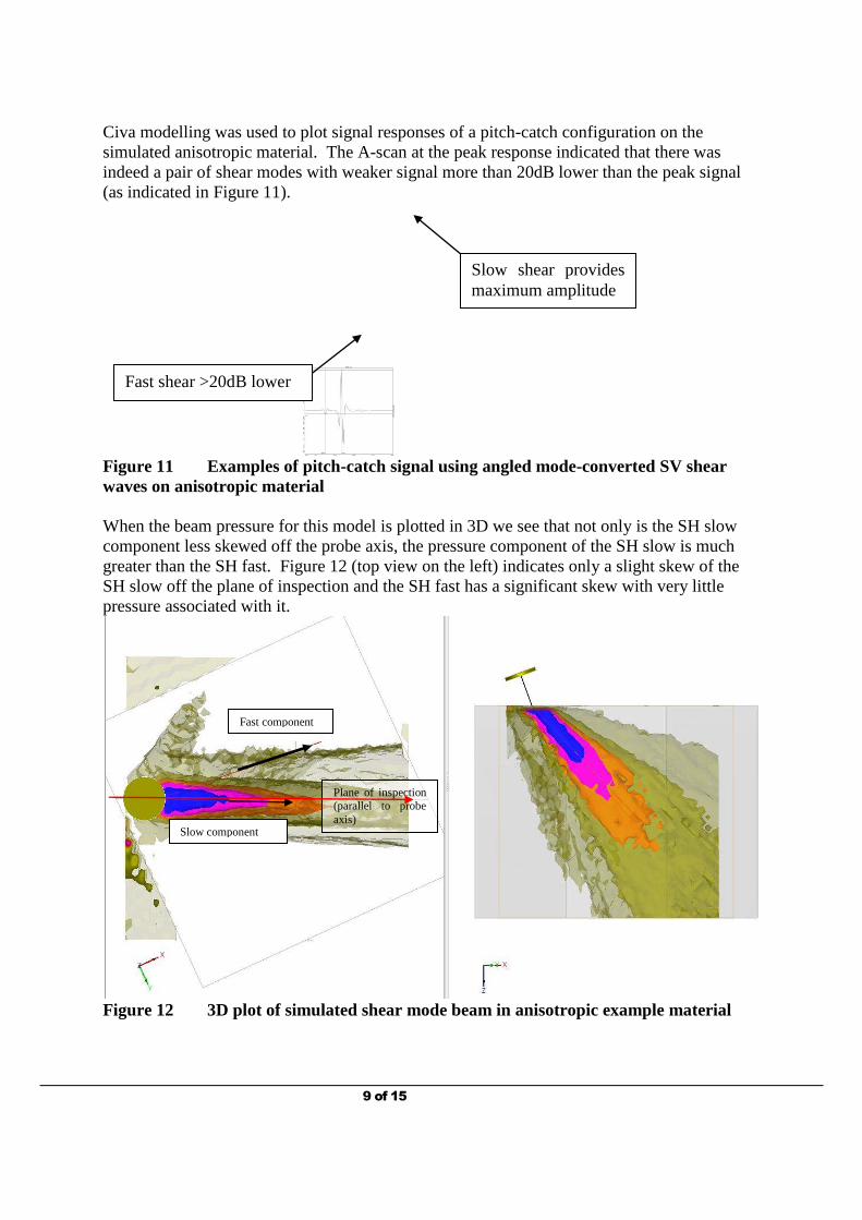
Civa modelling was used to plot signal responses of a pitch-catch configuration on the simulated anisotropic material. The A-scan at the peak response indicated that there was indeed a pair of shear modes with weaker signal more than 20dB lower than the peak signal (as indicated in Figure 11).

Figure 11 Examples of pitch-catch signal using angled mode-converted SV shear waves on anisotropic material When the beam pressure for this model is plotted in 3D we see that not only is the SH slow component less skewed off the probe axis, the pressure component of the SH slow is much greater than the SH fast. Figure 12 (top view on the left) indicates only a slight skew of the SH slow off the plane of inspection and the SH fast has a significant skew with very little pressure associated with it.

Figure 12 3D plot of simulated shear mode beam in anisotropic example material

Fast shear >20dB lower

Slow shear provides maximum amplitude

Fast component

Slow component

Plane of inspection (parallel to probe axis)

10 of 15

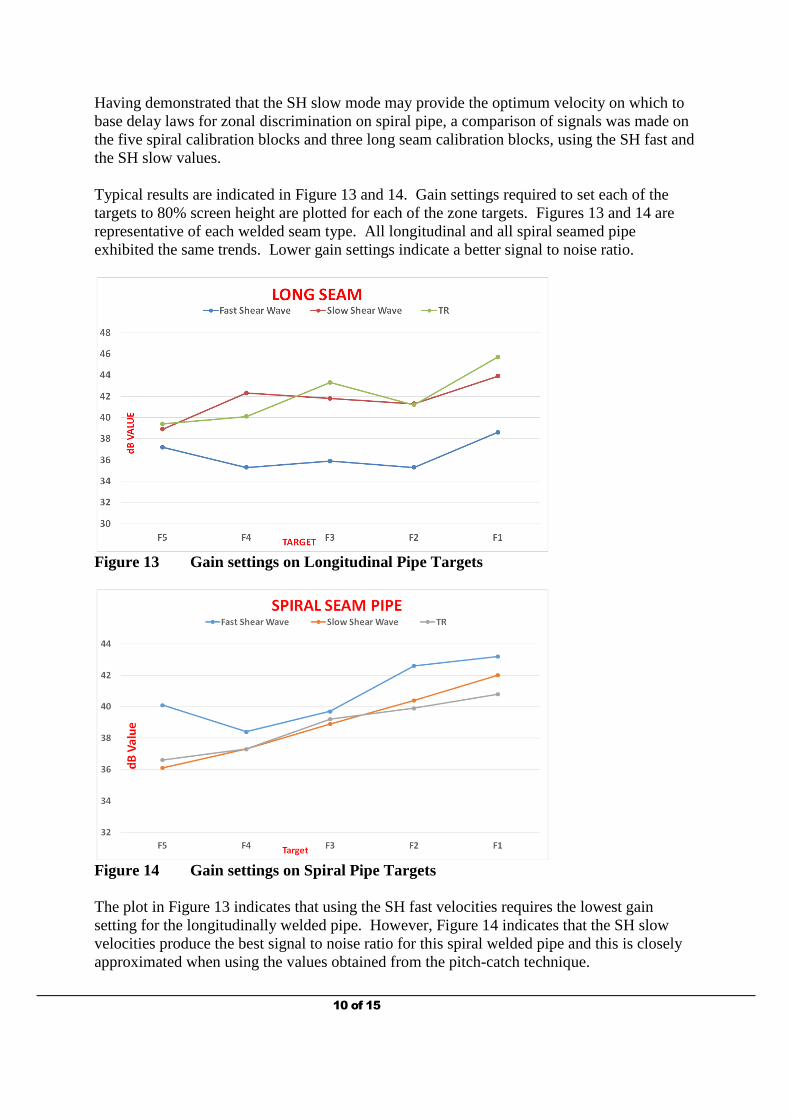
Having demonstrated that the SH slow mode may provide the optimum velocity on which to base delay laws for zonal discrimination on spiral pipe, a comparison of signals was made on the five spiral calibration blocks and three long seam calibration blocks, using the SH fast and the SH slow values. Typical results are indicated in Figure 13 and 14. Gain settings required to set each of the targets to 80% screen height are plotted for each of the zone targets. Figures 13 and 14 are representative of each welded seam type. All longitudinal and all spiral seamed pipe exhibited the same trends. Lower gain settings indicate a better signal to noise ratio.

Figure 13 Gain settings on Longitudinal Pipe Targets

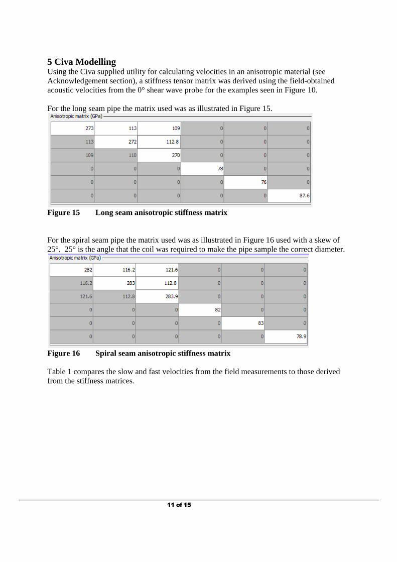
Figure 14 Gain settings on Spiral Pipe Targets The plot in Figure 13 indicates that using the SH fast velocities requires the lowest gain setting for the longitudinally welded pipe. However, Figure 14 indicates that the SH slow velocities produce the best signal to noise ratio for this spiral welded pipe and this is closely approximated when using the values obtained from the pitch-catch technique.

11 of 15

5 Civa Modelling Using the Civa supplied utility for calculating velocities in an anisotropic material (see Acknowledgement section), a stiffness tensor matrix was derived using the field-obtained acoustic velocities from the 0° shear wave probe for the examples seen in Figure 10. For the long seam pipe the matrix used was as illustrated in Figure 15.

Figure 15 Long seam anisotropic stiffness matrix For the spiral seam pipe the matrix used was as illustrated in Figure 16 used with a skew of 25°. 25° is the angle that the coil was required to make the pipe sample the correct diameter.

Figure 16 Spiral seam anisotropic stiffness matrix Table 1 compares the slow and fast velocities from the field measurements to those derived from the stiffness matrices.

12 of 15

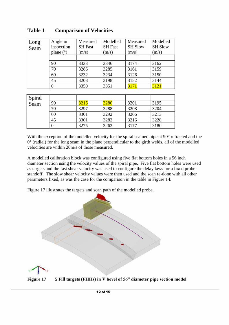
Table 1 Comparison of Velocities Long Seam

Angle in inspection plane (°)

Measured SH Fast (m/s)

Modelled SH Fast (m/s)

Measured SH Slow (m/s)

Modelled SH Slow (m/s)

90 3333 3346 3174 3162 70 3286 3285 3161 3159 60 3232 3234 3126 3150 45 3208 3198 3152 3144 0 3350 3351 3171 3121

Spiral Seam

90 3215 3280 3201 3195 70 3297 3288 3208 3204 60 3301 3292 3206 3213 45 3301 3282 3216 3228 0 3275 3262 3177 3180

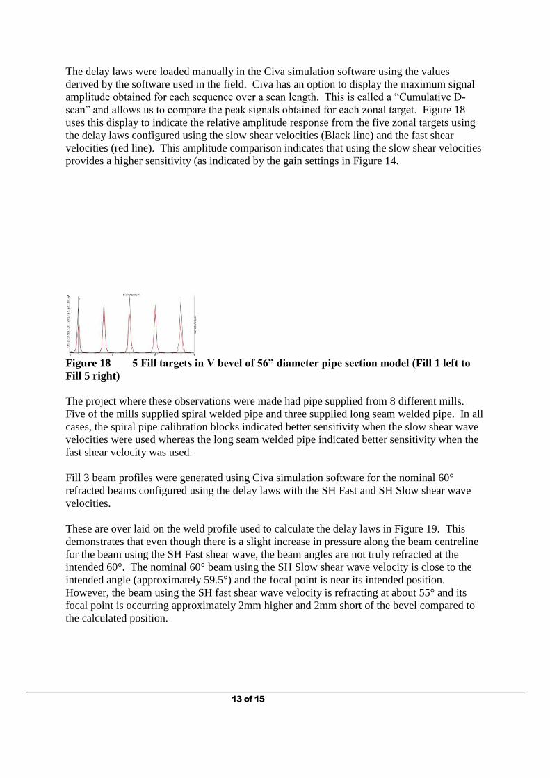
With the exception of the modelled velocity for the spiral seamed pipe at 90° refracted and the 0° (radial) for the long seam in the plane perpendicular to the girth welds, all of the modelled velocities are within 20m/s of those measured. A modelled calibration block was configured using five flat bottom holes in a 56 inch diameter section using the velocity values of the spiral pipe. Five flat bottom holes were used as targets and the fast shear velocity was used to configure the delay laws for a fixed probe standoff. The slow shear velocity values were then used and the scan re-done with all other parameters fixed, as was the case for the comparison in the table in Figure 14. Figure 17 illustrates the targets and scan path of the modelled probe.

Figure 17 5 Fill targets (FHHs) in V bevel of 56” diameter pipe section model

13 of 15

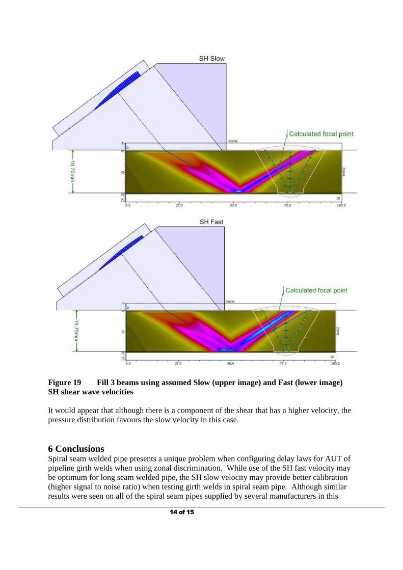
The delay laws were loaded manually in the Civa simulation software using the values derived by the software used in the field. Civa has an option to display the maximum signal amplitude obtained for each sequence over a scan length. This is called a “Cumulative D-scan” and allows us to compare the peak signals obtained for each zonal target. Figure 18 uses this display to indicate the relative amplitude response from the five zonal targets using the delay laws configured using the slow shear velocities (Black line) and the fast shear velocities (red line). This amplitude comparison indicates that using the slow shear velocities provides a higher sensitivity (as indicated by the gain settings in Figure 14.

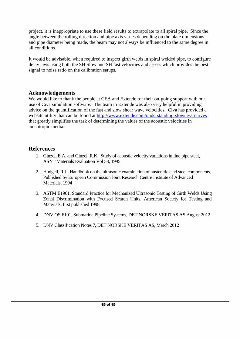
Figure 18 5 Fill targets in V bevel of 56” diameter pipe section model (Fill 1 left to Fill 5 right) The project where these observations were made had pipe supplied from 8 different mills. Five of the mills supplied spiral welded pipe and three supplied long seam welded pipe. In all cases, the spiral pipe calibration blocks indicated better sensitivity when the slow shear wave velocities were used whereas the long seam welded pipe indicated better sensitivity when the fast shear velocity was used. Fill 3 beam profiles were generated using Civa simulation software for the nominal 60° refracted beams configured using the delay laws with the SH Fast and SH Slow shear wave velocities. These are over laid on the weld profile used to calculate the delay laws in Figure 19. This demonstrates that even though there is a slight increase in pressure along the beam centreline for the beam using the SH Fast shear wave, the beam angles are not truly refracted at the intended 60°. The nominal 60° beam using the SH Slow shear wave velocity is close to the intended angle (approximately 59.5°) and the focal point is near its intended position. However, the beam using the SH fast shear wave velocity is refracting at about 55° and its focal point is occurring approximately 2mm higher and 2mm short of the bevel compared to the calculated position.

14 of 15

Figure 19 Fill 3 beams using assumed Slow (upper image) and Fast (lower image) SH shear wave velocities It would appear that although there is a component of the shear that has a higher velocity, the pressure distribution favours the slow velocity in this case. 6 Conclusions Spiral seam welded pipe presents a unique problem when configuring delay laws for AUT of pipeline girth welds when using zonal discrimination. While use of the SH fast velocity may be optimum for long seam welded pipe, the SH slow velocity may provide better calibration (higher signal to noise ratio) when testing girth welds in spiral seam pipe. Although similar results were seen on all of the spiral seam pipes supplied by several manufacturers in this

15 of 15

project, it is inappropriate to use these field results to extrapolate to all spiral pipe. Since the angle between the rolling direction and pipe axis varies depending on the plate dimensions and pipe diameter being made, the beam may not always be influenced to the same degree in all conditions. It would be advisable, when required to inspect girth welds in spiral welded pipe, to configure delay laws using both the SH Slow and SH fast velocities and assess which provides the best signal to noise ratio on the calibration setups. Acknowledgements We would like to thank the people at CEA and Extende for their on-going support with our use of Civa simulation software. The team in Extende was also very helpful in providing advice on the quantification of the fast and slow shear wave velocities. Civa has provided a website utility that can be found at http://www.extende.com/understanding-slowness-curves that greatly simplifies the task of determining the values of the acoustic velocities in anisotropic media.

References 1. Ginzel, E.A. and Ginzel, R.K., Study of acoustic velocity variations in line pipe steel,

ASNT Materials Evaluation Vol 53, 1995

2. Hudgell, R.J., Handbook on the ultrasonic examination of austenitic clad steel components, Published by European Commission Joint Research Centre Institute of Advanced Materials, 1994

3. ASTM E1961, Standard Practice for Mechanized Ultrasonic Testing of Girth Welds Using Zonal Discrimination with Focused Search Units, American Society for Testing and Materials, first published 1998

4. DNV OS F101, Submarine Pipeline Systems, DET NORSKE VERITAS AS August 2012

5. DNV Classification Notes 7, DET NORSKE VERITAS AS, March 2012