Ad Hoc Synchronization

8/6/2019 Ad Hoc Synchronization

http://slidepdf.com/reader/full/ad-hoc-synchronization 1/9

Time Synchronization in Ad Hoc Networks

Kay RomerDepartment of Computer Science

ETH Zurich8092 Zurich, Switzerland

[email protected]

ABSTRACTUbiquitous computing environments are typically based upon ad

hoc networks of mobile computing devices. These devices may be

equipped with sensor hardware to sense the physical environment

and may be attached to real world artifacts to form so–called smart

things. The data sensed by various smart things can then be com-

bined to derive knowledge about the environment, which in turn

enables the smart things to “react” intelligently to their environ-

ment. For this so–called sensor fusion, temporal relationships (X

happened before Y) and real–time issues (X and Y happened within

a certain time interval) play an important role. Thus physical time

and clock synchronization are crucial in such environments. How-

ever, due to the characteristics of sparse ad hoc networks, classical

clock synchronization algorithms are not applicable in this setting.

We present a time synchronization scheme that is appropriate for

sparse ad hoc networks.

Keywordstime synchronization, clock synchronization, ad hoc networks,

spontaneous networking, ubiquitous computing, sensor fusion,

smart things

1. INTRODUCTIONConsider ubiquitous computing scenarios where everyday things

(such as watches, coffee cups, books) are made “smart” by attach-

ing small computing devices to them that are able to sense the phys-

ical environment (e.g., location, illumination, temperature, acceler-

ation) and are able to communicate via short range radio with each

other. Such smart things are spontaneously networked: if they are

brought into the vicinity of one another, a communication link is es-

tablished, which is removed again when the smart things are moved

away from each other. In general, communication links are rather

short lived and the resulting network of smart things is highly dy-

namic.

In such a setting, one often wants to reason about the “real world”

(the environment of the smart things) as sensed by smart artifacts.

The idea is to combine the information collected about the environ-

ment by the individual smart things into some higher level infor-

mation or knowledge [4, 7, 8, 11] also known as sensor fusion.

Consider for example environment monitoring systems, which in-

volve the detection of direction and speed of certain phenomena

such as fire, oil slicks, water pollution, or animal herds. Mobile

computing devices equipped with sensors, clocks, and short range

radio are deployed in the environment (e.g., dropped into water,

or attached to animals). The devices record the time when they

detect or no longer detect the phenomenon and communicate this

information to other devices as they pass by. In order to determine

the direction of the phenomenon, temporal ordering of these events

originating from different devices (and thus different clocks) has

to be determined. To estimate the speed of the phenomenon time

differences between events originating from different devices have

to be calculated.

Time synchronization is also useful for estimating proximity of and

distances between smart things by taking into account the points in

time when a certain phenomenon in the environment (e.g., sound,

light, air pressure) is sensed by different smart things.

These examples indicate that temporal ordering and other real–

time1 issues play an important role in such environments. As we

will see later, neither logical time [12, 14] nor classical physical

clock synchronization algorithms [3, 13, 16, 17] can be used tosolve this problem in general. We will suggest an algorithm that

solves the temporal ordering problem and other real–time issues in

environments sketched above.

2. AD HOC NETWORKSAd hoc networks [2] are networks of mobile wireless computing

devices. Due to the limited communication range of wireless tech-

nology (about 10 meters for Bluetooth [1]), nodes of the network

form spontaneous connections when they are brought within the

communication range of each other, providing typically a symmet-

rical communication link where message exchange is possible in

both directions. The limited communication range and the mobility

of the nodes lead to frequent reconfiguration of the network topol-

ogy.

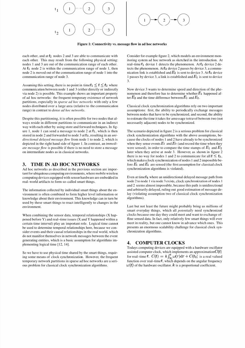
The left hand side of figure 1 shows the configurations (topologies)

of an ad hoc network consisting of three nodes at two points in

time ¡ £¥ § ¦

. At ¡

nodes 1 and 2 are able to communicate with¡

Throughout the paper the term real–time refers to UTC.



t

t

1

2

1

1

1

2 3

2 3

2 3

Figure 1: Connectivity vs. message flow in ad hoc networks

each other, and at ¦

nodes 2 and 3 are able to communicate with

each other. This may result from the following physical setting:nodes 1 and 3 are out of the communication range of each other.

At ¡

node 2 is within the communication range of node 1, then

node 2 is moved out of the communication range of node 1 into the

communication range of node 3.

Assuming this setting, there is no point in time ¡

¡

¡ ¦

where

communication between node 1 and 3 (either directly or indirectly

via node 2) is possible. This example shows an important property

of ad hoc networks: the frequent temporary existence of network

partitions, especially in sparse ad hoc networks with only a few

nodes distributed over a large area (relative to the communication

range) in contrast to dense ad hoc networks.

Despite this partitioning, it is often possible for two nodes that al-

ways reside in different partitions to communicate in an indirectway with each other by using store and forward techniques. In fig-

ure 1, node 1 can send a message to node 2 at

¡

, which is then

stored in node 2 and forwarded to node 3 at ¦

, resulting in an uni-

directional delayed message flow from node 1 to node 2, which is

depicted in the right hand side of figure 1. In contrast, an immedi-

ate message flow is possible if there is no need to store a message

on intermediate nodes as in classical networks.

3. TIME IN AD HOC NETWORKSAd hoc networks as described in the previous section are impor-

tant for ubiquitous computing environments, where mobile wireless

computing devices equipped with sensor hardware are embedded in

real–world artifacts to form so–called smart things.

The information collected by individual smart things about the en-

vironment is often combined to form higher level information or

knowledge about their environment. This knowledge can in turn be

used by these smart things to react intelligently to changes in the

environment.

When combining the sensor data, temporal relationships (X hap-

pened before Y) and real–time issues (X and Y happened within a

certain time interval) play an important role. Logical time cannot

be used to determine temporal relationships here, because we con-

sider events and their causal relationships in the real world, which

do not manifest themselves in network messages between the event

generating entities, which is a basic assumption for algorithms im-

plementing logical time [12, 14].

So we have to use physical time shared by the smart things, requir-

ing some means of clock synchronization. However, the frequent

temporary network partitions in sparse ad hoc networks are a seri-

ous problem for classical clock synchronization algorithms.

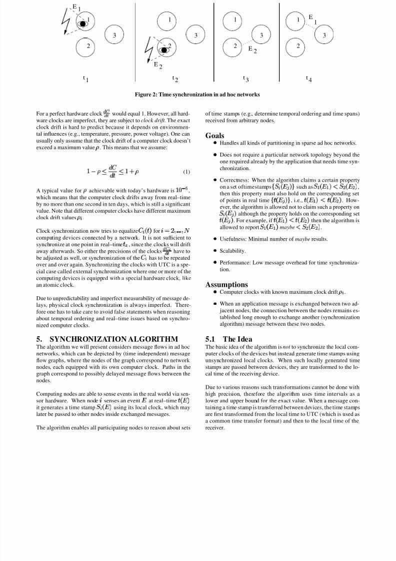
Consider for example figure 2, which models an environment mon-

itoring system ad hoc network as sketched in the introduction. Atreal–time

¡

device 1 detects the phenomenon. At

¦

device 2 de-

tects the phenomenon. At ¢

device 2 passes by device 3, a commu-

nication link is established and ¤

¦

is sent to device 3. At ¥

device

1 passes by device 3, a link is established and¤

¡

is sent to device

3.

Now device 3 wants to determine speed and direction of the phe-

nomenon and therefore has to determine whether ¤

¡

happened af-

ter ¤

¦

and the time difference between ¤

¡

and ¤

¦

.

Classical clock synchronization algorithms rely on two important

assumptions: first, the ability to periodically exchange messages

between nodes that have to be synchronized, and second, the ability

to estimate the time it takes for amessage totravel between two (not

necessarily adjacent) nodes to be synchronized.

The scenario depicted in figure 2 is a serious problem for classical

clock synchronization algorithms with the above assumptions, be-

cause the clocks of nodes 1 and 2 have already to be synchronized

when they sense events ¤

¡

and ¤

¦

(and record the time when they

were sensed), in order to compare the time stamps of ¤

¡

and ¤

¦

later when they arrive at node 3. However, as shown in figure 2

there is no way for nodes 1 and 2 to communicate for all

¡

¢

,

which makes clock synchronization of nodes 1 and 2 impossible be-

fore¤

¡

and¤

¦

are sensed (the first assumption for classical clock

synchronization algorithms is violated).

Even at time ¥

where an unidirectional delayed message path from

node 2 to node 1 via node 3 exists, clock synchronization of nodes 1and 2 seems almost impossible, because this path is unidirectional

and arbitrarily delayed, ruling out good estimation of message de-

lay (violating assumption two of classical clock synchronization

algorithms).

Last but not least the future might probably bring us millions of

smart everyday things, which all potentially need synchronized

clocks because one day they could meet and want to exchange of-

fline sensed data. In fact, only relatively few smart things will ever

meet in reality, but one cannot know in advance which ones. This

presents an enormous scalability challenge for classical clock syn-

chronization algorithms.

4. COMPUTER CLOCKSTodays computing devices are equipped with a hardware oscillator

assisted computer clock, which implements an approximation ¦ §

©

for real–time

. ¦ §

©

!

§ #

© %

# ' ¦ §

0 ©

is a real valued

function over real–time

, which depends on the angular frequency

!

§

©

of the hardware oscillator.

is a proportional coefficient.



1

2

E1

3

1

2

E2

3

1

2

3

E2

1

2

3

E1

t1

t2

t3

t4

Figure 2: Time synchronization in ad hoc networks

For a perfect hardware clock

¡

would equal 1. However, all hard-

ware clocks are imperfect, they are subject to clock drift . The exact

clock drift is hard to predict because it depends on environmen-

tal influences (e.g., temperature, pressure, power voltage). One can

usually only assume that the clock drift of a computer clock doesn’t

exceed a maximum value ¢ . This means that we assume:

£ ¤

¢

¡ ¦¦

¦

¡£

' ¢ (1)

A typical value for¢

achievable with today’s hardware is£ ©

,

which means that the computer clock drifts away from real–timeby no more than one second in ten days, which is still a significant

value. Note that different computer clocks have different maximum

clock drift values ¢ .

Clock synchronization now tries to equalize¦ §

©

for

" " " &

computing devices connected by a network. It is not sufficient to

synchronize at one point in real–time (

, since the clocks will drift

away afterwards. So either the precisions of the clocks

¡ 0

have to

be adjusted as well, or synchronization of the ¦ has to be repeated

over and over again. Synchronizing the clocks with UTC is a spe-

cial case called external synchronization where one or more of the

computing devices is equipped with a special hardware clock, like

an atomic clock.

Due to unpredictability and imperfect measurability of message de-

lays, physical clock synchronization is always imperfect. There-

fore one has to take care to avoid false statements when reasoning

about temporal ordering and real–time issues based on synchro-

nized computer clocks.

5. SYNCHRONIZATION ALGORITHMThe algorithm we will present considers message flows in ad hoc

networks, which can be depicted by (time independent) message

flow graphs, where the nodes of the graph correspond to network

nodes, each equipped with its own computer clock. Paths in the

graph correspond to possibly delayed message flows between the

nodes.

Computing nodes are able to sense events in the real world via sen-sor hardware. When node

senses an event

¤at real–time

§ ¤

©

it generates a time stamp 2 § ¤

©

using its local clock, which may

later be passed to other nodes inside exchanged messages.

The algorithm enables all participating nodes to reason about sets

of time stamps (e.g., determine temporal ordering and time spans)

received from arbitrary nodes.

Goals4

Handles all kinds of partitioning in sparse ad hoc networks.4

Does not require a particular network topology beyond the

one required already by the application that needs time syn-

chronization.4

Correctness: When the algorithm claims a certain property

on a set oftimestamps5 2 § ¤ 7

© 9

such as2

¡

§ ¤

¡

© £

2

¦

§ ¤

¦

©

,

then this property must also hold on the corresponding set

of points in real time5

§ ¤7

© 9

, i.e.,

§ ¤

¡ © £

§ ¤

¦ ©

. How-

ever, the algorithm is allowed not to claim such a property on

2

§ ¤7

©

although the property holds on the corresponding set

§ ¤ 7

©

. For example, if

§ ¤

¡ © £

§ ¤

¦ ©

then the algorithm is

allowed to report2

¡

§ ¤

¡ ©

maybe£

2

¦

§ ¤

¦ ©

.4

Usefulness: Minimal number of maybe results.4

Scalability.4

Performance: Low message overhead for time synchroniza-

tion.

Assumptions4

Computer clocks with known maximum clock drift¢

.4

When an application message is exchanged between two ad-

jacent nodes, the connection between the nodes remains es-

tablished long enough to exchange another (synchronization

algorithm) message between these two nodes.

5.1 The IdeaThe basic idea of the algorithm is not to synchronize the local com-

puter clocks of the devices but instead generate time stamps using

unsynchronized local clocks. When such locally generated time

stamps are passed between devices, they are transformed to the lo-

cal time of the receiving device.

Due to various reasons such transformations cannot be done with

high precision, therefore the algorithm uses time intervals as alower and upper bound for the exact value. When a message con-

taining a time stamp is transferred between devices, the time stamps

are first transformed from the local time to UTC (which is used as

a common time transfer format) and then to the local time of the

receiver.



Receiver

Sender

Time in Receiver

Time in Sender

t t t

t t t4 5 6

1 2 3

M MACK ACK1 21 2

Figure 3: Message delay estimation

Stated in more detail, the algorithm determines lower and upper

bounds for the real–time passed from generation of the time stamp

in the source node to arrival of the message in the destination node,

transforms these bounds to the time of the receiver and subtracts

the resulting values from the time of arrival in the destination node.

The resulting interval specifies lower and upper bounds for the time

stamp relative to the local time of the receiving node.

5.2 Time TransformationAs we will see in the following section, transforming real–time dif-

ferences

into computer clock differences ¦ and vice versa is

at the heart of the algorithm. These transformations cannot be done

exactly due to the unpredictability of the computer clocks, but will

result in estimates (lower and upper bounds). Basis for the trans-formation is the difference based version of inequality 1:

£ ¤

¢

¡ ¦

¡ £

' ¢(2)

which can be transformed into§

£ ¤

¢

©

¡

¦

¡

§

£

' ¢

©

and ¡

¡

¡ ¢ ¤

¡

¡

¡

¡

¡

¤ , which means that we can approximate the

computer clock difference ¦

that corresponds to the real–time

difference

by the interval ¦§

£ ¤

¢

©

§

£

' ¢

©

§

. Vice versa

the real–time difference

that corresponds to the computer clock

difference ¦ can be approximated by the interval ¦

¡

¡

¡ ¢ ¤

¡

¡

¡

¤

§

accordingly.

In order to transform a time difference ¦

from the local

time of one node (with¢

¡

) to the local time of a different

node (with ¢

¦

), ¦ is first estimated by the real–time interval

¦¡

¡

¡ ¢ ¤

¡

¡

¡

¤

§

, which in turn is estimated by the computer time

interval ¦ ¦

¡

¤

¡ ¢ ¤

¦

¡ ¢ ¤

¡

¤

§

relative to the local time of node 2.

5.3 Message DelayAs pointed out above, the algorithm will determine estimations for

the lifetime of a time stamp. For this it has to know estimations

for the message delay ¦ of messages sent between adjacent nodes.

Since we cannot assume a constant message delay due to the highly

dynamic characteristics of ad hoc networks, message delay has to

be measured for each transferred message in order to achieve the

correctness goal.

One important observation is that a message transfer between two

nodes is often accomplished by sending two messages, the message

that is to be transferred from the sender to the receiver and an ac-

knowledgment back from the receiver to the sender to inform the

sender of the successful arrival of the message. Thus, it is possi-

ble to measure the round trip time

(time passed from sending

the message in the sender to arrival of the acknowledgment in the

sender) using the local clock of the sender. The message delay can

then be estimated by the the lower bound©

and the upper bound

. Now the sender knows an estimation for the message delay,

but in our algorithm the receiving side has to know this approxima-

tion in order to update the received time stamp. Transferring the

estimation from the sender to the receiver would take another pair

of messages (one for passing the estimation from sender to receiver

and an ack back to the sender to inform the sender of the success-

ful arrival of the message), which would result in 100% message

overhead.

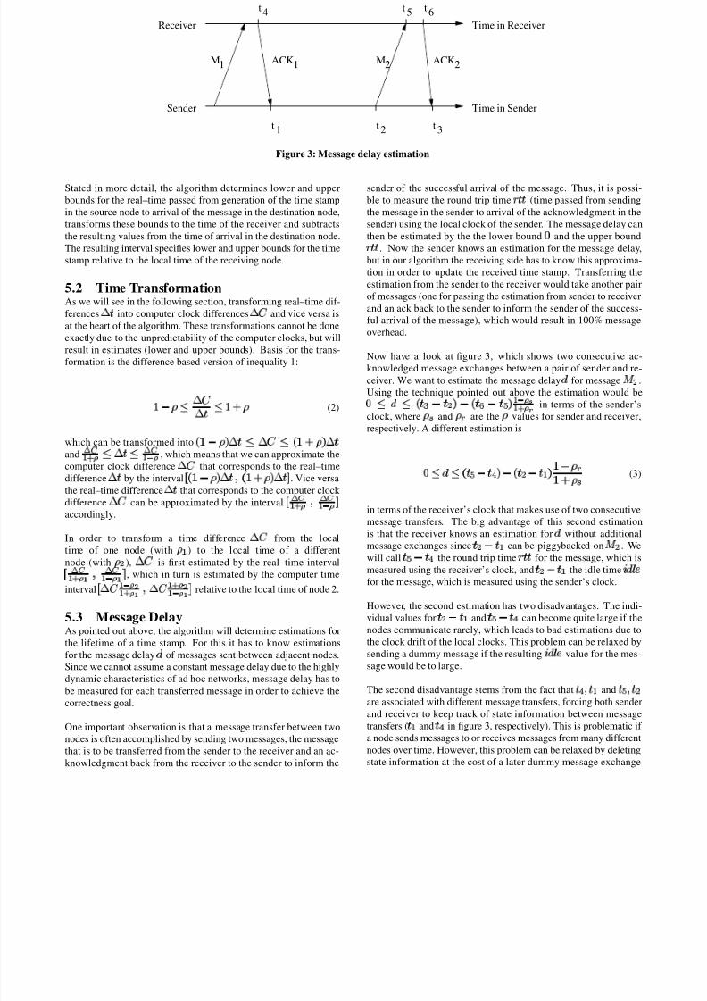
Now have a look at figure 3, which shows two consecutive ac-

knowledged message exchanges between a pair of sender and re-

ceiver. We want to estimate the message delay ¦ for message

¦

.

Using the technique pointed out above the estimation would be©

¡

¦

¡

§

¢

¤

¦

©

¤

§

¤

©

¡

¤

¡ ¢ ¤ in terms of the sender’s

clock, where ¢ " and ¢ $ are the ¢ values for sender and receiver,

respectively. A different estimation is

©¡

¦

¡

§

¤

¥ ©

¤

§

¦

¤

¡ ©

£ ¤

¢ $

£

' ¢"

(3)

in terms of the receiver’s clock that makes use of two consecutive

message transfers. The big advantage of this second estimationis that the receiver knows an estimation for ¦ without additional

message exchanges since

¦

¤

¡

can be piggybacked on

¦

. We

will call

¤

¥

the round trip time

for the message, which is

measured using the receiver’s clock, and

¦

¤

¡

the idle time ¦ & (

for the message, which is measured using the sender’s clock.

However, the second estimation has two disadvantages. The indi-

vidual values for ¦

¤

¡

and

¤

¥

can become quite large if the

nodes communicate rarely, which leads to bad estimations due to

the clock drift of the local clocks. This problem can be relaxed by

sending a dummy message if the resulting

¦ & ( value for the mes-

sage would be to large.

The second disadvantage stems from the fact that ¥

¡

and

¦

are associated with different message transfers, forcing both senderand receiver to keep track of state information between message

transfers ( ¡

and ¥

in figure 3, respectively). This is problematic if

a node sends messages to or receives messages from many different

nodes over time. However, this problem can be relaxed by deleting

state information at the cost of a later dummy message exchange



to reinitialize the clock values, for example in a least recently used

manner. Thus, one can trade off space for message overhead.

5.4 Time Stamp CalculationThe algorithm for time synchronization in sparse ad hoc net-

works consists of two major parts. First, a representation of time

stamps and rules for transforming them when they are passed be-

tween nodes inside messages, and second, rules for comparing time

stamps.

A time stamp 2 § ¤

©

for event ¤ is represented in node by the

interval ¦¦

¢

§ ¤

©

¦

$

§ ¤

© §

where the end points of the interval are

computer clock values relative to the computer clock in node ,

such that the value of the computer clock at real–time

§ ¤

©

showed

a value ¦ § ¤

©

with ¦

¢

§ ¤

©¡

¦ § ¤

©¡

¦ $

§ ¤

©

. This means

that2

§ ¤

©

is an estimation of the unknown value¦

§ ¤

©

.

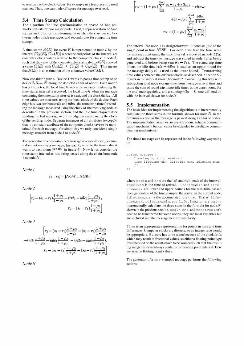
Now consider figure 4. Device 1 wants to pass a time stamp on to

device £ " " " &

along the depicted chain of nodes. Each node

has 3 attributes, the local time when the message containing the

time stamp interval is received, the local time ¥ when the message

containing the time stamp interval is sent, and the clock drift¢

. All

time values are measured using the local clock of the device. Each

edge has two attributes

and

¦ & (

, the round trip time for send-

ing the message measured using the clock of the receiving node as

described in the previous section, and the idle time elapsed after

sending the last message over this edge measured using the clock

of the sending node. Separate instances of all attributes (except¢

that is a constant attribute of the computer clock) have to be main-

tained for each message, for simplicity we only consider a single

message transfer from node 1 to node&

.

The generator of a time–stamped message is a special case, because

it does not receive a message. Instead,

¡

is set to the time value it

wants to pass along (& ¦ ¨

in figure 4). Now let us consider the

time stamp interval as it is being passed along the chain from node

1 to node&

.

Node 1

¦

¡

¡

§

¦

& ¦ ¨ & ¦ ¨§

Node 2

¦

¤

§ ¥

¡

¤

¡

©

£

' ¢

¦

£ ¤

¢

¡

¤

§

¡

¤

¦ & (

¡

£ ¤

¢

¦

£

' ¢

¡

©

¦

¤

§ ¥

¡

¤

¡ ©

£ ¤

¢

¦

£

' ¢

¡

Node 3

¢

¤

§ ¥

¡

¤

¡

©

£

' ¢

¢

£ ¤

¢

¡

¤

§ ¥

¦

¤

¦

©

£

' ¢

¢

£ ¤

¢

¦

¤

§

¡

£

' ¢

¢

£ ¤

¢

¦

¤

¦ & (

¡

£ ¤

¢

¢

£

' ¢

¡

©

¤

§

¦

¤

¦ & (

¦

£ ¤

¢

¢

£

' ¢

¦

©

¢

¤

§ ¥

¡

¤

¡ ©

£ ¤

¢

¢

£

' ¢

¡

¤

§ ¥

¦

¤

¦ ©

£ ¤

¢

¢

£

' ¢

¦

Node N

¤

§

£

' ¢

©

¡

¡

¥

¤

'

¡

£ ¤

¢

¤

¡

' §

£ ¤

¢

©

¡

¡

¦ & (

£

' ¢

¤

§

£ ¤

¢

©

¡

¡

¥

¤

£

' ¢ "

The interval for node 1 is straightforward, it consists just of the

single point in time& ¦ ¨

. For node 2 we take the time when

the message containing the time interval is received in node 2 (

¦

)

and subtract the time the message was stored in node 1 after being

generated and before being sent (¥

¡

¤

¡

). The round trip time

minus the idle time

¡

¤

¦ & (

¡

is used as an upper bound for

the message delay (0 is used as the lower bound). Transforming

time values between the different clocks as described in section 5.2

results in the interval shown for node 2. Continuing this way with

subtracting total node storage time from message arrival time and

using the sum of round trip minus idle times as the upper bound for

the total message delay, and assuming

0

©

, one will end up

with the interval shown for node&

.

5.5 ImplementationThe basic idea for implementing the algorithm is to incrementally

calculate the three sums in the formula shown for node&

in the

previous section as the message is passed along a chain of nodes.

The implementation assumes an asynchronous, reliable communi-cation mechanism but can easily be extended to unreliable commu-

nication mechanisms.

The timed message can be represented in the following way using

C:

struct Message {

Time begin, end, received;

Time lifetime_min, lifetime_max, idletime_min;

/* ... */

};

where begin and end are the left and right ends of the interval,received is the time of arrival, lifetime min and life-

time max are lower and upper bounds for the real–time passed

from generation of the time stamp to the arrival in the current node,

idletime min is the accumulated idle time. That is, life-

time max, idletime min, and lifetime min are used to

incrementally calculate the three sums in the formula for node&

shown in the previous section. begin, end, and received don’t

need to be transferred between nodes, they are local variables but

are included into the message here for simplicity.

Time is an appropriate representation for points in time and time

differences. Computer clocks are discrete, so an integer type would

be appropriate. But care has to be taken because of the clock drift,

which may result in fractional values, so either a floating point type

must be used or the results have to be rounded such that the result-ing integer interval always contains the floating point interval. Here

we assume floating point values.

The generator of a time–stamped message performs the following

actions:



rtt1

rtt2

1 2 3 N

ρ 2 ρ 3 ρΝρ 1

1r = NOW

1s

2

2

r

s

3

3

r

s

N

N

r

s

idle1

idle2

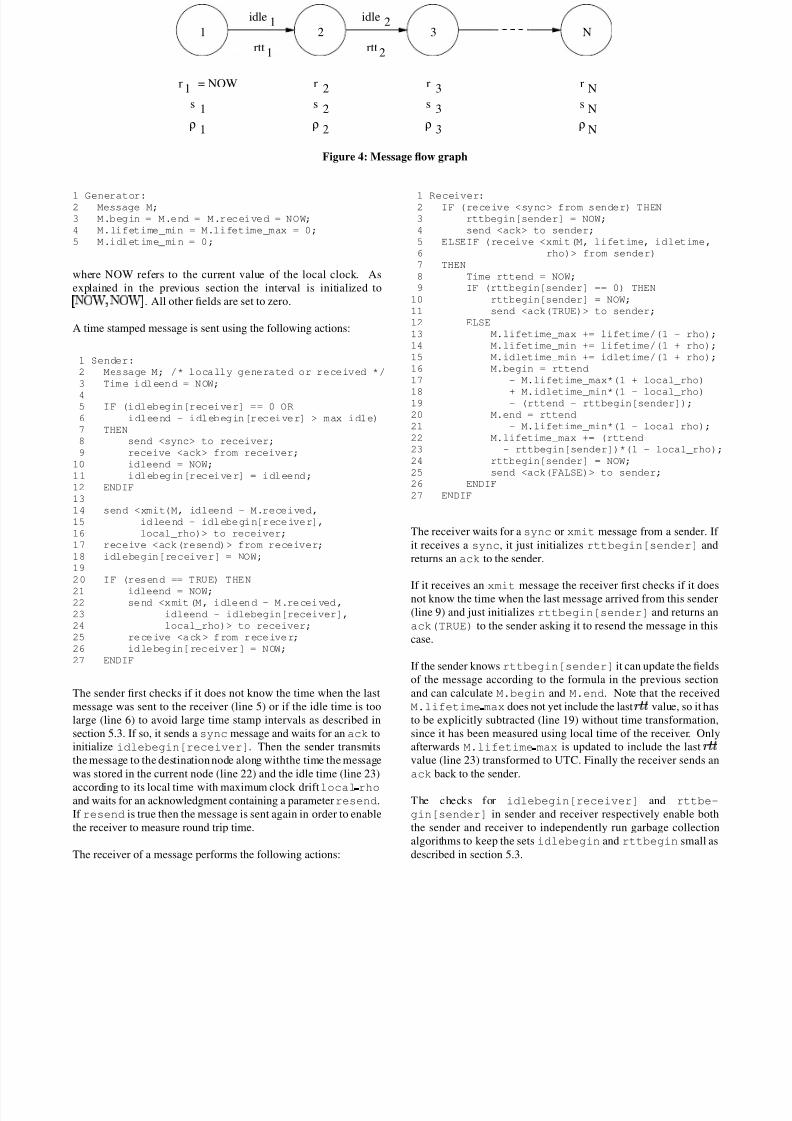
Figure 4: Message flow graph

1 Generator:2 Message M;

3 M.begin = M.end = M.received = NOW;

4 M.lifetime_min = M.lifetime_max = 0;

5 M.idletime_min = 0;

where NOW refers to the current value of the local clock. As

explained in the previous section the interval is initialized to

¦ ¡ £

¢ ¡ £

§

. All other fields are set to zero.

A time stamped message is sent using the following actions:

1 Sender:

2 Message M; /* locally generated or received */

3 Tim e i dl een d = N OW;

45 IF (idlebegin[receiver] == 0 OR

6 idleend - idlebegin[receiver] > max_idle)

7 THEN

8 send <sync> to receiver;

9 receive <ack> from receiver;

10 idleend = NOW;

11 idlebegin[receiver] = idleend;

12 ENDIF

13

14 send <xmit(M, idleend - M.received,

15 id lee nd - idl ebe gi n[r ece ive r],

16 local_rho)> to receiver;

17 receive <ack(resend)> from receiver;

18 idlebegin[receiver] = NOW;

19

20 IF (resend == TRUE) THEN

21 idleend = NOW;22 se nd <x mit (M , i dle en d - M .re cei ved ,

23 idleend - idlebegin[receiver],

24 local_rho)> to receiver;

25 re ce ive <a ck > f rom r ece ive r;

26 id le beg in[ rec eiv er ] = N OW;

27 ENDIF

The sender first checks if it does not know the time when the last

message was sent to the receiver (line 5) or if the idle time is too

large (line 6) to avoid large time stamp intervals as described in

section 5.3. If so, it sends a sync message and waits for an ack to

initialize idlebegin[receiver]. Then the sender transmits

the message to the destination node along withthe time the message

was stored in the current node (line 22) and the idle time (line 23)

according to its local time with maximum clock drift local rhoand waits for an acknowledgment containing a parameter resend.

If resend is true then the message is sent again in order to enable

the receiver to measure round trip time.

The receiver of a message performs the following actions:

1 Receiver:2 IF (receive <sync> from sender) THEN

3 rttbegin[sender] = NOW;

4 send <ack> to sender;

5 ELSEIF (receive <xmit(M, lifetime, idletime,

6 rho)> from sender)

7 THEN

8 Time rttend = NOW;

9 IF (rttbegin[sender] == 0) THEN


11 send <ack(TRUE)> to sender;

12 ELSE

13 M.lifetime_max += lifetime/(1 - rho);

14 M.lifetime_min += lifetime/(1 + rho);

15 M.idletime_min += idletime/(1 + rho);

16 M.begin = rttend

17 - M.lifetime_max*(1 + local_rho)

18 + M.idletime_min*(1 - local_rho)19 - (rttend - rttbegin[sender]);

20 M.end = rttend

21 - M.lifetime_min*(1 - local_rho);

22 M.lifetime_max += (rttend

23 - rttbegin[sender])*(1 - local_rho);


25 send <ack(FALSE)> to sender;

26 ENDIF

27 ENDIF

The receiver waits for a sync or xmit message from a sender. If

it receives a sync, it just initializes rttbegin[sender] and

returns an ack to the sender.

If it receives an xmit message the receiver first checks if it doesnot know the time when the last message arrived from this sender

(line 9) and just initializes rttbegin[sender] and returns an

ack(TRUE) to the sender asking it to resend the message in this

case.

If the sender knows rttbegin[sender] it can update the fields

of the message according to the formula in the previous section

and can calculate M.begin and M.end. Note that the received

M.lifetime max does not yet include the last

value, so it has

to be explicitly subtracted (line 19) without time transformation,

since it has been measured using local time of the receiver. Only

afterwards M.lifetime max is updated to include the last

value (line 23) transformed to UTC. Finally the receiver sends an

ack back to the sender.

The checks for idlebegin[receiver] and rttbe-

gin[sender] in sender and receiver respectively enable both

the sender and receiver to independently run garbage collection

algorithms to keep the sets idlebegin and rttbegin small as

described in section 5.3.



0 100 200 300 400 500 600 700 800 9000

500

1000

1500

2000

2500

3000

3500

4000

Age [s]

I n t e r v a l l e n g t h

[ u s ]

0 1 2 3 4 5 6 70

200

400

600

800

1000

1200

1400

Number of hops

I n t e r v a l l e n g t h

[ u s ]

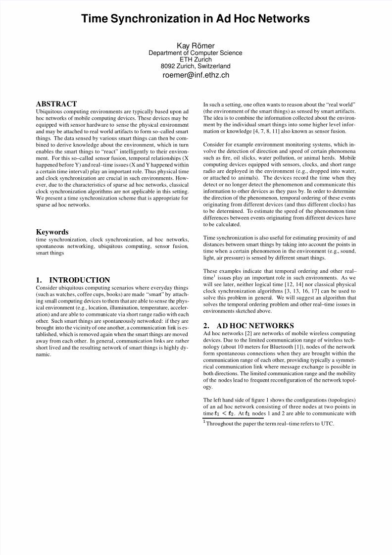
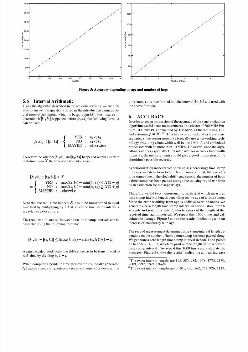
Figure 5: Accuracy depending on age and number of hops

5.6 Interval ArithmeticUsing the algorithm described in the previous sections, we are now

able to answer the questions posed in the introduction using a spe-

cial interval arithmetic, which is based upon [5]. For instance to

determine if ¦

¡

¦

§

happened before ¦

¢ ¥ §

the following formula

can be used:

¦

¡ ¦ § £

¦

¢

¥ §

¡ ¢ £ ¤ ¦ ¨

¦

£

¢

¡

¨

¥£

¡

£ ¤ ¨ ! # % ' ) !

To determine whether ¦

¡ ¦

§

and ¦

¢ ¥ §

happened within a certain

real–time span1

the following formula is used:

2

¦

¡ ¦ §

¤

¦

¢ ¥§

2

£

1

¡ ¢£ ¤ ¦ ¨ 4 6 8

§

¥

¦

©

¤

4 ' @§

¢

¡

© £

1 §

£ ¤

¢

©

¡

¨ 4 6 8§

¢ ¡ ©

¤

4 ' @§

¥ ¦ © A

1 §

£

' ¢

©

£ ¤ ¨ ! # % ' ) !

Note that the real–time interval 1 has to be transformed to local

time first by multiplying by£ E

¢, since the time stamp intervals

are relative to local time.

The real–time “distance” between two time stamp intervals can be

estimated using the following formula:

2

¦

¡ ¦ §

¤

¦

¢ ¥§

2

¡

§4 6 8

§

¥ ¦ ©

¤

4 ' @§

¢ ¡ © © G

§

£ ¤

¢

©

Again the calculated local time difference has to be transformed to

real–time by dividing by£ ¤

¢ .

When comparing points in time (for example a locally generated (

) against time stamp intervals received from other devices, the

time stamp (

is transformed into the interval ¦

( (§

and used with

the above formulas.

6. ACCURACY

In order to get an impression of the accuracy of the synchronizationalgorithm we did some measurements on a cluster of 800 MHz Pen-

tium III Linux PCs connected by 100 Mbit/s Ethernet using TCP

and assuming ¢

£ ©

. This has to be considered as a best case

scenario, since sensor networks typically use a networking tech-

nology providing a bandwidth well below 1 Mbit/s and embedded

processors with no more than 10 MIPS. However, since the algo-

rithm is neither especially CPU intensive nor network bandwidth

intensive, the measurements should give a good impression of the

algorithm’s possible accuracy.

Synchronization inaccuracies show up as (increasing) time stamp

intervals and stem from two different sources: first, the age of a

time stamp (due to the clock drift), and second, the number of hops

a time stamp has been passed along (due to using round trip time

as an estimation for message delay).

Therefore we did two measurements, the first of which measures

time stamp interval length depending on the age of a time stamp.

Since the error resulting from age is additive over the nodes, we

generate a zero length time stamp interval in node 1, store it for X

seconds and send it to node 2, which prints out the length of the

received time stamp interval. We repeat this 1000 times and cal-

culate the average. Figure 5 shows the results2, indicating a linear

increase of inaccuracy with age.

The second measurement determines time stamp interval length de-

pending on the number of hops a time stamp has been passed along.

We generate a zero length time stamp interval in node 1 and pass it

on to node 2, 3, ..., 7, which all print out the length of the received

time stamp interval. We repeat this 1000 times and calculate the

averages. Figure 5 shows the results3, indicating a linear increase¦

The exact interval lengths are 195, 585, 982, 1378, 1775, 2170,2609, 2992, 3369, 3764 H s.¢

The exact interval lengths are 0, 201, 400, 562, 752, 926, 1113,



of inaccuracy with the number of hops.

Since the two types of inaccuracies are additive one can interpret

the measurements as follows: Passing a time stamp along no more

than 5 hops with an age of no more than 500 seconds one can ex-

pect an inaccuracy of no more than 3ms in the examined setting,

which is a reasonable value compared to existing clock synchro-

nization algorithms. What this means is that the algorithm will be

able to give an exact answer (as opposed to MAYBE) when com-

paring time stamps representing points in time with more than 6ms

in between, since then the resulting time stamp intervals (3ms each)

cannot overlap. With less than 6ms in between the algorithm might

still give an exact answer, but MAYBE answers are likely.

7. IMPROVEMENTSThere are several ways to improve the accuracy of the algorithm

(i.e., reduce the probability of MAYBE results), which are worth

further investigation.

One idea to avoid MAYBE results when comparing time stamps

originating from the same node is to keep a history of time stamps

instead of only one time stamp. Instead of updating the single time

stamp upon receipt, the receiving node appends the updated time

stamp together with a unique node identification

and its¢

value

to the time stamp history or reuses a time stamp from the history if

there already is an entry for this node in the history. If comparing

time stamps results in MAYBE then the histories of the compared

stamps are searched for common nodes and the comparison is re-peated using the time stamps of these common nodes, transforming

time values if necessary, using the ¢ values stored in the history.

This is likely to give a “better” answer, since inaccuracy increases

with age and hop count of the time stamps. For the same reason the

accuracy of calculated real–time spans can be improved by using

“younger” time stamps from the history in the same way whenever

possible.

A different and more general idea is to replace MAYBE results

with a probability depending on the layout of the compared time

stamp intervals, i.e., the algorithm would then answer 1

£

with

probability ¢ instead of 1 £ ¥ § ©(

£

. To implement this we

have to find out probability distributions for the time instants over

the time stamp intervals.

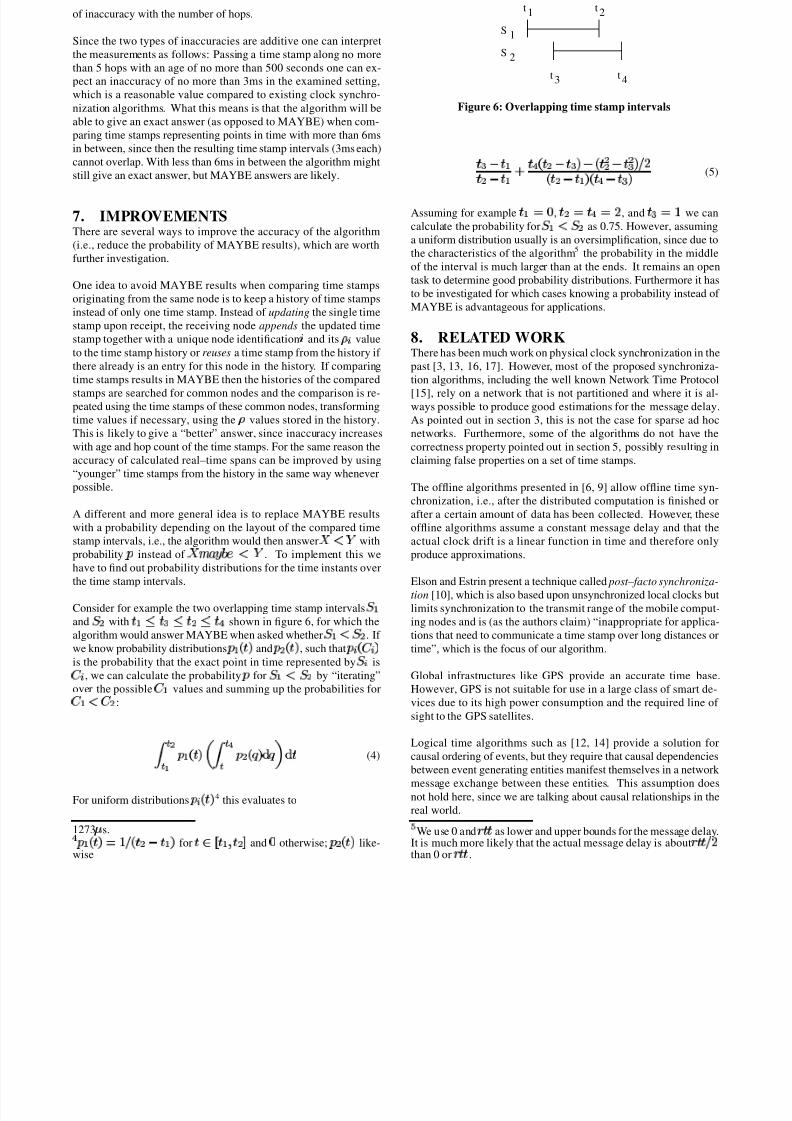
Consider for example the two overlapping time stamp intervals2

¡

and2

¦

with ¡

¡

¢

¡

¦

¡

¥

shown in figure 6, for which the

algorithm would answer MAYBE when asked whether2

¡

£

2

¦

. If

we know probability distributions¢

¡

§

©

and¢

¦

§

©

, such that¢

§ ¦

©

is the probability that the exact point in time represented by 2 is

¦ , we can calculate the probability

¢for

2

¡ £

2

¦

by “iterating”

over the possible ¦

¡

values and summing up the probabilities for

¦

¡

£

¦

¦

:

¢

¡

§

©

¢

¦

§

© %

%

(4)

For uniform distributions ¢ §

© 4 this evaluates to

1273H

s.¥

¢

¡

§

©

£

G

§

§ ¦

¤

¡ ©

for

¦

¡ ¦ §

and©

otherwise;¢

¦

§

©

like-wise

S

S

t1

t2

1

2

t t3 4

Figure 6: Overlapping time stamp intervals

¢

¤

¡

¦

¤

¡

'

¥

§

¦

¤

¢©

¤

§

¦

¦

¤

¦

¢

© G

§

¦

¤

¡

©

§

¥

¤

¢©

(5)

Assuming for example

¡

©

,

¦

¥

, and

¢

£

we can

calculate the probability for 2

¡

£

2

¦

as 0.75. However, assuming

a uniform distribution usually is an oversimplification, since due to

the characteristics of the algorithm5 the probability in the middle

of the interval is much larger than at the ends. It remains an open

task to determine good probability distributions. Furthermore it has

to be investigated for which cases knowing a probability instead of

MAYBE is advantageous for applications.

8. RELATED WORKThere has been much work on physical clock synchronization in the

past [3, 13, 16, 17]. However, most of the proposed synchroniza-

tion algorithms, including the well known Network Time Protocol

[15], rely on a network that is not partitioned and where it is al-ways possible to produce good estimations for the message delay.

As pointed out in section 3, this is not the case for sparse ad hoc

networks. Furthermore, some of the algorithms do not have the

correctness property pointed out in section 5, possibly resulting in

claiming false properties on a set of time stamps.

The offline algorithms presented in [6, 9] allow offline time syn-

chronization, i.e., after the distributed computation is finished or

after a certain amount of data has been collected. However, these

offline algorithms assume a constant message delay and that the

actual clock drift is a linear function in time and therefore only

produce approximations.

Elson and Estrin present a technique called post–facto synchroniza-

tion [10], which is also based upon unsynchronized local clocks but

limits synchronization to the transmit range of the mobile comput-

ing nodes and is (as the authors claim) “inappropriate for applica-

tions that need to communicate a time stamp over long distances or

time”, which is the focus of our algorithm.

Global infrastructures like GPS provide an accurate time base.

However, GPS is not suitable for use in a large class of smart de-

vices due to its high power consumption and the required line of

sight to the GPS satellites.

Logical time algorithms such as [12, 14] provide a solution for

causal ordering of events, but they require that causal dependencies

between event generating entities manifest themselves in a network

message exchange between these entities. This assumption doesnot hold here, since we are talking about causal relationships in the

real world.

We use 0 and

as lower and upper bounds for the message delay.It is much more likely that the actual message delay is about

G

than 0 or

.



9. CONCLUSION AND OUTLOOKWe pointed out the problem of physical time synchronization in

sparse ad hoc networks giving two reasons why classical clock syn-

chronization algorithms fail in this environment.

We then presented a synchronization algorithm suitable for a cer-

tain class of applications of sparse ad hoc networks, which trans-

forms time stamps exchanged between nodes inside messages to

the local time of the receiver instead of adjusting the clocks. The

algorithm has a low resource and message overhead and therefore

is well suited for resource restricted distributed sensor networks.

There are several prototype implementations of the algorithm. We

are currently working on an event distribution service with tem-

poral delivery order of time stamped events for ad hoc networks,

which is based on the presented algorithm. We intend to use

this service for time dependent sensor fusion in the Smart–Its

project[4].

Further research will focus on working out the improvements

sketched in section 7. Another interesting point is how to select the

initial time stamp interval that represents the point in time when an

external event has been sensed. In the description of the algorithm

we assumed that the event we want to time stamp happens “inside”

the computing device and therefore we started with a zero length

interval ¦

& ¦ ¨ & ¦ ¨§

. However, often a “real world” event is

sensed by an external sensor, which itself is connected to the com-

puting device. Furthermore, the detection of the event in the com-

puting device might be indeterministically delayed due to software.In such cases one should already start with a non–zero time inter-

val that contains the point in time the event was sensed. There is

no obvious way to determine this interval except calculating it from

the properties of the technology that is used. Last but not least, we

will have to examine and evaluate different strategies for handling

connections to large numbers of peers as pointed out at the end of

section 5.3.

10. REFERENCES[1] Bluetooth SIG. www.bluetooth.org.

[2] MANET IETF working group.

www.ietf.org/html.charters/manet-charter.html.

[3] Network Time Synchronization Bibliography.www.eecis.udel.edu/ mills/bib.htm.

[4] Smart-Its Project. www.smart-its.org.

[5] J. F. Allen. Maintaining Knowledge about Temporal

Intervals. Communications of the ACM , 26(11):832–843,

November 1983.

[6] P. Ashton. Algorithms for off-line clock synchronization.

Technical Report TR COSC 12/95, Department of Computer

Science, University of Canterbury, December 1995.

[7] M. Beigl, H.W. Gellersen, and A. Schmidt. MediaCups:

Experience with Design and Use of Computer-Augmented

Everyday Objects. Computer Networks, Special Issue on

Pervasive Computing, 25(4):401–409, March 2001.

[8] A. Cerpa, J. Elson, D. Estrin, L. Girod, M. Hamilton, and

J. Zhao. Habitat Monitoring: Application Driver for Wireless

Communications Technology. In 2001 ACM SIGCOMM

Workshop on Data Communications in Latin America and

the Caribbean, San Jose, Costa Rica, April 2001.

[9] A. Duda, G. Harrus, Y. Haddad, and G. Bernard. Estimating

global time in distributed systems. In 7th International

Conference on Distributed Computing Systems (ICDCS’87),

Berlin, Germany, September 1987. IEEE.

[10] J. Elson and D. Estrin. Time Synchronization for Wireless

Sensor Networks. In 2001 International Parallel and

Distributed Processing Symposium (IPDPS), Workshop on

Parallel and Distributed Computing Issues in Wireless

Networks and Mobile Computing, San Francisco, USA, April

2001.

[11] S. Hollar. COTS Dust. Masters thesis, University of

California, Berkeley, 2000.

[12] L. Lamport. Time, Clocks, and the Ordering of Events in a

Distributed System. Communications of the ACM ,

21(4):558–565, July 1978.

[13] L. Lamport and P. M. Melliar-Smith. Synchronizing Clocks

in the Presence of Faults. Journal of the ACM , 32(1), January

1985.

[14] F. Mattern. Virtual Time and Global States in Distributed

Systems. In Workshop on Parallel and Distributed

Algorithms, Chateau de Bonas, October 1988.

[15] D. L. Mills. Improved algorithms for synchronizing

computer network clocks. In Conference on Communication

Architectures (ACM SIGCOMM’94), London, UK, August

1994. ACM.

[16] P. Ramanathan, K. G. Shin, and R. W. Butler. Fault-Tolerant

Clock Synchronization in Distributed Systems. In C. J.

Walter, M. M. Hugue, and Neeraj Suri, editors, Advances in

Ultra-Dependable Distributed Systems. IEEE Computer

Society, Los Alamitos, USA, January 1995.

[17] B. Simons, J. Welch, and N. Lynch. An overview of clock

synchronization. Technical Report RJ 6505, IBM Almaden

Research Center, 1988.

Documents

Ad Hoc Synchronization