Embed Size (px)
Citation preview

Algorithms for the computation and inversion ofcumulative gamma distributions
Javier Segura
Departamento de Matemáticas, Estadística y Computación.Universidad de Cantabria, Spain
In collaboration with Amparo Gil and Nico M. Temme.
J. Segura (Universidad de Cantabria) Gamma and χ2 distributions SCINUM ’14, Vienna 1 / 27

Introduction and definitions
Cumulative γ and χ2 distributions
The cumulative central gamma distribution is given by the incomplete gammafunction ratios
Pµ(y) =γ(µ, x)
Γ(µ)=
1Γ(µ)
∫ y
0tµ−1e−tdt ,
The non-central γ distribution can be defined as
Pµ(x , y) = e−x∞∑
n=0
xn
n!Pµ+n(y),
From the Maclaurin series for modified Bessel functions Iµ(z) we obtain:
Pµ(x , y) = x12 (1−µ)
∫ y
0t
12 (µ−1)e−t−x Iµ−1
(2√
xt)
dt .
Observe that Pµ(0, y) = 0, Pµ(0,+∞) = 1.Pµ(0, y) = Pµ(y).
J. Segura (Universidad de Cantabria) Gamma and χ2 distributions SCINUM ’14, Vienna 2 / 27

Introduction and definitions
The complementary distributions are obtained by changing the interval ofintegration from [0, y ], to [y ,+∞). We have
Qµ(x , y) = x12 (1−µ)
∫ +∞
yt
12 (µ−1)e−t−x Iµ−1
(2√
xt)
andPµ(x , y) + Qµ(x , y) = 1.
The Q-function is also called generalized Marcum Q-function.
Similarly as before,
Qµ(y) =Γ(µ, y)
Γ(µ)=
1Γ(µ)
∫ +∞
ytµ−1e−tdt
and
Qµ(x , y) = e−x∞∑
n=0
xn
n!Qµ+n(y).
J. Segura (Universidad de Cantabria) Gamma and χ2 distributions SCINUM ’14, Vienna 3 / 27

Introduction and definitions
Pµ(x , y) is a cumulative distrubition function (CDF) with probability densityfunction (PDF)
fµ(x , t) =1
Γ(µ)x
12 (1−µ)t
12 (µ−1)e−t−x Iµ−1
(2√
xt),
that is,
Pµ(x , y) =
∫ y
0fµ(x , t)dt
For a fixed values of x , µ and p, denote as Fµ(x ,p) the inverse with respectto y :
Pµ(x ,Fµ(x ,p)) = p.
Random number generation:
If U is a random uniform variable in [0,1] then Y = Fµ(x ,U) is a randomvariable with PDF as before.A different way to generate random samples with a given PDF isacceptance-rejection method (the CDF is needed in this case)
J. Segura (Universidad de Cantabria) Gamma and χ2 distributions SCINUM ’14, Vienna 4 / 27

Introduction and definitions
An analysis of the situation revealed that:
1 Algorithms existed both for the computation and inversion (with respectto y ) of the CDF for the central case, but that asymptotics could improveboth algorithms.
2 No algorithms were available for the computation of the CDFs for thenoncentral case for real µ, and the available software had a limited rangeof validity (and also some inaccuracies, as we will see).
3 Algorithms for the inversion in the noncentral case also had a limitedrange of validity (the inversion with respect to x is also important inapplications). No published software was available.
J. Segura (Universidad de Cantabria) Gamma and χ2 distributions SCINUM ’14, Vienna 5 / 27

Computation and inversion in the central case Computation of the central distribution
Computation of the central distribution
Recall the definitions
Pa(y) =1
Γ(a)
∫ y
0ta−1e−tdt ,Qa(y) =
1Γ(a)
∫ +∞
yta−1e−tdt
Because Pa(y) + Qa(y) = 1 we only need to compute one function. Wecompute the smallest of the two.
For large values of a, x we have a transition at a ∼ x , with
Pa(y) . 12 when a & y ,
Qa(y) . 12 when a . y .
J. Segura (Universidad de Cantabria) Gamma and χ2 distributions SCINUM ’14, Vienna 6 / 27

Computation and inversion in the central case Computation of the central distribution
Accordingly, the methods of computation are divided in two zones, withseveral methods of computation in each one.
10
20
30
40
50
10 20 30 40 50
x = 0.3 a
x = 2.35 a
a
x
a = α(x)
a = 12
1.5
UA
CF
PT
QT
PT: Taylor series for P.QT: Taylor series for Q (small triangle).UA: Uniform asymptotic expansions.CF: continued fraction for the Q.
J. Segura (Universidad de Cantabria) Gamma and χ2 distributions SCINUM ’14, Vienna 7 / 27

Computation and inversion in the central case Inversion of the central distribution
Inversion of the central distribution
As commented, the inversion is also needed in applications.For fixed a, we invert Pa(y) = p or, equivalently, Qa(y) = q.
Our approach:
1 Invert Pa(y) (Qa(y)) if p < q (p > q)2 Use the existent approximation methods (PT, Poincaré asymptotics for
Q, UA) to find starting values.3 Apply higher order Newton methods from the resulting starting values.
The different type of starting values are chosen according to the next figure.
J. Segura (Universidad de Cantabria) Gamma and χ2 distributions SCINUM ’14, Vienna 8 / 27

Computation and inversion in the central case Inversion of the central distribution
Starting values (an example):For small p, we use PT to write
x = r +∞∑
n=2
ck r k ,
where r = (pΓ(1 + a))1/a and by expanding, the first few coefficients are
c2 =1
a + 1,
c3 =3a + 5
2(a + 1)2(a + 2),
c4 =8a2 + 33a + 31
3(a + 1)3(a + 2)(a + 3),
c5 =125a4 + 1179a3 + 3971a2 + 5661a + 2888
24(1 + a)4(a + 2)2(a + 3)(a + 4).
J. Segura (Universidad de Cantabria) Gamma and χ2 distributions SCINUM ’14, Vienna 9 / 27

Computation and inversion in the central case Inversion of the central distribution
The accuracy of the starting values is shown in this figure
020
4060
80100
0
50
100
1500
1
2
3
4
5
x 10−3
xa
dr(x
,xin
i)
2-3 iterations (in the worst cases) with a fourth order Newton method give arel. accuracy ∼ 10−13
A. Gil, J. Segura, N.M. Temme. SIAM J Sci Comput 34(6) (2012) A2965-A2981.
W. Gautschi. ACM Trans. Math. Software 5 (1979) 466–481.
A. R. DiDonato, A. H. Morris. ACM Trans. Math. Software 12 (1986) 377–393.
J. Segura (Universidad de Cantabria) Gamma and χ2 distributions SCINUM ’14, Vienna 10 / 27

Computation and inversion of the noncentral distribution Computation of the non-central distribution
Computation of the non-central distributionThe generalized Marcum Q-function is the non-central cumulative χ2
distribution, up to elementary redefinition of the variables. We recall that
Qµ(x , y) = x12 (1−µ)
∫ +∞
yt
12 (µ−1)e−t−x Iµ−1
(2√
xt)
dt ,
where µ > 0 and Iµ(z) is the modified Bessel function.
The complementary function such that Pµ(x , y) + Qµ(x , y) = 1 :
Pµ(x , y) = x12 (1−µ)
∫ y
0t
12 (µ−1)e−t−x Iµ−1
(2√
xt)
dt .
Particular values are
Qµ(x ,0) = 1, Qµ(x ,+∞) = 0,
Qµ(0, y) = Qµ(y), Qµ(+∞, y) = 1,
Q+∞(x , y) = 1.
J. Segura (Universidad de Cantabria) Gamma and χ2 distributions SCINUM ’14, Vienna 11 / 27

Computation and inversion of the noncentral distribution Computation of the non-central distribution
As for incomplete gamma functions, we compute the smallest of the twofunctions. Asymptotic analysis gives that for large values of µ, x , y , we have atransition at y ∼ x + µ, with
Pµ(x , y) . Qµ(x , y) when y . x + µ,
Qµ(x , y) . Pµ(x , y) when y & x + µ.
Ingredients in the computation:
1 Series in terms of incomplete gamma functions.
2 Recurrence relations.
3 Asymptotic expansions for large µ in terms of the error function (both forP and Q).
4 Asymptotic expansions for large xy .
5 Quadrature methods.
We give some details of these methods.
J. Segura (Universidad de Cantabria) Gamma and χ2 distributions SCINUM ’14, Vienna 12 / 27
Computation and inversion of the noncentral distribution Computation of the non-central distribution
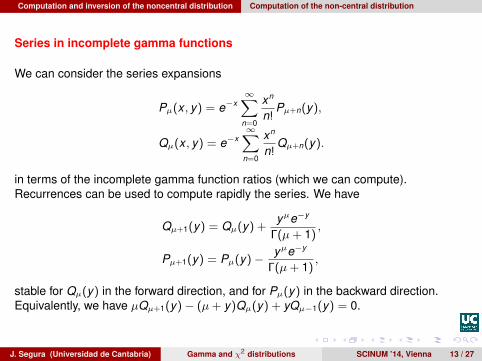
Series in incomplete gamma functions
We can consider the series expansions
Pµ(x , y) = e−x∞∑
n=0
xn
n!Pµ+n(y),
Qµ(x , y) = e−x∞∑
n=0
xn
n!Qµ+n(y).
in terms of the incomplete gamma function ratios (which we can compute).Recurrences can be used to compute rapidly the series. We have
Qµ+1(y) = Qµ(y) +yµe−y
Γ(µ+ 1),
Pµ+1(y) = Pµ(y)− yµe−y
Γ(µ+ 1),
stable for Qµ(y) in the forward direction, and for Pµ(y) in the backward direction.Equivalently, we have µQµ+1(y)− (µ+ y)Qµ(y) + yQµ−1(y) = 0.
J. Segura (Universidad de Cantabria) Gamma and χ2 distributions SCINUM ’14, Vienna 13 / 27

Computation and inversion of the noncentral distribution Computation of the non-central distribution
The series
Qµ(x , y) = e−x∞∑
n=0
xn
n!Qµ+n(y)
can be computed from two values Qµ(y) and Qµ+1(y) and forward recursion with
Qµ+1(y) =
(1 +
yµ
)Qµ(y)− y
µQµ−1(y)
For the other series, we write
Pµ(x , y) ' e−x Pµ(y)
n0∑n=0
xn
n!
Pµ+n(y)
Pµ(y),
estimate the value n0 which gives sufficient accuracy and compute using thebackward recursion
Pµ−1(y) = −µy
Pµ+1(y) +
(1 +
µ
y
)Pµ(y)
J. Segura (Universidad de Cantabria) Gamma and χ2 distributions SCINUM ’14, Vienna 14 / 27

Computation and inversion of the noncentral distribution Computation of the non-central distribution
Recurrence relations
Integration by parts gives the following recurrences
Qµ+1(x , y) = Qµ(x , y) +(y
x
)µ/2e−x−y Iµ(2
√xy),
Pµ+1(x , y) = Pµ(x , y)−(y
x
)µ/2e−x−y Iµ(2
√xy),
It is possible to eliminate the Bessel function and obtain a homogeneous recurrencerelation.
xQµ+2(x , y) = (x − µ)Qµ+1(x , y) + (y + µ)Qµ(x , y)− yQµ−1(x , y),
and Pµ(x , y) satisfies the same relation, but its computation with this recurrence isbadly conditioned (it is subdominant, but not minimal)A better possibility is:
yµ+1 − (1 + cµ)yµ + cµyµ−1 = 0, cµ =
√yx
Iµ (2√
xy)
Iµ−1 (2√
xy).
P is minimal and Q is dominant. Pincherle’s theorem gives:
Pµ(x , y)
Pµ−1(x , y)=
cµ1 + cµ−
cµ+1
1 + cµ+1−. . .
J. Segura (Universidad de Cantabria) Gamma and χ2 distributions SCINUM ’14, Vienna 15 / 27

Computation and inversion of the noncentral distribution Computation of the non-central distribution
Asymptotic expansions for µ large
We start from
Qµ+1(µx , µy) =µe−µx
(2x)µ+1
∫ ∞ξ
ze−µφ(z)e−µη(z)Iµ(µz) dz,
where
φ(z) = − ln z +1
4xz2 − η(z), η(z) =
√1 + z2 + log
z
1 +√
1 + z2, ξ = 2
√xy
The saddle point follows from the equation φ′(z) = 0. It follows that the positivesaddle point z0 is given by
z0 = 2√
x(1 + x). (1)
The transition line in the scaled variables is y = x + 1.
The saddle point coalesces with the end point of integration as y → x + 1. Bleinstein’smethod is a good choice (we omit details).
Q is computed for y > x + 1 (in the unscaled variables y > x + µ).For P analogous expansions can be worked out (y < x + µ)
J. Segura (Universidad de Cantabria) Gamma and χ2 distributions SCINUM ’14, Vienna 16 / 27

Computation and inversion of the noncentral distribution Computation of the non-central distribution
Qµ(µx, µy) ∼ 12 erfc
(−ζ√µ/2
)+
õ
2π
∞∑k=1
Bk − e−12µζ
2e−µη(ξ)Iµ(µξ).
Bk =k∑
j=0
fj,k−j Ψj (ζ)
µk−j
Ψj (ζ) =
( 2
µ
)(j+1)/2 ∫ ∞−ζ√µ/2
e−s2sj ds.
which can be written in terms of incomplete gamma functions.
ζ = sign(x + 1− y)√
2 (φ(ξ)− φ(z0)).
fk (w) =z
2x
uk (t)
(1 + z2)14
dz
dw=∞∑j=0
fjk (w − ζ)j, t = 1/
√1 + z2
φ(z)− φ(ξ) = 12 w2 − ζw, ξ = 2
√xy
u0(t) = 1, u1(t) =3t − 5t3
24, u2(t) =
81t2 − 462t4 + 385t6
1152,
and other coefficients can be obtained by applying the formula
uk+1(t) = 12 t2(1− t2)u′k (t) + 1
8
∫ t
0(1− 5s2)uk (s) ds, k = 0, 1, 2, . . . .
J. Segura (Universidad de Cantabria) Gamma and χ2 distributions SCINUM ’14, Vienna 17 / 27

Computation and inversion of the noncentral distribution Computation of the non-central distribution
Numerical quadrature
We start from the contour integral representation for the function Qµ(x , y)
Qµ(x , y) =e−x−y
2πi
∫LQ
ex/s+ys
1− sdssµ,
where LQ is a vertical line that cuts the real axis in a point s0, with 0 < s0 < 1.Introducing scaled variables x , y and integrating along the path of steepestdescent, we arrive to:
Qµ(µx , µy) =e−
12µζ
2
2π
∫ π
−πe−µψ(θ)f (θ) dθ,
for specific ζ, ψ, f .
The integrand is analytic and vanishing with all derivatives at ±π
The trapezoidal rule is very efficient for this type of integrals.
J. Segura (Universidad de Cantabria) Gamma and χ2 distributions SCINUM ’14, Vienna 18 / 27

Computation and inversion of the noncentral distribution Computation of the non-central distribution
The methods are combined as follows:
Let ξ = 2√
xy and
f1(x , µ) = x + µ−√
4x + 2µ, f2(x , µ) = x + µ+√
4x + 2µ. (2)
Then the scheme is as follows:
1 If x < 30, then compute the series expansion.
2 If ξ > 30 and µ2 < 2ξ, then compute the asymptotic expansion for largeξ.
3 If f1(x , µ) < y < f2(x , µ) and µ < 135, then compute the Marcumfunctions using three-term recurrence relations.
4 If f1(x , µ) < y < f2(x , µ) and µ ≥ 135, then use the asymptotic expansionfor µ large.
5 In other case: compute the integral representation.
J. Segura (Universidad de Cantabria) Gamma and χ2 distributions SCINUM ’14, Vienna 19 / 27

Computation and inversion of the noncentral distribution Computation of the non-central distribution
Our implementation: A. Gil, J. Segura, N.M. Temme, Algorithm 939: Computation ofthe Marcum Q-function ACM Trans. Math. Soft. 40(3) (2014).
An accuracy ∼ 10−12 is obtained in the parameter region(x , y , µ) ∈ [0, A]× [0, A]× [1, A], for A = 200. For larger parameters theaccuracy decreases a little (close to 5 10−11 for A = 105).
Previous work includes:
C.W. Helstrom. IEEE Trans. Inf. Theory (1992)
D.A. Shnidman. IEEE Trans. Inf. Theory (1989)
But no verified public software was available until algorithm 939.
Previously existing software reduces to MATLAB & Mathematica. Are theyreliable?
J. Segura (Universidad de Cantabria) Gamma and χ2 distributions SCINUM ’14, Vienna 20 / 27
Computation and inversion of the noncentral distribution Computation of the non-central distribution
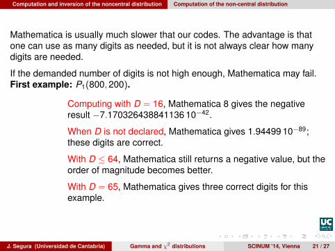
Mathematica is usually much slower that our codes. The advantage is thatone can use as many digits as needed, but it is not always clear how manydigits are needed.
If the demanded number of digits is not high enough, Mathematica may fail.First example: P1(800,200).
Computing with D = 16, Mathematica 8 gives the negativeresult −7.170326438841136 10−42.
When D is not declared, Mathematica gives 1.94499 10−89;these digits are correct.
With D ≤ 64, Mathematica still returns a negative value, but theorder of magnitude becomes better.
With D = 65, Mathematica gives three correct digits for thisexample.
J. Segura (Universidad de Cantabria) Gamma and χ2 distributions SCINUM ’14, Vienna 21 / 27
Computation and inversion of the noncentral distribution Computation of the non-central distribution
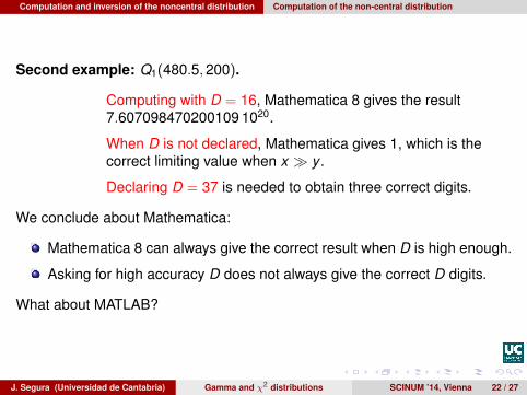
Second example: Q1(480.5,200).
Computing with D = 16, Mathematica 8 gives the result7.607098470200109 1020.
When D is not declared, Mathematica gives 1, which is thecorrect limiting value when x � y .
Declaring D = 37 is needed to obtain three correct digits.
We conclude about Mathematica:
Mathematica 8 can always give the correct result when D is high enough.
Asking for high accuracy D does not always give the correct D digits.
What about MATLAB?
J. Segura (Universidad de Cantabria) Gamma and χ2 distributions SCINUM ’14, Vienna 22 / 27

Computation and inversion of the noncentral distribution Computation of the non-central distribution
MATLAB is based on Shnidman algorithm and has the following limitations:
Only integer values of µ.
Only Marcum Q−function, not P−function.
Slower performances than our algorithms.
Serious errors in MATLAB!
Especially near the transition line y = x + µ.
The plot of the increasing function Q2(x ,200) as a function of x showsvery rapid oscillations for 0 < x < 2400.
The plot of the decreasing function Q800(1, y) as a function of y showsseveral abrupt changes in the interval [750,850], with a steep jump closeto y = 800. Results are meaningless for 800 < y < 1100.
And many more errors were found.
J. Segura (Universidad de Cantabria) Gamma and χ2 distributions SCINUM ’14, Vienna 23 / 27

Computation and inversion of the noncentral distribution Inversion of the noncentral distribution
Inversion of the noncentral distribution
The problem is inverting with respect to x or y the equations
Qµ(x , y) = q, Pµ(x , y) = p.
In statistics,
the inversion of Qµ(x , y) with respect to x corresponds to the problem ofinverting the distribution function with respect to the noncentralityparameter given the upper tail probability.
The inversion of Pµ(x , y) with respect to y with fixed x corresponds tothe problem of computing the p-quantiles of the distribution function.This is related to the generation of random numbers corresponding to anoncentral gamma distribution
J. Segura (Universidad de Cantabria) Gamma and χ2 distributions SCINUM ’14, Vienna 24 / 27
Computation and inversion of the noncentral distribution Inversion of the noncentral distribution
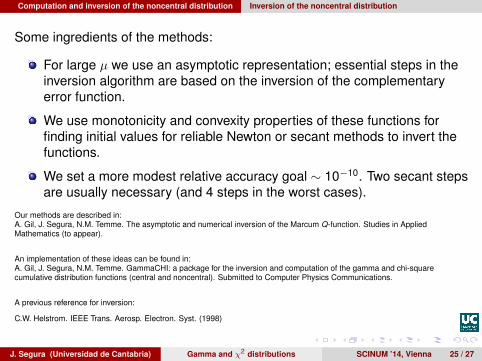
Some ingredients of the methods:
For large µ we use an asymptotic representation; essential steps in theinversion algorithm are based on the inversion of the complementaryerror function.
We use monotonicity and convexity properties of these functions forfinding initial values for reliable Newton or secant methods to invert thefunctions.
We set a more modest relative accuracy goal ∼ 10−10. Two secant stepsare usually necessary (and 4 steps in the worst cases).
Our methods are described in:A. Gil, J. Segura, N.M. Temme. The asymptotic and numerical inversion of the Marcum Q-function. Studies in AppliedMathematics (to appear).
An implementation of these ideas can be found in:A. Gil, J. Segura, N.M. Temme. GammaCHI: a package for the inversion and computation of the gamma and chi-squarecumulative distribution functions (central and noncentral). Submitted to Computer Physics Communications.
A previous reference for inversion:
C.W. Helstrom. IEEE Trans. Aerosp. Electron. Syst. (1998)
J. Segura (Universidad de Cantabria) Gamma and χ2 distributions SCINUM ’14, Vienna 25 / 27

Next steps
Next steps:1 About direct computation: should we consider a generalization of
Marcum-Q? The Nuttal Q-function:
Qη,µ(x , y) = x12 (1−µ)
∫ +∞
ytη+ 1
2 (µ−1)e−t−x Iµ−1
(2√
xt)
dt ,
Q0,µ(x , y) = Qµ(x , y)
2 Other important cumulative distribution functions: the betadistribution function.
J. Segura (Universidad de Cantabria) Gamma and χ2 distributions SCINUM ’14, Vienna 26 / 27

Thank you
Thank you!
J. Segura (Universidad de Cantabria) Gamma and χ2 distributions SCINUM ’14, Vienna 27 / 27


![Title Fault-Tolerant Quantum Computation on Logical Cluster ......quantum computation under imperfect gate operations, namely fault-tolerant quantum computation [11, 12]. The main](https://img.pdfslide.tips/doc/110x75/60f3fd58ff2b1f2547000d7a/title-fault-tolerant-quantum-computation-on-logical-cluster-quantum-computation.jpg)