Embed Size (px)
Citation preview

國 立 交 通 大 學
電控工程研究所
碩士論文
無線感測網路錨節點之反向定位法
An Approach to Reversely Locating Anchor Nodes in Wireless
Sensor Network
研 究 生:李勇叡
Student: Yung-Jui Lee
指導教授:黃育綸 博士
Advisor: Dr. Yu-Lun Huang
中華民國一百零一年四月
4, 2012

無線感測網路錨節點之反向定位法
An Approach to Reversely Locating Anchor Nodes in Wireless Sensor
Network
研 究 生:李勇叡 Student: Yung-Jui Lee
指導教授:黃育綸 博士 Advisor: Dr. Yu-Lun Huang
國 立 交 通 大 學
電控工程研究所
碩士論文
A Thesis
Submitted to Institute of Electrical Control Engineering
College of Electrical Engineering
National Chiao Tung University
in partial Fulfill of the Requirements
for the Degree of
Master
in
Institute of Electrical Control Engineering
4, 2012
Hsinchu, Taiwan, Republic of China
中華民國一百零一年四月

無無無線線線感感感測測測網網網路路路錨錨錨節節節點點點之之之反反反向向向定定定位位位法法法
學生:李勇叡 指導教授:黃育綸 博士
國 立 交 通 大 學 電控工程研究所(研究所)碩士班
摘摘摘 要要要
無線感測網路定位已經成為各種新穎應用(如土石流偵測、精緻農業、健康照護等)高
度需求的功能之一。透過錨節點(anchor node)的參考位置值及與感測節點(sensor node)
之間的訊號強度,即可定位無線感測網路中的感測節點。在這類設計中,錨節點的位置愈精
確,感測節點的定位結果就會愈正確。 為了要提供精確的錨節點位置資訊,許多研究利用
GPS裝置來定位戶外的無線感測網路中的感測節點。由於 GPS裝置無法在室內環境中得到精
確的位置資訊,因此,有部分定位方法會利用手動設定錨節點位置的方式來得到較精確的感測
節點位置。然而,手動設定錨節點的方法卻無法應用於大型無線感測網路中,而且,手動設定
的人工錯誤也可能會逐漸累積,並影響無線感測網路的定位結果。在這篇論文中,我們研究
多種反向定位802.11無線網路存取點的方法。有些方法仍舊採用GPS模組來定位錨節點(存取
點)的位置;有一些則嚴格地限制訓練階段的條件(固定的啟始點與行進方向)。 為了改善
這些問題與限制,我們提出一種新的無線感測網路反向定位錨節點的方法。我們的方法不需
要GPS模組,也不需要嚴格的訓練限制。考慮到無線通訊晶片的個體差異,在我們開始進入
訓練階段之前,我們先對無線感測節點進行校正,以取得評估節點距離所需的 RSSI 係數,以
利反向定位錨節點。我們利用 MSP430FS5438/CC2500EMK實驗板進行多種實驗,以便於
精確性與成本之間取得平衡。我們同時也說明如何應用我們的方法來估測錨節點位置,並將
估測的位置應用於現有的定位方法中,以利定位感測節點。實驗結果顯示:1)如果先進行校
正或移除訓練限制,我們就可以得到較高的精確度; 2)比起真正的錨節點位置,我們所估測的
錨節點位置會引入大約 9.25%的定位誤差。
i
An Approach to Reversely Locating Anchor Nodes in
Wireless Sensor Network
Student: Yung-Jui Lee Advisor: Dr. Yu-Lun Huang
Institute of Electrical Control Engineering
National Chiao Tung University
Abstract
Wireless sensor network (WSN) localization is demanded in many modern applications,
like landslide detection, precision agriculture, health care, etc. By leveraging the anchor nodes,
sensor nodes in a WSN can be localized. The more precise the position of an anchor node is,
the more accurate the localization of a sensor node can be. To provide the accurate positions
of an anchor node, many studies have taken advantage of a GPS device placed in the outdoor
environment. Since the GPS device cannot work properly in an indoor environment, some ex-
isting localization methods also adopt the configuration of the anchor node in a manual fashion.
However, manually configuring anchor nodes is not suitable for large-scale WSNs and artifi-
cial errors may be propagated and thus affect the result of the WSN localization. In this paper,
we study several reverse localization methods regarding locating wireless access points (AP)
in an 802.11 wireless network. Some of these methods still rely on the GPS modules for AP
positioning, and some others strictly restrict the training conditions. As an improvement, we
propose a novel approach to locate anchor nodes in a WSN without any GPS modules or strict
traninig restrictions. Considering the individual differences of wireless chips, we apply the cal-
ibration before reversely locating the anchor nodes to obtain the RSSI (received signal strength
indicator) coefficients for estimating the distance between two nodes. We conduct a series of
ii

experiments with MSP430FS5438/CC2500EMK devices to study the tradeoff between the ac-
curacy and running cost. We also demonstrate how the proposed approach estimates the anchor
nodes and applies the estimation to an existing localization method. The result shows that 1)
better accuracy can be obtained if we apply the calibration or remove the training restrictions;
2) there is a gap of 9.25% errors in average between the real and estimated anchor positions.
iii

誌誌誌謝謝謝
能能能夠夠夠完完完成成成此此此篇篇篇論論論文文文,,,首首首先先先要要要感感感謝謝謝我我我的的的指指指導導導教教教授授授,,,黃黃黃育育育綸綸綸博博博士士士,,,在在在我我我於於於交交交大大大的的的這這這兩兩兩年年年期期期
間間間認認認真真真的的的教教教導導導我我我,,,尤尤尤其其其是是是培培培養養養我我我對對對於於於研研研究究究上上上所所所需需需要要要的的的思思思維維維,,,每每每當當當我我我在在在研研研究究究上上上出出出現現現瓶瓶瓶頸頸頸時時時,,,
老老老師師師總總總是是是不不不厭厭厭其其其煩煩煩的的的和和和我我我一一一起起起面面面對對對問問問題題題,,,把把把我我我導導導回回回到到到正正正確確確的的的方方方向向向,,,讓讓讓我我我保保保持持持對對對研研研究究究的的的熱熱熱
忱忱忱,,,並並並且且且指指指導導導我我我正正正確確確的的的研研研究究究方方方法法法。。。另另另外外外感感感謝謝謝口口口試試試委委委員員員謝謝謝續續續平平平教教教授授授、、、胡胡胡竹竹竹生生生教教教授授授以以以及及及陳陳陳右右右穎穎穎
副副副教教教授授授,,,給給給予予予論論論文文文上上上的的的寶寶寶貴貴貴建建建議議議,,,使使使我我我的的的論論論文文文更更更加加加的的的完完完整整整。。。
感感感謝謝謝陳陳陳柏柏柏廷廷廷學學學長長長與與與實實實驗驗驗室室室同同同學學學們們們在在在口口口試試試上上上給給給予予予相相相當當當精精精闢闢闢的的的見見見解解解以以以及及及幫幫幫助助助,,,使使使我我我口口口試試試報報報
告告告的的的內內內容容容更更更加加加的的的流流流暢暢暢。。。也也也感感感謝謝謝RTES實實實驗驗驗室室室的的的學學學長長長姐姐姐們們們、、、同同同學學學們們們以以以及及及學學學弟弟弟妹妹妹們們們,,,謝謝謝謝謝謝你你你們們們在在在
這這這兩兩兩年年年的的的陪陪陪伴伴伴,,,豐豐豐富富富了了了我我我的的的研研研究究究生生生活活活,,,令令令我我我的的的研研研究究究生生生活活活增增增添添添不不不少少少的的的歡歡歡樂樂樂。。。特特特別別別感感感謝謝謝我我我的的的家家家
人人人,,,當當當初初初包包包容容容我我我到到到交交交大大大唸唸唸書書書的的的決決決定定定,,,以以以及及及一一一直直直一一一來來來默默默默默默的的的支支支持持持使使使我我我能能能夠夠夠順順順利利利完完完成成成學學學業業業。。。最最最
後後後也也也期期期許許許自自自己己己未未未來來來能能能夠夠夠更更更加加加的的的精精精進進進,,,有有有著著著更更更好好好的的的表表表現現現。。。
iv

Contents
摘摘摘要要要 i
Abstract ii
誌誌誌謝謝謝 iv
Table of Contents v
List of Figures viii
List of Tables ix
Chapter 1 Introduction 1
1.1 Wireless Sensor Network . . . . . . . . . . . . . . . . . . . . . . . . . . . . . 1
1.2 Contribution . . . . . . . . . . . . . . . . . . . . . . . . . . . . . . . . . . . . 2
1.3 Synopsis . . . . . . . . . . . . . . . . . . . . . . . . . . . . . . . . . . . . . . 3
Chapter 2 Background 4
2.1 RSSI-based Distance Estimation . . . . . . . . . . . . . . . . . . . . . . . . . 4
2.2 Anchor-based Localization Algorithms . . . . . . . . . . . . . . . . . . . . . . 6
2.3 Inertial Navigation System . . . . . . . . . . . . . . . . . . . . . . . . . . . . 7
2.4 Procrustes Analysis . . . . . . . . . . . . . . . . . . . . . . . . . . . . . . . . 8
2.5 Summary . . . . . . . . . . . . . . . . . . . . . . . . . . . . . . . . . . . . . 9
Chapter 3 Related Work 10
3.1 Reversely Locating Anchor Nodes . . . . . . . . . . . . . . . . . . . . . . . . 10
3.2 Jones’ Method . . . . . . . . . . . . . . . . . . . . . . . . . . . . . . . . . . . 12
3.3 Chun’s Method . . . . . . . . . . . . . . . . . . . . . . . . . . . . . . . . . . 13
v

3.4 Hansson’s Method . . . . . . . . . . . . . . . . . . . . . . . . . . . . . . . . 14
3.5 Summary . . . . . . . . . . . . . . . . . . . . . . . . . . . . . . . . . . . . . 16
Chapter 4 Proposed Approach 17
4.1 Preliminaries . . . . . . . . . . . . . . . . . . . . . . . . . . . . . . . . . . . 17
4.2 Phases . . . . . . . . . . . . . . . . . . . . . . . . . . . . . . . . . . . . . . . 18
4.2.1 Calibration . . . . . . . . . . . . . . . . . . . . . . . . . . . . . . . . 19
4.2.2 Training . . . . . . . . . . . . . . . . . . . . . . . . . . . . . . . . . . 21
4.3 Proposed Approach . . . . . . . . . . . . . . . . . . . . . . . . . . . . . . . . 27
4.3.1 Case Study . . . . . . . . . . . . . . . . . . . . . . . . . . . . . . . . 29
Chapter 5 Experiments 31
5.1 Hardware and Experiment Environment . . . . . . . . . . . . . . . . . . . . . 31
5.2 Node Inconsistency . . . . . . . . . . . . . . . . . . . . . . . . . . . . . . . . 32
5.3 CPC Estimation and Test . . . . . . . . . . . . . . . . . . . . . . . . . . . . . 33
5.4 Characteristic of RSSI . . . . . . . . . . . . . . . . . . . . . . . . . . . . . . 34
Chapter 6 Simulation & Comparison 36
6.1 Setup . . . . . . . . . . . . . . . . . . . . . . . . . . . . . . . . . . . . . . . 36
6.2 Design . . . . . . . . . . . . . . . . . . . . . . . . . . . . . . . . . . . . . . . 37
6.3 Noise Source . . . . . . . . . . . . . . . . . . . . . . . . . . . . . . . . . . . 39
6.3.1 Noise of Navigation System . . . . . . . . . . . . . . . . . . . . . . . 39
6.3.2 Noise of RSSI Measurement . . . . . . . . . . . . . . . . . . . . . . . 40
6.4 Simulation Results . . . . . . . . . . . . . . . . . . . . . . . . . . . . . . . . 40
6.4.1 The Result of Exp#1 . . . . . . . . . . . . . . . . . . . . . . . . . . . 41
6.4.2 The Result of Exp#2 . . . . . . . . . . . . . . . . . . . . . . . . . . . 42
6.4.3 The Result of Exp#3 . . . . . . . . . . . . . . . . . . . . . . . . . . . 43
6.4.4 The Result of Exp#4 . . . . . . . . . . . . . . . . . . . . . . . . . . . 43
vi

6.5 Comparison . . . . . . . . . . . . . . . . . . . . . . . . . . . . . . . . . . . . 44
6.6 Summary . . . . . . . . . . . . . . . . . . . . . . . . . . . . . . . . . . . . . 47
Chapter 7 Conclusion and Future Work 49
References 50
vii

List of Figures
2.1 Trilateration algorithm . . . . . . . . . . . . . . . . . . . . . . . . . . . . . . 6
2.2 Example of Procrustes analysis . . . . . . . . . . . . . . . . . . . . . . . . . . 9
3.1 A screen shot of Ekahau HeatMapper (Source: www.ekahau.com) . . . . . . . 12
3.2 The testing result of HearMapper . . . . . . . . . . . . . . . . . . . . . . . . . 13
3.3 The system architecture of Hansson’s method . . . . . . . . . . . . . . . . . . 15
4.1 Nodes in two parallel planes . . . . . . . . . . . . . . . . . . . . . . . . . . . 18
4.2 The architecture of training phase . . . . . . . . . . . . . . . . . . . . . . . . 21
4.3 The system flow of a training node . . . . . . . . . . . . . . . . . . . . . . . . 23
4.4 The system flow of the server . . . . . . . . . . . . . . . . . . . . . . . . . . . 24
4.5 Example of trilateration in ideal case . . . . . . . . . . . . . . . . . . . . . . . 25
4.6 Y1 (Ai positions at C1) . . . . . . . . . . . . . . . . . . . . . . . . . . . . . . 27
4.7 Y2 (Ai positions at C2) . . . . . . . . . . . . . . . . . . . . . . . . . . . . . . 27
4.8 The example of transform Y2 from C2 to C̄ . . . . . . . . . . . . . . . . . . . . 28
4.9 The proposed approach with two phases . . . . . . . . . . . . . . . . . . . . . 28
4.10 The schematic diagram of the localization phase . . . . . . . . . . . . . . . . . 30
5.1 Histogram of RSSI of T1 at 0.3m, 0.9m, 1.5m, 2.4m, 3.6m, 4.8m . . . . . . . . 35
6.1 The simulation area . . . . . . . . . . . . . . . . . . . . . . . . . . . . . . . . 37
6.2 The result of Exp#1 . . . . . . . . . . . . . . . . . . . . . . . . . . . . . . . . 41
6.3 Simulation of reverse localization with different numbers of training nodes . . . 42
viii

List of Tables
5.1 Mean RSSI values (dBm) of 10 training nodes . . . . . . . . . . . . . . . . . . 32
5.2 The propagation coefficient ak and bk of 10 training nodes . . . . . . . . . . . 33
5.3 Average distance estimation error (in meter) at distance from 0 to 5 m . . . . . 34
5.4 Mean values and standard deviation of RSSI measurements by T1 . . . . . . . 35
6.1 Improve percentage of adding 1 training node at each K . . . . . . . . . . . . 43
6.2 Average error of measuring anchor nodes position by different MRC . . . . . . 43
6.3 Distance error of sensor nodes locating in the localization phase . . . . . . . . 44
6.4 Comparison of the approaches . . . . . . . . . . . . . . . . . . . . . . . . . . 46
6.5 Power consumption of GPS, accelerometer, and gyroscope . . . . . . . . . . . 47
ix

Chapter 1
Introduction
In this chapter, we first introduce the wireless sensor network. Then the requirement of
the anchor node positions is discussed after. Contributions and the synopsis of this paper are
mentioned in the end of this chapter.
1.1 Wireless Sensor Network
Modern wireless communication and MEMS IC technology have enabled the development
of low-cost, low-power and multi-functional sensor nodes. A WSN is a network contains large
numbers of such sensors and can be applied to monitoring and controlling homes, buildings,
cities, rivers, forest, etc [1][2]. Self-localization capability is a highly demanded characteris-
tic of wireless sensor network, especially in cases that sensor nodes are deployed randomly
or moved after deployment. In the applications like forest fire detection, landslide detection,
and precision agriculture, the sensing data are meaningless without knowing the location from
where the data are obtained. Since positions of sensor nodes are subject to change, each node
is equipped with a localization system, such as GPS (Global Positioning System), to report its
location. However, GPS is impractical and unsuitable for WSNs due to the implementation
cost and energy consumption. Moreover, the existing GPS devices are not able to provide pre-
cise locations for indoor applications. Hence, the WSN often work with different localization
technologies to estimate the positions of sensor nodes.
The exists localization algorithms for sensor network usually estimate the positions of sen-
1

sor nodes by referring the special sensor nodes with known positions, or by measuring distances
of neighboring sensors. Sensor nodes with known positions are called anchor nodes. The po-
sitions of anchor nodes are determined by a GPS device or set manually by the developer or
administrator. The anchor nodes define the local coordinate system to which all other sen-
sor nodes are referred. Hence, the sensor nodes, also called non-anchor nodes, with unknown
location information can be located with different localization techniques.
In the context of the existence of anchor nodes (nodes with known positions), the localiza-
tion algorithms can be classified into two groups: anchor-free and anchor-based algorithms [3].
Anchor-free algorithms use local distance information to attempt to determine the node coordi-
nates [4]. Anchor-based algorithms rely on the positions of anchor nodes to precisely estimate
the positions of sensor nodes. As mentioned, leveraging GPS devides [5][6][7] or manually
configure the positions of anchor nodes provides referencing coordinates for an anchor-based
localization algorithm. But GPS devices fail to offer precision in an indoor environment. Man-
ual configuration is a tedious and error-prone process that is unsuitable for large-scale sensor
networks. In the past few years, a number of localization algorithms have been proposed to
estimate locations of wireless sensor nodes without GPS devices [8][9][10]. However, these
algorithms requires more power consumption and fail to provide accurate locations of sensor
nodes.
1.2 Contribution
In this research, we present an approach to reversely locate anchor nodes for anchor-based
localization algorithms. Our approach automatically measures anchor positions without manual
setting. With the proposed approach, the WSN applications requiring location information
could facilitate with an anchor-based localization algorithm without GPS devices to locate the
2

anchor nodes in a WSN.
To validate the proposed approach, we design several experiments to locate sensor nodes
after obtaining the anchor positions measured by our approach. We compared the performance
on sensor locating in the proposed approach and other methods that locate sensor nodes by
actual anchor positions. We also compare our approach with other method in terms of power
consumption, extra hardware usages and the restrictions.
1.3 Synopsis
The thesis is organized as follows. We review the background of the localization sys-
tem and the approaches involved to locate anchor nodes in Chapter 2. We introduce the exist
approaches of finding positions of anchor nodes in Chapter 3. In Chapter 4, we explain the
proposed approach of locating anchor nodes in WSN. We conduct experiments to verify the
calibration algorithm in the proposed approach in Chapter 5 and demonstrate the reversely lo-
cating approach with simulation in Chapter 6. Finally, we conclude the thesis in Chapter 7.
3

Chapter 2
Background
In this chapter, we describe the background of our approach. We first review the RSSI-
based distance estimation techniques, anchor-based localization algorithms, and explain the
navigation and analysis techniques used in the proposed approach.
2.1 RSSI-based Distance Estimation
Distances or angles between two wireless nodes can be estimated by four common meth-
ods. Some of them estimate the angle between two nodes, some estimate the distances. The
AoA (angle of arrival) method evaluates the relative angles between nodes by special antenna
[11]. The advantage of the AoA method is the high accuracy and the disadvantage is the ad-
ditional hardware. The ToA (time of arrival) and TDoA (time difference of arrival) methods
estimate distances between two nodes using time based measurements. The distance is pro-
portional to the time of the signal propagation. The methods need specific hardware and high
precisely synchronized nodes. Therefore, the cost is generally high.
Based on the physical fact of wireless communication that the signal strength is inversely
proportional to the distance, the RSSI (Receive Signal Strength Indicator) based method pro-
vides a feasible way to estimate distance between a transmitter and a receiver. Since no extra
hardware is required for distance estimation, the RSSI-based method are the most popular local-
ization techniques. However, the drawback of RSSI comes from the instability and susceptible
environmental interference.
4
The instability of the RSSI-based distance estimation is resulted from the node inconsis-
tency, where the same RSSI value represents different distance for different nodes. In Lau’s
study [12], the node consistency can be calibrated by assigning a propagation coefficient for
each node. In Fang’s study [13], the experiment result shows that the node inconsistency is
greater in the receiving power than transmitting power, where the standard deviation in the
transmitting power is 0.93 dBm as in the receiving power is 2 dBm. And they concluded that
the requirement of calibration is only on the receiving power by adjusting the raw RSSI value
by an offset value of RSSI measurement for each node.
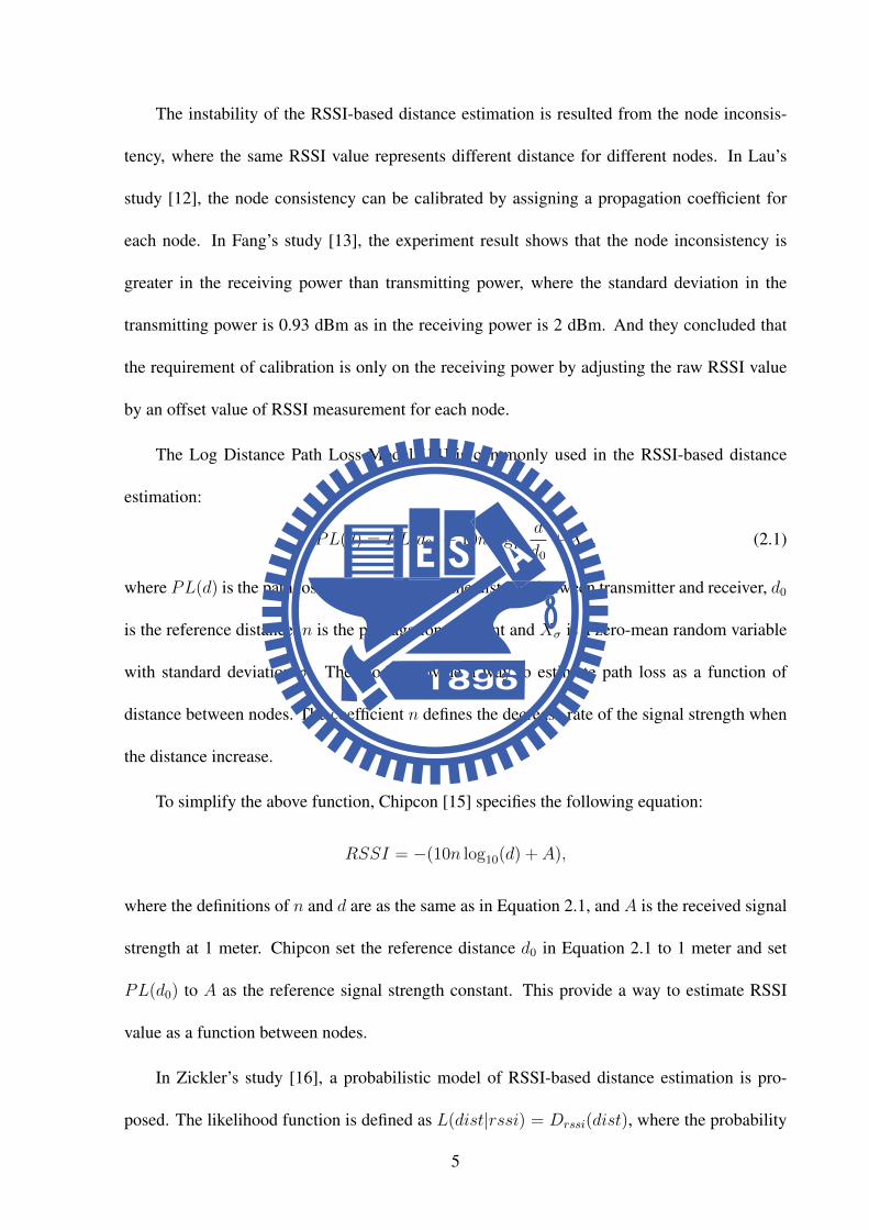
The Log Distance Path Loss Model [14] is commonly used in the RSSI-based distance
estimation:
PL(d) = PL(d0) + 10n log10
d
d0+Xσ, (2.1)
where PL(d) is the path loss at distance d, d is the distance between transmitter and receiver, d0
is the reference distance, n is the propagation constant and Xσ is a zero-mean random variable
with standard deviation σ. The model provide a way to estimate path loss as a function of
distance between nodes. The coefficient n defines the decrease rate of the signal strength when
the distance increase.
To simplify the above function, Chipcon [15] specifies the following equation:
RSSI = −(10n log10(d) + A),
where the definitions of n and d are as the same as in Equation 2.1, and A is the received signal
strength at 1 meter. Chipcon set the reference distance d0 in Equation 2.1 to 1 meter and set
PL(d0) to A as the reference signal strength constant. This provide a way to estimate RSSI
value as a function between nodes.
In Zickler’s study [16], a probabilistic model of RSSI-based distance estimation is pro-
posed. The likelihood function is defined as L(dist|rssi) = Drssi(dist), where the probability
5
distribution is modeled as
Drssi(dist) =max(0, σ −max(0, |dist− µ| − τ))
σ,
where dist is the distance, µ is the mean of the distribution, τ is the radius of the trapezoid’s
uniform center component, and σ is the radius of the trapezoid’s linear falloff component. Zick-
ler’s model provide a way to estimate the probability of a receiving node at a particular distance
from the transmitter as a function of the given RSSI value.
2.2 Anchor-based Localization Algorithms
Anchor-based localization algorithms usually work with RSSI-based distance estimation,
since the location computing is based on the distances between anchor nodes and sensor nodes.
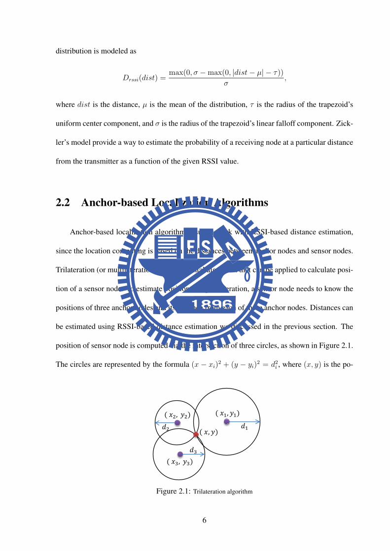
Trilateration (or multilateration), a fundamental algorithm that can be applied to calculate posi-
tion of a sensor node. To estimate position using trilateration, a sensor node needs to know the
positions of three anchor nodes and its distance from each of these anchor nodes. Distances can
be estimated using RSSI-based distance estimation we discussed in the previous section. The
position of sensor node is computed via the intersection of three circles, as shown in Figure 2.1.
The circles are represented by the formula (x − xi)2 + (y − yi)2 = d2i , where (x, y) is the po-
.
L
Control Server L
L
𝐀𝑖
𝐒𝑗
( 𝑥1,𝑦1) ( 𝑥2, 𝑦2)
( 𝑥3, 𝑦3)
( 𝑥,𝑦) 𝑑1 𝑑2
𝑑3
Figure 2.1: Trilateration algorithm
6

sition of sensor node, (xi, yi) is the position of the ith anchor node, and di is the distance from
the ith anchor node to the sensor node. Furthermore, if more than three anchor nodes are avail-
able, it becomes to a overdetermined system. The overdetermined system usually has more than
one solution. Gradient descent can be applied to obtain the positions of the non-anchor node
achieving the least square error.
Other algorithms like bounding box [17] and probabilistic approach [18] can also use to
compute node positions in anchor-based algorithms. The bounding box algorithm uses squares
instead of circles (in trilateration algorithm) to bound the possible position of a sensor node.
The probabilistic approach algorithm models the errors in distance estimation between anchor
nodes and sensor nodes as normal random variables for calculating the probable position of a
sensor node. However, due to the computing complexity, the trilateration algorithm is more
popular to be applied in WSN.
Due to the power consumption and localization accuracy, the anchor-based algorithms are
the most popular localization algorithms in WSN. The anchor-based algorithms locate sensor
nodes under the assumption of the precise position of anchor nodes. If the position of anchor
nodes are configured inaccurately, the incremented error may seriously influence on the sensor
locating accuracy. Hence, the precise anchor node position is the main requirement of anchor-
based algorithms.
2.3 Inertial Navigation System
Inertial navigation, a self-contained navigation technique, adopts accelerometers and gy-
roscopes to track the position and orientation of an object relative to a known starting point,
orientation and velocity [19]. Inertial Measurement Units (IMUs) typically use three orthog-
7

onal gyroscopes and three orthogonal accelerometers to measure angular velocity and linear
acceleration respectively. The advances in the construction of MEMS devices in recent years
have made it possible to manufacture small and light inertial navigation systems. These ad-
vances have widened the applications to include human and animal motion capture. The iner-
tial navigation system estimates the position and orientation of a moving object by continuously
tracking the output from a number of sensors in the IMUs attached to the object [20].
2.4 Procrustes Analysis
Procrustes analysis is a well-known technique to transform one set of data to represent
another set of data as closely as possible [21][22]. The Procrustes analysis provides least squares
matching of two or more set of data for the multidimensional rotating, translating, and uniformly
scaling of different matrix configurations. It is first applied in the factor analysis, and has
become a popular method of shape analysis [23]. Moreover, the Procrustes analysis is applied
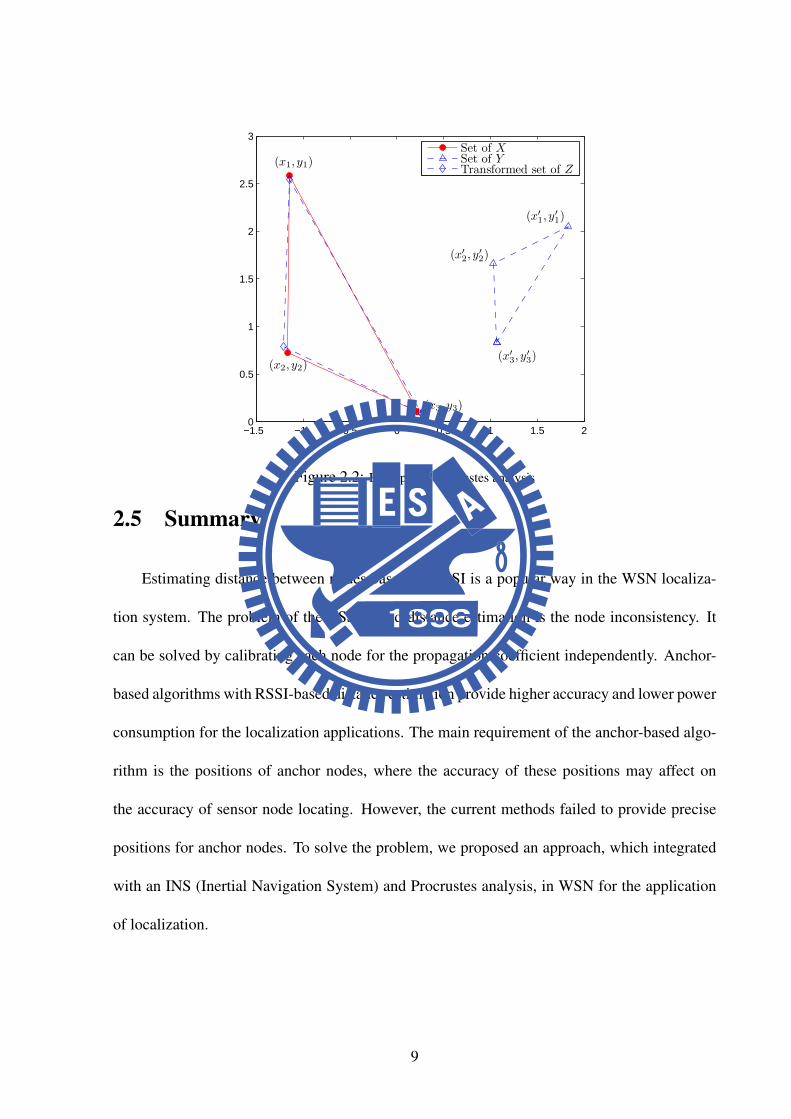
to coordinate transformation [24]. Specifically, given a set of reference coordinates, X , and a
set of coordinates to be transformed, Y . Procrustes gives a transformation that minimizes the
difference between X and the transformed coordinates, Z, as in the equation as
Z = s× Y ×R + t.
In the equation, s is the scalar, R is the rotation/reflection, and t is the translation, each of them
is determined by the Procrustes analysis to minimize the sum of squared errors between X and
transformed Z.
For example, the given coordinates set X = {(x1, y1); (x2, y2); (x3, y3)} and the coordi-
nates set to be transformed Y = {(x′1, y′1); (x′2, y′2); (x′3, y
′3)}. The Procrustes analysis gives the
transformed set Z with scaling, rotating, and translating as shown in Figure 2.2.
8
−1.5 −1 −0.5 0 0.5 1 1.5 20
0.5
1
1.5
2
2.5
3
Set of XSet of YTransformed set of Z
(x3, y3)
(x′3, y
′3)
(x1, y1)
(x2, y2)
(x′2, y′2)
(x′1, y′1)
Figure 2.2: Example of Procrustes analysis
2.5 Summary
Estimating distance between nodes based on RSSI is a popular way in the WSN localiza-
tion system. The problem of the RSSI-based distance estimation is the node inconsistency. It
can be solved by calibrating each node for the propagation coefficient independently. Anchor-
based algorithms with RSSI-based distance estimation provide higher accuracy and lower power
consumption for the localization applications. The main requirement of the anchor-based algo-
rithm is the positions of anchor nodes, where the accuracy of these positions may affect on
the accuracy of sensor node locating. However, the current methods failed to provide precise
positions for anchor nodes. To solve the problem, we proposed an approach, which integrated
with an INS (Inertial Navigation System) and Procrustes analysis, in WSN for the application
of localization.
9
Chapter 3
Related Work
In this chapter, we first introduce the method of reverse locating anchor nodes in WSN.
We also discuss the pros and cons of existing methods of reversely locating Wi-Fi access points
(APs) location and make a brief summary.
3.1 Reversely Locating Anchor Nodes
The positions of anchor nodes in WSN are usually configured by GPS device or manual
setting. GPS is only suitable for outdoor environment and is an additional hardware that in-
creases the cost and the power consumption of nodes in WSN. Manually configuring the anchor
positions is a tedious procedure, which may involve artificial errors and is not suitable for a
large-scale wireless sensor network. Therefore, an efficient method is required to locate anchor
nodes in a WSN.
In 2008, Du [25] proposed a method to locate anchor nodes for WSN by magnetic dipoles
and GPS information in outdoor environment. They assumed that anchor nodes are all equipped
with magnetic dipoles and sprinkled evenly over the area. An aircraft with magnetic detection
instrument and GPS receiver then scans over the area and captures the magnetic dipole moment
with GPS information. Based on the magnetic dipole moment, the algorithm can obtain the
distance between the anchor nodes. However, such an algorithm requires additional modules
like magnetic dipole for each anchor nose. For adopting magnetic dipole, the algorithm works
10

well only in outdoor environments.
Most localization algorithms are designed for locating sensor nodes in a wireless sensor
network. None of them emphasize the reverse localization for anchor nodes. The existing
reverse localization algorithms are designed for finding Wi-Fi Access Point (AP) position in
Wi-Fi network. The positions of APs can then be used in a Wi-Fi-based Localization System
to locate Wi-Fi devices. Since APs in Wi-Fi network are similar to anchor nodes in WSN,
algorithms of finding AP positions can also used to locate anchor nodes in a WSN.
For indoor environments, Ekahau HeatMapper is a free tool to find Access Points (APs) in
Wi-Fi networks. HeatMapper is a good and free way to map APs in small Wi-Fi networks, and
the positions of APs are relatively accurate. However, it is not supported in the network with
other wireless protocols, like Zigbee and Bluetooth. After importing a floor plan image as a
map, a user carrying the laptop with HeatMapper installed walks slowly around the floor and
manually records the location of user on the map frequently. HeatMapper constantly collects
signal data from APs when the user walks around. Then, HeatMapper combines the signal
data, calculates and displays the locations of AP on the map. Figure 3.1 is a screen shot of
the Ekahau HeatMapper downloaded from www.ekahau.com. Six APs are found along with
the walking route. Figure 3.2 shows the real test of Ekahau HeatMapper in the second floor,
Engineering Building 5, Kuang-Fu campus of National Chiao Tung University. We can see
that the positions of Wi-Fi APs named EE207, EE208, and EE209 (deployed in room 207, 208,
and 209), as noted on the figure, are relatively accurate. But there still many Wi-Fi APs are not
localized by Ekahau HeatMapper. The disadvantage of the HeatMapper is the requirement of
floor plan. Without the floor plan, the positions are manually recorded with huge errors. Also,
the artificial error are included with the manual recording. Nevertheless, the method is still
worth for reference.
11

Figure 3.1: A screen shot of Ekahau HeatMapper (Source: www.ekahau.com)
3.2 Jones’ Method
In 2008, Jones [26] has developed a method to reversely locate Wi-Fi APs by a special
vehicle. The vehicle is equipped with an AP scanning device, a GPS device, a Wi-Fi radio
device and a Wi-Fi antenna system. The steps of the method is described as below:
1. The vehicle moves in a programmatic route.
2. The vehicle scans for Wi-Fi APs and collects RSSI values from the scanned APs.
3. The vehicle obtains the GPS coordinates through th GPS receiver.
4. The vehicle sends the collected RSSI and GPS coordinates to a control server (named
”Central Network Server” in the paper).
12
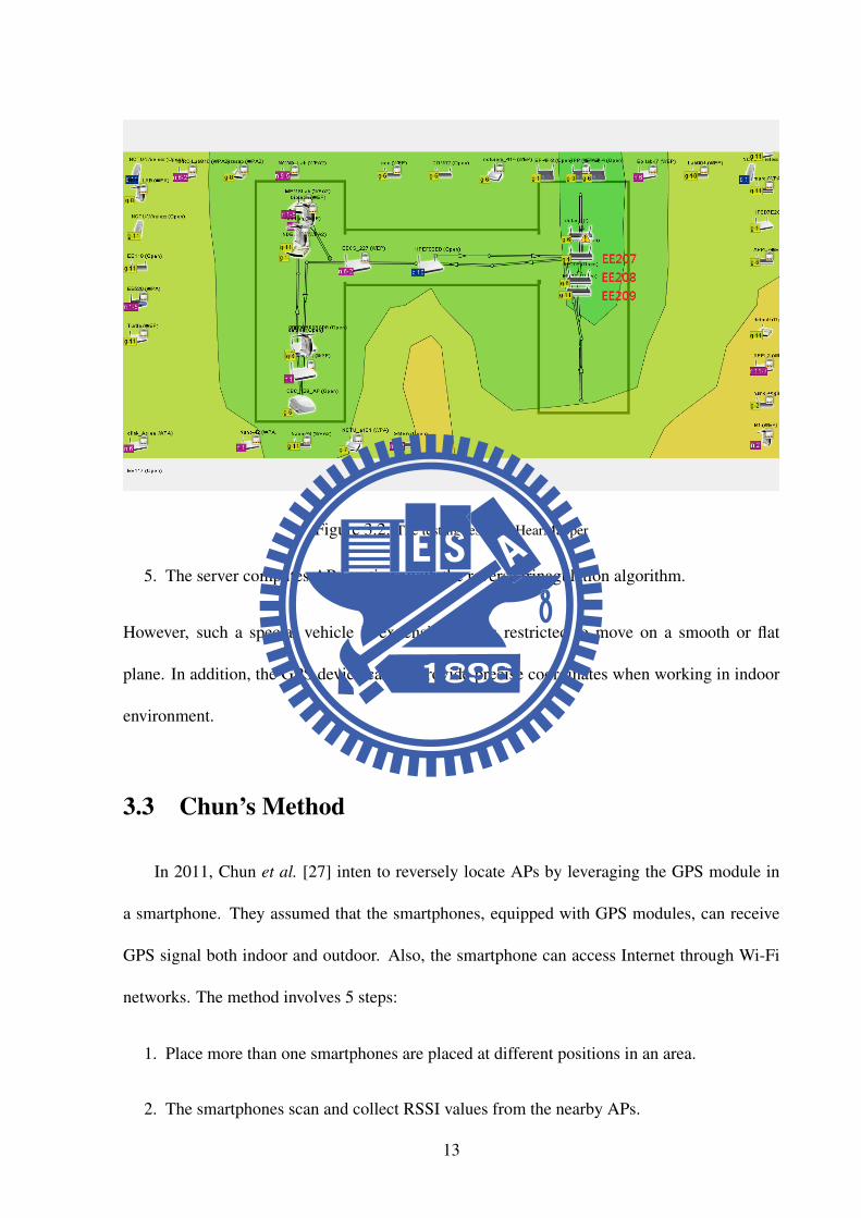
Figure 3.2: The testing result of HearMapper
5. The server computes AP locations with the reverse trinagulation algorithm.
However, such a special vehicle is expensive and is restricted to move on a smooth or flat
plane. In addition, the GPS device cannot provide precise coordinates when working in indoor
environment.
3.3 Chun’s Method
In 2011, Chun et al. [27] inten to reversely locate APs by leveraging the GPS module in
a smartphone. They assumed that the smartphones, equipped with GPS modules, can receive
GPS signal both indoor and outdoor. Also, the smartphone can access Internet through Wi-Fi
networks. The method involves 5 steps:
1. Place more than one smartphones are placed at different positions in an area.
2. The smartphones scan and collect RSSI values from the nearby APs.
13

3. The smartphones obtain GPS coordinates.
4. The smartphones upload the vector < x, y, r, AP MAC ID > to a control server, such
that the server can store the vector in the database. The parameters of x and y are the
x-axis and y-axis of the coordinates obtained from GPS and r is the RSSI value from AP
with the MAC identifier AP MAC ID.
5. The control server computes AP locations by Chun’s heuristic solution.
In their simulation, only one AP has been placed in the simulation area of 400 m × 300 m. The
coverage range of the AP is set to 100 meters. Assuming that the RSSI distortion is 20%, if 6
smartphones are used, the distance error ranges from 2m to 32m. The distance error reduces to
1m 9m if 15 smartphones are used. Their experiments shown an average distance error of 3.46
meter. The method overcomes the cost and unavailability of a customized vehicle, but suffers
from low accuracy when locating indoor APs.
3.4 Hansson’s Method
To solve the inaccuracy problem resulted from bad indoor GPS signals, in 2011, Hansson
and Tufvesson [20] have developed a method to reversely locate Wi-Fi AP by obtaining sensing
data from gyroscope, accelerometer, and magnetometer. First, an inertial navigation system
(INS) is developed on a smartphone with accelerometer, gyroscope, and magnetometer. The
INS is composed of an orientation tracker and a step detector and is used to record the walking
path of a user. Assume that the start position and orientation are known and fixed, the navigation
system can locate the AP with a global coordinates. In Hansson’s method, the error model of
the navigation system is presented with a linear functin of two variables e(t, d), where t is the
navigation time (in seconds) and d is the estimated distance (in meters). The coefficients of the
14

error model are defined as
e(t, d) = −0.2398 + 0.0152t+ 0.1081d, (3.1)
where e is the estimated error in meters. Hansson’s method is described as below:
1. A user carries a smartphone and walks around the testing area.
2. The smartphone continuously scans the Wi-Fi environment and determines the RSSI val-
ues for all nearby APs.
3. For each RSSI attained, the smartphone record the position by the navigation system.
4. The smartphone generates a vector mk = < AP MAC ID, r, x, y, e >, where x and y
are the coordinates and e is the estimated error of the position and r is the measured RSSI
value from AP with MAC identifier AP MAC ID. Then, the smartphone uploads the
vector to the control server.
5. The control server computes AP locations with the trilateration algorithm.
The overall system is shown in Figure 3.3. In their experiments, 6 APs are placed in a 60m ×
40m test field 18 walks are conducted. The results show that the position error of measured AP
positions and actual AP positions is from 0m to 10m and the average position error is 4.5m.
Phone
Phone
Phone
…
Server
mk
mk
mk
AP positions
Figure 3.3: The system architecture of Hansson’s method
15

Hansson has mentioned that the following restrictions that be fulfilled to obtain accurate
results:
• Known starting direction: The user is required to face to a known direction (e.g. north)
initially.
• Known starting position: The user is required to start at a known place.
With restrictions, the estimated positions of navigation system are always accurate at the start
point but obtain larger errors when getting far from the starting position. Thus, the error of
the located AP positions raises with the error of estimated positions of navigation system. The
restrictions also come with artificial errors when selecting the starting direction and position.
3.5 Summary
We introduce the common methods locating anchor nodes in a WSN localization system.
Since there are few researches in the localization of anchor nodes in WSN, we also introduce
and discuss the problems of the researches of finding AP locations in a Wi-Fi network. Each
of them has some drawbacks. Ekahau Heatmapper introduces artificial errors when recording
the walking path and requires a floor plan. Jone’s method suffers from the expensive and cus-
tomized vehicle, which is not easy to implement into other systems. Chun’s method suffers
from the poor GPS function in indoor environments. And Hansson’s method has undesirable
restrictions on the starting direction and position.
16

Chapter 4
Proposed Approach
In this chapter, we detail the proposed approach to reversely locate anchor nodes before
an anchor-based localization system is applied. Our approach estimates the anchor positions by
measuring RSSI measurements of wireless signal strength. With the measured anchor positions,
the existing anchor-based localization algorithms can locate moving nodes more precise. In our
approach, we define four types of devices and two phases for reverse anchor localization. In
this chapter, we first describe, and explain the proposed phases. In the end, we give a case study
adopting the proposed approach.
4.1 Preliminaries
In addition to anchor nodes and sensor nodes, we introduce two more devices used in out
approach, including training nodes and a control server.
• Anchor nodes, Ai: An anchor node, normally placed at a static/fix place, is used in a
localization system for localizing sensor nodes within a testing area. Ai represents the ith
anchor node, where i = 1, 2, · · · , I if maximum I anchor nodes are place in the testing
area.
• Sensor nodes, Sj: A sensor node, normally moving around an area and helping collect
data, should be tracked by a localization system. Sj represents the jth sensor node, where
j = 1, 2, · · · , J if at most J sensor node(s) are deployed in the field.
• Training nodes, Tk: In the proposed approach, some training nodes are used for re-
17

versely locating anchor nodes. Different from sensor nodes, a training node is assumed
to be equipped with gyroscope and accelerometer and is capable of recording its roaming
paths. Tk represents the kth training node, where k = 1, 2, · · · , K if at most K training
node(s) are used to reversely locate anchor nodes.
• Control server : The server is the center of the localization system that the all computing
take place. In our approach, the server is implemented in Matlab (The MathWorks, USA)
Version 7.10.0.499 (R2010a).
In our approach, we also assume that Ai, Tk and Sj can be existed in two parallel planes
with height difference h, as shown in Fig. 4.1, where three Ai are placed on the upper plane and
a Tk is moving on the lower plane. The height difference h between the two planes is fixed and
configured in the control server.
h
Ai
Tk
Phone
Phone
Phone
…
Server
mk
mk
mk
AP positions
𝐓1
𝐓2
𝐓K
…
Control Server
M
M
M
𝐀𝑖 positions
Calibration Training
Locate 𝐀𝑖 Localization
Locate 𝐓𝑘
𝐀𝑖 positions
𝐓𝑘’s CPC
𝐀𝑖’s CPC
Figure 4.1: Nodes in two parallel planes
4.2 Phases
There are two phases defined in our approach: calibration and training. The calibration
phase is to calibrate node inconsistency of the RSSI measurements between different nodes.
The training phase is to locate anchor nodes. The followings give the details of each phase.
18
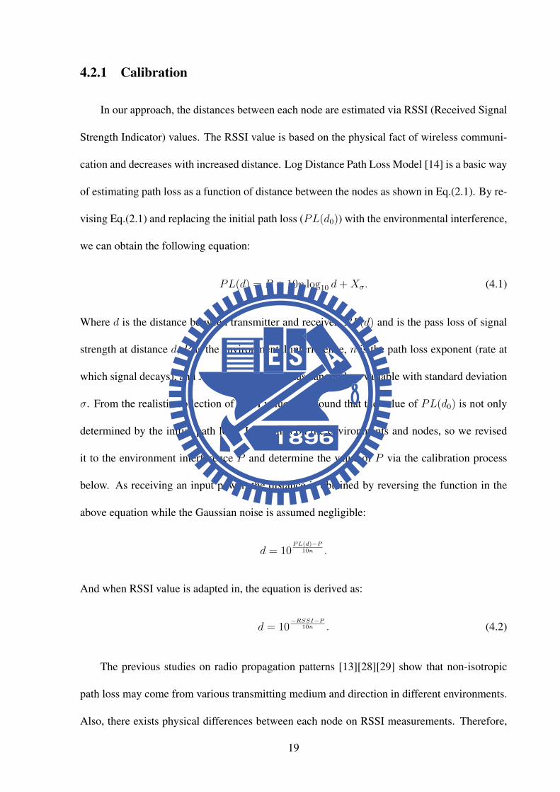
4.2.1 Calibration
In our approach, the distances between each node are estimated via RSSI (Received Signal
Strength Indicator) values. The RSSI value is based on the physical fact of wireless communi-
cation and decreases with increased distance. Log Distance Path Loss Model [14] is a basic way
of estimating path loss as a function of distance between the nodes as shown in Eq.(2.1). By re-
vising Eq.(2.1) and replacing the initial path loss (PL(d0)) with the environmental interference,
we can obtain the following equation:
PL(d) = P + 10n log10 d+Xσ. (4.1)
Where d is the distance between transmitter and receiver, PL(d) and is the pass loss of signal
strength at distance d, P is the environmental interference, n is the path loss exponent (rate at
which signal decays), and Xσ is a zero-mean Gaussian random variable with standard deviation
σ. From the realistic collection of RSSI values, we found that the value of PL(d0) is not only
determined by the initial path loss. It depends on the environments and nodes, so we revised
it to the environment interference P and determine the value of P via the calibration process
below. As receiving an input power, the distance is obtained by reversing the function in the
above equation while the Gaussian noise is assumed negligible:
d = 10PL(d)−P
10n .
And when RSSI value is adapted in, the equation is derived as:
d = 10−RSSI−P
10n . (4.2)
The previous studies on radio propagation patterns [13][28][29] show that non-isotropic
path loss may come from various transmitting medium and direction in different environments.
Also, there exists physical differences between each node on RSSI measurements. Therefore,
19
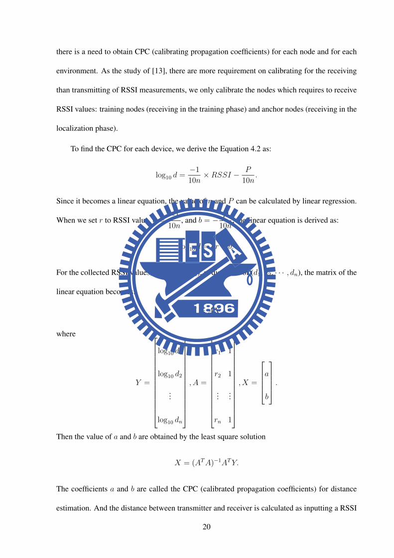
there is a need to obtain CPC (calibrating propagation coefficients) for each node and for each
environment. As the study of [13], there are more requirement on calibrating for the receiving
than transmitting of RSSI measurements, we only calibrate the nodes which requires to receive
RSSI values: training nodes (receiving in the training phase) and anchor nodes (receiving in the
localization phase).
To find the CPC for each device, we derive the Equation 4.2 as:
log10 d =−1
10n×RSSI − P
10n.
Since it becomes a linear equation, the value of n and P can be calculated by linear regression.
When we set r to RSSI value, a =−1
10n, and b = − P
10n, the linear equation is derived as:
log10 d = ar + b.
For the collected RSSI values,(r1, r2, · · · , rn), at distances of (d1, d2, · · · , dn), the matrix of the
linear equation becomes:
Y = AX,
where
Y =
log10 d1
log10 d2
...
log10 dn
, A =
r1 1
r2 1
......
rn 1
, X =
ab
.
Then the value of a and b are obtained by the least square solution
X = (ATA)−1ATY.
The coefficients a and b are called the CPC (calibrated propagation coefficients) for distance
estimation. And the distance between transmitter and receiver is calculated as inputting a RSSI
20

value to the equation:
d = 10(a×RSSI+b). (4.3)
4.2.2 Training
The objective of this phase is to locate anchor nodes and used the anchor nodes to locate
sensor nodes in the localization applications. In the phase, a set of training nodes Tk, (k =
1, 2, · · · , K) and the control server are used for the purpose, as illustrated in Figure 4.2. The
h
Ai
Tk
Phone
Phone
Phone
…
Server
mk
mk
mk
AP positions
𝐓1
𝐓2
𝐓𝐾
…
Control Server
M
M
M
𝐀𝑖 positions
Calibration Training
Locate 𝐀𝑖 Localization
Locate 𝐓𝑘
𝐀𝑖 positions
𝐓𝑘’s CPC
𝐀𝑖’s CPC
Figure 4.2: The architecture of training phase
two parts of the phase are separated, one part is running onK numbers of training nodes and the
other part is running on the control server. And M is the message that Tk sends to the control
server. The behavior of the training nodes and the server and the format of the message, M,
are discussed in the following sections. Before the training phase start, there are two system
parameters to be defined:
• K: the number of training nodes using for locating anchor nodes.
• MRC: the minumum RSSI collection for each Ai. It defines the minimum numbers of
RSSI value should be collected for an anchor node during the training of a Tk.
21

Training node, Tk
In the training phase, training nodes, Tk, are use to collect RSSI values from the anchor
nodes for locating anchor nodes. We assume that Tk knows the number of anchor nodes in the
test plane to be located. And each Tk has its own local coordinate system, Ck, and can record
its own position, Ck(x, y), at Ck. The position of Tk is recorded by a modified navigation
system from Hansson’s method [20]. Our modified navigation system has no restrictions on the
starting direction and position, since the restrictions of fixed starting direction and position are
only using for confirming all navigation systems are on the same coordinate system. The Ck is
substituted for the same coordinate system on the Tk. For each Tk, the local coordinate system,
Ck, is initialized when it starts: the starting position of Tk is defined to be the origin of Ck as
Ck(0, 0) and the starting direction of Tk is defined to be the positive x-axis of Ck as Ck(+, 0).
Thus, for K training nodes, there are K local coordinate systems: C1, C2, · · · , and CK . And
there are relations of rotation and translation between each Ck.
The behavior of the training nodes is illustrated in Figure 4.3. For each Tk, it initializes
Ck by the starting position and direction in the beginning. Then, user carries Tk walking around
the test plane. During the walking, Tk continuously communicate with Ai, which are deployed
in the test plane before the Tk starts, and determine RSSI values for all nearby Ai. As a RSSI
value is collected, the message of
M = (i, r,Ck(x, y), e)
is generated and sent to the control server, where i is the identifier of anchor node, r is the
measured RSSI value from Ai, Ck(x, y) is the position of Tk in Ck at receiving r , and e is
the estimated error of the position by the navigation system. Additionally, a variable for the
numbers of collected RSSI values from Ai is stored in Tk, which is noted as ni. To notify
the user when to stop the training, Tk examines the value of ni every time it changes. When
22

Initialize the starting position at 0,0
Move around and collect RSSI
Start training ( )
Collect RSSI from ?
NO
YES
Generate and send = ( ) to control server
MRCYES
End training ( )NO
Figure 4.3: The system flow of a training node
the value of ni for all Ai, i = 1, 2, · · · , I , are less than MRC, Tk notifies the user to keep
walking around. The user continue walking and measuring for anchor nodes until all ni values
are greater than or equal to MRC. As the ending of a training node, it sends an end message to
notice the server. And when the control server receives end messages from all Tk, it measures
the anchor positions at Ck.
However, the measured anchor positions cannot be used in the localization application yet,
since they are independent in each Ck and need to be integrated to a global coordinate system,
C̄. In our approach, this is handled on the server by the Procrustes Analysis.
23

Control Server
In the training phase, the control server measures the anchor positions after the training of
Tk. The behavior of the control server can be separated into two parts: after training of each
Tk and after training of all Tk, as illustrated in Figure 4.4. In the first part, the control server
Start
Import ’s CPC: (ak,bk)
Estimate distance of
Compute positions at
End
Start
Transform 1 to .
Derive positions at
End
Store (xi, yi) at
After training of each After training of all
Collect M from
Figure 4.4: The system flow of the server
computes Ai’s positions in each Ck. Then in the second part, the control server transforms all
Ck to a global coordinate system (C̄). At first, the Tk’s CPC, obtained in the calibration phase,
are imported to the control server as (ak, bk) for k = 1, 2, · · · , K. When a training node, Tk,
ends the training and sends the end message, the control server estimates distances by the RSSI
values in the message M from Tk. The distances are estimated by
d = 10(ak×r+bk),
where the uploading training node is Tk. As the training node and anchor nodes are in two
parallel planes with height difference h, the distances in two planes are projected into one plane
24
as d̂ by
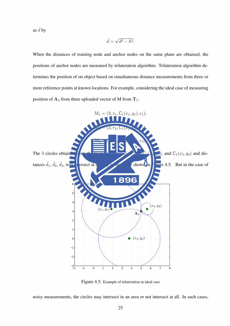
d̂ =√d2 − h2.
When the distances of training node and anchor nodes on the same plane are obtained, the
positions of anchor nodes are measured by trilateration algorithm. Trilateration algorithm de-
termines the position of on object based on simultaneous distance measurements from three or
more reference points at known locations. For example, considering the ideal case of measuring
position of A3 from three uploaded vector of M from T1:
M1 = (3, r1,C1(x1, y1), e1),
M2 = (3, r2,C1(x2, y2), e2),
M3 = (3, r3,C1(x3, y3), e3).
The 3 circles obtained from the training node C1(x1, y1), C1(x2, y2), and C1(x3, y3) and dis-
tances d̂1, d̂2, d̂3, will intersect at exactly on point, as shown in Figure 4.5. But in the case of
−2 −1 0 1 2 3 4 5 6 7 8−3
−2
−1
0
1
2
3
4
5
6
(x3, y3)
(x2, y2)
(x1, y1)A3
Figure 4.5: Example of trilateration in ideal case
noisy measurements, the circles may intersect in an area or not intersect at all. In such cases,
25

the trilateration algorithm gives the solution of the minimum error. For the measuring of an-
chor node Ai, assume that N measured d̂ at positions Ck(x, y), the matrices of trilateration are
formed as:
X =
s
xi
yi
, A =
1 −2x1 −2y1
1 −2x2 −2y2
......
...
1 −2xN −2yN
, B =
(d̂1)2− (x1)
2 − (y1)2
(d̂2)2− (x2)
2 − (y2)2
...
(d̂N)2− (xN)2 − (yN)2
,
where (xi, yi) is the estimated position of Ai in the Ck of Tk and s = xi2 + yi
2. We can write
the solution of Ai as X = A−1B only if N = 3 and A−1 exists. If N > 3, we can solve the
equation by X = A+B, where A+ is the pseudo-inverse of A. On solving, this gives the least
square error of the solution, and the Ai’s positions at Ck are the estimated as Ck(xi, yi).
The second part starts after the end of training for all Tk, the control server derives the
global coordinate system (C̄) and transforms K sets of Ai’s positions at Ck(xi, yi) into C̄.
To transform these sets to C̄, the Procrustes Analysis (PA) [22][30][31] is introduced to our
approach. PA is a well-known method to provide the least square matching of two matrices,
where the relation between two matrices is a linear transformation of translation, reflection,
orthogonal rotation, and scaling as we discussed in Chapter 2.4. In our approach, we assume
that the relative measured positions of Ai at Ck are similar. Thus, we can integrate K sets of
Ck(xi, yi) to C̄ base on the measured anchor positions of Ai. First, the Ai’s positions at Ck are
noted as Yk and Zk is the transformed set of Ai’s positions at C̄ from Ck. The C1 is set as the
C̄, which means Z1 = Y1, and Ck (k = 2, 3, · · · , K) are transformed to C̄. Since the relations
between each Ck are translation and rotation, the scalar factor is not involved in our approach.
Hence, the equation of the PA is modified as
Zk = Yk ×R + t,
26

−1 −0.5 0 0.5 1 1.5 2 2.5 3 3.5−0.5
0
0.5
1
1.5
2
2.5
3
A2
A1
A3
Figure 4.6: Y1 (Ai positions at C1)
−1 −0.5 0 0.5 1 1.5 2 2.5 3 3.5−0.5
0
0.5
1
1.5
2
2.5
3
A1
A2
A3
Figure 4.7: Y2 (Ai positions at C2)
where R and t are the rotation matrix and translation matrix respectively. The Procrustes anal-
ysis gives the Zk that
minR,t
E = Zk − Z1.
And after all Zk (k = 2, 3, · · · , K) are obtained, the average of Zk are the Ai positions, and are
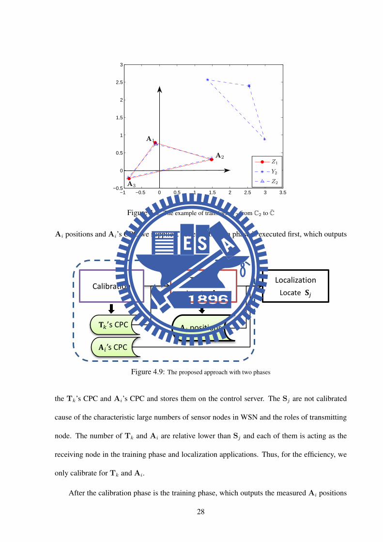
stored on the control server for the use of locating sensor nodes in the localization applications.
For example, three anchor nodes (A1,A2,A3) are located by two training nodes (T1,T2). The
measured Ai positions Y1 (Ai positions at C1) and Y2 (Ai positions at C2) are shown in Fig-
ure 4.6 and Figure 4.7. Since C̄ = C1 and Z1 = Y1, the Y2 is transformed to C̄ as Z2, which is
shown in Figure 4.8.
4.3 Proposed Approach
In Chapter 4.2, we’ve defined the two phases in our proposed approach. This section pro-
vides an overview of how the different phases work together in proposed system. The archi-
tecture is shown in Figure 4.9, two phases of calibration and training organize the complete
system and three types of data to be stored on the control server: Tk’s CPC, Ai’s CPC and Ai
positions. After our proposed system is the localization applications, which locate Sj with the
27
−1 −0.5 0 0.5 1 1.5 2 2.5 3 3.5−0.5
0
0.5
1
1.5
2
2.5
3
Z1
Y2
Z2
A2
A3
A1
Figure 4.8: The example of transform Y2 from C2 to C̄
Ai positions and Ai’s CPC we supplied. The calibration phase is executed first, which outputs
h
Ai
Tk
Phone
Phone
Phone
…
Server
mk
mk
mk
AP positions
𝐓1
𝐓2
𝐓𝐾
…
Control Server
M
M
M
𝐀𝑖 positions
Calibration Training
Locate 𝐀𝑖 Localization
Locate 𝐒𝑗
𝐀𝑖 positions
𝐓𝑘’s CPC
𝐀𝑖’s CPC
Figure 4.9: The proposed approach with two phases
the Tk’s CPC and Ai’s CPC and stores them on the control server. The Sj are not calibrated
cause of the characteristic large numbers of sensor nodes in WSN and the roles of transmitting
node. The number of Tk and Ai are relative lower than Sj and each of them is acting as the
receiving node in the training phase and localization applications. Thus, for the efficiency, we
only calibrate for Tk and Ai.
After the calibration phase is the training phase, which outputs the measured Ai positions
28

and stores them on the control server. In the training phase, there are two parameters to be
defined: K (used Tk numbers)and MRC (threshold of collected RSSI values). These two pa-
rameters affect the precision of measured Ai positions and the cost of the proposed approach.
Theoretically, the larger K, the more accurate at measured Ai positions, but the more cost due
to more devices of Tk are used. Similarly, the larger MRC, the more accurate at measured Ai
positions, but the longer duration of the training due to more RSSI values to be collected from
an Ai. Therefore, there is a need to decide the number of K and MRC for the appropriate set-
tings. For that, two experiments are designed to determine the appropriate number of the two
parameters for balancing the accuracy and the cost of time and funding.
As the Ai positions are measured, the localization application can be started. To make it
more clearly, we give a case of application is the following section.
4.3.1 Case Study
The localization application depends on the purpose of the system, which can be designed
for detecting, monitoring, or tracking. In this paper, the design of the localization application is
a simple localization system for testing the distance error of the estimated sensor positions by
the measured anchor positions. Before the phase, the anchor nodes are calibrated and Ai’s CPC
are stored on the control server. Different from acting as the transmitting node in the training
phase, anchor nodes play the receiving nodes in the localization application cause to the number
of anchor nodes is far less than sensor nodes and to obtain the simultaneous RSSI measurements
for localization. The measured anchor positions are stored in the server.
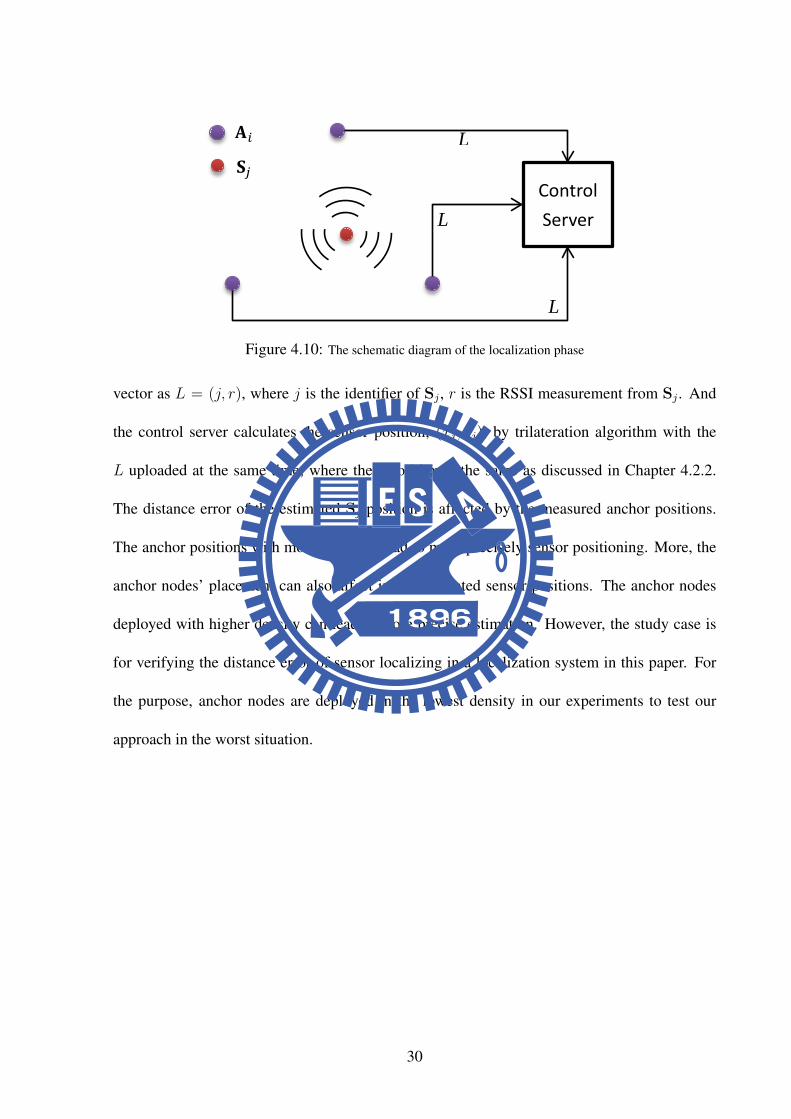
At first, the sensor nodes periodically broadcasting signals, as shown in Figure 4.10. As
the sensor node enters the field deployed with anchor nodes, the nearby anchor nodes, Ai,
receive the broadcast signals and determine the RSSI values and upload it to the server in a
29
L
Control Server L
L
𝐀𝑖
𝐒𝑗
Figure 4.10: The schematic diagram of the localization phase
vector as L = (j, r), where j is the identifier of Sj , r is the RSSI measurement from Sj . And
the control server calculates the sensor position, (xj, yj), by trilateration algorithm with the
L uploaded at the same time, where the algorithm is the same as discussed in Chapter 4.2.2.
The distance error of the estimated Sj position is affected by the measured anchor positions.
The anchor positions with more accuracy lead to more precisely sensor positioning. More, the
anchor nodes’ placement can also affect in the estimated sensor positions. The anchor nodes
deployed with higher density can lead to more precise estimation. However, the study case is
for verifying the distance error of sensor localizing in a localization system in this paper. For
the purpose, anchor nodes are deployed in the lowest density in our experiments to test our
approach in the worst situation.
30
Chapter 5
Experiments
In this chapter, we first introduce the experiment platform and its configuration, then we
conduct several experiments to evaluate the calibration phase in our proposed approach. First,
we introduce the hardware and environment in our experiments, and we verify the node in-
consistency of the RSSI measurements by the experiment of 10 receiving nodes and 1 trans-
mitting node. Then we estimate the CPC (calibrated propagation coefficients, discussed in
Chapter 4.2.1) for each receiving node and test the distance estimation error with the CPC. At
the end, we analysis the RSSI characteristics of the collected data.
5.1 Hardware and Experiment Environment
The hardware device used in the experiments is composed of a MCU (MSP430FS5438)
and a RF chip (CC2500EMK). The wireless network protocol is SimpliciTI [32], which is
a TI (Texas Instruments) proprietary low-power RF network protocol. The experiments take
place at the hallway of second floor, Engineering Building 5, Kuang-Fu campus of NCTU.
The transmitting node is set to be an anchor node, A1, and the 10 receiving nodes are set to
be training nodes, Tk, (k = 1 · · · 10). And the nodes are placed on the ground during the
experiments.
31
5.2 Node Inconsistency
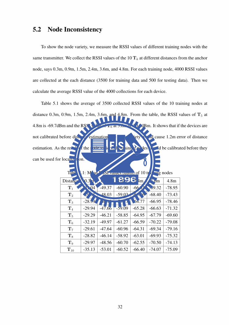
To show the node variety, we measure the RSSI values of different training nodes with the
same transmitter. We collect the RSSI values of the 10 Tk at different distances from the anchor
node, says 0.3m, 0.9m, 1.5m, 2.4m, 3.6m, and 4.8m. For each training node, 4000 RSSI values
are collected at the each distance (3500 for training data and 500 for testing data). Then we
calculate the average RSSI value of the 4000 collections for each device.
Table 5.1 shows the average of 3500 collected RSSI values of the 10 training nodes at
distance 0.3m, 0.9m, 1.5m, 2.4m, 3.6m, and 4.8m. From the table, the RSSI values of T5 at
4.8m is -69.7dBm and the RSSI value of T6 at 3.6m is -70.2dBm. It shows that if the devices are
not calibrated before distance estimation, the node variety would cause 1.2m error of distance
estimation. As the result of the node variety, the training nodes should be calibrated before they
can be used for localization.
Table 5.1: Mean RSSI values (dBm) of 10 training nodes
Distance 0.3m 0.9m 1.5m 2.4m 3.6m 4.8mT1 -31.04 -49.37 -60.90 -66.93 -69.32 -78.95T2 -29.81 -48.03 -59.03 -65.86 -68.40 -73.43T3 -28.99 -46.11 -59.47 -64.77 -66.95 -78.46T4 -29.94 -47.66 -59.09 -65.28 -66.63 -71.32T5 -29.29 -46.21 -58.85 -64.95 -67.79 -69.60T6 -32.19 -49.97 -61.27 -66.59 -70.22 -79.08T7 -29.61 -47.64 -60.96 -64.31 -69.34 -79.16T8 -28.82 -46.14 -58.92 -63.01 -69.93 -75.32T9 -29.97 -48.56 -60.70 -62.55 -70.50 -74.13T10 -35.13 -53.01 -60.52 -66.40 -74.07 -75.09
32

5.3 CPC Estimation and Test
As discussed in calibration phase in Chapter 4.2.1, the CPC (calibrated propagation coeffi-
cient) is the parameters we need for distance estimation in the localization. Following the data
of Table 5.1, we calculate the CPC, ak and bk, for Tk as the method in Chapter 4.2.1. The ak
and bk for Tk are shown in Table 5.2.
Table 5.2: The propagation coefficient ak and bk of 10 training nodes
Device ak bk
T1 -0.0258 -1.3307T2 -0.0275 -1.3690T3 -0.0250 -1.2294T4 -0.0283 -1.3972T5 -0.0278 -1.3581T6 -0.0263 -1.3735T7 -0.0250 -1.2556T8 -0.0258 -1.2659T9 -0.0270 -1.3527T10 -0.0293 -1.5714
Then, 3000 testing data (500 measurements at 6 distances) are used for testing the distance
estimation. The distance is measured by Equation 4.3, where a and b are replaced by ak and bk
as:
d = 10(ak×r+bk),
where r is the testing data of measured RSSI value by Tk (500 measurements at 6 distances) and
d is the estimated distance. For the comparison of non-calibrated distance estimation, we used
the CPC of T1, a1 and b1, for the represent of non-calibrated propagation coefficients. For the
test of each Tk, distances are estimated through the calibrated coefficients ak and bk and also the
non-calibrated coefficients a1 and b1. The distance estimation error with calibration and without
calibration of each device is shown in Table 5.3. The calibration reduced 21.3% of distance
33
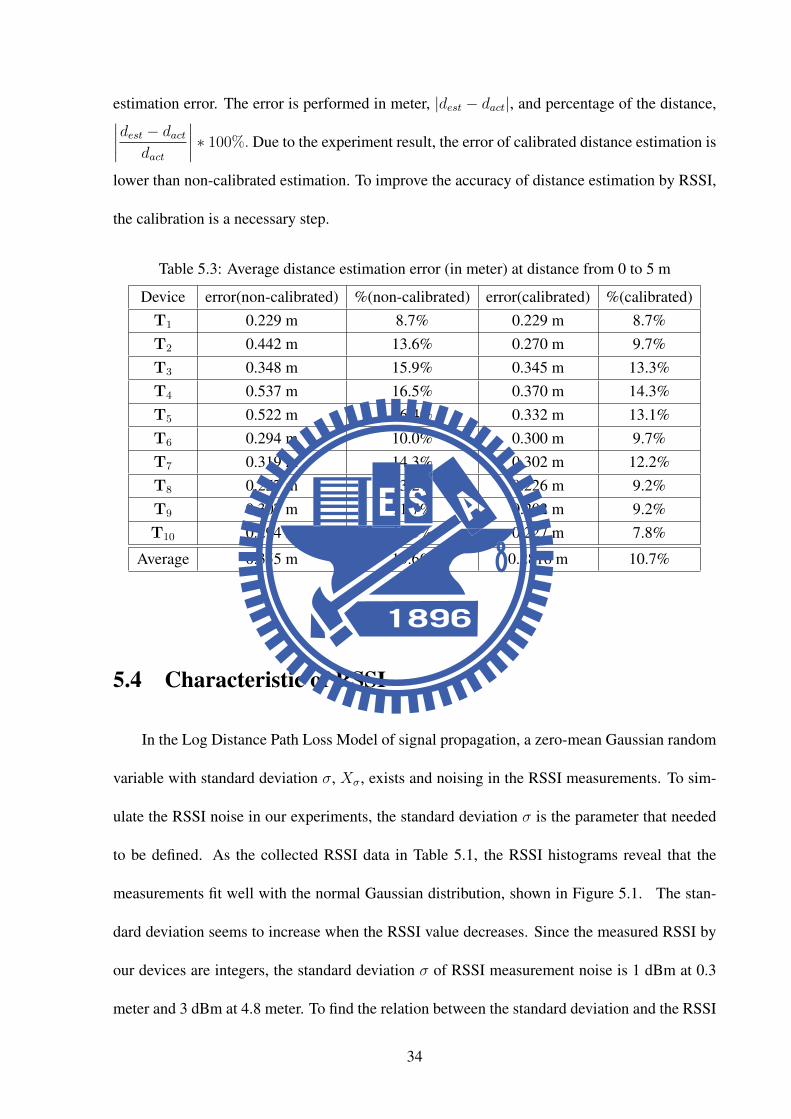
estimation error. The error is performed in meter, |dest − dact|, and percentage of the distance,∣∣∣∣dest − dactdact
∣∣∣∣ ∗ 100%. Due to the experiment result, the error of calibrated distance estimation is
lower than non-calibrated estimation. To improve the accuracy of distance estimation by RSSI,
the calibration is a necessary step.
Table 5.3: Average distance estimation error (in meter) at distance from 0 to 5 m
Device error(non-calibrated) %(non-calibrated) error(calibrated) %(calibrated)T1 0.229 m 8.7% 0.229 m 8.7%T2 0.442 m 13.6% 0.270 m 9.7%T3 0.348 m 15.9% 0.345 m 13.3%T4 0.537 m 16.5% 0.370 m 14.3%T5 0.522 m 16.4% 0.332 m 13.1%T6 0.294 m 10.0% 0.300 m 9.7%T7 0.319 m 14.3% 0.302 m 12.2%T8 0.257 m 13.2% 0.226 m 9.2%T9 0.307 m 11.7% 0.202 m 9.2%T10 0.294 m 15.5% 0.227 m 7.8%
Average 0.355 m 13.6% 0.2816 m 10.7%
5.4 Characteristic of RSSI
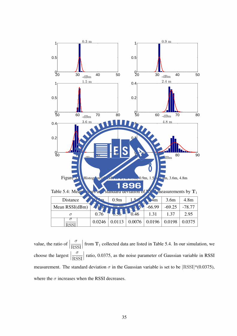
In the Log Distance Path Loss Model of signal propagation, a zero-mean Gaussian random
variable with standard deviation σ, Xσ, exists and noising in the RSSI measurements. To sim-
ulate the RSSI noise in our experiments, the standard deviation σ is the parameter that needed
to be defined. As the collected RSSI data in Table 5.1, the RSSI histograms reveal that the
measurements fit well with the normal Gaussian distribution, shown in Figure 5.1. The stan-
dard deviation seems to increase when the RSSI value decreases. Since the measured RSSI by
our devices are integers, the standard deviation σ of RSSI measurement noise is 1 dBm at 0.3
meter and 3 dBm at 4.8 meter. To find the relation between the standard deviation and the RSSI
34
20 30 40 500
0.5
1
-dBm
0.3 m
20 30 40 500
0.5
1
-dBm
0.9 m
50 60 70 800
0.5
1
-dBm
1.5 m
50 60 70 800
0.2
0.4
-dBm
2.4 m
60 70 80 900
0.2
0.4
-dBm
3.6 m
60 70 80 900
0.2
0.4
-dBm
4.8 m
Figure 5.1: Histogram of RSSI of T1 at 0.3m, 0.9m, 1.5m, 2.4m, 3.6m, 4.8m
Table 5.4: Mean values and standard deviation of RSSI measurements by T1
Distance 0.3m 0.9m 1.5m 2.4m 3.6m 4.8mMean RSSI(dBm) -31.04 -49.40 -60.85 -66.99 -69.25 -78.77
σ 0.76 0.56 0.46 1.31 1.37 2.95∣∣∣ σ
RSSI
∣∣∣ 0.0246 0.0113 0.0076 0.0196 0.0198 0.0375
value, the ratio of∣∣∣ σ
RSSI
∣∣∣ from T1 collected data are listed in Table 5.4. In our simulation, we
choose the largest∣∣∣ σ
RSSI
∣∣∣ ratio, 0.0375, as the noise parameter of Gaussian variable in RSSI
measurement. The standard deviation σ in the Gaussian variable is set to be |RSSI|*(0.0375),
where the σ increases when the RSSI decreases.
35

Chapter 6
Simulation & Comparison
In this chapter, we verify the correctness of our proposed approach on the anchor nodes
locating in the training phase and the sensor nodes locating in the localization phase. Due to
the serious signal interferences in the campus buildings (Figure 3.2 shows the interference of
second floor Engineering Building 5, Kuang-Fu campus of NCTU), we conduct the experiments
with Matlab for the verification. The real signal propagation data from the experiments in the
above chapter is involved to make our simulation closer to actual situation.
6.1 Setup
To justify that the proposed algorithm is practical, we simulate the algorithm via Matlab
(The MathWorks, USA) Version 7.10.0.499 (R2010a). The simulation area is 15m × 13m,
which simulates the second floor, Engineering Building 5, Kuang-Fu campus of NCTU. The
anchor nodes are placed in the lowest density, which ensures everywhere has 3 anchor coverage.
For the device and the protocol we used in Chapter 5, the RSSI value fluctuated seriously over
5 meters. Therefore, we assume the maximum transmitting range of the wireless signal is 5
meters. Due to the transmitting range, we deployed 23 anchor nodes(Ai, I = 23) in the area,
where the distance between Ai is 3.75 meters. The environment is shown in Figure 6.1, where
black circles are the location of anchor nodes. If the other protocol is substitute in, such as
Bluetooth or Zigbee, the transmitting range can be set to 10 meters or longer and the less anchor
nodes can be used in the same area. In the simulation, all the anchor nodes and training nodes
are assumed to be placed in two parallel plane: anchor nodes are placed at the ceiling, training
36

−6 −4 −2 0 2 4 6
−6
−4
−2
0
2
4
6
The simulation area
15 m
13 m
Figure 6.1: The simulation area
nodes and sensor nodes are hung in front of the chest of users. The height between the ceiling
and the chest of users are assumed to be 1.5 meter (all users are at the same height).
6.2 Design
To verify our approach, four experiments are designed in this paper. Three experiments are
designed for the testing of training phase and finding the appropriate number of two parameters
in the training phase. And one experiment is designed for the testing of localization phase.
Exp#1: Removing the starting restrictions
The objective of Exp#1 is to verify that the restrictions of starting direction and starting
position can be removed in our algorithm. Two conditions of training phase are designed: one
is that all training nodes are started with restrictions, and the other is without restrictions. To
37

compare the distance error of estimated anchor positions of two conditions, the threshold of
collected RSSI values is set to the same value. The distance error is compared at different
settings of the training node numbers.
Exp#2: Finding the proper setting of K
To determine the number of training nodes used in the training phase, we design the exper-
iment to measuring anchor positions with different numbers of K. Theoretically, the distance
error decreases as K increase since the noise of RSSI measurements and navigation measure-
ments are averaged. However, the larger K means the more cost due to more devices are used.
Therefore, there is a need to find an appropriate K to balance the cost and accuracy. The range
of K varies from 1 to 20. And we list the distance error of estimated anchor positions with K
for analysing. The threshold of collected RSSI value, MRC, is set to the same value.
Exp#3: Finding the proper setting of MRC
To determine the MRC in the training phase, we design the experiment to measuring anchor
positions with different MRC. It is used to determine when a training of a training node is done:
for all ni are over MRC, where ni is the number of measured RSSI values of each anchor nodes,
Ai (i = 1, 2, · · · , I). Theoretically, the distance error decreases as MRC increases since to the
averaging of the noise. But the larger MRC means the longer period of the training phase, which
consumes more power. Therefore, there is a need to find an appropriate number of MRC. Since
the trilateration needs at least three measurements to localize the target, MRC is set to varying
from 3 to 8 in the experiment.
38

Exp#4: Locating sensor nodes
The objective of Exp#4 is to evaluate the localization error by using measured anchor po-
sitions. First, the anchor positions are measured through the training phase with the appropriate
settings determined in Exp#2 (K) and Exp#3 (MRC) and training nodes start from different
directions and positions. After the anchor positions are measured, the sensor nodes, Sj , are
randomly set in the area. The positions of Sj are measuring through the localization phase. For
comparison, the localization with actual anchor positions, which are manually configured, is
also tested in this experiment.
6.3 Noise Source
Before we start our simulation, there are two sources of noise that may influence the accu-
racy of the measured anchor positions in our approach:
• Navigation system: the position estimation error of the navigation.
• RSSI measurement: the physical interference on path loss of wireless signal.
To make our experiment closer to actual situation, the noises must be inducted into our experi-
ments.
6.3.1 Noise of Navigation System
To simulate the noise of the navigation system, the design of Hansson [20] is inducted into
our experiments. The estimating error model defined by Hansson is shown in Equation 3.1.
In the Equation 3.1, there are two coefficients need to be defined in our experiments. The
coefficient t is the time since the start of the navigation in seconds. It is determined by the
39
total walking length and the walking speed. The total walking length is calculated from the
message sent by training node, and the walking speed is set as 1.4 m/s, according to the studies
of [33][34]. The coefficient d is the estimated distance to the start point in meters. It is
determined by the distance from current uploading position of training node to the origin in the
local coordinates (the start point of training node is defined as the origin in local coordinates).
Therefore, when the current estimated position of navigation system is Ck(x, y) at Ck, the error
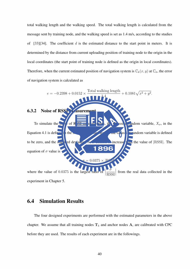
of navigation system is calculated as
e = −0.2398 + 0.0152× Total walking length
1.4+ 0.1081
√x2 + y2.
6.3.2 Noise of RSSI Measurement
To simulate the noise of RSSI measurements, the Gaussian random variable, Xσ, in the
Equation 4.1 is defined in the simulation. The mean of the Gaussian random variable is defined
to be zero, and the standard deviation, σ, is defined to increase with the value of |RSSI|. The
equation of σ value is
σ = 0.0375× |RSSI| ,
where the value of 0.0375 is the largest ratio of∣∣∣ σ
RSSI
∣∣∣ from the real data collected in the
experiment in Chapter 5.
6.4 Simulation Results
The four designed experiments are performed with the estimated parameters in the above
chapter. We assume that all training nodes Tk and anchor nodes Ai are calibrated with CPC
before they are used. The results of each experiment are in the followings.
40
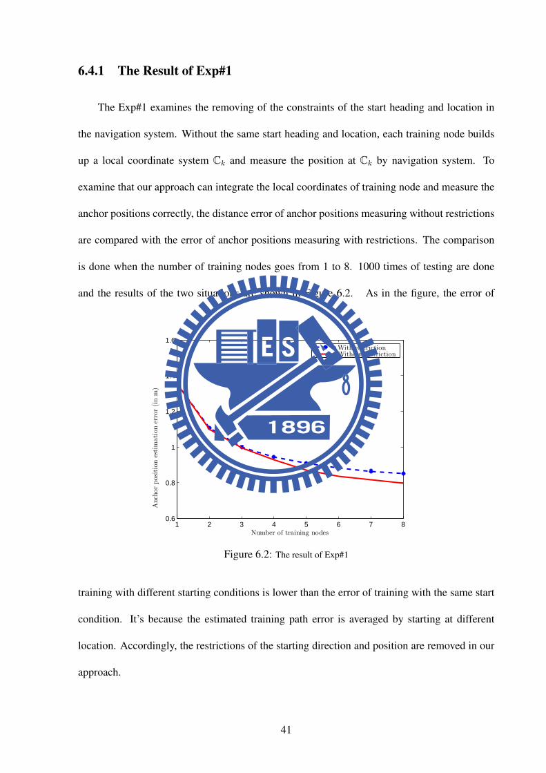
6.4.1 The Result of Exp#1
The Exp#1 examines the removing of the constraints of the start heading and location in
the navigation system. Without the same start heading and location, each training node builds
up a local coordinate system Ck and measure the position at Ck by navigation system. To
examine that our approach can integrate the local coordinates of training node and measure the
anchor positions correctly, the distance error of anchor positions measuring without restrictions
are compared with the error of anchor positions measuring with restrictions. The comparison
is done when the number of training nodes goes from 1 to 8. 1000 times of testing are done
and the results of the two situations are shown in Figure 6.2. As in the figure, the error of
1 2 3 4 5 6 7 80.6
0.8
1
1.2
1.4
1.6
Number of training nodes
Anchorpositionestimationerror(inm)
With restrictionWithout restriction
Figure 6.2: The result of Exp#1
training with different starting conditions is lower than the error of training with the same start
condition. It’s because the estimated training path error is averaged by starting at different
location. Accordingly, the restrictions of the starting direction and position are removed in our
approach.
41

6.4.2 The Result of Exp#2
The Exp#2 finds the appropriate number of training nodes, K, using in the training phase.
In the experiment, 1 to 20 training nodes (K = 1, 2,· · · , 20) are used to measure the anchor
positions. 1000 times of tests are performed and the distance error of anchor positions by
different numbers of K is shown in Figure 6.3. We can see that the distance error of using only
2 4 6 8 10 12 14 16 18 200.6
0.8
1
1.2
1.4
Number of training nodes
Anchorpositionestimationerror(inm)
Figure 6.3: Simulation of reverse localization with different numbers of training nodes
one training node is about 1.37 meters. When one training node is added in the training phase,
the distance error decrease fast when using more training nodes until using 8 training nodes,
where the improve percentage are more than 2% as shown in Table 6.1. When the number of
training nodes is over 8, the localization error decrease slowly ( less than 2%). Therefore, we
conclude that 8 training nodes are proper for training phase, and the expected localization error
is below 0.8 meters.
42

Table 6.1: Improve percentage of adding 1 training node at each K
K 1 2 3 4 5 6 7 8 9Distance error (m) 1.37 1.10 1.00 0.93 0.87 0.83 0.80 0.78 0.77
Improvement - 19.7% 9.1% 7.0% 6.5% 4.6% 3.6% 2.5% ≤ 2%
6.4.3 The Result of Exp#3
The Exp#3 determines the proper setting of MRC for the training phase. In the experiment,
MRC are set from 3 to 8 in the training phase for measuring anchor positions. For the tests,
8 training nodes (K = 8) are used since the result of Exp#2 shows that it is the appropriate
number for the training phase. 1000 times of testing are performed and the distance error of
anchor positions by the different number of MRC is listed in Table 6.2. The distance error is
1.1228 meters when MRC is set to 3, which is too large for using in the localization phase.
When MRC is set to 4, the distance error is less than 0.8 meters. For the larger MRC, the
distance error decreases but with little improvement, where the distance errors are all between
0.7 and 0.8 meters. Therefore, we conclude that the MRC = 4 is the appropriate setting for the
training phase. Which means a training node needs to receive at least four RSSI measurements
from each anchor nodes.
Table 6.2: Average error of measuring anchor nodes position by different MRC
MRC 3 4 5 6 7 8Distance error 1.1228 m 0.7877 m 0.7827 m 0.7754 m 0.7413 m 0.7378 m
6.4.4 The Result of Exp#4
The Exp#4 evaluates the performance of the sensor nodes locating in the localization phase
using measured anchor positions by our approach. The settings for training phase are K = 8
43

and MRC = 4, as the result of Exp#2 and Exp#3. After the training phase, the measured anchor
positions are used in the localization phase. And as the comparison, the localization phase is
also performed with actual anchor positions. For each test, 100 sensor nodes are randomly
placed in the 15m×13m field. And 1000 tests are performed with the simulation. First, we
examine the result of the measured anchor positions in training phase. The distance error range
between the measured anchor positions and actual anchor positions of the 1000 tests is from
0.544 to 1.563 meters, where the mean is 0.78 meters. Then the result of sensor nodes locating
using measured anchor positions and using actual anchor positions are shown in Table 6.3. The
distance error with actual anchor positions is 0.67 meter as the error with measured anchor
positions is 0.732 meter. The localization using measured anchor positions by our approach
increases 0.062 meter in localization error, which only increases 9.25% of error when using
actual anchor positions.
Table 6.3: Distance error of sensor nodes locating in the localization phase
Localization with Distance error Standard deviationActual anchor positions 0.670 m 0.042 m
Measured anchor positions 0.732 m 0.074 m
6.5 Comparison
In this section, we give the comparison of our proposed approach and other methods on the
RSSI measurement, additional hardware and restrictions, and power consumption.
44

RSSI measurements
First, we discuss the RSSI measurement in our proposed approach and other three methods.
In our approach, the CPC (calibrated propagation coefficient) of each node that requires to
measure RSSI value are given to the control server to improve the distance estimation. As
the result in Chapter5, the error of distance estimation with calibration is 23.5% less than the
estimation without calibration. In Jones’ method, since there is only one special vehicle for
collecting RSSI values, there is no need of calibration. The propagation model can be defined
just fit the special vehicle. In Chun’s and Hansson’s methods, there are several smartphones
using to collecting RSSI values but without calibration. As the result of node inconsistency
between devices, the distance estimation by RSSI value is less accurate than the estimation
with calibration.
Additional Hardware and Restriction
To compare with other approaches, we list the usage of additional hardware and the restric-
tions in each approach, as shown in Table 6.4. Both Jones’ and Chun’s methods required GPS
module, which is the most undesired component in WSN, to record the position of the device
that used for locating anchor nodes. The GPS module is expensive and power-consuming and
takes seconds to obtain the GPS coordinate, which is not suitable for the low-cost, low-power
sensors in WSN. Furthermore, since the GPS functions poorly indoors, it is not appropriate to
be used in the indoor applications.
Hansson’s and our proposed approaches remove the usage of GPS module and replace it
with small sensors to build an inertial navigation system. Benefit from the recent advances
of MEMS IC technology, the sensors such as accelerometer and gyroscope are manufactured
small and light that can be equipped on sensor nodes with low power-consuming. In the Hans-
45

Table 6.4: Comparison of the approachesApproach Jones’ Chun’s Hansson’s Proposed
AdditionalGPS module © © × ×
hardware SensorsAccelerometer × × © ©
Gyroscope × × © ©Magnetometer × × © ×
RestrictionsStart direction N/A N/A restricted non-restrictedStart position N/A N/A restricted non-restricted
©: Required× : Not required
son’s approach, the magnetometer is used to aid the orientation tracker. But the magnetometer
measurement is not reliable enough to used, they limit the usage of the magnetometer in the
orientation estimation. In our proposed approach, the magnetometer is removed from our nav-
igation system since the unreliable measurement and the magnetic disturbance in the indoor
environment. In Hansson’s approach, the navigation systems in each smartphone record posi-
tion in a global coordinate system and they collect all data from smartphones to compute the
position. For that, they restrict the start direction and position of the smartphones, which leads
to estimate positions are always with more error in the area apart from the start position than
the area near the start position. Consequently, we remove the restrictions and replace local co-
ordinate systems to the navigation systems on each training node. And by the training of each
training node, the positions of anchor nodes are first computed at local coordinate systems.
Then we integrate anchor positions in all local coordinate systems into a global coordinate sys-
tems. Thus, the errors of estimated positions are averaged over the test area and the users can
start the training with no restrictions.
46

Power Consumption
To compare the power consumption between approaches, we first list the power consump-
tion of GPS module, accelerometer and gyroscope. As shown in the Table 6.5, the power
Table 6.5: Power consumption of GPS, accelerometer, and gyroscope
Modules Power (mW)GPS (u-blox ANTARIS 4 in Openmoko) [35] 143.1
Accelerometer (ADXL335) [36] 1.24Gyroscope (LPR530AL + LY530ALH) [36] 40.59
consumption of GPS is 143.1 mW [35], where the GPS module is u-blox ANTARIS 4 in the
Openmoko Neo Freerunner (reversion A6) mobile phone. The power consumption of an inertial
navigation system using accelerometer and gyroscope is 41.83 mW [36], where the accelerom-
eter module is ADXL335 (triple-axis) and gyroscope modules are LPR530AL (pitch and roll
gyro) and LY530ALH (yaw gyro).
In our simulation, the average training time of a training node in the training phase is
60 seconds when MRC is set to 4. Assume that the GPS module and the accelerometer and
gyroscope modules are all power on during the training in each approach (GPS used in Jones’
and Chun’s methods and accelerometer and gyroscope used in Hansson’s and our proposed
approaches). The total energy consumption of Jones’ and Chun’s methods on the GPS module
are 8.58 Joule, where the Hansson’s method and our proposed approach are 2.5 Joule. The
energy consumption of accelerometer and gyroscope is 70% less than GPS module.
6.6 Summary
In this chapter, we demonstrate the proposed approach that can be applied to locate anchor
nodes in WSN. In the experiments, we evaluate the appropriate setting of K and MRC and then
47

used the setting to locate anchor nodes. Then we verified that the measured anchor positions
can be used to locate sensor nodes in the WSN localization applications. In conclusion, our
proposed approach provides a way to locate anchor nodes with fewer extra components than
other methods. And the localization error of sensor nodes with anchor positions measured by
our approach doesn’t increase much than the actual anchor positions.
48

Chapter 7
Conclusion and Future Work
In this research, taking Hansson’s method as a basis, we proposed a reverse localization
approach in WSN to locate anchor nodes. Our approach locates anchor nodes based on RSSI
values. An inertial navigation system is conducted with gyroscope and accelerometer to avoid
using GPS devices. Also, the coordinates transformation with Procrustes analysis is involved
for the training without restrictions on start direction and position. To demonstrate there are
no restrictions in our proposed approach, we design an experiment to test the anchor node
locating. The experiment verifies that our approach locates anchor node with the performance
as the approach with restrictions, such that the restrictions are unnecessary in our approach. To
demonstrate the proposed approach can be applied to locate sensor nodes in the applications, we
design an experiment to test the sensor node locating based on the measured anchor positions.
The experiment demonstrates that the measured anchor position by our approach is able to
locate sensor nodes.
In the next step, we will improve the algorithm of position computing of the trilateration.
Based on the proposed approach, the error of estimated position on the navigation system can
be involved into the position computing, such as the weighting of the RSSI measurements. The
proposed approach is based on the basic trilateration algorithm and the optimizing method could
be added in the future.
49

References
[1] I. Akyildiz, W. Su, Y. Sankarasubramaniam, and E. Cayirci, ”Wireless sensor networks:
a survey,” Computer Networks, vol. 38, no. 4, pp. 393 – 422, 2002. [Online]. Available:
http://www.sciencedirect.com/science/article/pii/S1389128601003024
[2] C.-Y. Chong and S. Kumar, ”Sensor networks: evolution, opportunities, and challenges,”
Proceedings of the IEEE, vol. 91, no. 8, pp. 1247 – 1256, aug. 2003.
[3] M. Bal, M. Liu, W. Shen, and H. Ghenniwa, ”Localization in cooperative Wireless Sensor
Networks: A review,” in Computer Supported Cooperative Work in Design, 2009. CSCWD
2009. 13th International Conference on, april 2009, pp. 438 –443.
[4] N. B. Priyantha, H. Balakrishnan, E. Demaine, and S. Teller, ”Anchor-free distributed
localization in sensor networks,” Science, vol. 8, no. SenSys, pp. 340–341, 2003.
[Online]. Available: http://en.scientificcommons.org/43019921
[5] B. Parkinson and J. Spilker, Global positioning system: theory and applications,
ser. Progress in astronautics and aeronautics. American Institute of Aeronautics and
Astronautics, Inc., 1997. [Online]. Available: http://books.google.com.tw/books?id=
lvI1a5J 4ewC
[6] P. Enge and P. Misra, ”Special Issue on Global Positioning System,” Proceedings of the
IEEE, vol. 87, no. 1, pp. 3 –15, jan. 1999.
[7] A. Joshi, I. VishnuKanth, N. Samdaria, S. Bagla, and P. Ranjan, ”GPS-less animal tracking
system,” in Wireless Communication and Sensor Networks, 2008. WCSN 2008. Fourth
International Conference on, dec. 2008, pp. 120 –125.
50

[8] N. Bulusu, J. Heidemann, and D. Estrin, ”GPS-less low-cost outdoor localization for very
small devices,” Personal Communications, IEEE, vol. 7, no. 5, pp. 28 –34, oct 2000.
[9] S. Capkun, M. Hamdi, and J. Hubaux, ”GPS-Free Positioning in Mobile ad-hoc
Networks,” in Proceedings of the 34th Annual Hawaii International Conference on
System Sciences ( HICSS-34)-Volume 9 - Volume 9, ser. HICSS ’01. Washington,
DC, USA: IEEE Computer Society, 2001, pp. 9008–. [Online]. Available: http:
//dl.acm.org/citation.cfm?id=820738.820818
[10] D. Niculescu and B. Nath, ”Ad hoc positioning system (APS),” in Global Telecommuni-
cations Conference, 2001. GLOBECOM ’01. IEEE, vol. 5, 2001, pp. 2926 –2931 vol.5.
[11] A. Nasipuri and K. Li, ”A directionality based location discovery scheme for wireless
sensor networks,” in Proceedings of the 1st ACM international workshop on Wireless
sensor networks and applications, ser. WSNA ’02. New York, NY, USA: ACM, 2002,
pp. 105–111. [Online]. Available: http://doi.acm.org/10.1145/570738.570754
[12] E.-E.-L. Lau and W.-Y. Chung, ”Enhanced RSSI-Based Real-Time User Location
Tracking System for Indoor and Outdoor Environments,” in Proceedings of the 2007
International Conference on Convergence Information Technology, ser. ICCIT ’07.
Washington, DC, USA: IEEE Computer Society, 2007, pp. 1213–1218. [Online].
Available: http://dx.doi.org/10.1109/ICCIT.2007.199
[13] Z. Fang, Z. Zhao, D. Geng, Y. Xuan, L. Du, and X. Cui, ”RSSI variability characteriza-
tion and calibration method in wireless sensor network,” in Information and Automation
(ICIA), 2010 IEEE International Conference on, june 2010, pp. 1532 –1537.
[14] T. Rappaport, Wireless Communications: Principles and Practice, 2nd ed. Upper Saddle
River, NJ, USA: Prentice Hall PTR, 2001.
51

[15] K. Aamodt, ”CC2431 Location Engine,” Chipcon Products from Texas Instruments, Ap-
plication Note AN042 (Rev. 1.0), SWRA095, Tech. Rep., 2008.
[16] S. Zickler and M. Veloso, ”RSS-based relative localization and tethering for moving robots
in unknown environments,” in Robotics and Automation (ICRA), 2010 IEEE International
Conference on, may 2010, pp. 5466 –5471.
[17] S. Simic and S. S. Sastry, ”Distributed localization in wireless ad hoc networks,” EECS
Department, University of California, Berkeley, Tech. Rep. UCB/ERL M02/26, 2002.
[Online]. Available: http://www.eecs.berkeley.edu/Pubs/TechRpts/2002/4010.html
[18] V. Ramadurai and M. L. Sichitiu, ”Localization in wireless sensor networks : A
probabilistic approach,” System, vol. 02, no. 05, p. 275–281, 2003. [Online]. Available:
http://ieeexplore.ieee.org/xpls/abs all.jsp?arnumber=5946723
[19] O. J. Woodman, ”An introduction to inertial navigation,” University of Cambridge,
Computer Laboratory, Tech. Rep. UCAM-CL-TR-696, Aug. 2007. [Online]. Available:
http://www.cl.cam.ac.uk/techreports/UCAM-CL-TR-696.pdf
[20] A. Hansson and L. Tufvesson, ”Using Sensor Equipped Smartphones to Localize WiFi
Access Points,” Master’s thesis, Department of Automatic Control, Lund University, 2011.
[Online]. Available: http://lup.lub.lu.se/luur/download?func=downloadFile&recordOId=
2174317&fileOId=2174332
[21] J. Gower and G. Dijksterhuis, Procrustes problems, ser. Oxford statistical science series.
Oxford University Press, 2004. [Online]. Available: http://books.google.com.tw/books?
id=ukeWSQx0LoAC
[22] A. Ross, ”Procrustes Analysis,” Department of Computer Science and Engineering
52

University of South Carolina, SC 29208, Tech. Rep., 2004. [Online]. Available:
http://www.cse.sc.edu/∼songwang/CourseProj/proj2004/ross/ross.pdf
[23] C. Goodall, ”Procrustes methods in the statistical analysis of shape,” Journal of the Royal
Statistical Society. Series B (Methodological), vol. 53, no. 2, pp. pp. 285–339, 1991.
[Online]. Available: http://www.jstor.org/stable/2345744
[24] B. Tatham, ”Anchor node placement for localization in wireless sensor networks,” Mas-
ter’s thesis, Department of Systems and Computer Engineering Carleton University, Jan-
uary 2011.
[25] Q.-L. Du, Z.-H. Qian, H. Jiang, and S.-X. Wang, ”Localization of Anchor Nodes for
Wireless Sensor Networks,” in New Technologies, Mobility and Security, 2008. NTMS
’08., nov. 2008, pp. 1 –5.
[26] Russel Kipp Jones (Roswell, GA, US), Farshid Alizadeh-shabdiz (Wayland, MA, US),
Edward James Morgan (Needham, MA, US), Michael George Shean (Boston, MA,
US), ”Server for updating location beacon database,” Patent 8 031 657, October, 2011.
[Online]. Available: http://www.freepatentsonline.com/8031657.html
[27] S.-M. Chun, S.-M. Lee, J.-W. Nah, J.-H. Choi, and J.-T. Park, ”Localization of Wi-Fi
Access Point using smartphone’s GPS information,” in Mobile and Wireless Networking
(iCOST), 2011 International Conference on Selected Topics in, oct. 2011, pp. 121 –126.
[28] T. Scott, K. Wu, and D. Hoffman, ”Radio propagation patterns in wireless sensor
networks: new experimental results,” in Proceedings of the 2006 international
conference on Wireless communications and mobile computing, ser. IWCMC ’06.
New York, NY, USA: ACM, 2006, pp. 857–862. [Online]. Available: http:
//doi.acm.org/10.1145/1143549.1143721
53

[29] S. Biaz, J. Yiming, B. Qi, and S. Wu, ”Dynamic signal strength estimates for indoor wire-
less communications,” in Wireless Communications, Networking and Mobile Computing,
2005. Proceedings. 2005 International Conference on, vol. 1, sept. 2005, pp. 602 – 605.
[30] D. G. Kendall, ”A survey of the statistical theory of shape,” Statistical Science, vol. 4,
no. 2, pp. 87–99, 1989.
[31] ”Procrustes analysis.” [Online]. Available: http://www.mathworks.com/help/toolbox/
stats/procrustes.html
[32] ”SimpliciTI Overview (Rev. B),” Texas Instruments, Tech. Rep., 2008. [Online].
Available: http://www.ti.com/lit/ml/swru130b/swru130b.pdf
[33] R. C. Browning, E. A. Baker, J. A. Herron, and R. Kram, ”Effects of obesity
and sex on the energetic cost and preferred speed of walking,” Journal of
Applied Physiology, vol. 100, no. 2, pp. 390–398, 2006. [Online]. Available:
http://jap.physiology.org/content/100/2/390.abstract
[34] R. V. Levine and A. Norenzayan, ”The Pace of Life in 31 Countries,” Journal of
Cross-Cultural Psychology, vol. 30, no. 2, pp. 178–205, 1999. [Online]. Available:
http://jcc.sagepub.com/content/30/2/178.abstract
[35] A. Carroll and G. Heiser, ”An analysis of power consumption in a smartphone,” in Pro-
ceedings of the 2010 USENIX Annual Technical Conference, Boston, MA, USA, Jun 2010,
pp. 1–12.
[36] C. Gan, ”Design of inertial tracking system for laparoscopic instrument trajectory
analysis,” 2010. [Online]. Available: http://digitalcommons.mcmaster.ca/ee4bi6/35
54