An Unbalanced MuLi‐sector Growth Model

w i t h C o n s t a n t R e t u r n s i A t t u r n p l k e A p p r o a c h

Harutaka Takahashi

Department of Economics

Meui Gakuin University

An Unbalanced Lttulti… Sector Growth Lttodel with(COnstant

Returns: A Turnpike Approach

by

Harutaka Takahashi*

Department of Econonlics

Metti Gakuin University

(May,2009)

*The paper is prepared for the lnternational Conference on" Globalization,interdependences

atnd macroeconollnic fluctuations",held in Paris,June ll-13,2009. The paper is lrery prelilnin呼.

Please do not quote.

Introduction

Since the seminal papers by Romer(1986)and Lucas(1988),we hⅣ e witnessed a

strong revival of interest in Growth Theory under the name of Endogenous Grottzth

Theortt and especialbЪ neOclassical optimal growth models have been used as ana―

lytical benchmark models,whiぬ have been intensively studied in late 60's.However,

these research models have a serious drattZbacko Since the lnodels are based on the

highly aggregated lnacro―production function,they cannot explain the important ern…

pirical evidence,as l will give a detailed discussion in the follclwing section. Recent

empirical studies at the industry level among countries provide a clear evidence that

individual industry's per―capita capital stock and output gro、 v at industry's own

growth rate,、vhich is closely related to industry's tettnical progress IIneasured by the

total factor productivity of the industry. For example,the per― capita capital stock

and output of an agriculture sector grovr at 5%`per annunl along its own steady state,

on the other hand,those of a manufacturing sector gro、 v at 10%per annum along its

oⅥrn steady state. Let us refer to this phenomenon as ``unbalanced gro、 vth among

industries''. To tackle the problenl, it has raised a strong theoretical demand for

constructing a multi―sector gronth modelo ln spite of strong needs for such a model,

very little study of this type of lnodel has been done so far.

On the other hand,the optillnal gro恥 「th model、Ⅳith heterogeneous capital goods

Scheinkman(1978)and MCKenzie(1986)).ThuS he still did not fl11ly exploit the

structure of the neoclassical optilnal growth model, especially the dynanlics of the

path on the Neumann― ルIcKenzie facet to obtain the Turnpike property.

The paper is undertaken to f11l the gap between the results derived by the theo―

retical researches explained above and the empirical e宙 dence provided by the recent

empirical studies at the industry level among countries by、 ray of applying the theo¨

retical rnethod developed in■ lrnpike Theory. Iv″ill flrst set llp a rnulti―sector optilnal

growth lnodel,where each sector exhibits the Harrod neutral technical progress with

a sector speciflc rate. The presented model、 Ⅳill be regarded as a multi s̈ector opti―

mal gro、～′th version of the Solow model ttrith the Harrod neutral technical progress.

Secondlンち I will rewrite the original model into a per―capita emciency unit model.

Then as the third step,I ttrill transform the ettciency unit inodel into a reduced form

model. Then the lnethod developed in Turnpike irheory are ready to be applicable.

I will flrst establish the Neighborhood irurnpike Theoreln demonstrated in h/1cKenzie

(1983).The neighborhood Turnpike means that aw optimal path will be trapped in

a neighborhood of the corresponding optilnal steady state path、 アhen discount factors

are close enough to one and the neighborhood can be made as small as possible by

dhoosing a discount factor arbitrarily close to one. Then,I will show the local stabil―

ity by7 applying the logic used by Scheinkman(1976):there e対 sts a stable manifold

that stretches out over today's capital stoよplane. To demonstrate both theorelns,

easily accessed on theヽ4ヽeb:ノしθEび―κ;θms θ"υ

ιんαηα P7・oご%ct,υりιν Dα`αbαsel,which

covers 28 countries with 71 indllstries fronl 1970 to 2005。 It contalns the GDPs and

the total factor productivity(TFPs)of industries.Growth accounting has been used

to alalyze economic growth in colmtries.One of the more interesting applications is

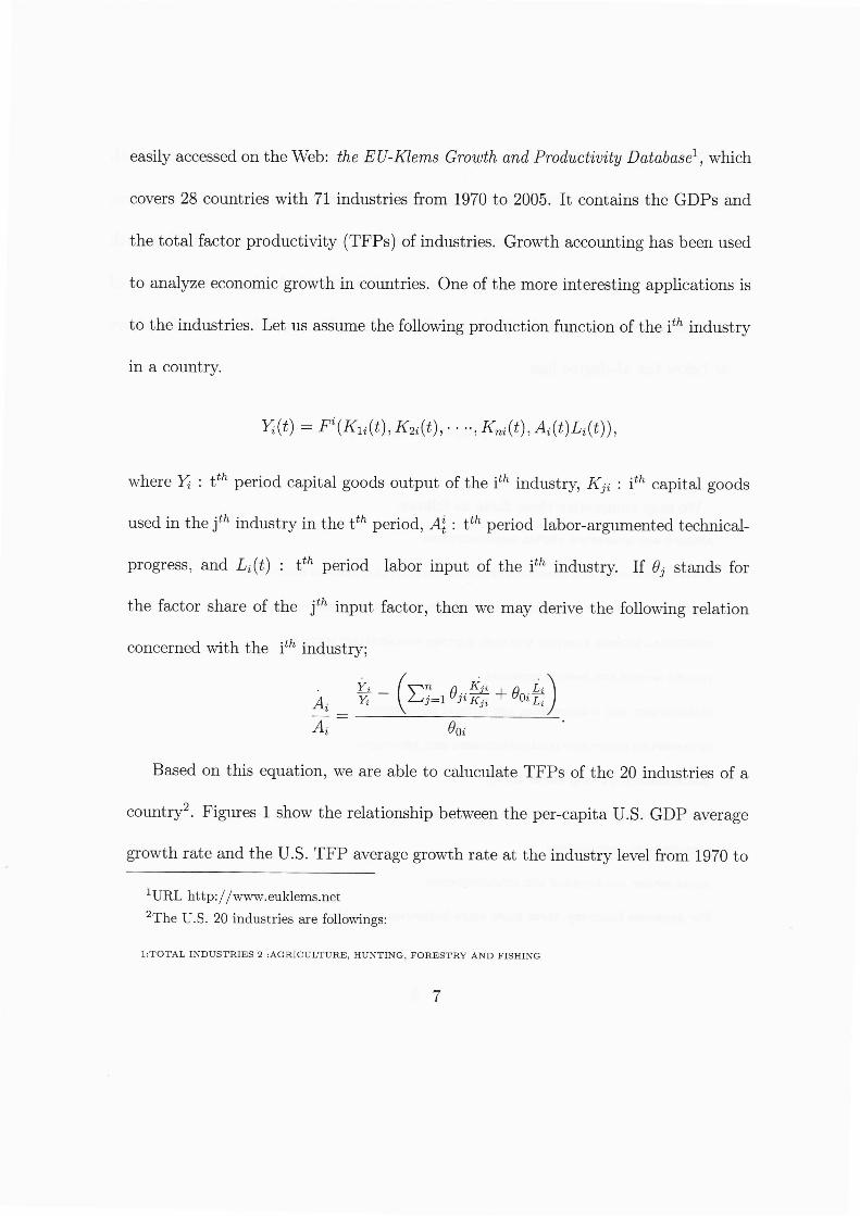
to the industrieso Let us assume the follolving production function of the itんindustry

in a country.

Z(ι)=Fづ(κlじ(t),κ2」(ι),……,κれじ(t),ん(ι)五万(ι)),

where x:ttんperiOd capital goods Output of the itんindustr勇』し :ilんCapital goods

used in the jtんindustry in the ttんperiod,ス::ttんperiod labor¨argumented technical_

progress,and ZJ(ι): ttんperiod labor input of the itんindustry.IfらstandS fOr

the factor share of the jtんinput factor,then we may derive the following relttion

concerned with the itんindustry;

卜1らづ号+θ∝告スづ

Based on this equation,we are able to caluculate TFPs of the 20 industries of a

comtry2.Figures l show the relationship bet■7een the per_capita U.S.GDP average

growth rate and the UoS.TFP average growth rate at the industry level fronl 1970 to

lURL http://、、ヽマW.euklems.net2The U.S.20 industries are foll赫

ngs:

1:TOTAL INDUSTRIES 2:AGRICULTURE,HUNTING,FORESTRY AND FISHING

θOづ

1)Each industrial sector has its oⅥ「n steady state恥′ith the sector speciflc grov7th

rate.

2)The steady state level and its growth rate are highly related to its own TFP.

These facts cannot be explained by the neⅥ r gron/th theory totally based on the

macro production function. Thus、 Ⅳe need to set up an industry based mlllti_sector

gro恥アth model.()n the other hand,the turnpike theory are established based on the

multi―sector model. However it has a drawback, toO. The turnpike theory means

that each industrial sectOr恥アith difFerent initial stocks will eventually converge to its

own optilrnal steady state lⅣith the corllmon balanced gro、、「th rate. In otherヽⅣords,

each industry's per capita stock will cOnverges to a certain constant ratio. Thus the

turnpike theory cannot explaln the facts that each industry's per¨capita stock gro、vs

at its own growth rate,which is determined by the sectoral TFP.

OECD(2003)also Studied the producti宙 ty growth at the industry level in de¨

tail and repOrted the following results, whiぬare consistent with our observations

discussed above.

● A large cOntribution to overall productivity growth patterns comes frolln produc―

tivity changes within industries,rather than as a result of signiflcant shifts Of

emplくら″llnent across industries.

●TFP depends On cOllntry/industry speciflc factors.

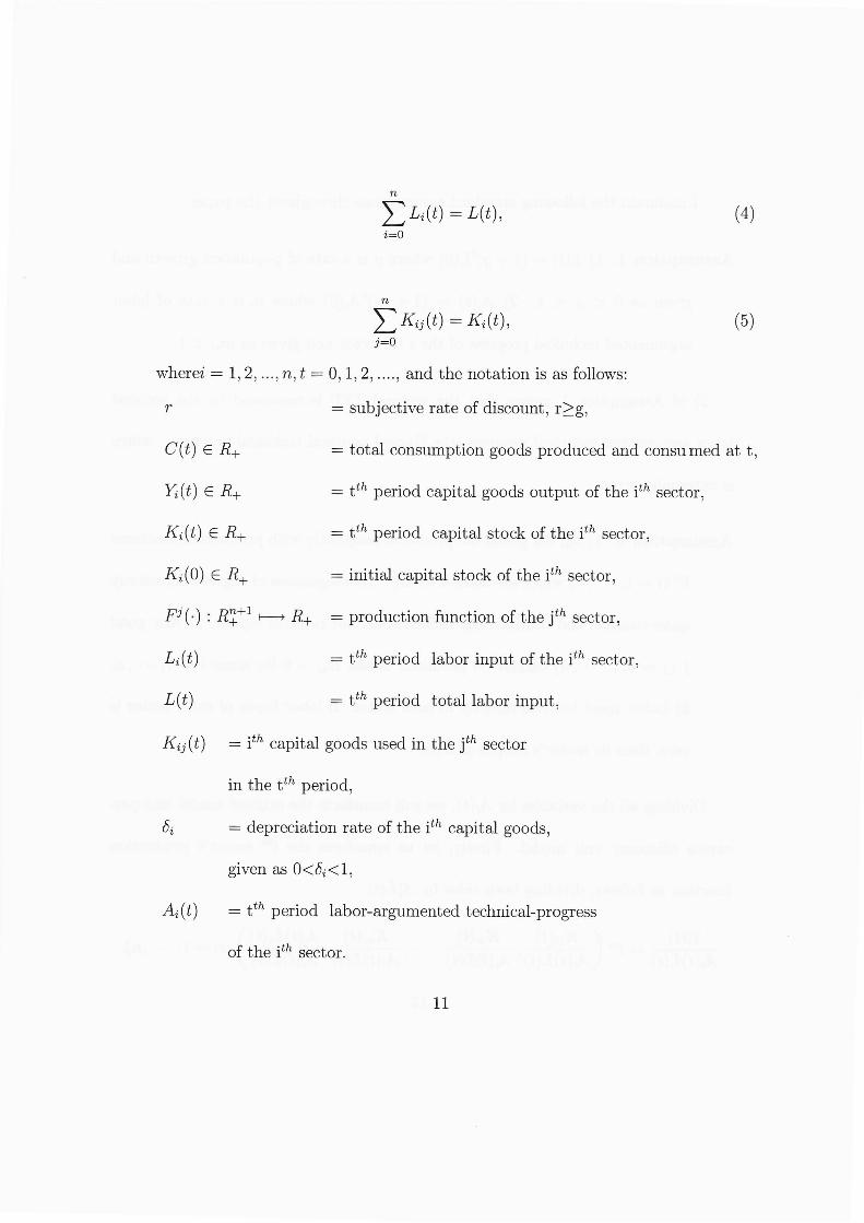
ΣLづ0=LO,づ=0

Σ為0=乙0, 0)′=0

whera=1,2,… ,π,ι=0,1,2,… 。,and the notation is as follows:

r =subjective rtte of discolmt,r≧ g,

σ(ι)∈ R+ =tOtal consllnlption goods produced alld consumed at t,

X(ι)∈ R+ =ttん period capital goods output of the itんsector,

κ (ι)∈ R+ =ttん period capitd stock of the itんsector,

XXO)SR十 =i五 tid capitd stock of the itんsectoL

F賓 。):R#1卜

→ R十 =prOduction function of the jtん seCtOL

Lを(ι) =ttん period lめ or input Of the itんsector,

L(t) =ttん period total labor input,

κり(t)=itん Capitd goods llsed in the jιんsector

in the ttんperiod,

a =depreciation rate of the itんcapital goods,

glven as O<a<1,

スを(ι) =ttん period labor―alrgll■lented tech」cal_progress

of the itんsector.

に)

１■

■■

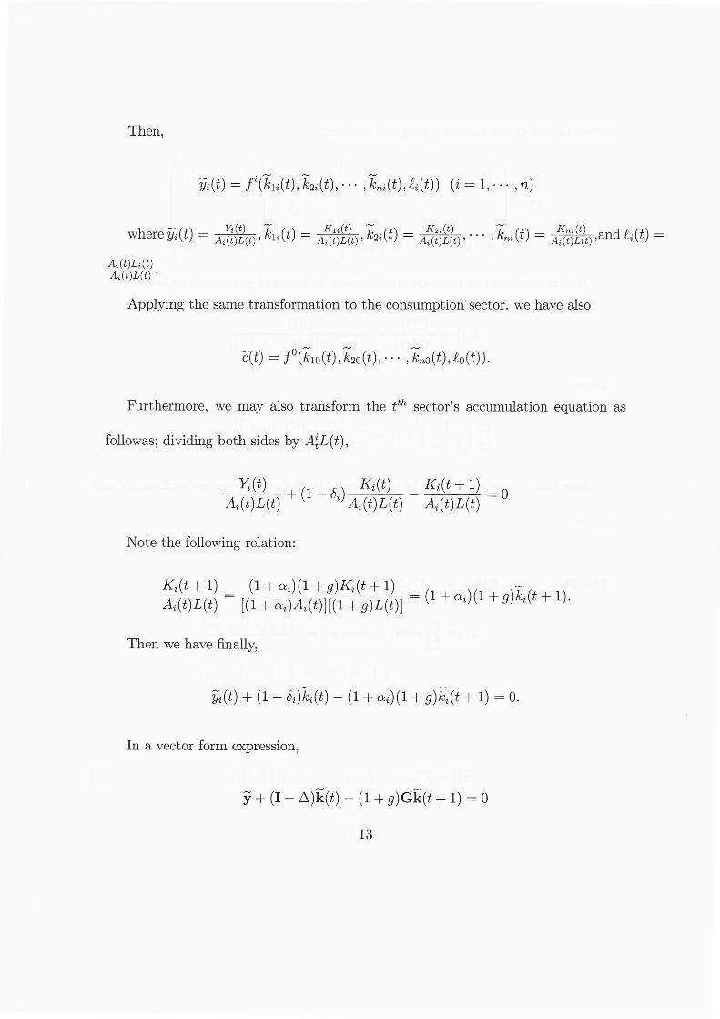
Then,

銑(t)=∫2(た1.(ι),た2づ(t),…・,観を(ι),″づ(ι))(づ=1,…。,η)

where銑(ι)=満 ,πL(ι)=満 ,Lo(ι)=満 ,・・・,Lづ(ι)=ガ譜告,and′。(t)=スt(t)Lt(t)A,(t)L(ι)・

Applying the same transformation to the consumption sector,we have also

ズι)=∫0(πlo(t),LO(ι),・…,Lo(ι),イo(ι)).

Furthermore, we may also transfornl the ttん sector's accumulation equation as

bllowasi dividing both sid∝by 4:L(t),

満‐ ―助

鵜―器

=0

Note the following relation:

器=

瓢 1+0い の歌 科 )

Then we have flnallェ

銑(ι)+(1-a)れ (t)一(1+αを)(1+θ)れ(ι+1)=0.

In a vector forln expression,

テ+(I一△)k(ι)一(1+θ)Gk(ι+1)=0

13

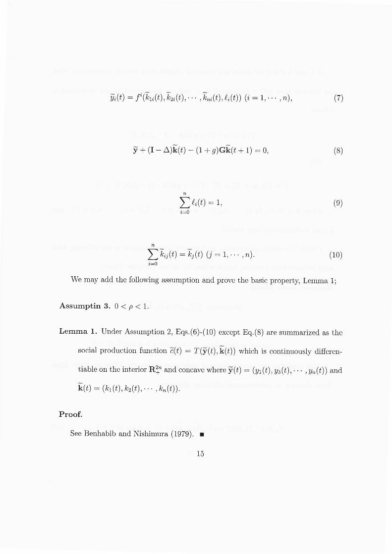
銑(ι)=ノ(■づ(ι),Lづ(ι),…・,Lo(t),″を(ι))(づ=1,…,η),

“

)

テ+(I一 △)k(ι)―(1+g)Gk(ι+1)=0, (8)

Σ″JO=1,`=0

ΣLO=為0。=1,…,け

(9)

( 1 0 )

を=0

We may add the fol10w‐ ing assumption and prove the basic properttt Leln」 Ina l;

ALSSumptin 3. 0<ρ <1.

Lemma l.Under Assumption 2,Eqs。 (6)―(10)except Eq。(8)are summarized as the

social production hnction at)=T(テ(ι),k(t))WhiCh is continuously difFeren―

tiable on the interior Rtt and COncavewhere,(ι)=(νl(ι),御(ι),…,ぃ(ι))and

k(ι)=(た 1(t),た2(ι),…。,たπ(ι)).

Proo■

See Benhabib and NishiIIlllra(1979)。■　

　

５̈１■

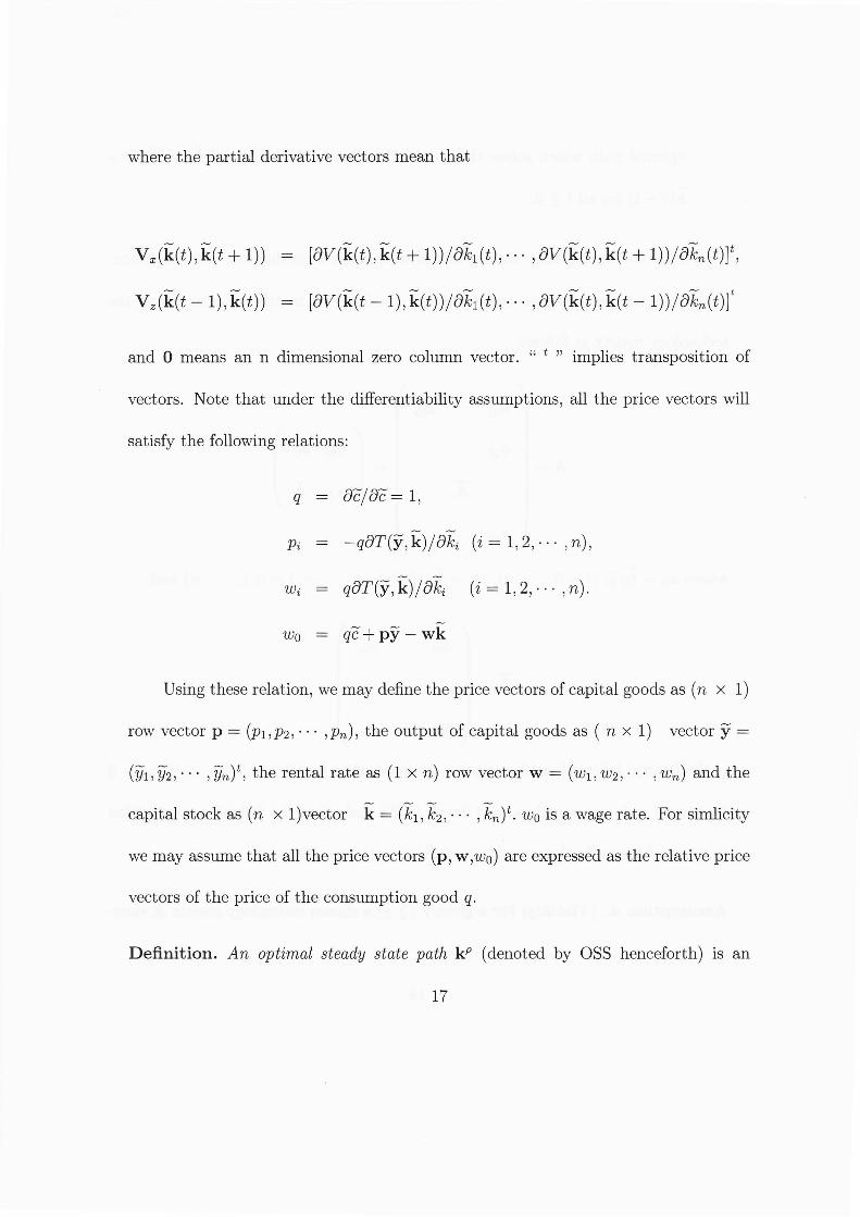
where the partial derivative vectors nleall that

Vω(k(t),k(ι+1))

Vz(k(ι-1),k(ι))

g=町 死 =1,

pづ = -9∂T(y,k)/∂れ

υ` = g∂

T(テ,k)/∂れ

υo=9C tt py― Wk

[∂7(正(ι),正(ι+1))/∂た1(ι),…・,∂y(1(ι),正(ι+1))/∂場(t)]t,

I∂7(1(t-1),I(ι))/∂た1(ι),…。,∂7(1(ι),正(ι_1))/∂たπ(ι)it

and O means all n dilnensional zero coluIIm vector. ``t " ilnplies transposition of

vectors. Note that under the digerentiability assllmptions,all the price vectors恥 アill

satisfy the following relations:

(を=1,2,… ・,η),

(づ=1,2,… ・,η).

Using these relation,we may deine the price vectors of capital goods as(η× 1)

row vector p=(pl,p2,・…,Pπ),the Output of capital goods as(η×1)VeCtOr y=

(■,う,…・,L)t,the rental rate as(1×η)r。、V Vector w=(ωl,ω2,…・,切れ)and the

capital stock as(η ×1)VeCtOr k=(た 1,た2,・… ,たれ)to υo iS a wage rate.For simlicity

we may assume that all the price vectors(p,W,Oo)are eXpressed as the rdative price

vectors of the price of the consumption good g。

Deinition.ス η 9pιづπαJ steααν stαιθ kρ (denoted by OSS henceforth)is an励　　・７

ｐ

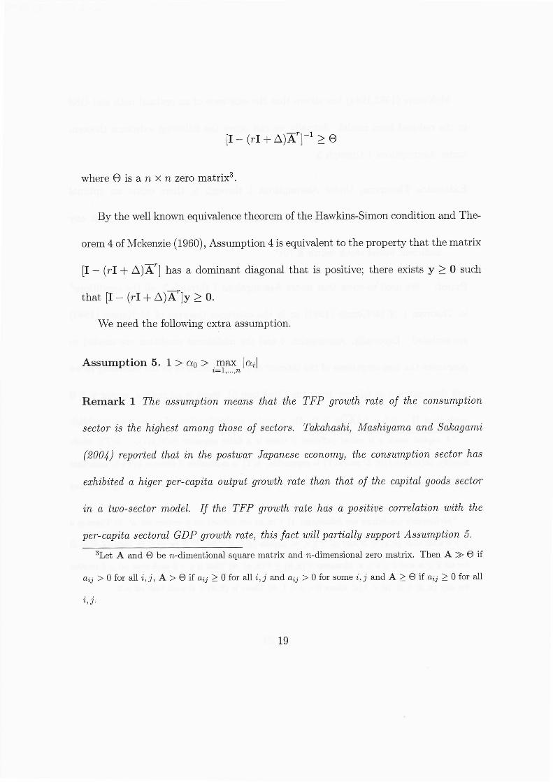
[ I―(rI十△)

where O is a η×η zero matrix3.

コFl~1≧O

By the well known equivalellce theorenl of the Hawkins―Silnon condition and The―

orem 4 of Mckenzie(1960),Assumption 4 is eq■ uvalent to the property that the matr破

「―(rI+△口了]has a dominant diagonal that is positiv%there exists y≧O suCh

that lI一(rI十△フrly≧0.

ヽヽ石e need the following extra assumption.

Assumption 5.1>α O>t当‰ lαじ|

Remark 1 7Lθ αssuηpttθη mθαηs tんαι ιんθ TFP θ"υιん%ιθげιんθ CοηSttηριづοη

secιοr ts ιんθんづgんest αποηg tんοscげsCCtο%.助 たαんαsんを,Mαsんづναπα αηa Sαん

“

απづ

`2θ

θイリ repοrted ιんαι づη ιんθ pοstυαr JOναηcSC ecοηθγnν′ `んθ cοηsttγ,pιづοη scctOrんαS

c仇づbづιθα αんづθer pθttc叩Jια Oυ″υι g“υιん%ιθ ιんαη tんα;げιんθCのりια;gοοαs sectοr

づη α ιυO―sectοr mοαθJ.」/流 θ TFP θttω流 %ιθんαs α PοSをιづυθ cοπじJαιづOη υづιんじんθ

pettcTづια secιο%JG'Pg"υ 仇 %ιθ,ιんじsル ct υづιι Parι`αιJν sTPο rι Ass%π νιづOη」・

3Let」生and O be η―dilnentional squtte matr破and π―dilnensional zero matrix. Then A》>O if

α″>O for a l l t ,ブ,A>Θ if a″≧O for a l lづ,ブand aを′>O for s o m eづ,ブand A≧O if a″≧O fOr a l l

づ,ブ・

19

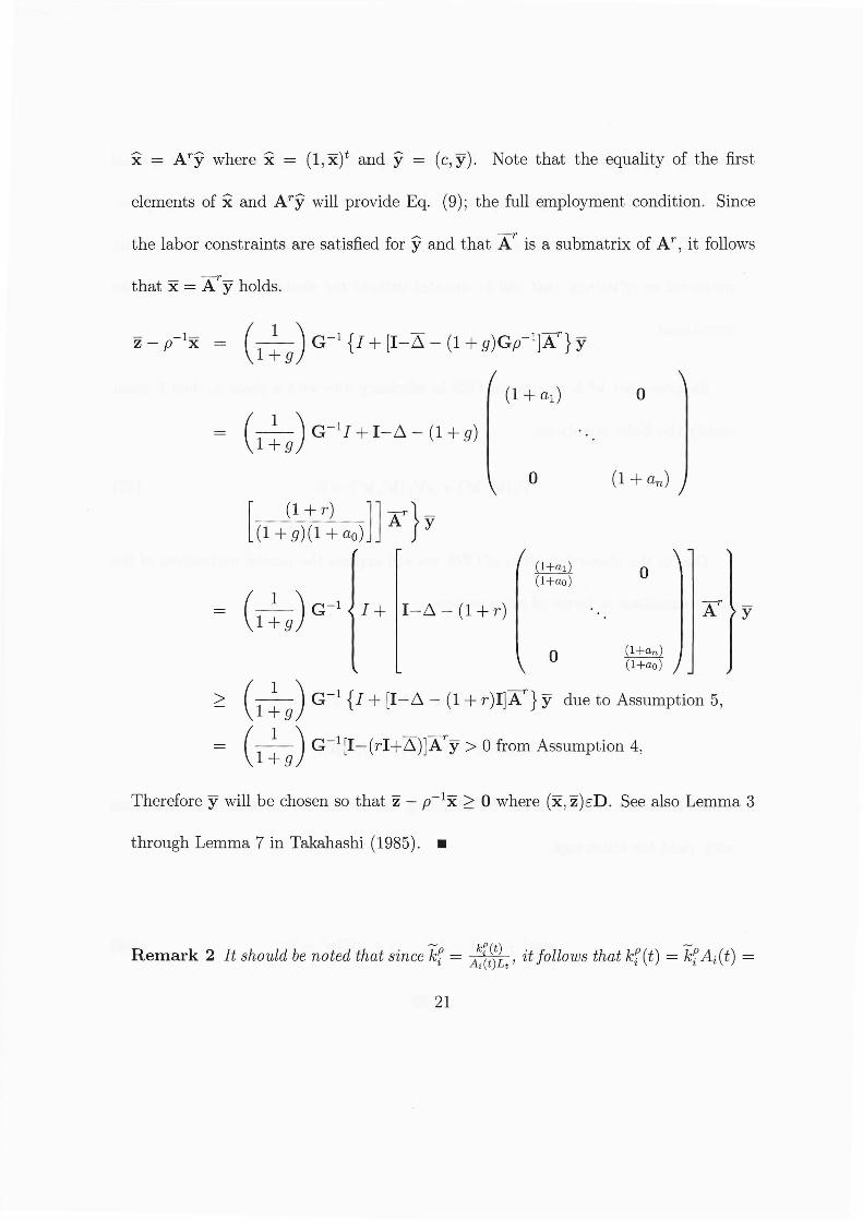
父=Ar,where父=(1,X)t and 9=(c,ア)。Note that the equality of the nrst

elelnents of tt and Ar,will prOvide Eq。(9);the full emplりment conditiono Since

the labor constraints are satisfled for y and that Ar is a submatrix of Jヽr,lt follows

that X=rァ holds.

Z~ρ~lX = (II卜

τ)G~1{」+[I一匹―(1+の Gρ

~11コご}ア

( 1 +α l) 0

0 (1+α れ)

| |1西r}ア

> (島

)G~1{I tt II一

△ ‐―(1+→ IIAr}ァ due tO Assumption 5,

= (T{卜τ)G~lII―

(rI+A)]:瓦Iア>O frOm Assumption 4,

ThereforeァWill be chosen so that Z一ρ~1天

≧O Where(更,7)εDo See also Lerllma 3

through Lelnma 7 in Takahashi(1985)。 ■

Remark 2■ sん鈍Jαろθ ηοιθα ιんαι sれce町 =デ鵞幾 ′づιルJιουS ttαιィ(ι)=町 4。(ι)=

21

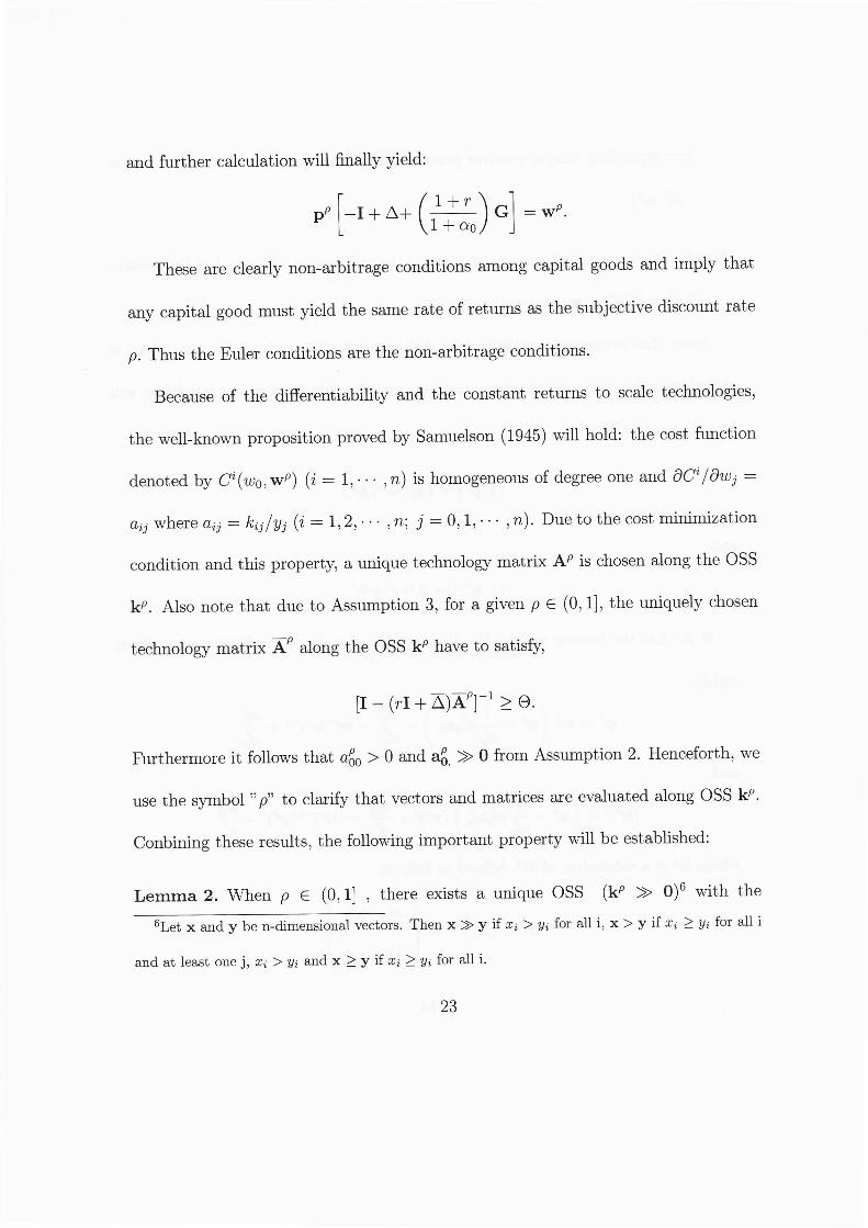
and further calculation will lnally yield:

pρl一I+△+(:≒:」i)GI=wρ.

These are clearly non―鑓bitrage conditions alnong capital goods and imply that

町 capital good must yield the same rate of returns as the subjective discount rate

ρ.Thus the Euler conditions are the non―arbitrage conditions.

Because of the diferentiability and the constant returns to scale technologies,

the well―known proposition proved by Samuelson(1945)will h01d:the cost function

denoted by σ。(oO,Wρ)(づ=1,…。,η)is hOmogeneous of degree one and∂θ」/∂り′=

αづ′where αを」=れ′/坊(づ=1,2,―・,η;ブ=0,1,…。,π).Due to the cost minimizttion

condition and this property,a unique technology matrix Aρ is chosen along the(DSS

kρ.Also n o t e t h a t d u e t o A s s u m p t i o n 3 , f o r a g i v e n ρ∈(0,11,t h e u n i q u e l yぬosen

tec h n o l o g y m a t r i x lρ along t h e O S S r h a v e t o s a t i sサ,

Furthermore it fol lo恥rs that α60>O and a6≫O from Assumption 2.Henceforth,we

use the syllnbol"ρ"to claritt that vectors and matrices are evaluated along OSS kρ.

Conbining these results,the following important property lⅣill be established:

Lemma 2。 When ρ ∈ (0,1,there e対 sts a unique OSS(kρ ≫ 0)6 with the

6Let x and y be n d̈ilrnensional vectors.Then x)>y if πt>ν t for all i,x>y if α`≧

υづfOr all i

a n d a t l e a s t o n e j ,χ乞>νt and x≧y if“J≧υ」for all i .

「―(γI十五)西句~1≧

O。

23

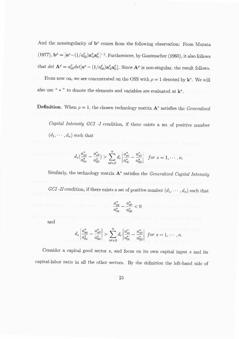
And the nOnsingularity of bρ cOmes fronl the follon・ing observation: Fromヽ411rata

(1977),bρ=[♂―(1/α品)喝ag」-1.FШtth∝mor%by Gantmacher(1960),it dSOおIms

that αθι Aρ=α

“

αθιぽ―(1/α80)喝嘲.].Since Aρ is non…singular,the result follows.

■om now On,we tte concentrated on the OSS with ρ=l denoted by k*.ure宙 11

also use``*''tO denote the elements and variables are e■7aluated at k*.

Deflnition. Vヽhen ρ==1,the chOsen techno10gy matrix A*satisfles the θθηθ?℃あzθご

じ職 り;αJ Lιθηsづり θα ―r cOndition,if there e刈sts a set of positive number

(αl,…・,晩)such that

αs礁一:キ)>鳳島1詣一緒|∫οr s=いちz

Sin■lartt the tettology matr破A*satisies the σθηθ%ιづzθごθ叩づιαJ L`θηsづιν

θar_fr condition,if there exists a set of pOsitive number(αl,…。,απ)suCh that

畿―識<0

and

α31皓―識|>忍銑1詣―皓|∫οr s=い¬牲

Consider a capital good sector s, and fOcus On its own capital input s and its

capital―labOr ratiO in all the other sectors. By the deflnitiOn the left_hand side Of

25

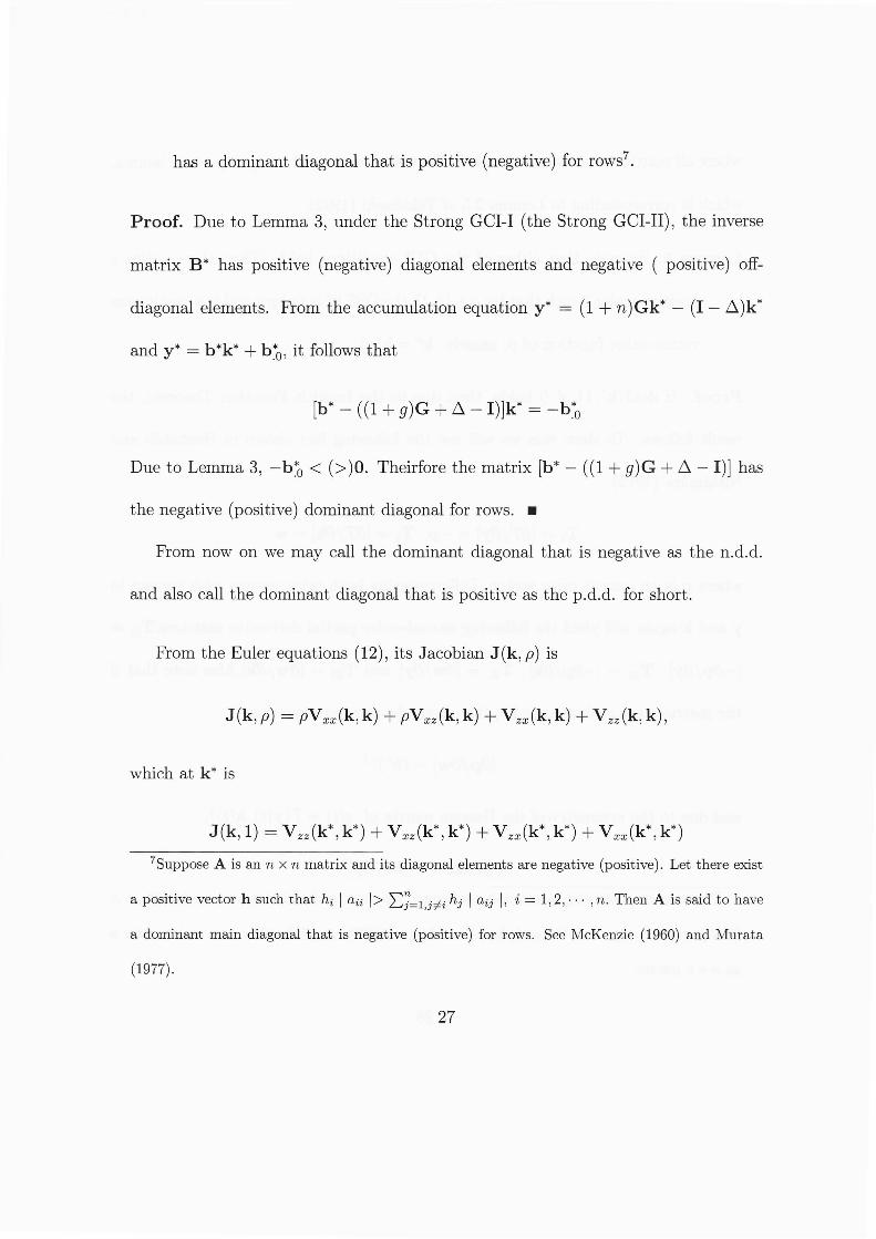
has a dominant diagonal that is positive(negati■7e)おr rOWS7.

Proo■ Due to Lemma 3,under the Strong GCI-1(the strong GCI― Ⅱ),the inverse

matr破 B*has positive(negat市 e)diagOnal delnents and negative(pOSitive)of―

diagonal elements.nЮ m the accumulation equation y*=(1+η )Gk*― (I一△)k*

and y * = b * k *十 bも,it f01 1 0 w s t h a t

[b*一((1+θ)G十△―I)]k*=―bЪ

Dueto Lemma 3,一 bち <(>)0・ Theirfore the matrix[b*一 ((1+g)G+△ 一 I)]has

the negative(positiVe)dominant diagonal for rows.■

■om now on we may call the dollllinant diagonal that is negative as the n.d.d.

and also call the dominant diagonal that is positive as the p.d.d. for short.

■om the Euler equations(12),its」 acobian J(k,ρ )iS

J(k,ρ)=ρ Vπ2(k,k)+ρ Vαz(k,k)+Vz″ (k,k)+Vzz(k,k),

which at k*is

J(k,1)=Vzz(k*,k*)+V“ z(k*,k*)+Vzπ(k*,k*)+V“ω(k*,k*)

7suppOse A is an η×η matrix and its diagonal elements are negative(positiVe).Let there exlst

a positive vector h such thatれlαぅJI>Σ 卜 1,J≠二場 la″ |,づ=1,2,… ,π.Then A is said to hⅣe

a dominant main diagonal that is negative(positiVe)fOr rows.See McKenzie(1960)and Murata

(1977).

27

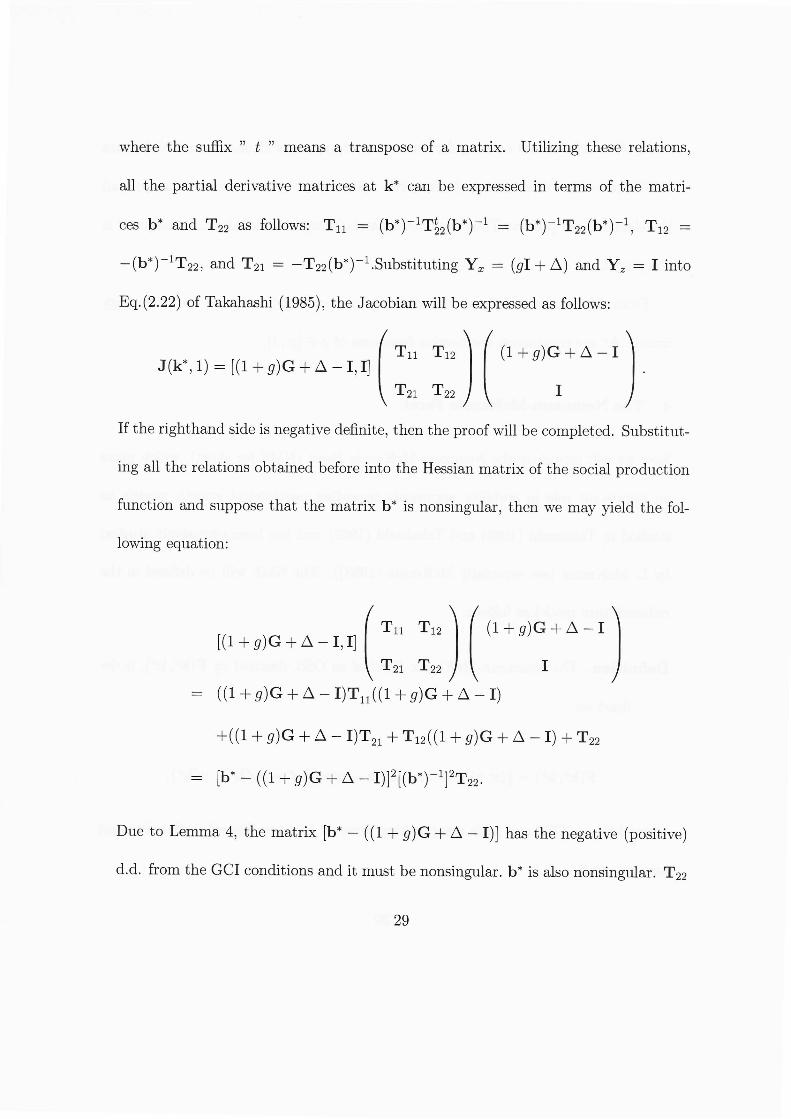
恥′here the sumx " ι '' means a transpose of a matrix. Utilizing these relations,

all the partial derivative matrices at k* can be expressed in terms of the matri―

ces b*and T22 aS f01lows: Tll = (b*)~lT32(b*)~1= (b*)~lT22(b*)~1, T12 =

一(b*)~lT22,and T21=~T22(b*)~1.Substituting Yα=(gI+△ )and Yz=I into

Eq。(2.22)of Takahashi(1985),the」acobian宙1l be expressed as follows:

If the righthand side is negative deflnite,then the proof恥「ill be completed. Substitut¨

ing all the relatiOns obtained before into the Hessian lnatrix of the sOcial production

fllnction and suppose that the lnatrix b*is nonsingular,then we lnay yield the fol―

lom/ing equation:

D u e t o L e m m a 4 , t h e m a t r i x i b *―((1+g)G +△ ―I)]has t h e n e g a t i v e ( p o s i t i V e )

d.d. from the GCI conditions and it lnust be nonsingular.b*is also nonsingular. T22

ヽ

‐

‐

‐

‐

′

ノ

Ｔユ一　

　

　

　

　

　

　

　

　

　

　

　

　

２Ｔ

△

＋

＋　　　　　　　

リヽＩ

Ｇ

　

Ｉ

一

θ　　　　　　　△

＋に

　

　

⊃

　

＋

／‐‐ヽ

「　ｒ　２．

ヽ――ノ塾　切　Ъ

‐　　　　　■■　　　　１́．「Ｊ

Ｔ・２Ｔ２２メＴ・２＜＜け

ｎ

１．

２．

冊

２．＋

哨

Ｔ　　Ｔ　白

／

′

‐

‐

‐

‐

＼

／

１ｌ

　

Ｔ

　

　

一

珂

　

Ｆ　

⊃

　

△

Ｉ　　　≪　　一　　十

一　　　　　　　　　　　　　　　　　　　　　　　　　　　　　　　　　　　　　　　一

轟

＋△．

撚

馘

馘

馘

ぶ

ぃ

ｙ　

　

＋

　　＜

＋　　　十

　

　

１

　

　

一

降

　

鰊　Ｉ　ド

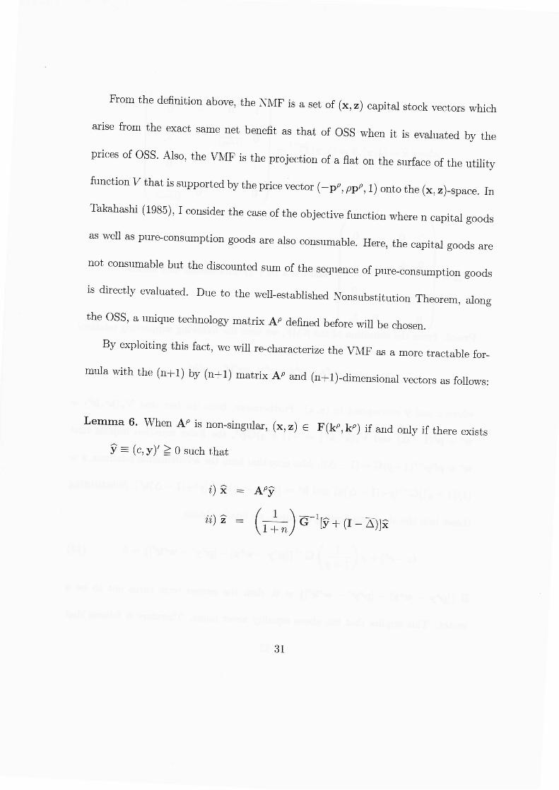
■ om the deinitiOn abOve,the NMF is a set Of(x,Z)capital stOck vectOrs which

atrise from the exact salne net beneit as that Of oss when it is evaluated by the

prices Of osSo AlsO,the VMF is the projectiOn Of a nat on the surface Of the utility

functiOn y that is supported bythe pricettctor(―pρ,ρpρ,1)onto the(x,z)―spaceo ln

Takahashi(1985),I cOnsider the case Of the Objectitt functiOn where n capital goOds

as、Ⅳell as purecOnsumptiOn g00ds are also cOnsumableo Here,the capital goods are

not cOnsurnable but the discOunted suln Of the sequence of pllre_cOnsumptiOn goods

is directly evaluated.Due tO the well_established NOnsubstitutiOn Theorem,along

the(ЭSS,a unique techn010gy lnatrix Aρ deflned befOre恥′ill be chOsen。

By exp10iting this fact,we恥■1l re―characterize the Vル[F as a more tractable fOr―

mula wi t h t h e ( n + 1 ) b y ( n + 1 ) m a t五x Aρ and(n+ 1 )―dimensi O n a l■rectOrs a s f 0 1 1 0 w s :

Lemma 6.ヽ Vhen Aρ is non_singular,(x,z)∈F(kρ,kρ)if and only if there exists

'≡

(C,y)′≧O such that

り父 = Aρ,

02=(∴)。‐p十⊂―到父

31

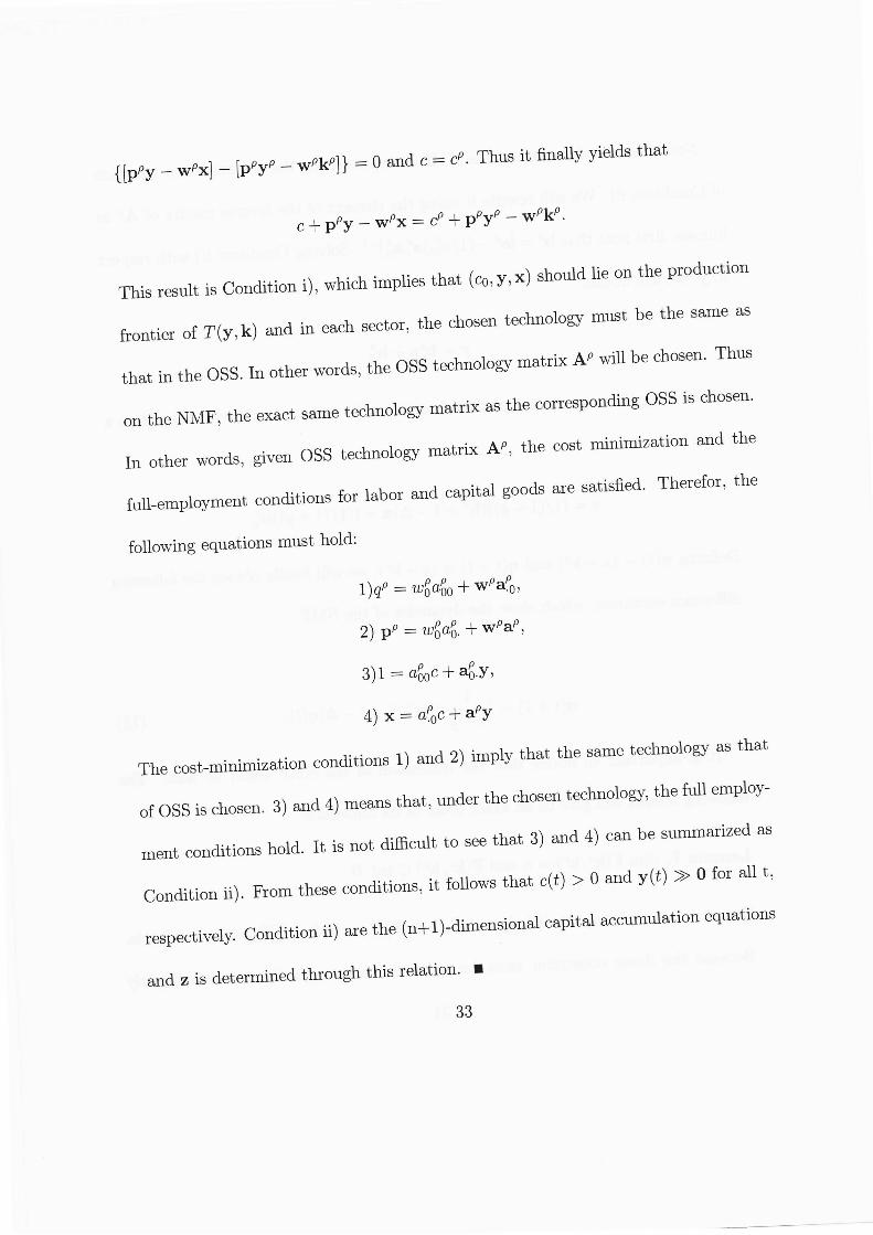
{[pρ

y一‐

Wρ Xl‐―

lpρ

yρ 一‐

Wρ kρl}=O arゞ

C=ぴ 。 「rhus it flnally yiё

ldS that

c+pρy― WρX=Cp+pρ yρ~Wρ kρ・

This reslllt is COndition i),WhiCh implies that(CO,y,X)ShOuld lie on the prOductiOn

士 ontier of T(y,k)and in each SeCtOr,the chOSen techllo10gy lnllSt be the same as

that in the OSS.In Other WOrds,the OSS technology matriX Aρ

win be chosen.Thus

On the NNIF,the eXact same teChno10gy matrix aS the cOrrespOnding(DSS iS ChOSen.

In Other wordS, giVen OSS techn010gy matriX Aρ, the cOSt minilmZation and the

full―employllnellt COnditions for labor and capital goodS are satiSied。

「rherefor,the

fo■owing equationS rnuSt hOld:

1)gρ=り

`α

6o+Wρat,

2)pρ=り6α8・+Wρap,

3)1=α60C十馬y,

4)x=αtC+ry

The COSt―IllllnimiZatiOn conditions l)and 2)imply that the same technology as that

Of OSS iS ChOsen。3)alld 4)meanS that,llnder theぬ

OSen techno10gy,the full emp10y―

ment COnditions hold.It iS not difncult to See that 3)and 4)can be Summarized as

ConditiOn ii).■Om these COnditions,it follo■

vS that C(t)>O and y(t)≫O fOr all t,

respeCt市 elyo COnditiOn ii)are the(n+1)―dimenSiOnal Capital acCumulatiOn equations

alld z iS determined thrOugh thiS relation。■

33

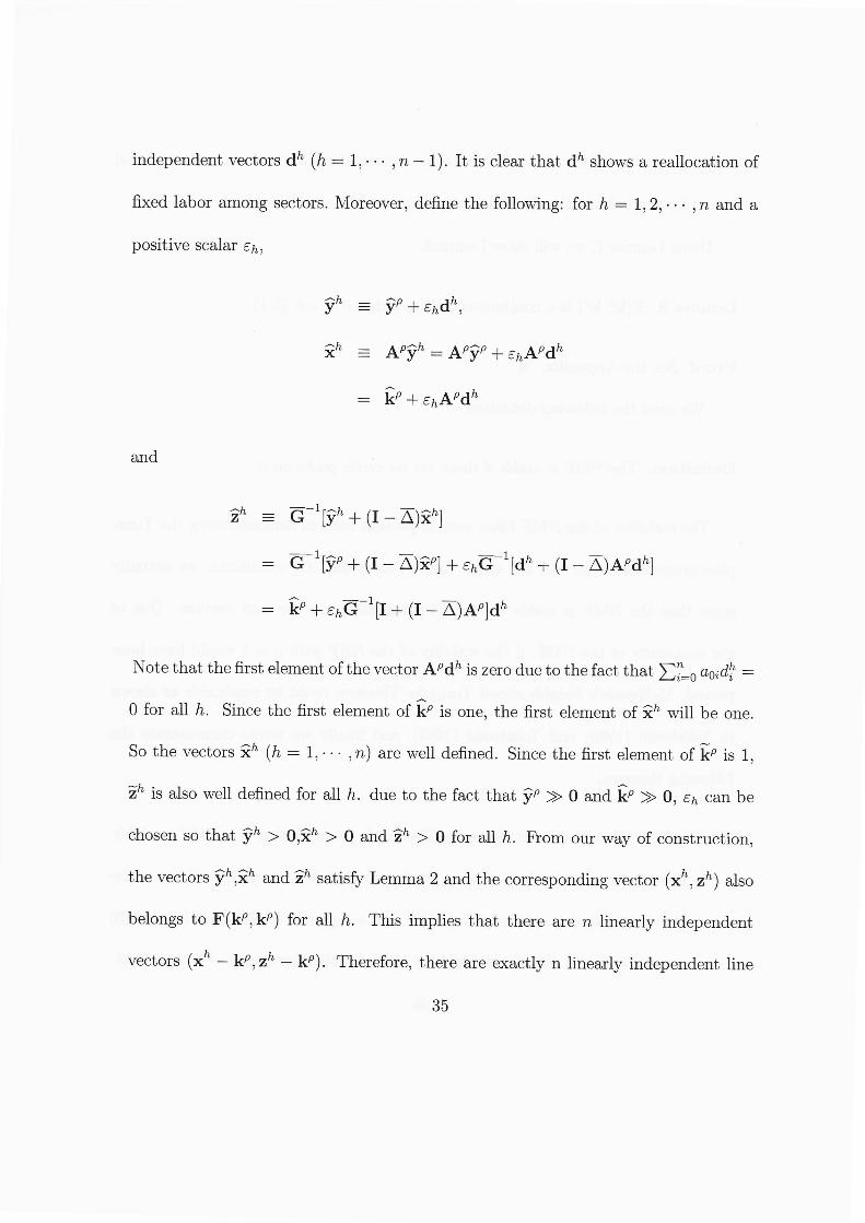
independent vectors dん (ん=1,… 。,η-1)。 It iS Clea that dんshows a rea1location of

flxed labor among sectors.ルlor∞ver,deflne the following: forん=1,2,… ・,η and a

positive scalar εん,

9ρ+εんdん,

Aρ9ん=Aρ,ρ+εんAρdん

シ+εんAρdん

and

〓一　

　

一一一

ん

　

　

　

ん

全ｙ

　　〈Ｘ

″ 三 百~1[9ん

+(I一匹)父句

= C「1[9ρ

+(I― △)父句十εん百~1[dん

+(I一 匹)Aρd句

= 2ρ+εん百~1「

十(I一匹)Attdん

Note that the■rst elemelrlt ofthe vector Aρdんis zero duetothefact that Σ胆O αOを″=

O for allん.Since the■rst element of ttρ is one,the■rst element of父んwill be One.

So the■7ectors父ん(ん=1,・…,η)are well deflnedo Since the nrst element of ttρ is l,

′is alsO well deflned for allん。due to the fact that,ρ≫O and ttρ≫o,εんcan be

chosen so that,ん>0,父ん>o and'>o fOr allん。■om ollr way of construction,

the vectors,ん,父んand"satistt Lemma 2 and the corresponding■/ector(xん,Zん)alSO

belongs to F(P,kρ )fOr allん。This implies that there are n linearly independent

vectors(xん 一kρ,Zん―kρ)・Therefore,there are exactly n linearly independent line

35

Proo■ See the ttgllment of Section 4 of Takahashi(1993)。■

The Neighborhood Turnpike Theoreln lneallls that any optilnal path must be

trapped in a neighborhood of the corresponding OSS and the neighborhood can be

taken as smdl as possible by making ρ close enough to one。

5 1■ lrnpike Theorem

The full Twnpike「 rheoreln is described as the follo、、ring theorenl:

Full Turnpike irheorerrl There is aフ > O C10se enoug to l such that for any

ρ∈腋,1),an optimal path P(ι)宙th the sllmcient initial capital stock will

asymptotically converge to the optimal steady state kρ.

As we ha、 c shown,under Assumption 7, the dilnension of the VNIF is no We

Ⅵrill keep this assumption henceforth. On the other hand,the dynanlics of the Vル IF

is expressed by the n―dimensiond linear dittrellce equation(8).To shOW the full

tllrnpike theorem we need to strengthen the generalized capitl intensity conditionds,

GCI―Iand GCI¨Ⅱ.

Remark 3 ιんθメ“ι`ο bθ ποιθα ttαι jη ιんθ罐万CづθηCν υηづιサC'm,流 θルJJれηPづんθ

πCαηS tんαι θαcんsectοrtt ρpι17ηαι pαιんcοηυθηes tο ιんe οptクηαι steααν stαιθ. fη οttθづηαι

ιθmSげ SerJθs,αην jπα%Sιη b pθttc叩づια CΨjιαJ Stοcんαηα ου″%ιθ"υ

αι ttθ%ιθげ

37

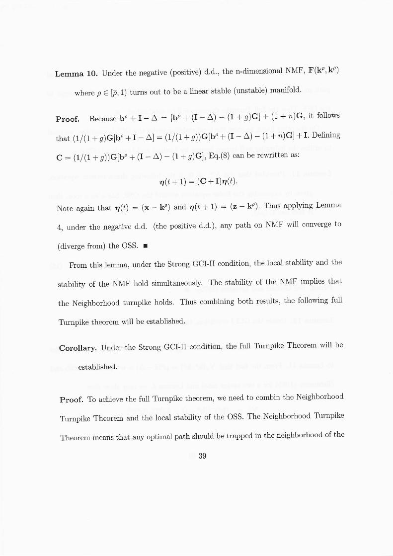
Lemma 10.Under the negat市e(poSitiVe)d.d。,the n―dimensional NMF,F(kρ,r)

where ρ∈レ,1)tllrnS Out tO be a linear stable(lmStable)manif01d・

Proo■ Because bρ +I― △ =[bρ +(I一 △)一 (1+g)G]+(1+η )G,it follows

that(1/(1+g)G[bρ +I― △]=(1/(1+g))Glbρ 十(I―△)― (1+η )G]十 1.Deining

C=(1/(1+g))G[bρ +(I一 △)一 (1+g)Gl,Eq。 (8)can be rewritten as:

η(ι+1)=(C+I)η (ι)・

Note again that η(ι)=(X― kρ)and η(ι+1)=(Z― kρ)・Thus applying Lellnma

4,under the negati(d.d.(the pOSitive d.d。 ),any path on NMF will cowerge to

(d市erge from)the OSS・ ■

Fronl tllis le[llna,under the Strong GCI¨ II condition,the local stability and the

stability of the NⅣIF hold simultaneously.The stability of the NⅣlF implies that

the Neighborhood turnpike holds。 「rhus combillllng both resdts, the following full

Turnpike theorem will be established.

Corollary. Under the Strong GCI¨ II condition,the full Turnpike Theorem ttrill be

established.

Proof. To achieve the full Turnpike theorenl,lⅣ e need to combin the Neighborhood

Turnpike Theorem and the local stability of the(Э SS.The Neighborhood Turnpike

Theorem meanS that any optin■ al path should be trapped in the neighborhood of the

39

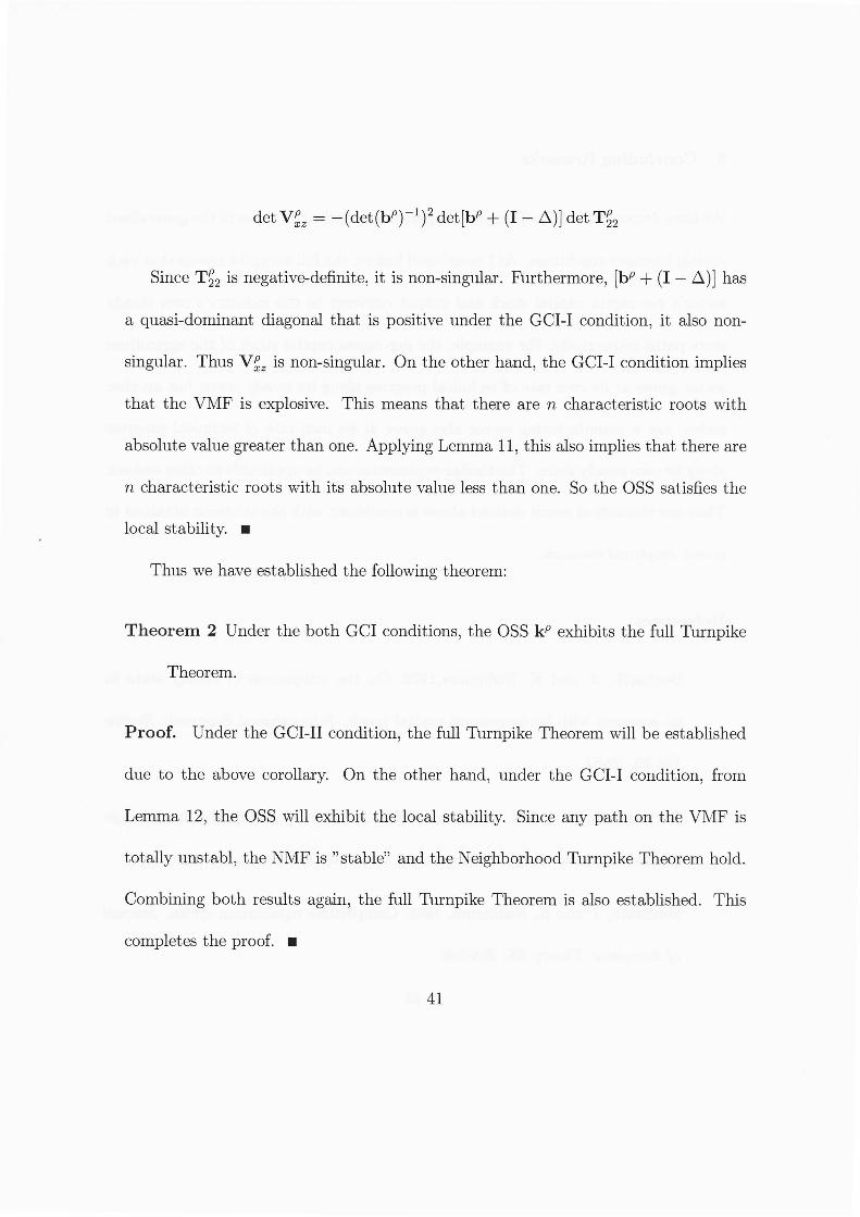
det V`z=―(det(bρ)~1)2 detibρ+(I―△)]detTg2

Since Tg2 iS negat市e―deinite,it is non―singular.Furthermore,[bρ+(I―△)]has

a quasi―donlinant diagonal that is positive under the GCI―I condition,it also non―

singlllaro Thus Vgz is non_singular。On the other hand,the GCI―I condition inlplies

that the VNIIF is explosive. This means that there are n characteristic roots恥 ■th

absolute value greater than one.Applying LeIIma ll,this also implies that there are

n characteristic roots with its absolute■7alue less than one. So the OSS satisfles the

local stability.■

Thus we have established the fo1lo、、ring theorenl:

Theorem 2 Under the both GCI conditions,the(DSS kρ exhibits the full Turnpike

Theoreln.

Proo■ Under the GCI― II condition,the full Turnpike Theorem will be established

due to the above corollary. On the other hand, under the GCI… I condition, from

Lelrlma 12,the OSS will exhibit the local stability.Since any path on the VⅣ IF is

totally unstabl,the]ヽA/1F is''stable''and the Neighborhood TШ npike irheorelllll h01d.

Combining both results again,the full「 Furnpike rrheorem is also established. This

completes the proof。 ■

41

Benhabib,J.嗣 A.Rustichini,1990。 Eqllihbriuln cycling with sman discount¨

ing.力 鶴rηα:げ Ecοποπ'C rLcoη

52,423-432.

Burmeister,E.and A.Dobell,1970.Mα ιんθπα

“

cαJ=んθοη げ ECοποπづCσ"υ

カ

仲IaCmillan,London)。

Bllrnleister,E.and]Do Grahnl,1975.Price expectations and global stability in

economic systems.■ υιOπαι,cα ll,487-497.

Gantmacher,F.」θδθ.動 θTんθοη げ ναιttces υοJ.1(Chelsea,New York)。

Inada,K. 1971.The production coemcient inatrix and the Stolper― Samuelson

condition.Ecοηοπθ力巧cα 39,88-93.

Jones,R。,S.Ⅳlariit alld To Mitra,1993.The Stolper―Samudson theoreln:Links

to dollninant diagonals,in: R.Becker,Wl.Boldrin,R.Jones and W.Thomson,

eds。,σθηθ%J Egυづιりb西しπ,G"υ tt αηα 7勉αθ〃 ―ιんθ Jηαcνげ五`οπθJ McκcηZθ,

(Academic Press,San Diego).

Levhari,lD.and No Liviatan,1972.On stability in the saddl()point sense.JOur―

ηα;げ ECοηοmづc ttθο町 4,88-93.

Lucas,R"1988.A Mechanics of Economic Dewlopment.力υttαJげ MοηCιαη

Ecοηοηιtcs 22,3 4̈2.

43

Scheinkman,J。,1976。An optilnal steady state of n―sector growth model when

utility is discounted.力%鶴αJげEcοηοmづc ttθοり 12,11…20.

Romer,P。 ,1986.IК reasing Retllrns and Lomg― rlln growth.力 し物αιげ Pο」づι'Cα

ι

Ecοηοπν 94,1002-1037.

Srini■7asan,T。,1964.Optilnal savings in a two―sector lnodel of growth.Ecοηο―

πθ`西

cα 32,358-373.

Takahashi, H., 1985.Cん α%cιθれzαιづοηsげ Oρι`mα

ι P"gmmsづ η J可2ηJιθ

Ecοποmづes,Ph.Do Dissertation,the University of Rochester.

Takahashi,H.,1992.The von Neumann facet and a global asymptotic stability.

五ηttαゐげOρθ%ιりοηs Resθαにん37,273…282.

Takahashi,H.,2001.A stable optimal cycle with small discounting in a two―

sector discretetilne model。∫彎 αηesc Ecοηοπづc RθυJcυ 52,Ar。.ュ θ2θ―θθ∂・

Takahashi,H。,Ko Mashiyama,To Sakagallni,2009。Why did Japan grow so fast

dllring 1955…1973 and the Era of High…speed Growth end after the Oil―shock?:

ⅣIeasuring capital intensity in the postwar」apanese econo、 、Working Paper

08-2,Dept.of Economics,Metti Gakuin U五 versity.

Yano,M。 ,1990。Von Nellmann facets alld the dynallnic stability of perfect fore

45

F(k(ρ′))Where(xr,Z′ )∈

jηt D,(x,z)≠ (X′,Z′)alld ρ′∈ レ ,1)iS ChOSen close enough

to ρ.Now let us deine the plain Hα is deflned as fo1lov/s:

Hα≡{(X,Z)CD:ιolαk(ρ′)十(1-α)k(ρ),αk(ρ

′)+(1-α)k(ρ)]+

ππ

Σtんぽ7)+(1-→ガlpl,αノr)+(1-→Z′lpll}りんere Σιん=1・ん=1ん=1

We can dways ind an intersection(xα ,Zα)betWeen Hα and the line obt温ned by

collnecting points(x,Z)alld(X′ ,Z′)llnless(x,z)=(Xr,Z′ )。 Since(Xα ,Zα )iS On the

plain Hα,it can also be expressed as follows:

(Xα,Zα)=ι8[αk(ρ′)十(1-α)k(ρ),αk(ρ

′)十(1-α)k(ρ)]+

π

ΣιЯbガ。つ+(1-→X′0),αノ0つ十(1-→Z′0レんere ΣιЯ=1・ん=1ん=1

where α―→0,レk(〆)+(1-α)k(ρ)]―→k(ρ)andレXん(ρ′)+(1-α )Xん(ρ),αZん(ρ′)+

(1-α )Zん(ρ)]→ (Xρ,Zρ)fOrん=1,… ・,η.Therefore(xα ,zα)COmに rges to(x,Z)as

α→ 0.Also n o t e t h a t ( xα,Zα)∈づηι D due t o t h e c o n、rexity o f D a n d t h e f a c t t h a t

(X′,Z7)∈づηι D・On the other hand,because of the continuity of k(ρ),X(ρ)alld Z(ρ)

in ρ∈腋,1)。fOr any εα>O there e対 sts δα>O such that lρ

α―ρl<δα implies that

‖k(ρα)一[αk(〆)+(1-α)k(ρ)]‖<ε

α

alld forん=1,… 。,η,

| | ( k (ρα),k(ρα))一IαXん(ρ′)+(1-α)Xん(ρ),αZん(ρ

′)+(1-α)Zん(ρ)]‖<εα

47

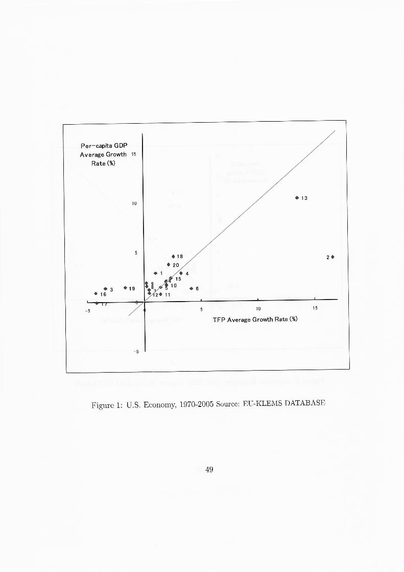
Per―capFta GDP

Average Growth 15

Rate(%)

● 18

◆ 20

◆ 4

15

10

10

T F P A v e r a g e G r o w t h R a t e ( % )

Figure l:U.S.Economy,1970-2005 Source:EU― KLEWIS DATABASE

49