Int. J. Appl. Math. Comput. Sci., 2013, Vol. 23, No. 2, 357–372DOI: 10.2478/amcs-2013-0027

AN UNCONDITIONALLY STABLE NONSTANDARD FINITE DIFFERENCEMETHOD APPLIED TO A MATHEMATICAL MODEL OF HIV INFECTION

HASIM A. OBAID ∗ , RACHID OUIFKI ∗∗, KAILASH C. PATIDAR ∗∗∗

∗ Department of Mathematics and Applied MathematicsUniversity of the Western Cape, Bellville 7535, South Africa

∗∗DST/NRF Centre of Excellence in Epidemiological Modelling and AnalysisStellenbosch University, Stellenbosch 7600, South Africa

∗∗∗Department of Mathematics and Applied MathematicsUniversity of the Western Cape, Private Bag X17, Bellville 7535, South Africa

e-mail: kpatidar@uwc.ac.za

We formulate and analyze an unconditionally stable nonstandard finite difference method for a mathematical model of HIVtransmission dynamics. The dynamics of this model are studied using the qualitative theory of dynamical systems. Thesequalitative features of the continuous model are preserved by the numerical method that we propose in this paper. Thismethod also preserves the positivity of the solution, which is one of the essential requirements when modeling epidemicdiseases. Robust numerical results confirming theoretical investigations are provided. Comparisons are also made with theother conventional approaches that are routinely used for such problems.

Keywords: HIV infection, dynamical systems, nonstandard finite difference methods, equilibria, stability.

1. Introduction

Mathematical models play a significant role inunderstanding the dynamics of biological systems.In most cases, these models are described by autonomoussystems of nonlinear ordinary differential equations,(see, for example, the works of Kouche and Ainseba(2010), Xu et al. (2011), and the references therein).Very often, such systems are so complex that their exactsolutions are not obtainable and hence the need for robustnumerical methods arises. However, as mentioned byVillanueva et al. (2008), numerical methods like thoseof Euler, Runge–Kutta and others fail to solve nonlinearsystems generating oscillations, chaos, and false steadystates. One way to avoid such numerical instabilitiesis the construction of nonstandard finite differenceschemes. Dimitrov and Kojouharov (2007) pointedout that numerical methods one uses to approximatethe solutions of dynamical systems are expected to beconsistent with the original differential systems, andshould be zero-stable and convergent.

In view of the above, in this paper we design a specialclass of numerical methods, known as NonStandard

Finite Difference Methods (NSFDMs). These NSFDMsare explored by many researchers to solve problems inbiological sciences and other areas. Below, we mentiona few of them.

Arenas et al. (2008) developed a nonstandardnumerical scheme for an SIR (where S, I and R standfor susceptible, infected and removed individuals,respectively) seasonal epidemiological model forRespiratory Syncytial Virus (RSV). They compared theirtechnique with some well-known explicit methods andcarried out some simulations with data from Gambia andFinland. They showed that the forward Euler and fourthorder Runge–Kutta schemes do not converge unless thestep-size used in the numerical simulations for these twomethods is less than a critical step-size hc = 0.1.

Some useful studies on dynamical systems arethose by found in the works of Duleba (2004), Rauhet al., (2009; 2009), as well as Zhai and Michel(2004). General two-dimensional autonomous dynamicalsystems and their standard numerical discretizations areconsidered by Dimitrov and Kojouharov (2005) whodesigned and analyzed nonstandard stability-preserving

358 H.A. Obaid et al.

finite-difference schemes based on the explicit andimplicit Euler and the second-order Runge-Kuttamethods. The methods proposed in that paper canbe applicable for solving arbitrary two-dimensionalautonomous dynamical systems. In another work,Dimitrov and Kojouharov (2006), formulated positive andelementary stable nonstandard finite-difference methodsto solve a general class of Rosenzweig–MacArthurpredator-prey systems which involve a logistic intrinsicgrowth of the prey population. Their methods preserve thepositivity of solutions and the stability of the equilibria forarbitrary step-sizes, while the approximations obtainedby the other numerical methods experience difficultiesin preserving either the stability or the positivity of thesolutions, or both.

Gumel et al. (2005) investigated a class of NSFDMsfor solving systems of differential equations arising inmathematical biology. They showed that their methodscan often give numerical results that are asymptoticallyconsistent with those of the corresponding continuousmodel by using a number of case studies in humanepidemiology and ecology.

Some fundamental concepts and applications ofnonstandard finite difference schemes for the solution ofan initial value problem of ordinary differential equationsare presented by Ibijola et al. (2008). They stated thereason why nonstandard methods are needed despite thefact that we have numerous standard methods availableby pointing out that one of the shortcomings of standardmethods is that qualitative properties of the exact solutionare not usually transferred to the numerical solution.

Jódar et al. (2008) explained how to constructtwo competitive implicit finite difference schemes fora deterministic mathematical model associated withthe evolution of influenza in human population. Theyobtained numerical simulations with different sets ofinitial conditions, parameter values, and time step-sizes.

Villanueva et al. (2008) developed (and analyzednumerically) nonstandard finite difference schemes whichare free of numerical instabilities, to obtain the numericalsolution of a mathematical model of infant obesitywith constant population size. This model consists ofa system of coupled nonlinear ordinary differentialequations describing the dynamics of overweight andobese populations. The numerical results presented in thatpaper showed that their methods have better convergenceproperties when compared to the classical Euler or thefourth-order Runge–Kutta methods and the MATLABroutines in the sense that these routines give negativevalues for some of the state variables.

The relationship between a continuous dynamicalsystem and numerical methods to solve it, viewed asdiscrete dynamical systems, is studied by Anguelov et al.(2009). In this work, the authors further categorized theterm ‘dynamic consistency’ as the ‘topological dynamic

consistency’ and proposed a topologically dynamicallyconsistent nonstandard finite difference method.

Applications of these NSFDMs for singularlyperturbed problems can be seen in the work of Kadalbajooet al. (2006), Lubuma and Patidar (2006; 2007c; 2007a;2007b), Munyakazi and Patidar (2010), Patidar andSharma (2006a; 2006b), or Patidar (2008). However, anexhaustive account of work that use such methods isprovided in the survey article by Patidar (2005).

In this paper, we consider a mathematical modelof HIV infection proposed by Bacaer et al. (2008).The governing model is an initial value problem for asystem of nonlinear ordinary differential equations. Itdescribes the dynamics of HIV epidemic by partitionof human population into susceptibles and infectioussubpopulations, denoted respectively by S and I . Wemodify this model by incorporating a function of theHill type for the transmission rate of HIV rather than thefunction e−λH used by Bacaer et al. (2008), where λ isa parameter representing the behavioral change and Hdenotes the HIV prevalence.

We develop some NSFDMs for numerical solutionof a nonlinear system of ordinary differential equationsdescribing the transmission dynamics of HIV. To thebest of our knowledge, this is the first time that theseNSFDMs are designed for this system. To keep themethods fully explicit, we will use the forward differenceapproximations for the first derivative terms. The nonlocalapproximations will be used to tackle the nonlinear terms.In some cases, we will also make use of denominatorfunctions which are a little more complex functions of thetime step-size than the classical one. Furthermore, we willshow that these NSFDMs preserve some key properties ofthe corresponding continuous model. It should be notedthat the proposed schemes are unconditionally stable.

The rest of this paper is organized as follows.The continuous model and its stability properties arediscussed in Section 2. In Section 3 we design andanalyze a numerical method to solve the model proposedin Section 2. Further numerical analyses as well as somenumerical simulations are presented in Section 4. Athorough discussion on the results as well as the scopefor some future research is presented in Section 5.

2. Mathematical model

In this paper, we will consider the mathematical model forHIV proposed by Bacaer et al. (2008) that describes thedynamics of HIV epidemic. The total human populationis divided into susceptibles and infectious subpopulationsdenoted by S and I , respectively. It is assumed that,at any time t, new recruits enter the susceptible classat a constant rate B. Upon effective contact with aninfectious individual at time t, a susceptible individualacquires infection and moves into the class I of infectious

An unconditionally stable nonstandard finite difference method. . . 359

Table 1. Description and values of parameters used in the sys-tem (1).

Description Parameter Value

Birth rate B 200/yearMaximum transmission rate d 0.7/yearParameter representing λ0 5.9behavior changeNatural death rate μ1 0.02/yearMortality rate of infectious μ2 0.1/yearindividualsHill coefficient k variable

individuals. The effective contact rate at time t is denotedby f(H(t)). It is a decreasing function of the HIVprevalence H that reflects a reduction in risky behaviorresulting from the awareness of individuals to a higherHIV prevalence. The death rates of susceptible andinfected individuals are respectively denoted by μ1 andμ2. Using these notations and terminology, the governingmodel is described by the following nonlinear system ofordinary differential equations:

dS(t)dt

= B − f(H(t))H(t)S(t) − μ1S(t),

dI(t)dt

= f(H(t))H(t)S(t) − μ2I(t),(1)

where H(t) is the prevalence of HIV given by

H(t) =I(t)N(t)

, (2)

withN(t) = S(t)+I(t) as the total number of population.The function f(H) in this model is considered to be

the following function of the Hill type:

f(H) =d

1 + λ0Hk, k ≥ 1, (3)

where d, λ0 and k are real numbers and defined inTable 1. The descriptions of the state variables and othertime-invariant parameters as well as their values (aspresented by Bacaer et al. (2008)) are given in Table 1below.

Remark 1. It should be noted that the model (1) does notdistinguish the progression stages of HIV infection. Theaim of this work is to focus on the impact of the responsefunction on the dynamics of the model where estimates ofthe parameters are considered averages over all stages asindicated by Bacaer et al. (2008). However, regarding thestage progression property, the readers may refer to thework of Gumel et al. (2006) and the references therein.

The following results, which determine the basicqualitative features of the continuous model (1), willbe useful in designing a robust nonstandard finite

difference method for solving (1). These results (whichare easy to prove) will further be used in measuring thecompetitiveness of NSFDMs.

Theorem 1. The set

D ={

(S, I) ∈ R2+ : S + I ≤ B

μ1

}

is positivity-invariant for the system (1).

The basic reproduction number of the system (1) isgiven by

R0 =d

μ2. (4)

To find the equilibria of system (1), we notice that, interms of the prevalence of HIV at an equilibrium

H∗ =I∗

S∗ + I∗,

the system (1) has the following characteristic equation:

H∗(μ2λ0H∗k + dH∗ + μ2(1 −R0)) = 0, (5)

whereH∗ = 0 corresponds to the disease free equilibrium

E∗0 =

(B

μ1, 0), (6)

and any (as we can have more, one for each H∗) endemicequilibrium is given by

E∗ =(

B(1 −H∗)μ1(1 −H∗) + μ2H∗ ,

BH∗

μ1(1 −H∗) + μ2H∗

),

(7)where H∗ is a positive solution of the equation

μ2λ0H∗k + dH∗ + μ2(1 −R0) = 0. (8)

However, the above endemic equilibrium will beunique if R0 > 1. (Note that, in this case, the functiondefined by Eqn. (8) is increasing, which means that thereis only one endemic equilibrium point.) In summary,

• if R0 ≤ 1, then only the disease free equilibriumexists;

• if R0 > 1, then there exists a unique endemicequilibrium.

As a consequence of the above results, we have thefollowing theorem.

Theorem 2. For any value of the Hill coefficient k, thesystem (1) exhibits a transcritical bifurcation.

360 H.A. Obaid et al.

Now, for k = 1, we provide the equilibria andtheir basic stability properties for the system (1). Whilethe disease free equilibrium is given by (6), the uniqueendemic equilibrium of this system reads as

E∗ = (E∗1 , E

∗2 ) , (9)

which exists only if R0 > 1, where

E∗1 =

B(1 + λ0)μ1(1 + λ0) + μ2(R0 − 1)

E∗2 =

B (R0 − 1)μ1(1 + λ0) + μ2 (R0 − 1)

.

It can further be proved that these equilibria have thefollowing stability properties:

Theorem 3. The disease free equilibrium of the sys-tem (1), E∗

0 , is locally asymptotically stable if R0 < 1and unstable if R0 > 1.

Theorem 4. The disease free equilibrium of the sys-tem (1), E∗

0 , is globally asymptotically stable in D ifR0 < 1.

Theorem 5. The endemic equilibrium of the system (1),E∗

1 , is locally asymptotically stable if R0 > 1.

Regarding the cases when k > 1, it can be seen from(8) that the analytical evaluation of equilibria becomesalgebraically cumbersome. We therefore evaluate themnumerically, and we will also investigate some of theproperties that they possess. This will be done inSection 4.1.

3. Construction and analysis of the NSFDM

In this section, we design a nonstandard finite differencemethod that satisfies the positivity of the state variablesinvolved in the system. It is important that a numericalmethod preserves this property when used to solvedifferential models arising in population biology becausethese state variables represent subpopulations which nevertake negative values.

To begin with, the time domain [0, T ] is partitionedthrough the discrete time levels tn = n�, where � > 0 isthe time step-size.

To construct the NSFDM, we discretized thesystem (1) based on the approximation of the temporalderivatives by a generalized first order forward differencemethod as follows.

For S(t) ∈ C1(R), the discrete derivative is defined

by

dS(t)dt

=S(t+ �) − S(t)

ψ(�)+ O(ψ(�)) as �→ 0, (10)

where ψ(�) is a denominator function (Mickens andSmith, 1990; 2007) which is a real-valued function andsatisfies

ψ(�) = �+ O(�2) for all � > 0. (11)

The discrete derivative for I(t) is obtained analogouslywhereas the non-derivative terms are approximatedlocally, i.e., at the base time level.

Denoting the approximations of S(nh) and I(nh)by Sn and In, respectively, where n = 0, 1, 2, . . . , theNSFDM reads

Sn+1 − Sn

ψ(�)= B − μ1S

n+1 − f(Hn)HnSn+1,

In+1 − In

ψ(�)= f(Hn)HnSn+1 − μ2I

n+1,

(12)

where discretizations for H and f(H) are given by

Hn =In

Sn + In(13)

and

f(Hn) =d

1 + λ0(Hn)k, (14)

respectively.

Remark 2. It is to be noted that, besides the useof a non-classical denominator function, we have alsoused some non-local discretizations. As mentioned inthe literature (see, e.g., Mickens and Ramadhani, 1994;Patidar, 2005) a finite difference method is termed anonstandard finite difference method if either we use adenominator function or a non-local approximation. Inview of this, when ψ(�) = �, the above method will bereferred to as “NSFDM-I”. However, if the denominatorfunction ψ(�) is different from �, the method will bereferred to as “NSFDM-II”. In this work, this function isconsidered to be (eμ2� − 1)/μ1, μ2 > μ1.

Simplifying (12), we obtain

Sn+1 =Sn + ψ(�)B

1 + ψ(�) {f(Hn)Hn + μ1} ,

In+1 =In + ψ(�)f(Hn)HnSn+1

1 + μ2ψ(�).

(15)

The positivity of the solution reflects from the abovemethod (15), because if the initial values S(0) and I(0)are non-negative then the right hand side of (15) admitsno negative terms for any of n = 0, 1, 2, 3, . . . .

In the following section we determine the stabilityproperties of the system (12), and we verify that

(i) the continuous and the discrete models have the sameequilibria, and

(ii) both models possess similar qualitative features nearthese equilibria.

An unconditionally stable nonstandard finite difference method. . . 361

3.1. Fixed points and stability analysis. We study inthis section the stability and convergence properties of thefixed points of the proposed NSFDM numerical method(12).

We begin by noting that the fixed points (S, I) of thesystem (12) can be found by solving

F (S, I) = S,

G(S, I) = I ,(16)

where F (S, I) and G(S, I) can be obtained byconsidering the right hand sides in (15), i.e.,

F (S, I) =S + ψ(�)B

1 + ψ(�){f(H)H + μ1

} ,

G(S, I) =I + ψ(�)f(H)HS

1 + μ2ψ(�),

(17)

where

H =I

S + I. (18)

Solving (16), we obtain the following equation for H:

H(μ2λ0Hk + dH + μ2(1 −R0)) = 0. (19)

In the above equation, H = 0 corresponds to the diseasefree equilibrium

E0 =(B

μ1, 0), (20)

whereas any endemic equilibrium is given by

E =

(B(1 − H)

μ1(1 − H) + μ2H,

BH

μ1(1 − H) + μ2H

), (21)

in which H corresponds to the positive solutions of thecharacteristic equation

μ2λ0Hk + dH + μ2(1 − R0) = 0. (22)

The form of the above equation is similar to thecharacteristic equation for the continuous systems (1)given by (8). Therefore, both the systems (1) and (12)have the same characteristic equation and expressions ofequilibria. Hence, we have the following result.

Remark 3. For any k, the continuous system (1)and the discrete system (12) have the same equilibria.Furthermore, when k = 1, then, in addition to the abovedisease free fixed point, the system (12) has the followingendemic fixed point:

E =

(B(1 + λ0)

Ed1,B(R0 − 1)

Ed1

), (23)

which exists only if R0 > 1, where

Ed1 = μ1(1 + λ0) + μ2(R0 − 1).

The next theorems give us the stability propertiesonly when k = 1. However, it is difficult to findthe endemic fixed points for the system (12) in closedform when k ≥ 2, and we will be investigating themnumerically. This will be shown in Section 4.2. Moreover,we will show that both systems (discrete as well ascontinuous) behave similarly near their equilibria.

Theorem 6. Let ψ(�) be a real-valued function such thatψ(�) = � + O(�2). If R0 < 1, then the system (12) isunconditionally (i.e.,regardless of the step-size �) local-ly asymptotically stable at the disease free equilibrium,E0 = (B/μ1, 0), and unstable otherwise.

Proof. The Jacobian matrix of the system (12) evaluatedat the disease free equilibrium, E0, is

J(E0) =

⎛⎜⎝

11+ψ(�)μ1

− ψ(�)d1+ψ(�)μ1

0 1+ψ(�)d1+ψ(�)μ2

⎞⎟⎠ .

Being a triangular matrix, its eigenvalues are the entriesalong the main diagonal, i.e.,

λ1 =1

1 + ψ(�)μ1, λ2 =

1 + ψ(�)d1 + ψ(�)μ2

.

It should be noted that the inequality |λ1| < 1 alwaysholds since R0 < 1 for the disease free equilibrium.Hence, the spectral radius is strictly less than unityin magnitude if R0 < 1 for all �, and then, usingTheorem 2.10 of Allen (2007), the required result isobtained. �

Theorem 7. The endemic equilibrium of the system (12),E, is unconditionally locally asymptotically stable ifR0 > 1.

Proof. The Jacobian matrix of the system (12) evaluatedat the endemic equilibrium (23) is

J(E) =

⎛⎜⎝R0(1+λ0)+ψ(�)μ2(R0−1)

Jd1

−μ2(1+λ0)ψ(�)

Jd1

μ2(R0−1)2ψ(�)R0(1+ψ(�)μ2)(1+λ0)

R0+ψ(�)μ2R0(1+ψ(�)μ2) )

⎞⎟⎠ ,

where

Jd1 = R0((1 + ψ(�)μ1)(1 + λ0) + ψ(�)μ2(R0 − 1)),

which can be written in the following form:

J(E) =

⎛⎝b1 −b2

b3 b4

⎞⎠ ,

362 H.A. Obaid et al.

where

b1 =a1 + a2

a1a3 +R0a2,

b2 =a4

a1a3 +R0a2,

b3 =a2(R0 − 1)

a5a7,

b4 =a6

a7,

with

a1 = R0(1 + λ0),a2 = ψ(�)μ2(R0 − 1),a3 = 1 + ψ(�)μ1,

a4 = μ2(1 + λ0)ψ(�),a5 = 1 + λ0,

a6 = R0 + ψ(�)μ2,

a7 = R0(1 + ψ(�)μ2).

Since we have R0 > 1, it follows that ai > 0, 1 ≤ i ≤ 7,0 < b1, b4 < 1 and b2, b3 > 0.

The characteristic equation associated with the abovematrix is given by

g(λ) = λ2 −A1λ+A2 = 0, (24)

where

A1 = b1 + b4 > 0 and A2 = b1b4 + b2b3 > 0.

Lemma 1. (Brauer and Castillo-Chavez, 2001) The rootsof Eqn. (24) satisfy |λi| < 1, i = 1, 2, if and only if thefollowing conditions are satisfied:

1. g(1) = 1 −A1 +A2 > 0,

2. g(−1) = 1 +A1 +A2 > 0,

3. g(0) = A2 < 1.

From Eqn. (24), we have

g(1) = 1 −A1 +A2,

= (1 − b1)(1 − b4) + b2b3,

> 0, (25)

as both b1 and b4 are less than unity. Also

g(−1) = 1 +A1 +A2,

> 0, (26)

since both A1 and A2 are greater than zero. Moreover, wehave

g(0) = A2,

=ν1 + ν2

ν1 +R0ν2 + ν3< 1, (27)

since R0 > 1, where

ν1 = R0(1 + λ0) > 0,

ν2 = �μ2(R0 + λ0) + �2μ22(R0 − 1) > 0,

ν3 = �μ1R0(1 + λ0)(1 + �μ2) > 0.

From (25)–(27), the conditions of Lemma 1 hold.Therefore, the eigenvalues of the associated Jacobianmatrix in this case are strictly less than unity in moduluswhen R0 > 1 for all step-sizes �. Hence, the numericalmethod (12) is unconditionally stable at its endemicequilibrium E. �

Remark 4. From the results in this section, we canconclude that both models (the continuous one (1) as wellas the discrete one (12)) have the same equilibria, andtheir behavior is qualitatively similar near these equilibria.Therefore, the nonstandard finite difference method (12)is elementary stable.

4. Numerical results and simulations

We present some numerical simulations using theproposed NSFDMs in this section. The numerical resultsthat we obtain support our theoretical results. The methodsare also tested for convergence. We numerically showthat both of these methods (NSFDM-I and NSFDM-II)are elementary stable when the Hill coefficient k ≥2. A number of different numerical simulations arecarried out and comparisons are made with otherwell-known numerical methods for various time step-sizes�. Parameter values used in the simulations are presentedin Table 1. Some of these parameters are varied to testthe robustness of the methods. As mentioned in Section2, we attempt to investigate the endemic equilibria andtheir stability for both continuous and discrete modelsnumerically as shown below in Tables 2–4. Parametersused for this part of the simulations are taken from Table1, which gives R0 > 1.

4.1. Numerical stability analysis of the endemic equ-ilibria. In this section, we tabulate the equilibria andtheir respective eigenvalues associated with the Jacobianmatrices for the continuous system (1) for different valuesof Hill coefficient k. It should be noted that, when solvingthe system (1) for its equilibria when k = 2, 3, . . . , 10, italways has the disease free equilibrium E∗

0 = (10000, 0)and k endemic equilibria (for the set of parameter valuespresented in Table 1, which give (R0 > 1)), but there isonly one endemic equilibrium point for each value of k. Itis clear from the above tabular results that, the eigenvaluesin each case of k = 2, 3, . . . , 10 are negative. We thereforehave the following remark.

Remark 5. For k = 2, 3, 4, . . . , 10, the system (1) has adisease free equilibrium when R0 < 1 and it possesses a

An unconditionally stable nonstandard finite difference method. . . 363

Table 2. Endemic equilibria and their eigenvalues for the sys-tem (1) when k ≥ 2.k S∗ I∗ λ1 λ2

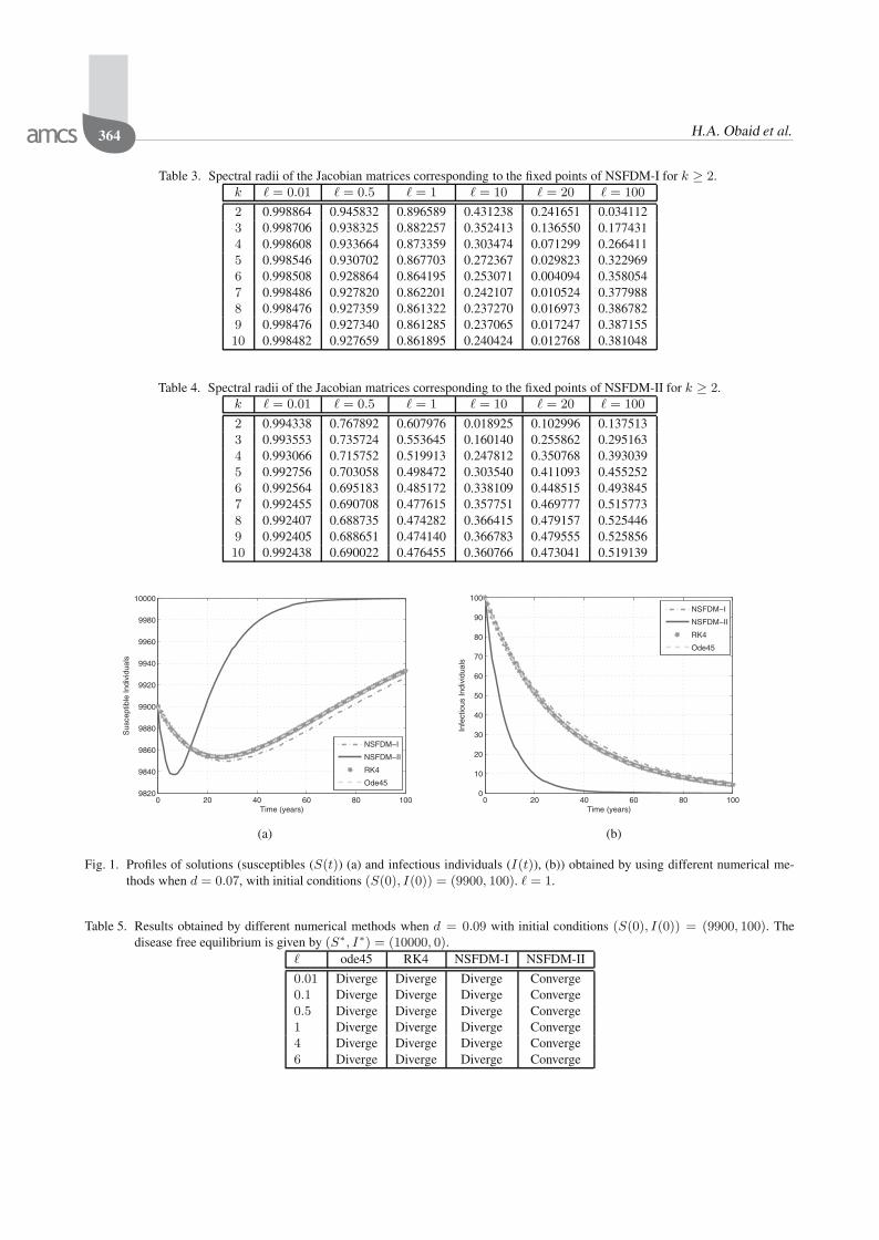
2 1280 1744 −0.1998 −0.08903 1019 1796 −0.2903 −0.08764 866 1827 −0.3652 −0.08815 763 1847 −0.4288 −0.08896 689 1862 −0.4832 −0.08977 633 1873 −0.5296 −0.09048 589 1882 −0.5690 −0.09109 553 1889 −0.6022 −0.091610 523 1895 −0.6298 −0.0922

number of endemic equilibria as presented above in Table2 when R0 > 1. Each of these endemic equilibria islocally asymptotically stable if R0 > 1.

4.2. Numerical stability analysis of the fixed points.The spectral radii of the Jacobian matrices correspondingto the fixed points of the numerical method for differentvalues of Hill coefficient k and the time step-size � aretabulated in this section. We recall from Remark 3 that theequilibria of both systems (1) and (12) remain the samefor any value of k.

It can be seen from the two tables above that all thespectral radii are less than one in magnitude irrespectiveof the time step-size used in the simulations. Hence, eachof these fixed points is locally asymptotically stable ifR0 > 1 for k = 2, 3, . . . , 10. Thus, we have the followingremark.

Remark 6. For k = 2, 3, . . . , 10, each fixed point ofsystem (12) is locally asymptotically stable if R0 >1. Moreover, the system is unconditionally elementarystable.

4.3. Numerical simulations for the disease freeequilibrium. The Disease Free Equilibrium (DFE) iscalculated using the proposed NSFDMs along with othernumerical methods conventionally used. A thoroughcomparison of these methods is presented for manydifferent scenarios. The maximum transmission rate, d,is very important from the biological point of view andhence its value will be varied in a certain range whilekeeping R0 < 1 (as needed for the DFE).

In Section 2, we showed that system (1) has anasymptotically stable disease free equilibrium if R0 < 1.The numerical value of this DFE is given by E∗

0 =(10000, 0). In order to check whether these numericalmethods converge to the theoretical value of the DFE, werequire a tolerance value. To this end, for the susceptiblewe consider their value as 1% of the susceptiblepopulation whereas we consider 20 individuals as thetolerance value for the infectious population. Although

all the numerical methods converge to the disease freeequilibrium, E∗

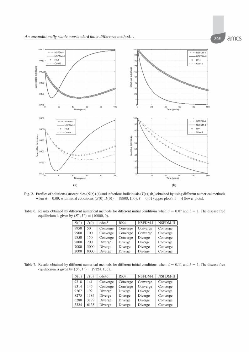
0 , for any time step-size used when d =0.07, we can see from Fig. 1 that only NSFDM-II achievesmuch better convergence. In Table 5 as well as in Fig. 2, itis shown when d = 0.09 only NSFDM-II converges to thecorrect disease free equilibrium, E∗

0 , for different valuesof the step-size.

To see the robustness of the NSFDMs with respect tothe initial conditions, the results are presented in Table 6.In this table we also put the results obtained by the fourthorder Runge–Kutta method and the MATLAB solverode45. It can be seen that NSFDM-II converges for allinitial conditions whereas the others do not. This also canbe seen in Fig. 3.

As far as the positivity of the solutions obtained bythese methods is concerned, we note that the Euler methoddoes not preserve this property although it converges fora wide range of the step-sizes and initial conditions (see,Fig. 4). However, NSFDMs always preserve this property.

4.4. Numerical simulations for the endemic equili-bria. In this section, we study the convergence behaviorof numerical methods to endemic equilibria. We providethe results for various values of the Hill coefficient k.

4.4.1. Case I: Hill coefficient k = 1. When k = 1,the unique endemic equilibrium, E∗, of the system (1) islocally asymptotically stable if d > μ2 (R0 > 1). In thissection, the tolerance values are 1% and 10% for S∗ andI∗, respectively.

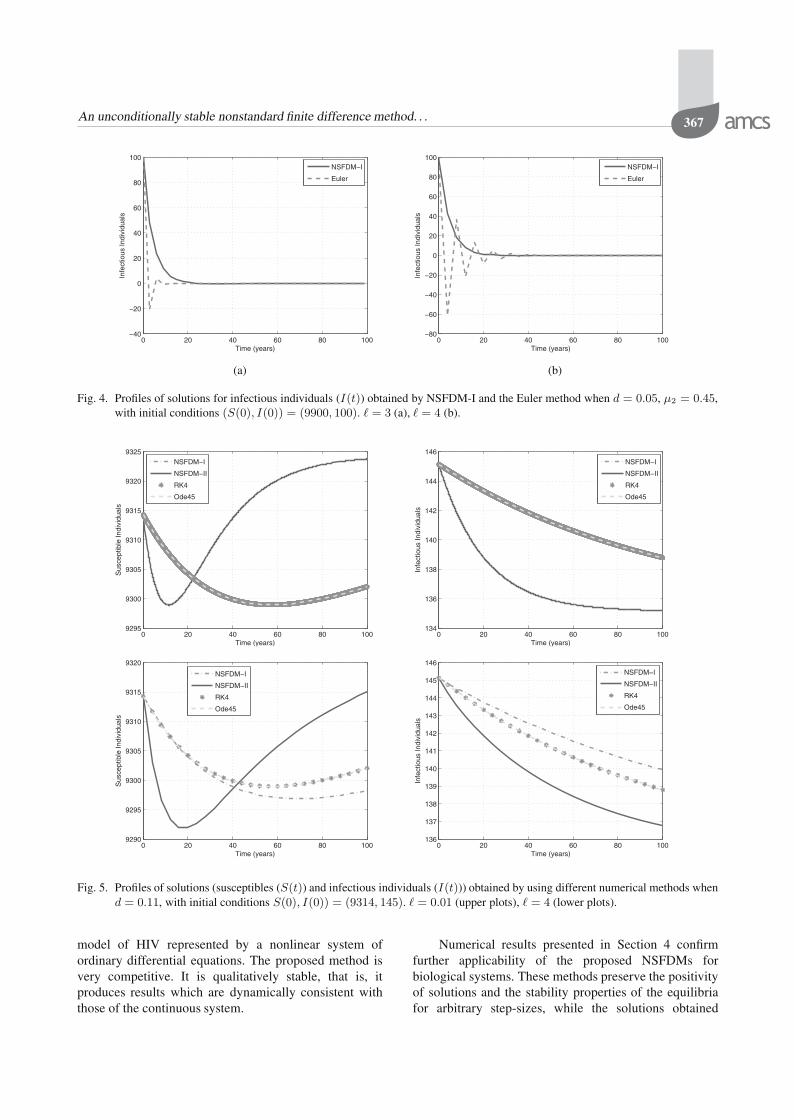
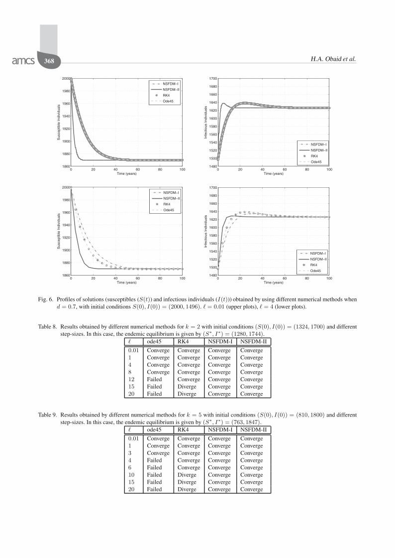
It can be seen from Figs. 5 and 6 that all numericalmethods converge almost to the endemic equilibrium E∗

when d > μ2. However, NSFDM-II converges moreaccurately.

Furthermore, all the numerical methods converge tothe correct endemic equilibrium for any initial conditionsused. However, when d is close to μ2 (which meansthat R0 is close to 1), only NSFDM-II could achieveconvergence for a wide range of the initial conditions.This is shown in Table 7 as well as in Fig. 7. Againas in the case of the DFE, the preservation of thepositivity of the solutions is observed only for NSFDM-I.The Euler method failed to do so although it convergesasymptotically to the correct endemic equilibrium. This isdepicted in Fig. 8 below.

4.4.2. Case II: Hill coefficient k > 1. In this section,simulation results are presented for different numericalmethods for a range of k > 1. As in the previous case, thetolerance value for S∗ is taken as 1%. However, for k > 1,there will be sufficient fluctuations in the dynamics of theinfectious population and therefore we would not take thetolerance as 10% in this case, and hence the 1% tolerancewould suffice for I∗. It can be seen that all the methods in

364 H.A. Obaid et al.

Table 3. Spectral radii of the Jacobian matrices corresponding to the fixed points of NSFDM-I for k ≥ 2.k � = 0.01 � = 0.5 � = 1 � = 10 � = 20 � = 100

2 0.998864 0.945832 0.896589 0.431238 0.241651 0.0341123 0.998706 0.938325 0.882257 0.352413 0.136550 0.1774314 0.998608 0.933664 0.873359 0.303474 0.071299 0.2664115 0.998546 0.930702 0.867703 0.272367 0.029823 0.3229696 0.998508 0.928864 0.864195 0.253071 0.004094 0.3580547 0.998486 0.927820 0.862201 0.242107 0.010524 0.3779888 0.998476 0.927359 0.861322 0.237270 0.016973 0.3867829 0.998476 0.927340 0.861285 0.237065 0.017247 0.38715510 0.998482 0.927659 0.861895 0.240424 0.012768 0.381048

Table 4. Spectral radii of the Jacobian matrices corresponding to the fixed points of NSFDM-II for k ≥ 2.k � = 0.01 � = 0.5 � = 1 � = 10 � = 20 � = 100

2 0.994338 0.767892 0.607976 0.018925 0.102996 0.1375133 0.993553 0.735724 0.553645 0.160140 0.255862 0.2951634 0.993066 0.715752 0.519913 0.247812 0.350768 0.3930395 0.992756 0.703058 0.498472 0.303540 0.411093 0.4552526 0.992564 0.695183 0.485172 0.338109 0.448515 0.4938457 0.992455 0.690708 0.477615 0.357751 0.469777 0.5157738 0.992407 0.688735 0.474282 0.366415 0.479157 0.5254469 0.992405 0.688651 0.474140 0.366783 0.479555 0.52585610 0.992438 0.690022 0.476455 0.360766 0.473041 0.519139

0 20 40 60 80 1009820

9840

9860

9880

9900

9920

9940

9960

9980

10000

Time (years)

Sus

cept

ible

Indi

vidu

als

NSFDM−I

NSFDM−II

RK4

Ode45

0 20 40 60 80 1000

10

20

30

40

50

60

70

80

90

100

Time (years)

Infe

ctio

us In

divi

dual

s

NSFDM−I

NSFDM−II

RK4

Ode45

(a) (b)

Fig. 1. Profiles of solutions (susceptibles (S(t)) (a) and infectious individuals (I(t)), (b)) obtained by using different numerical me-thods when d = 0.07, with initial conditions (S(0), I(0)) = (9900, 100). � = 1.

Table 5. Results obtained by different numerical methods when d = 0.09 with initial conditions (S(0), I(0)) = (9900, 100). Thedisease free equilibrium is given by (S∗, I∗) = (10000, 0).

� ode45 RK4 NSFDM-I NSFDM-II

0.01 Diverge Diverge Diverge Converge0.1 Diverge Diverge Diverge Converge0.5 Diverge Diverge Diverge Converge1 Diverge Diverge Diverge Converge4 Diverge Diverge Diverge Converge6 Diverge Diverge Diverge Converge

An unconditionally stable nonstandard finite difference method. . . 365

0 20 40 60 80 1009750

9800

9850

9900

9950

10000

Time (years)

Sus

cept

ible

Indi

vidu

als

NSFDM−I

NSFDM−II

RK4

Ode45

0 20 40 60 80 1000

10

20

30

40

50

60

70

80

90

100

Time (years)

Infe

ctio

us In

divi

dual

s

NSFDM−I

NSFDM−II

RK4

Ode45

0 20 40 60 80 1009700

9750

9800

9850

9900

9950

Time (years)

Sus

cept

ible

Indi

vidu

als

NSFDM−I

NSFDM−II

RK4

Ode45

0 20 40 60 80 10010

20

30

40

50

60

70

80

90

100

Time (years)

Infe

ctio

us In

divi

dual

s

NSFDM−I

NSFDM−II

RK4

Ode45

(a) (b)

Fig. 2. Profiles of solutions (susceptibles (S(t)) (a) and infectious individuals (I(t)) (b)) obtained by using different numerical methodswhen d = 0.09, with initial conditions (S(0), I(0)) = (9900, 100). � = 0.01 (upper plots), � = 4 (lower plots).

Table 6. Results obtained by different numerical methods for different initial conditions when d = 0.07 and � = 1. The disease freeequilibrium is given by (S∗, I∗) = (10000, 0).

S(0) I(0) ode45 RK4 NSFDM-I NSFDM-II

9950 50 Converge Converge Converge Converge9900 100 Converge Converge Converge Converge9850 150 Converge Converge Diverge Converge9800 200 Diverge Diverge Diverge Converge7000 3000 Diverge Diverge Diverge Converge2000 8000 Diverge Diverge Diverge Converge

Table 7. Results obtained by different numerical methods for different initial conditions when d = 0.11 and � = 1. The disease freeequilibrium is given by (S∗, I∗) = (9324, 135).

S(0) I(0) ode45 RK4 NSFDM-I NSFDM-II

9318 141 Converge Converge Converge Converge9314 145 Converge Converge Converge Converge9267 192 Diverge Diverge Diverge Converge8275 1184 Diverge Diverge Diverge Converge6280 3179 Diverge Diverge Diverge Converge3324 6135 Diverge Diverge Diverge Converge

366 H.A. Obaid et al.

0 10 20 30 40 50 60 70 80 90 1009910

9920

9930

9940

9950

9960

9970

9980

9990

10000

Time (years)

Sus

cept

ible

Indi

vidu

als

NSFDM−I

NSFDM−II

RK4

Ode45

0 10 20 30 40 50 60 70 80 90 1000

5

10

15

20

25

30

35

40

45

50

Time (years)

Infe

ctio

us In

divi

dual

s

NSFDM−I

NSFDM−II

RK4

Ode45

0 10 20 30 40 50 60 70 80 90 1005000

5500

6000

6500

7000

7500

8000

8500

9000

9500

10000

Time (years)

Sus

cept

ible

Indi

vidu

als

NSFDM−I

NSFDM−II

RK4

Ode45

0 10 20 30 40 50 60 70 80 90 1000

500

1000

1500

2000

2500

3000

3500

4000

4500

5000

Time (years)

Infe

ctio

us In

divi

dual

s

NSFDM−I

NSFDM−II

RK4

Ode45

0 20 40 60 80 1002000

3000

4000

5000

6000

7000

8000

9000

10000

Time (years)

Sus

cept

ible

Indi

vidu

als

NSFDM−I

NSFDM−II

RK4

Ode45

0 20 40 60 80 1000

1000

2000

3000

4000

5000

6000

7000

8000

Time (years)

Infe

ctio

us In

divi

dual

s

NSFDM−I

NSFDM−II

RK4

Ode45

(a) (b)

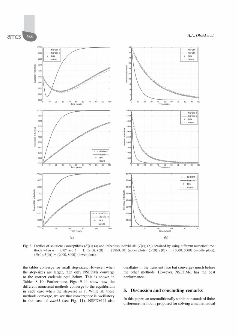
Fig. 3. Profiles of solutions (susceptibles (S(t)) (a) and infectious individuals (I(t)) (b)) obtained by using different numerical me-thods when d = 0.07 and � = 1. (S(0), I(0)) = (9950, 50) (upper plots), (S(0), I(0)) = (5000, 5000) (middle plots),(S(0), I(0)) = (2000, 8000) (lower plots).

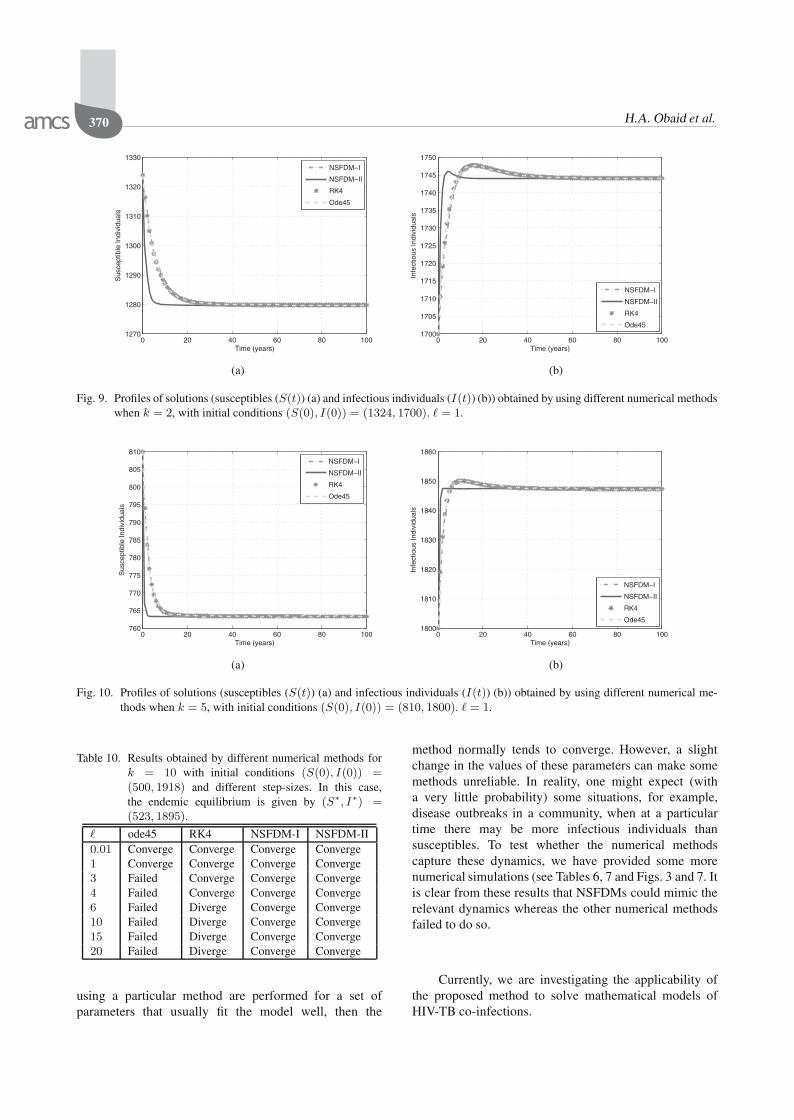
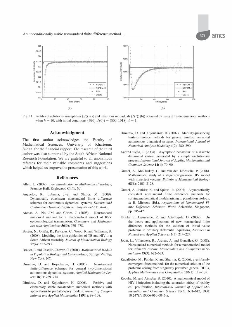
the tables converge for small step-sizes. However, whenthe step-sizes are larger, then only NSFDMs convergeto the correct endemic equilibrium. This is shown inTables 8–10. Furthermore, Figs. 9–11 show how thedifferent numerical methods converge to the equilibriumin each case when the step-size is 1. While all thesemethods converge, we see that convergence is oscillatoryin the case of ode45 (see Fig. 11). NSFDM-II also

oscillates in the transient face but converges much beforethe other methods. However, NSFDM-I has the bestperformance.

5. Discussion and concluding remarks

In this paper, an unconditionally stable nonstandard finitedifference method is proposed for solving a mathematical

An unconditionally stable nonstandard finite difference method. . . 367

0 20 40 60 80 100−40

−20

0

20

40

60

80

100

Time (years)

Infe

ctio

us In

divi

dual

s

NSFDM−I

Euler

0 20 40 60 80 100−80

−60

−40

−20

0

20

40

60

80

100

Time (years)

Infe

ctio

us In

divi

dual

s

NSFDM−I

Euler

(a) (b)

Fig. 4. Profiles of solutions for infectious individuals (I(t)) obtained by NSFDM-I and the Euler method when d = 0.05, μ2 = 0.45,with initial conditions (S(0), I(0)) = (9900, 100). � = 3 (a), � = 4 (b).

0 20 40 60 80 1009295

9300

9305

9310

9315

9320

9325

Time (years)

Sus

cept

ible

Indi

vidu

als

NSFDM−I

NSFDM−II

RK4

Ode45

0 20 40 60 80 100134

136

138

140

142

144

146

Time (years)

Infe

ctio

us In

divi

dual

s

NSFDM−I

NSFDM−II

RK4

Ode45

0 20 40 60 80 1009290

9295

9300

9305

9310

9315

9320

Time (years)

Sus

cept

ible

Indi

vidu

als

NSFDM−I

NSFDM−II

RK4

Ode45

0 20 40 60 80 100136

137

138

139

140

141

142

143

144

145

146

Time (years)

Infe

ctio

us In

divi

dual

s

NSFDM−I

NSFDM−II

RK4

Ode45

Fig. 5. Profiles of solutions (susceptibles (S(t)) and infectious individuals (I(t))) obtained by using different numerical methods whend = 0.11, with initial conditions S(0), I(0)) = (9314, 145). � = 0.01 (upper plots), � = 4 (lower plots).

model of HIV represented by a nonlinear system ofordinary differential equations. The proposed method isvery competitive. It is qualitatively stable, that is, itproduces results which are dynamically consistent withthose of the continuous system.

Numerical results presented in Section 4 confirmfurther applicability of the proposed NSFDMs forbiological systems. These methods preserve the positivityof solutions and the stability properties of the equilibriafor arbitrary step-sizes, while the solutions obtained

368 H.A. Obaid et al.

0 20 40 60 80 1001860

1880

1900

1920

1940

1960

1980

2000

Time (years)

Sus

cept

ible

Indi

vidu

als

NSFDM−I

NSFDM−II

RK4

Ode45

0 20 40 60 80 1001480

1500

1520

1540

1560

1580

1600

1620

1640

1660

1680

1700

Time (years)

Infe

ctio

us In

divi

dual

s

NSFDM−I

NSFDM−II

RK4

Ode45

0 20 40 60 80 1001860

1880

1900

1920

1940

1960

1980

2000

Time (years)

Sus

cept

ible

Indi

vidu

als

NSFDM−I

NSFDM−II

RK4

Ode45

0 20 40 60 80 1001480

1500

1520

1540

1560

1580

1600

1620

1640

1660

1680

1700

Time (years)

Infe

ctio

us In

divi

dual

s

NSFDM−I

NSFDM−II

RK4

Ode45

Fig. 6. Profiles of solutions (susceptibles (S(t)) and infectious individuals (I(t))) obtained by using different numerical methods whend = 0.7, with initial conditions S(0), I(0)) = (2000, 1496). � = 0.01 (upper plots), � = 4 (lower plots).

Table 8. Results obtained by different numerical methods for k = 2 with initial conditions (S(0), I(0)) = (1324, 1700) and differentstep-sizes. In this case, the endemic equilibrium is given by (S∗, I∗) = (1280, 1744).

� ode45 RK4 NSFDM-I NSFDM-II

0.01 Converge Converge Converge Converge1 Converge Converge Converge Converge4 Converge Converge Converge Converge8 Converge Converge Converge Converge12 Failed Converge Converge Converge15 Failed Diverge Converge Converge20 Failed Diverge Converge Converge

Table 9. Results obtained by different numerical methods for k = 5 with initial conditions (S(0), I(0)) = (810, 1800) and differentstep-sizes. In this case, the endemic equilibrium is given by (S∗, I∗) = (763, 1847).

� ode45 RK4 NSFDM-I NSFDM-II

0.01 Converge Converge Converge Converge1 Converge Converge Converge Converge3 Converge Converge Converge Converge4 Failed Converge Converge Converge6 Failed Converge Converge Converge10 Failed Diverge Converge Converge15 Failed Diverge Converge Converge20 Failed Diverge Converge Converge

An unconditionally stable nonstandard finite difference method. . . 369

0 20 40 60 80 1009160

9180

9200

9220

9240

9260

9280

9300

9320

Time (years)

Sus

cept

ible

Indi

vidu

als

NSFDM−I

NSFDM−II

RK4

Ode45

0 20 40 60 80 100130

140

150

160

170

180

190

200

Time (years)

Infe

ctio

us In

divi

dual

s

NSFDM−I

NSFDM−II

RK4

Ode45

0 20 40 60 80 1003000

4000

5000

6000

7000

8000

9000

10000

Time (years)

Sus

cept

ible

Indi

vidu

als

NSFDM−I

NSFDM−II

RK4

Ode45

0 20 40 60 80 1000

1000

2000

3000

4000

5000

6000

7000

Time (years)

Infe

ctio

us In

divi

dual

s

NSFDM−I

NSFDM−II

RK4

Ode45

(a) (b)

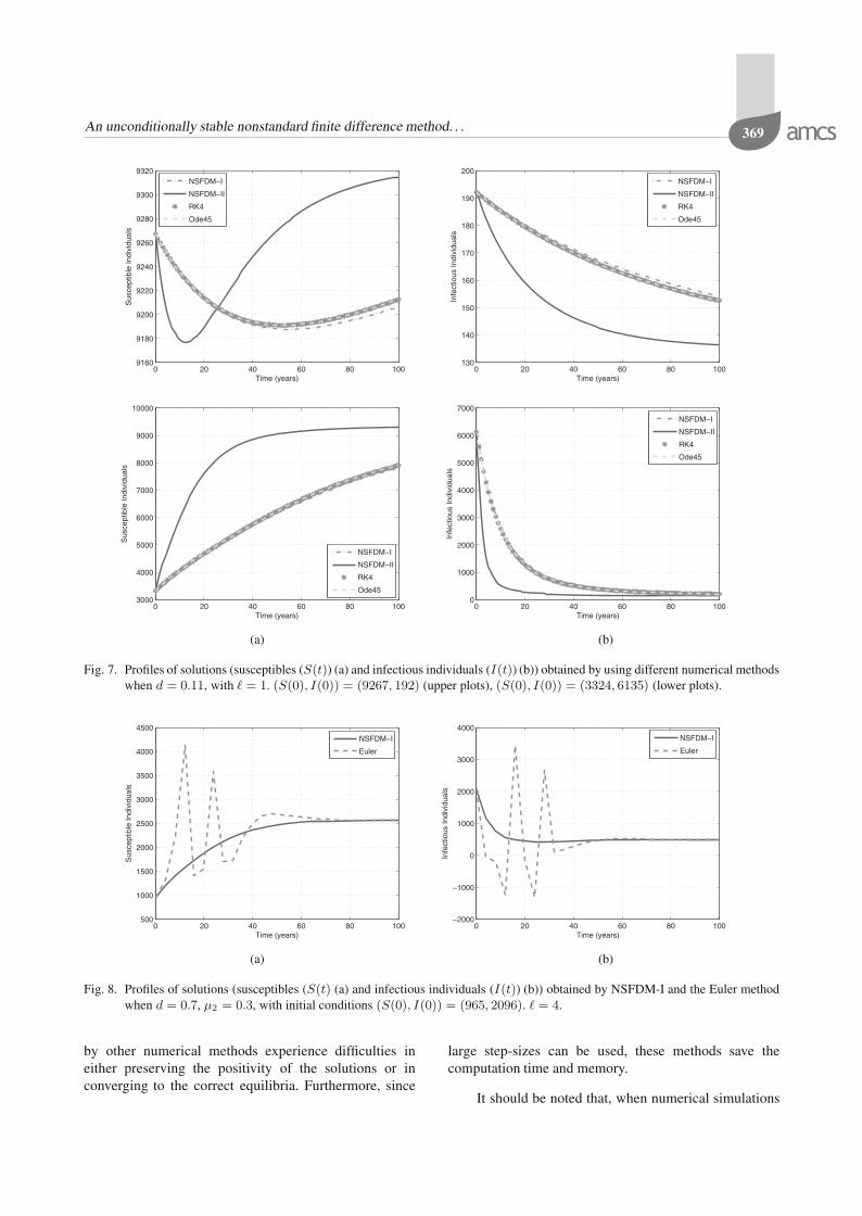
Fig. 7. Profiles of solutions (susceptibles (S(t)) (a) and infectious individuals (I(t)) (b)) obtained by using different numerical methodswhen d = 0.11, with � = 1. (S(0), I(0)) = (9267, 192) (upper plots), (S(0), I(0)) = (3324, 6135) (lower plots).

0 20 40 60 80 100500

1000

1500

2000

2500

3000

3500

4000

4500

Time (years)

Sus

cept

ible

Indi

vidu

als

NSFDM−I

Euler

0 20 40 60 80 100−2000

−1000

0

1000

2000

3000

4000

Time (years)

Infe

ctio

us In

divi

dual

s

NSFDM−I

Euler

(a) (b)

Fig. 8. Profiles of solutions (susceptibles (S(t) (a) and infectious individuals (I(t)) (b)) obtained by NSFDM-I and the Euler methodwhen d = 0.7, μ2 = 0.3, with initial conditions (S(0), I(0)) = (965, 2096). � = 4.

by other numerical methods experience difficulties ineither preserving the positivity of the solutions or inconverging to the correct equilibria. Furthermore, since

large step-sizes can be used, these methods save thecomputation time and memory.

It should be noted that, when numerical simulations

370 H.A. Obaid et al.

0 20 40 60 80 1001270

1280

1290

1300

1310

1320

1330

Time (years)

Sus

cept

ible

Indi

vidu

als

NSFDM−I

NSFDM−II

RK4

Ode45

0 20 40 60 80 1001700

1705

1710

1715

1720

1725

1730

1735

1740

1745

1750

Time (years)

Infe

ctio

us In

divi

dual

s

NSFDM−I

NSFDM−II

RK4

Ode45

(a) (b)

Fig. 9. Profiles of solutions (susceptibles (S(t)) (a) and infectious individuals (I(t)) (b)) obtained by using different numerical methodswhen k = 2, with initial conditions (S(0), I(0)) = (1324, 1700). � = 1.

0 20 40 60 80 100760

765

770

775

780

785

790

795

800

805

810

Time (years)

Sus

cept

ible

Indi

vidu

als

NSFDM−I

NSFDM−II

RK4

Ode45

0 20 40 60 80 1001800

1810

1820

1830

1840

1850

1860

Time (years)

Infe

ctio

us In

divi

dual

s

NSFDM−I

NSFDM−II

RK4

Ode45

(a) (b)

Fig. 10. Profiles of solutions (susceptibles (S(t)) (a) and infectious individuals (I(t)) (b)) obtained by using different numerical me-thods when k = 5, with initial conditions (S(0), I(0)) = (810, 1800). � = 1.

Table 10. Results obtained by different numerical methods fork = 10 with initial conditions (S(0), I(0)) =(500, 1918) and different step-sizes. In this case,the endemic equilibrium is given by (S∗, I∗) =(523, 1895).

� ode45 RK4 NSFDM-I NSFDM-II0.01 Converge Converge Converge Converge1 Converge Converge Converge Converge3 Failed Converge Converge Converge4 Failed Converge Converge Converge6 Failed Diverge Converge Converge10 Failed Diverge Converge Converge15 Failed Diverge Converge Converge20 Failed Diverge Converge Converge

using a particular method are performed for a set ofparameters that usually fit the model well, then the

method normally tends to converge. However, a slightchange in the values of these parameters can make somemethods unreliable. In reality, one might expect (witha very little probability) some situations, for example,disease outbreaks in a community, when at a particulartime there may be more infectious individuals thansusceptibles. To test whether the numerical methodscapture these dynamics, we have provided some morenumerical simulations (see Tables 6, 7 and Figs. 3 and 7. Itis clear from these results that NSFDMs could mimic therelevant dynamics whereas the other numerical methodsfailed to do so.

Currently, we are investigating the applicability ofthe proposed method to solve mathematical models ofHIV-TB co-infections.

An unconditionally stable nonstandard finite difference method. . . 371

0 20 40 60 80 100520

520.5

521

521.5

522

522.5

523

523.5

524

524.5

525

Time (years)

Sus

cept

ible

Indi

vidu

als

NSFDM−I

NSFDM−II

RK4

Ode45

0 20 40 60 80 1001893

1894

1895

1896

1897

Time (years)

Infe

ctio

us In

divi

dual

s

NSFDM−I

NSFDM−II

RK4

Ode45

(a) (b)

Fig. 11. Profiles of solutions (susceptibles (S(t) (a) and infectious individuals (I(t)) (b)) obtained by using different numerical methodswhen k = 10, with initial conditions (S(0), I(0)) = (500, 1918). � = 1.

Acknowledgment

The first author acknowledges the Faculty ofMathematical Sciences, University of Khartoum,Sudan, for the financial support. The research of the thirdauthor was also supported by the South African NationalResearch Foundation. We are grateful to all anonymousreferees for their valuable comments and suggestionswhich helped us improve the presentation of this work.

ReferencesAllen, L. (2007). An Introduction to Mathematical Biology,

Prentice-Hall, Englewood Cliffs, NJ.

Anguelov, R., Lubuma, J.-S. and Shillor, M. (2009).Dynamically consistent nonstandard finite differenceschemes for continuous dynamical systems, Discrete andContinuous Dynamical Systems: Supplement 61: 34–43.

Arenas, A., No, J.M. and Cortés, J. (2008). Nonstandardnumerical method for a mathematical model of RSVepidemiological transmission, Computers and Mathema-tics with Applications 56(3): 670–678.

Bacaer, N., Ouifki, R., Pretorius, C., Wood, R. and Williams, B.(2008). Modeling the joint epidemics of TB and HIV in aSouth African township, Journal of Mathematical Biology57(4): 557–593.

Brauer, F. and Castillo-Chavez, C. (2001). Mathematical Modelsin Population Biology and Epidemiology, Springer-Verlag,New York, NY.

Dimitrov, D. and Kojouharov, H. (2005). Nonstandardfinite-difference schemes for general two-dimensionalautonomous dynamical systems, Applied Mathematics Let-ters 18(7): 769–774.

Dimitrov, D. and Kojouharov, H. (2006). Positive andelementary stable nonstandard numerical methods withapplications to predator–prey models, Journal of Compu-tational and Applied Mathematics 189(1): 98–108.

Dimitrov, D. and Kojouharov, H. (2007). Stability-preservingfinite-difference methods for general multi-dimensionalautonomous dynamical systems, International Journal ofNumerical Analysis Modeling 4(2): 280–290.

Karcz-Duleba, I. (2004). Asymptotic behaviour of a discretedynamical system generated by a simple evolutionaryprocess, International Journal of Applied Mathematics andComputer Science 14(1): 79–90.

Gumel, A., McCluskey, C. and van den Driessche, P. (2006).Mathematical study of a staged-progression HIV modelwith imperfect vaccine, Bulletin of Mathematical Biology68(8): 2105–2128.

Gumel, A., Patidar, K. and Spiteri, R. (2005). Asymptoticallyconsistent nonstandard finite difference methods forsolving mathematical models arising in population biology,in R. Mickens (Ed.), Applications of Nonstandard Fi-nite Difference Schemes, World Scientific, Singapore,pp. 385–421.

Ibijola, E., Ogunrinde, R. and Ade-Ibijola, O. (2008). Onthe theory and applications of new nonstandard finitedifference methods for the solution of initial valueproblems in ordinary differential equations, Advances inNatural and Applied Sciences 2(3): 214–224.

Jódar, L., Villanueva, R., Arenas, A. and González, G. (2008).Nonstandard numerical methods for a mathematical modelfor influenza disease, Mathematics and Computers in Si-mulation 79(3): 622–633.

Kadalbajoo, M., Patidar, K. and Sharma, K. (2006). ε-uniformlyconvergent fitted methods for the numerical solution of theproblems arising from singularly perturbed general DDEs,Applied Mathematics and Computation 182(1): 119–139.

Kouche, M. and Ainseba, B. (2010). A mathematical model ofHIV-1 infection including the saturation effect of healthycell proliferation, International Journal of Applied Ma-thematics and Computer Science 20(3): 601–612, DOI:10.2478/v10006-010-0045-z.

372 H.A. Obaid et al.

Lubuma, J.-S. and Patidar, K. (2006). Uniformly convergentnon-standard finite difference methods for self-adjointsingular perturbation problems, Journal of Computationaland Applied Mathematics 191(2): 229–238.

Lubuma, J.-S. and Patidar, K. (2007a). Non-standardmethods for singularly perturbed problems possessingoscillatory/layer solutions, Applied Mathematics and Com-putation 187(2): 1147–1160.

Lubuma, J.-S. and Patidar, K. (2007b). Solving singularlyperturbed advection reaction equation via non-standardfinite difference methods, Mathematical Methods in theApplied Sciences 30(14): 1627–1637.

Lubuma, J.-S. and Patidar, K. (2007c). ε-uniform non-standardfinite difference methods for singularly perturbednonlinear boundary value problems, Advances in Mathe-matical Sciences and Applications 17(2): 651–665.

Mickens, R. (2007). Calculation of denominator functionsfor nonstandard finite difference schemes for differentialequations satisfying a positivity condition, Numerical Me-thods for Partial Differential Equations 23(3): 672–691.

Mickens, R. and Ramadhani, I. (1994). Finite-differenceschemes having the correct linear stability properties forall finite step-sizes III, Computer in Mathematics with Ap-plications 27(4): 77–84.

Mickens, R. and Smith, A. (1990). Finite differencemodels of ordinary differential equations: Influence ofdenominator functions, Journal of the Franklin Institute327(1): 143–145.

Munyakazi, J. and Patidar, K. (2010). Higher order numericalmethods for singularly perturbed elliptic problems, Neural,Parallel & Scientific Computations 18(1): 75–88.

Patidar, K. (2005). On the use of nonstandard finite differencemethods, Journal of Difference Equations and Applica-tions 11(8): 735–758.

Patidar, K. (2008). A robust fitted operator finite differencemethod for a two-parameter singular perturbationproblem, Journal of Difference Equations and Applica-tions 14(12): 1197–1214.

Patidar, K. and Sharma, K. (2006a). Uniformly convergentnonstandard finite difference methods for singularlyperturbed differential difference equations with delay andadvance, International Journal for Numerical Methods inEngineering 66(2): 272–296.

Patidar, K. and Sharma, K. (2006b). ε-uniformly convergentnon-standard finite difference methods for singularlyperturbed differential difference equations withsmall delay, Applied Mathematics and Computation175(1): 864–890.

Rauh, A., Brill, M. and Günther, C. (2009). A novel intervalarithmetic approach for solving differential-algebraicequations with ValEncIA-IVP, International Journal of Ap-plied Mathematics and Computer Science 19(3): 381–397,DOI: 10.2478/v10006-009-0032-4.

Rauh, A., Minisini, J. and Hofer, E.P. (2009). Verificationtechniques for sensitivity analysis and design of

controllers for nonlinear dynamic systems withuncertainties, International Journal of Applied Ma-thematics and Computer Science 19(3): 425–439, DOI:10.2478/v10006-009-0035-1.

Villanueva, R., Arenas, A. and Gonzalez-Parra, G. (2008).A nonstandard dynamically consistent numerical schemeapplied to obesity dynamics, Journal of Applied Mathema-tics, Article ID 640154, DOI: 10.1155/2008/640154.

Xu, C., Liao, M. and He, X. (2011). Stability and Hopfbifurcation analysis for a Lotka–Volterra predator-preymodel with two delays, International Journal of AppliedMathematics and Computer Science 21(1): 97–107, DOI:10.2478/v10006-011-0007-0.

Zhai, G. and Michel, A.M. (2004). Generalized practicalstability analysis of discontinuous dynamical systems, In-ternational Journal of Applied Mathematics and ComputerScience 14(1): 5–12.

Hasim Obaid obtained his M.Sc. in industrial and computational ma-thematics in 2003 from the University of Khartoum, Sudan, and hisPh.D. in 2011 from the University of the Western Cape, South Afri-ca. His research interests include mathematical analysis of models ari-sing in biology specially those describing HIV and tuberculosis diseases,and developing some numerical methods to approximate the solutions ofsuch biological models.

Rachid Ouifki is a senior researcher at theDST/NRF Centre of Excellence in Epidemiologi-cal Modelling and Analysis (SACEMA) at Stel-lenbosch University, South Africa. He holds aPh.D. degree in applied mathematics. He is a co-author of several papers and a regular reviewerfor some scientific journals. He is also involvedin several international projects. His current re-search includes ordinary, delayed and partial dif-ferential equations and their applications with a

particular focus to bio-mathematics. He also works on optimal controltheory and its applications, especially in the control of infectious dise-ases.

Kailash Patidar is a professor of applied mathe-matics at the University of the Western Cape, So-uth Africa. His research is focused on numericalmethods and scientific computing for the appliedproblems that arise from interactions between na-tural and life sciences as well as engineering. Hisresearch is a well balanced combination of ana-lytical investigations and numerical experimentsusing finite difference, finite element and splineapproximation methods. His current research in-

volves the development of reliable numerical methods for mathematicalmodels arising in population biology as well as those for option pricingproblems in computational finance.

Received: 21 March 2012Revised: 17 December 2012