8/20/2019 AN5141 Spec

http://slidepdf.com/reader/full/an5141-spec 1/12

Maxim > Design Support > Technical Documents > Application Notes > Automatic Test Equipment (ATE) > APP 5141

Keywords: SPICE, simulation, cable model, skin effect, lumped model, transmission line, dielectric loss 

 APPLICATION NOTE 5141

 An Improved and Simple Cable Simulation ModelBy: Bernard Hyland, Senior Member of Technical Staff 

Oct 22, 2012

 Abstract: Nonideal cable dispersive effects can affect system performance. This application note discusses the two

main loss effects related to cables (skin-effect and dielectric losses), and presents a simple method of modeling the

cable for use in standard SPICE simulators. 

 A similar version of this article appears on EDN, July 30, 2012.

Introduction

Cables are used in many high-frequency board designs and can become a critical element in the signal path. This is

especially true for signals that exceed 500MHz. If not modeled as part of that system, cables can lead to unexpected

system performance degradation and to costly time delays in debugging and corrections. Even with this understood,

cables are notoriously difficult to model correctly. Using a simple transmission line model may not effectively model this

element because it is difficult to model a cable both in the frequency and the time domains.

Cable nonideal dispersive effects can affect system performance. These cable effects are seen¹ on drivers, buffers, and

comparators. In the driver or buffer, the low-frequency dribble up (Figure 1) primarily degrades propagation delay

versus pulse-width dispersion; it also degrades minimum pulse time and rise time. In the comparator, the low-

frequency dribble up primarily degrades delay versus pulse width and propagation delay versus overdrive; it also

degrades the minimum pulse width. This application note will discuss the two main loss effects related to cables: the

skin effect and dielectric losses. We will then present a simple method of modeling the cable for use in standard

SPICE simulators.

Figure 1. Example of cable loss effects (simulated results from Figure 3 below).

Why Model a Cable?

 As frequencies start to exceed 500MHz, the cable starts to noticeably impact the bandwidth of the signal path and

begins to degrade this path in many ways. To understand the effects of cables at all frequencies, the cable needs to

be modeled. However, based on that model, more intelligent decisions can be made about the type of cable to be

used. Moreover, the parameters of interest that are being degraded in the signal path can then be understood.

Page 1 of 12

8/20/2019 AN5141 Spec

http://slidepdf.com/reader/full/an5141-spec 2/12

Cable Losses

There are two main loss mechanisms with cables: skin-effect and dielectric losses.

Skin-Effect Losses

 At high frequencies, the signal tends to propagate along the surface of the conductor. This is known as skin effect.

(Note that this application note will not rigorously discuss skin-effect losses.) The skin depth, δ, is defined as:

(Eq. 1)

Where ω is the frequency in radian per second; µ is the conductor's permeability in H (Henries per meter); and σ isthe conductor's conductivity in S (Siemens per meter).

Equation 1 shows that the skin depth decreases with the square root of the frequency. Alternatively, since the lower 

the skin depth the higher the resistance per unit length, then the resistance per unit length, RL, increases with the

square root of frequency.

Therefore, RL = 1/Wδσ, where W is the conductor's cross-sectional width (for a circular wire, W = 2 πr). Rewriting:

(Eq. 2)

Dielectric Loss

The dielectric constant of insulators has an imaginary component. The dielectric constant, ε, is defined as ε = ε' + jε'' =ε'(1 + jtanδ), where ε' is the real component of the dielectric constant; and tand is the loss tangent or dissipation factor of the dielectric. The dielectric constant affects the capacitance and the Cl (capacitance per unit length) will change to

Cl(1 + jtanδ).

Total Cable LossBy including the skin-effect and dielectric losses in the model, an ideal cable model (per unit length) can be now

modified to include those losses (Figure 2). Here L l, R l, and Cl are the per unit length for inductance, resistance, and

capacitance, respectively.

Figure 2. Ideal cable representation.

The propagation constant is defined as jk = √ZY, where Z is the distributed series impedance and Y is the distributedparallel admittance.

From Figure 2 we see:

(Eq. 3)

Using a Taylor-Expansion approximation:

Page 2 of 12

8/20/2019 AN5141 Spec

http://slidepdf.com/reader/full/an5141-spec 3/12

(Eq. 4)

Further simplifying:

(Eq. 5)

Where Zo is the cable's characteristic impedance; εr  is the relative dielectric constant; and c is the speed of light.

We are actually seeking the cable gain, H(ƒ). Therefore, H(ƒ) = e-jkl, where l is the length of the line.

Using the findings above:

(Eq. 6)

Where:

(Eq. 7 and 8)

Therefore, skin-effect losses (α1) dominate at lower frequencies and dielectric losses (α2) dominate at higher 

frequencies.

Note that in real-world cables H(ƒ) varies somewhat from the approximations given above. However, this model is

accurate enough for most automated-test-equipment (ATE) work, where the attenuation increases to 6dB at the most.

We will be using Equations 6, 7, and 8 later to model the cable.

SPICE Approximations

Unfortunately, H(ƒ) cannot be modeled well in the time-domain SPICE and electromagnetic (EM) simulators. Typical

EM simulators generate a lumped transmission line approximation. The lumps must be small enough to look like a

transmission line at the frequency of interest, and the lumped elements must vary with frequency. This typically

generates a very big model for longer lines.

S-parameter data from manufacturers can also be used to model the frequency response of the cable. But S-

parameters only model the AC response and not the transient response. S-parameter extraction requires very accurate

equipment, setups, and calibrations, and is not always readily available. You also need to have a different set of S-

parameters for each cable length, which again is difficult to obtain.

 Alternatively, H(ƒ) can be approximated by a multiple-pole/zero-fit network. This pole/zero network models both the AC

and transient performance. The pole/zero fits the magnitude very well, but the phase-fit error can be significant.

Because the phase is linear with frequency, it appears as an ideal transmission line and can, thus, be eliminated. A -

3dB pole/zero fit matched an EM simulator within 3 degrees phase error up to the -3dB point.

There are two notable shortcomings to a pole/zero network model:

1. The pole/zero network does not include the ideal phase-dependent part of H(ƒ)—the part that varies linearly with

frequency. This is usually not needed, since the ideal phase lag looks like an ideal transmission line. If the phase

of H(ƒ) is needed, add an ideal transmission line in series with the pole/zero network.

2. The pole/zero network assumes matched characteristic impedance over all frequencies. L l changes with

frequency. For reasonable losses (less than 6dB), the change in L l is insignificant. For larger losses, the pole/zero

network would err.

Page 3 of 12

8/20/2019 AN5141 Spec

http://slidepdf.com/reader/full/an5141-spec 4/12

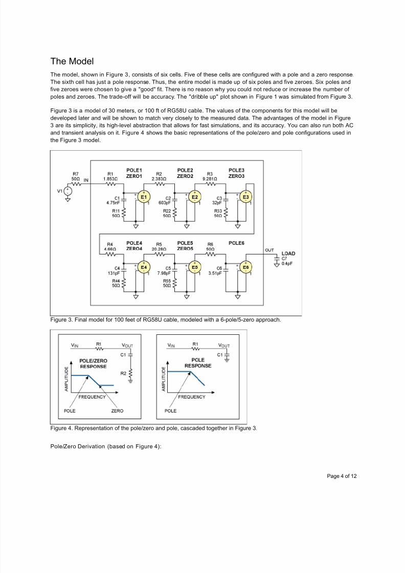
The Model

The model, shown in Figure 3, consists of six cells. Five of these cells are configured with a pole and a zero response.

The sixth cell has just a pole response. Thus, the entire model is made up of six poles and five zeroes. Six poles and

five zeroes were chosen to give a "good" fit. There is no reason why you could not reduce or increase the number of 

poles and zeroes. The trade-off will be accuracy. The "dribble up" plot shown in Figure 1 was simulated from Figure 3.

Figure 3 is a model of 30 meters, or 100 ft of RG58U cable. The values of the components for this model will be

developed later and will be shown to match very closely to the measured data. The advantages of the model in Figure

3 are its simplicity, its high-level abstraction that allows for fast simulations, and its accuracy. You can also run both AC

and transient analysis on it. Figure 4 shows the basic representations of the pole/zero and pole configurations used in

the Figure 3 model.

Figure 3. Final model for 100 feet of RG58U cable, modeled with a 6-pole/5-zero approach.

Figure 4. Representation of the pole/zero and pole, cascaded together in Figure 3.

Pole/Zero Derivation (based on Figure 4):

Page 4 of 12

8/20/2019 AN5141 Spec

http://slidepdf.com/reader/full/an5141-spec 5/12

VOUT/VIN = (1 + R2 × C1 × S)/(1 + (R1 + R2) × C1 × S)

Pole = 1/(2 × π × (R1 + R2) × C1), Zero = 1/(2 × π × R2 × C1)

Pole Derivation (based on Figure 4)

VOUT/VIN = 1/(1 + R1 × C1 × S)

Pole = 1/(2 × π × R1 × C1)

Figure 5 shows the conceptual and graphical representation of how the pole/zero concept is fitted to the real response.

Note that we are modeling a 30m or 100ft. RG58U cable. As will be seen by the GNUPLOT-generated plot, the fit is

very good all the way out to better than -30dB. In general, it is more accurate to model cables out to -6dB.

Figure 5. Graphical representation shows how the 6-pole/5-zero model fits the real response.

Derivation of the Model

 Appendix A  is a GNUPLOT file that uses the physical constants of the cable. In this example, we use the RG58U

cable and mathematically define the cable response utilizing Equations 6, 7, and 8 above. It then plots this response.

The GNUPLOT file mathematically models the pole/zero and pole responses, as shown in Figure 3, and then calculates

the values of the Rs and Cs. The calculation involves the use of the GNUPLOT "FIT" function. This function will do a

least-square fit to find the poles and the zeroes. It will plot this calculated response, or "fit," and overlay this on the

cable's response, as defined by the physical parameters. Appendix A shows that the real response of the cable,

defined by the cable's physical properties, is accurately matched by the least-square fit, based on a 6 pole/5 zero fit.

Finally the GNUPLOT file calculates the R and C values for Figure 3, which then becomes the model and can be

simulated by any SPICE simulator. Finally, we overlay the real cable response, the least-square approximation, and

then the simulated plot from the model. It will be shown that all three plots agree very closely and, hence, confirm the

model.

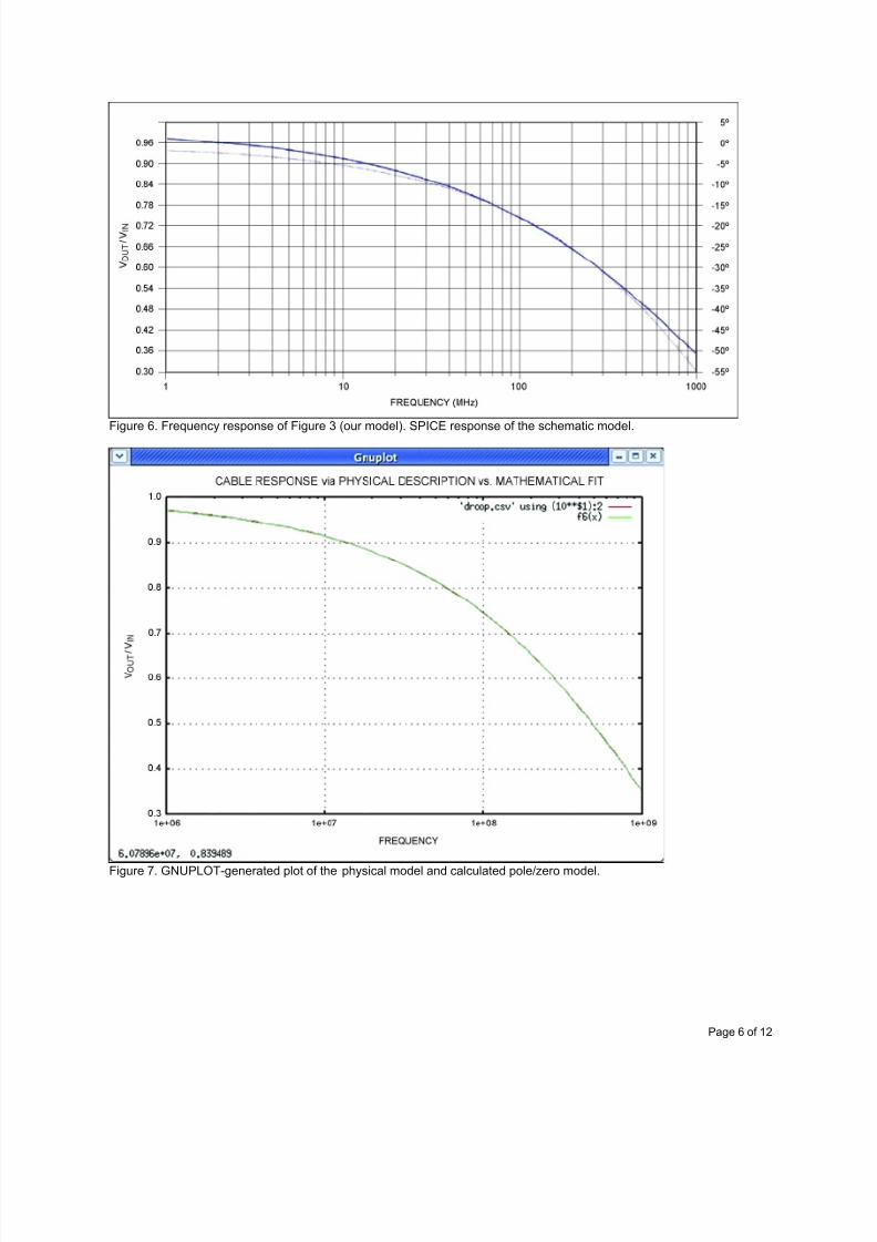
Figures 6 and 7 are SPICE simulations from the derived model of the 100ft. RG58U cable.

Page 5 of 12

8/20/2019 AN5141 Spec

http://slidepdf.com/reader/full/an5141-spec 6/12

Figure 6. Frequency response of Figure 3 (our model). SPICE response of the schematic model.

Figure 7. GNUPLOT-generated plot of the physical model and calculated pole/zero model.

Page 6 of 12

8/20/2019 AN5141 Spec

http://slidepdf.com/reader/full/an5141-spec 7/12

Figure 8. AC input impedance plot of Figure 3 (our model); SPICE response of the schematic model.

Procedure to Create the Model

1. Obtain manufacturer's data for the physical characteristics of the cable:

Magnetic permeability (u = 1.2e6H/m)

Speed of light (c = 300me6 mps)

Conductivity of the signal wire (copper = sigma = 58.6e6 spm)

Characteristic impedance of the cable (for RG58U = 50Ω)

Relative dielectric constant for the insulator material (for RG58U, er = 2.3 for solid polyethylene)

Loss tangent of the insulator (for RG58U, tand = 0.00035)

Signal cable width (for RG58U = 4.5e × 10 -4  m = 0.00045m)

Cable length: this will be the only parameter that will vary and can be passed.

2. Run the GNUPLOT program in Appendix A.

Create the first estimates for wp1 to wp6 and wz1 to wz5 (poles and zeroes). The program in Appendix A

already has these first estimates.

If the error as shown in Append ix B  is greater than a few percent, insert the calculated poles and zeros

back into the GNUPLOT program and run and reiterate until the error is below a few %. If you do not do this

and have large errors in the calculated "fit," you will get errors in the calculations of the Rs and Cs for the

final model.

 Adjust the Rs and Cs as calculated in the GNUPLOT program in Appendix A and printed in Appendix B into

the Figure 3 schematic.

Run an AC sim for Figure 3. Review that the frequency response matches the GNUPLOT responses, as

shown in Figures 6 and 7. If they agree, you are done.

3. You can then run various lengths of the cable to create new models for these different lengths. The schematic

becomes the model and will show both transient and frequency characteristics of the cable.

Summary

This application note showed a simple approach to modeling a signal cable by obtaining just the physical data for that

cable. This process extends to all cables. A cable signal's characteristics are defined by its physical construction and

the materials used. The more normal approach is to obtain S-parameter sweeps or create distributed RLC elements to

model the cable. These do have their place. S-parameters are limited to AC analysis only and must be redone for 

Page 7 of 12

8/20/2019 AN5141 Spec

http://slidepdf.com/reader/full/an5141-spec 8/12

every cable and length of that cable. The major limitation of S-parameters is their lack of transient information. S-

parameters can be hard to retrieve. Either the manufacturer supplies these parameters or you must have expensive

equipment to extract these parameters and perform methodical calibration routines. Distributed models allow for AC and

transient modeling, but they are difficult to obtain. Distributed models to obtain an accurate model can also be quite

large and slow down SPICE simulations tremendously.

The greatest advantage of the model presented here is that none of the above restrictions apply. Rather, you get or 

determine:

1. A simple modeling interface

2. Need only obtain the physical information of the cable.

3. The pole/zero fit provides a very accurate model of the loss response.

4. The model parameters for the poles and zeros are easily calculated to create the schematic.

5. The only parameter in this model is the length of the cable.

6. It is easy to compose a library of cables from the physical parameters and pass these calculated Rs and Cs to a

circuit that remains the same.

7. Quick, easy "what if analysis" right at your bench

8. Can easily be ported to MATLAB® for greater GUI flexibility.

This model does have its limitations, as discussed. Many versions of cable models can be more accurate, but they also

can be very complex and unwieldy. This approach gives a very simple method for modeling a cable, and the methodhas very good accuracy over at least a -6dB loss. While it models well past this loss, you would have to account for 

impedance and phase differences if these impact the design.

Reference

¹These cable effects have been seen often by the ATE group at Maxim Integrated. This application note, in fact,

represents its findings; the cable model was developed and tested extensively by that group.

The author would like to acknowledge Charles Sharman, former employee of Maxim Integrated, for his original concept

of a multipole, multizero filter to model the coaxial cable.

 Appendix A. GNUPLOT File# GNUPLOT Fi l e t hat :

#1) Cal cul at es t he f r equency response af t er cal cul at i ng t he ski n ef f ect and di el ect r i c

ef f ects,

usi ng onl y t he physi cal parameter s of t he cabl e.

#2) I t t hen pl ots t he f r equency r esponse caused by t hese physi cal parameters and st ores

t hat

i nf or mat i on i n a f i l e cal l ed dr oop. csv.

#3) We t hen def i ne a pol e/ zero and pol e r esponse, based on f r equency, t he pol e, and t he

zero.

#4) We cascade f i ve pol e/ zer oes and one pol e.

#5) We t hen cal cul ate t he si x pol es ( wp1 t o wp6) and the f i ve zer oes ( wz1 t o wz2) usi ng

t he

GNUPLOT "Fi t " f unct i on.#6) We t hen cal cul ate a SPI CE- equi val ent schemat i c wi t h Rs and Cs def i ned by t he pol es

and zer oes.

#7) We pl ot t he cal cul ated physi cal r esponse and over l ay t hat wi t h the mathemat i cal l y

cal cul at ed

f i t , based on a 6 pol e/ 5 pol e f i t .

#8) The Rs and Cs are passed ont o a SPI CE hi gh- l evel schemat i c, and t hi s model s t he

cabl e. Thi s

Page 8 of 12

8/20/2019 AN5141 Spec

http://slidepdf.com/reader/full/an5141-spec 9/12

schemat i c can t hen r un AC or t r ansi ent si mul at i ons.

#9) Last l y, we run t he SPI CE model and obtai n the r esponse and compar e t hi s t o t he

physi cal

r esponse and the mathemat i cal r esponse. Al l t hr ee responses must l i e on t op of one

another t o

ensure a good model f i t .

# Frequenci es of i nt erestf mi n = 1e+6 # mi ni mum f r equency ( Hz)

f max = 1e9 # maxi mum f r equency ( Hz)

# Physi cal const ant s

u=1. 26e- 6 # magnet i c permeabi l i t y ( H/ m)

c=300e+6 # speed of l i ght ( m/ s)

# Li ne- speci f i c const ant s f or cabl e

si gma=58e+6 # copper conduct i vi t y ( S/ m)

z0=50 # charact er i st i c i mpedance ( Ohms)

er=2. 3 # r el ati ve di el ect r i c const ant RG58U cabl e ( sol i d Pol yet hyl ene)

t and=0. 00035 # l oss t angent / di ssi pati on f act or ( pol yet hyl ene)

w=2*pi *4. 5*10- 4 # cr oss- sect i onal cabl e wi dt h (m)#l i s l i ne l engt h ( m)

l =30

# At t enuat i on const ant s

a1=( l / ( 2*w*z0) ) *sqr t ( pi *u/ si gma) # ski n ef f ect . Same as Equat i on 6.  

a2=(l *pi *tand*sqrt ( er) ) / c # Di el ectr i c Ef f ect. Same as Equat i on 7.

pr i nt "a1=", a1

pr i nt "a2=", a2

# Pl ot t he l oss i ncl udi ng ski n and di el ectr i c eff ects

pl ot [ f =f mi n: f max] exp( - a1*sqr t ( f ) - a2*f ) # Pl ot t i ng Equat i on 8.

set t er mi nal t abl e

set l ogscal e x

set out put ' dr oop. csv'

set t i t l e " Cabl e Response vi a Physi cal Descri pt on vs Mat hemat i cal Fi t "

set xl abel "Fr equency"; set yl abel "Ampl i t ude ( v)"

set xrange [ 1e6: 1e9]

#Setup f or pl ott i ng t o t ermi nal

repl ot

set t ermi nal x11

set out put

f scal e=1e9

# Def i ne pol e zer o and pol e equat i ons

# pol e/ zero

pz(x, p, z)=( 1+( ( 2*pi *x) / ( 2*pi *z)) **2) / ( 1+( ( 2*pi *x) / ( 2*pi *p) ) **2)

# pol e

p( x, p) =1/ ( 1+( ( 2*pi *x)/ ( 2*pi *p) ) **2) # Eq2

Page 9 of 12

8/20/2019 AN5141 Spec

http://slidepdf.com/reader/full/an5141-spec 10/12

# 6- pol e f i t - cascadi ng 6 pol e/ zer o and one pol e ut i l i zi ng pz( x. p. z) and p( x, p) . Wher e

x i s t he f r equency.

f 6( x)=sqrt ( pz( x, wp1, wz1)* pz( x, wp2, wz2)*pz( x, wp3, wz3)* pz( x, wp4, wz4)* pz( x, wp5, wz5)* p( x, wp6) )

# Def i ne our i ni t i al est i mat es

wp1=7e- 3*f scal e; wz1=8e- 3*f scal e; wp2=6e- 2*f scal e; wz2=7e- 2*f scal e; wp3=2. 5e- 1*f scal e;

wz3=3. 5e- 1*f scal e;

wp4=. 25*f scal e; wz4=0. 1*f scal e; wp5=. 5*f scal e; wz5=1*f scal e; wp6=12*f scal e# Cal l GNUPLOT' s "f i t " f unct i on t o cal cul ate pol es and zer oes by l east square method

f i t f 6( x) ' dr oop. csv' usi ng ( 10**$1) : 2 vi a wp1, wz1, wp2, wz2, wp3, wz3, wp4, wz4, wp5,

wz5, wp6

#Over l ay the Cabl e Characteri st i cs vs t he Mathemati cal Fi t .

pl ot ' dr oop. csv' usi ng (10**$1) : 2, f 6( x)

#Cal cul ate Rs and Cs f or pol e/ zero schemat i c nor mal i zed f or a 50 ohm characteri st i c

i mpedance.

#Pol e Zer o1

r 1= 50*( ( wz1/ wp1) - 1) ; c1=1/ ( 2*pi *50*wz1)

#Pol e Zer o2r 2= 50*( ( wz2/ wp2) - 1) ; c2=1/ ( 2*pi *50*wz2)

#Pol e Zer o3

r 3= 50*( ( wz3/ wp3) - 1) ; c3=1/ ( 2*pi *50*wz3)

#Pol e Zer o4

r 4= 50*( ( wz4/ wp4) - 1) ; c4=1/ ( 2*pi *50*wz4)

#Pol e Zer o1

r 5= 50*( ( wz5/ wp5) - 1) ; c5=1/ ( 2*pi *50*wz5)

#Last Pol e

c6=1/ ( 2*pi *50*wp6)

pr i nt "r 1=", r 1; pr i nt "c1=", c1

pr i nt "r 2=", r 2; pr i nt "c2=", c2pr i nt "r 3=", r 3; pr i nt "c3=", c3

pr i nt "r 4=", r 4; pr i nt "c4=", c4

pr i nt "r 5=", r 5; pr i nt "c5=", c5

pr i nt "c6=", c6

pause - 1 ' Hi t r et ur n t o cont i nue'

 Appendix B. Output Log of GNUPLOT File Run in Appendix AAf t er 480 i t er at i ons t he fi t conver ged.

Fi nal sum of squar es of r esi dual s: 5. 84016e- 06

Rel . change dur i ng l ast i t er at i on: - 4. 6111e- 06

Degr ees of f r eedom ( ndf ) : 89

r ms of r esi dual s ( st df i t ) = sqr t ( WSSR/ ndf ) : 0. 000256164

Vari ance of r esi dual s ( r educed chi square) = WSSR/ ndf : 6. 56198e- 08

Page 10 of 12

8/20/2019 AN5141 Spec

http://slidepdf.com/reader/full/an5141-spec 11/12

8/20/2019 AN5141 Spec

http://slidepdf.com/reader/full/an5141-spec 12/12

MAX9268 Gigabit Multimedia Serial Link Deserializer with LVDS System

Interface

 

MAX9979 Dual 1.1Gbps Pin Electronics with Integrated PMU and Level-

Setting DACs

Free Samples 

More Information

For Technical Support: http://www.maximintegrated.com/support

For Samples: http://www.maximintegrated.com/samples

Other Questions and Comments: http://www.maximintegrated.com/contact 

 Application Note 5141: http://www.maximintegrated.com/an5141

 APPLICATION NOTE 5141, AN5141, AN 5141, APP5141, Appnote5141, Appnote 5141 

Copyright © by Maxim Integrated

 Additional Legal Notices: http://www.maximintegrated.com/legal

Page 12 of 12