Embed Size (px)
Citation preview

Analysis of community ecology data in R
Jinliang Liu (刘金亮)
Institute of Ecology, College of Life ScienceZhejiang University
Email: [email protected]://jinliang.weebly.com
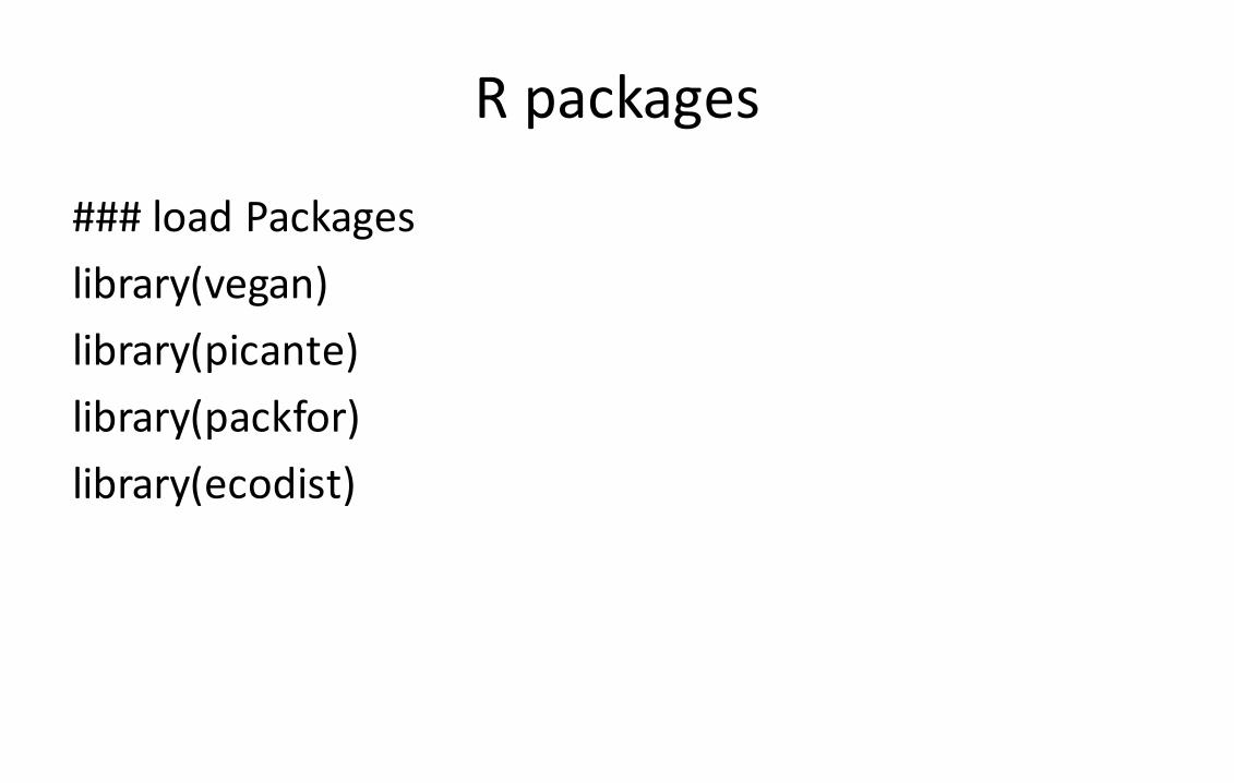
Rpackages
###loadPackageslibrary(vegan)library(picante)library(packfor)library(ecodist)
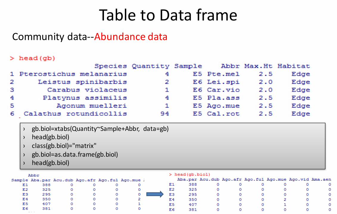
TabletoDataframe
› gb.biol=xtabs(Quantity~Sample+Abbr, data=gb)› head(gb.biol)› class(gb.biol)="matrix"› gb.biol=as.data.frame(gb.biol)› head(gb.biol)
Communitydata--Abundancedata
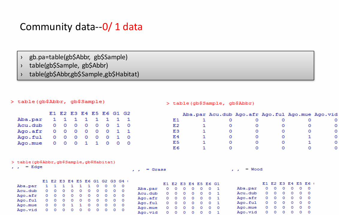
Communitydata--0/1data
› gb.pa=table(gb$Abbr, gb$Sample)› table(gb$Sample, gb$Abbr)› table(gb$Abbr,gb$Sample,gb$Habitat)
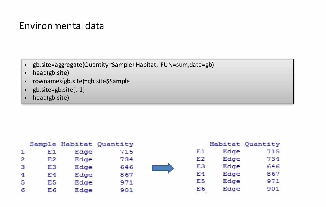
Environmentaldata
› gb.site=aggregate(Quantity~Sample+Habitat, FUN=sum,data=gb)› head(gb.site)› rownames(gb.site)=gb.site$Sample› gb.site=gb.site[,-1]› head(gb.site)
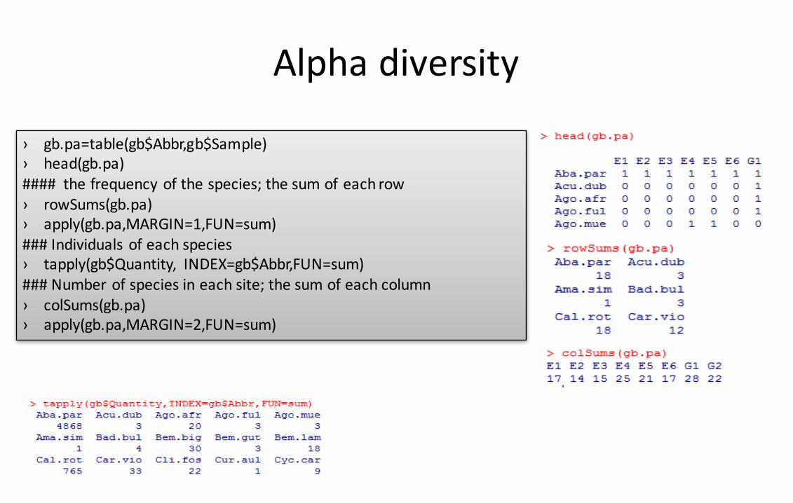
Alphadiversity
› gb.pa=table(gb$Abbr,gb$Sample)› head(gb.pa)####thefrequencyofthespecies;thesumofeachrow› rowSums(gb.pa)› apply(gb.pa,MARGIN=1,FUN=sum)###Individualsofeachspecies› tapply(gb$Quantity, INDEX=gb$Abbr,FUN=sum)###Numberofspeciesineachsite;thesumofeachcolumn› colSums(gb.pa)› apply(gb.pa,MARGIN=2,FUN=sum)

Alphadiversity
› library(vegan)› specnumber(gb.biol) ###speciesrichnessineachsite› length(specnumber(gb.biol,MARGIN=2)>0) ###speciesrichnessinallsites› diversity(gb.biol,”shannon”) ####Shannon-Winer diversityindex› diversity(gb.biol,”simpson”) ####Simpson diversityindex
E1 E3 E5 G1 G3 G5 W1 W3 W5
05
1015
2025
barplot(specnumber(gb.biol))
E1 E3 E5 G1 G3 G5 W1 W3 W5
0.0
0.5
1.0
1.5
2.0
barplot(diversity(gb.biol),col=“red”)
Veganpackage
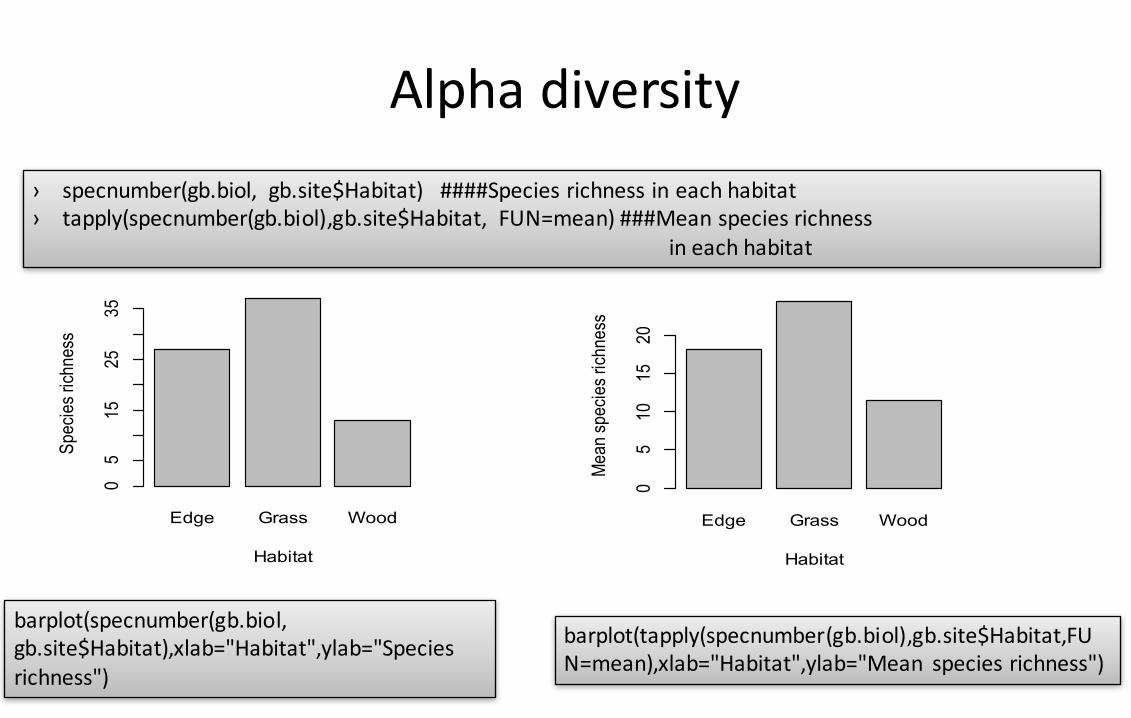
Alphadiversity› specnumber(gb.biol, gb.site$Habitat)####Speciesrichnessineachhabitat› tapply(specnumber(gb.biol),gb.site$Habitat, FUN=mean)###Meanspeciesrichness
ineachhabitat
Edge Grass Wood
Habitat
Spec
ies r
ichne
ss
05
1525
35
barplot(specnumber(gb.biol,gb.site$Habitat),xlab="Habitat",ylab="Speciesrichness")
Edge Grass Wood
Habitat
Mea
n sp
ecie
s rich
ness
05
1015
20barplot(tapply(specnumber(gb.biol),gb.site$Habitat,FUN=mean),xlab="Habitat",ylab="Mean speciesrichness")
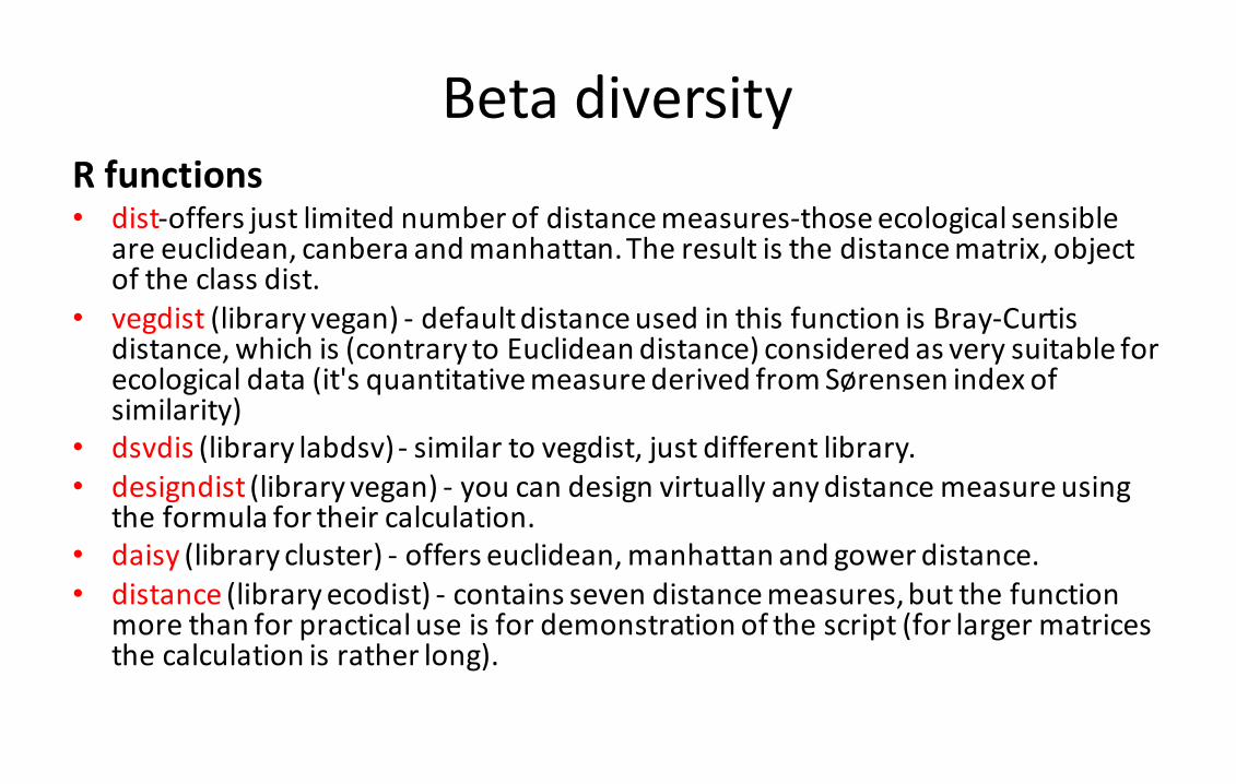
BetadiversityRfunctions• dist-offersjustlimitednumberofdistancemeasures-thoseecologicalsensible
areeuclidean,canbera andmanhattan.Theresultisthedistancematrix,objectoftheclassdist.
• vegdist (libraryvegan)- defaultdistanceusedinthisfunctionisBray-Curtisdistance,whichis(contrarytoEuclideandistance)consideredasverysuitableforecologicaldata(it'squantitativemeasurederivedfromSørensen indexofsimilarity)
• dsvdis (librarylabdsv)- similartovegdist,justdifferentlibrary.• designdist (libraryvegan)- youcandesignvirtuallyanydistancemeasureusing
theformulafortheircalculation.• daisy (librarycluster)- offerseuclidean,manhattan andgower distance.• distance (libraryecodist)- containssevendistancemeasures,butthefunction
morethanforpracticaluseisfordemonstrationofthescript(forlargermatricesthecalculationisratherlong).
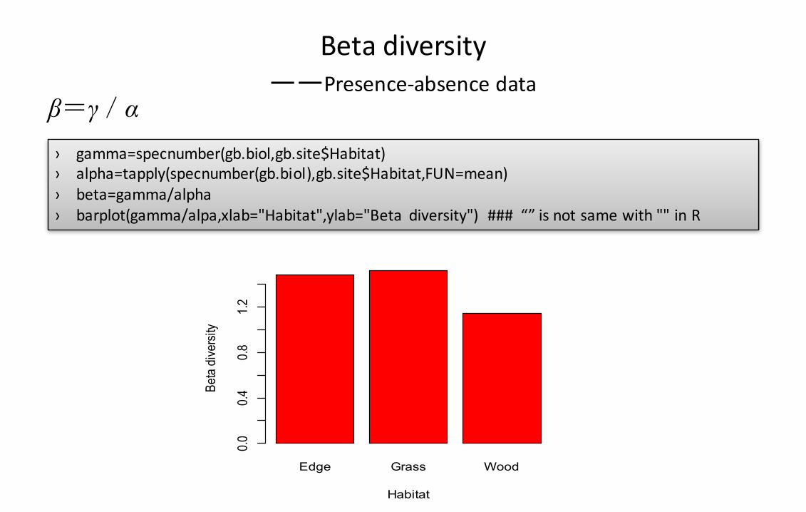
Betadiversity——Presence-absencedata
› gamma=specnumber(gb.biol,gb.site$Habitat)› alpha=tapply(specnumber(gb.biol),gb.site$Habitat,FUN=mean)› beta=gamma/alpha› barplot(gamma/alpa,xlab="Habitat",ylab="Beta diversity") ###“”isnotsamewith""inR
Edge Grass Wood
Habitat
Beta
dive
rsity
0.0
0.4
0.8
1.2
β=γ/α
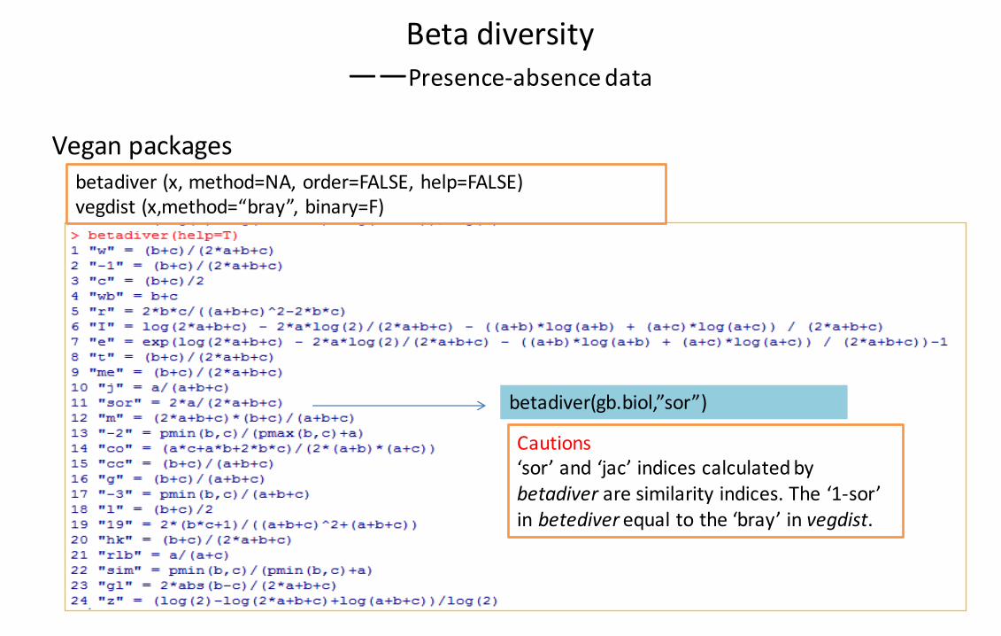
Betadiversity——Presence-absencedata
Veganpackagesbetadiver (x,method=NA,order=FALSE,help=FALSE)vegdist (x,method=“bray”,binary=F)
betadiver(gb.biol,”sor”)
Cautions‘sor’and‘jac’indicescalculatedbybetadiver aresimilarityindices.The‘1-sor’inbetediver equaltothe‘bray’invegdist.

Visualising betadiversityClusterdendrogram
› gb.beta=betadiver(gb.biol,method="w")› gb.clus=hclust(gb.beta)› plot(gb.clus,hang=-1,main="Beta
diversity",ylab="Betavalues",xlab="Bettlecommunity sample", sub="Complete joiningcluster")
W3
W6
W4
W5
W1
W2 G3 G2 G4 G1 G5 G6 E4 E5 E6 E1 E2 E3
0.0
0.2
0.4
0.6
Beta diversity
Complete joining clusterBettle community sample
Beta
valu
es
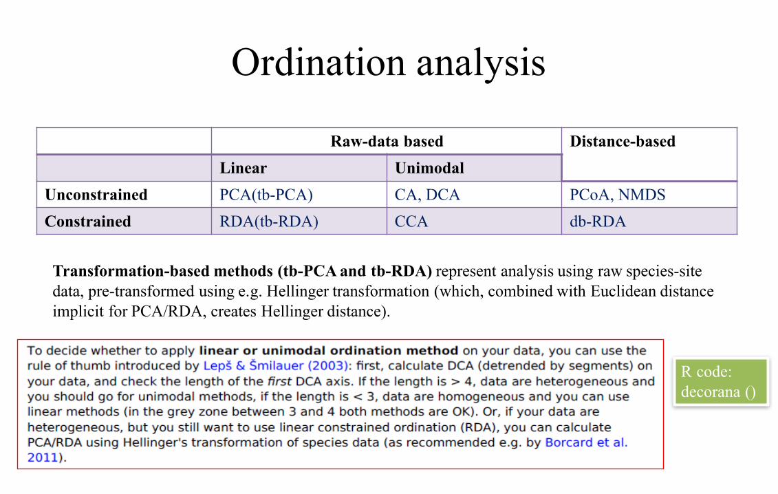
Ordination analysis
Raw-data based Distance-basedLinear Unimodal
Unconstrained PCA(tb-PCA) CA, DCA PCoA, NMDSConstrained RDA(tb-RDA) CCA db-RDA
Transformation-based methods (tb-PCA and tb-RDA) represent analysis using raw species-site data, pre-transformed using e.g. Hellinger transformation (which, combined with Euclidean distance implicit for PCA/RDA, creates Hellinger distance).
R code:decorana ()
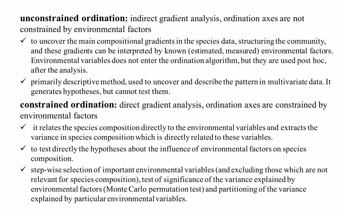
unconstrained ordination: indirect gradient analysis, ordination axes are not constrained by environmental factorsü to uncover the main compositional gradients in the species data, structuring the community,
and these gradients can be interpreted by known (estimated, measured) environmental factors. Environmental variables does not enter the ordination algorithm, but they are used post hoc, after the analysis.
ü primarily descriptive method, used to uncover and describe the pattern in multivariate data. It generates hypotheses, but cannot test them.
constrained ordination: direct gradient analysis, ordination axes are constrained by environmental factorsü it relates the species composition directly to the environmental variables and extracts the
variance in species composition which is directly related to these variables. ü to test directly the hypotheses about the influence of environmental factors on species
composition. ü step-wise selection of important environmental variables (and excluding those which are not
relevant for species composition), test of significance of the variance explained by environmental factors (Monte Carlo permutation test) and partitioning of the variance explained by particular environmental variables.
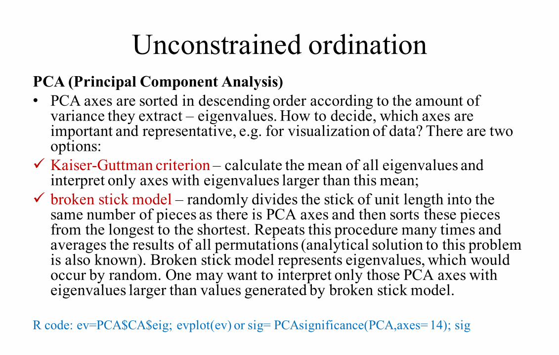
Unconstrained ordinationPCA (Principal Component Analysis)• PCA axes are sorted in descending order according to the amount of
variance they extract – eigenvalues. How to decide, which axes are important and representative, e.g. for visualization of data? There are two options:
ü Kaiser-Guttman criterion – calculate the mean of all eigenvalues and interpret only axes with eigenvalues larger than this mean;
ü broken stick model – randomly divides the stick of unit length into the same number of pieces as there is PCA axes and then sorts these pieces from the longest to the shortest. Repeats this procedure many times and averages the results of all permutations (analytical solution to this problem is also known). Broken stick model represents eigenvalues, which would occur by random. One may want to interpret only those PCA axes with eigenvalues larger than values generated by broken stick model.
R code: ev=PCA$CA$eig; evplot(ev) or sig= PCAsignificance(PCA,axes= 14); sig
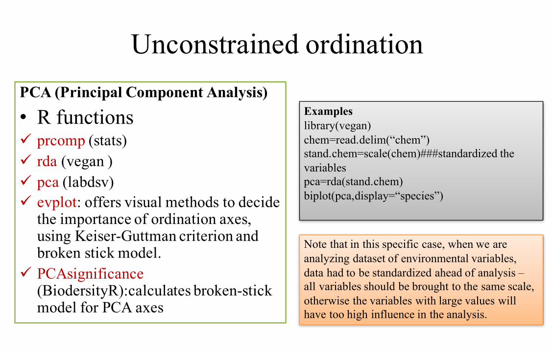
Unconstrained ordinationPCA (Principal Component Analysis)
• R functionsü prcomp (stats)ü rda (vegan )ü pca (labdsv)ü evplot: offers visual methods to decide
the importance of ordination axes, using Keiser-Guttman criterion and broken stick model.
ü PCAsignificance(BiodersityR):calculates broken-stick model for PCA axes
Exampleslibrary(vegan)chem=read.delim(“chem”)stand.chem=scale(chem)###standardized the variablespca=rda(stand.chem)biplot(pca,display=“species”)
Note that in this specific case, when we are analyzing dataset of environmental variables, data had to be standardized ahead of analysis –all variables should be brought to the same scale, otherwise the variables with large values will have too high influence in the analysis.
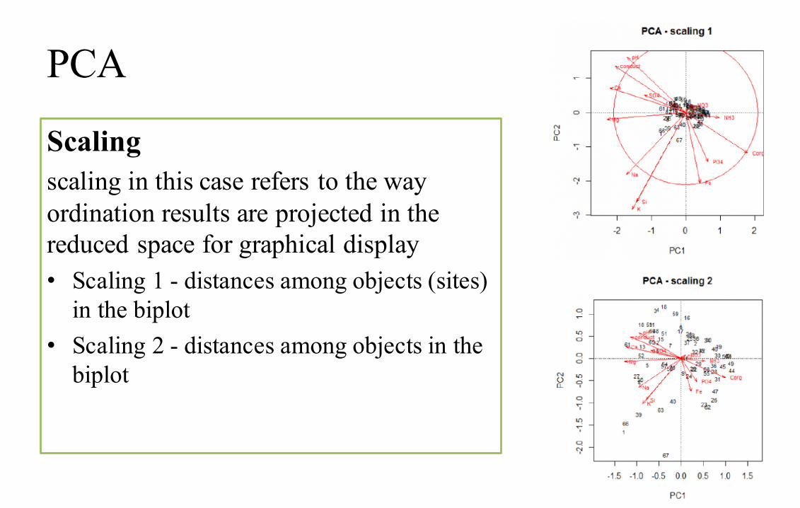
PCA
Scalingscaling in this case refers to the way ordination results are projected in the reduced space for graphical display• Scaling 1 - distances among objects (sites)
in the biplot• Scaling 2 - distances among objects in the
biplot

Unconstrained ordination
CA (Correspondence Analysis)ü Unimodal method of unconstrained ordinationü Suffers from artefact called arch effect, which is caused by non-linear
correlation between first and higher axesü Popular, even though clumsy way how to remove this artefact is to use
detrending in DCA.
R code:library(vegan)CA<-cca(sp)Ordiplot(CA)
Unconstrained ordination
DCA (Detrended Correspondence Analysis)
ü Detrended version of Correspondence Analysis, removing the arch effect from ordination
ü the length of the first axis (in SD units) refers to the heterogeneity or homogeneity of the dataset (a sort of beta diversity measure)
R code:library(vegan)DCA<-decorana(sp)

Unconstrained ordination
PCoA (Principal Coordinate Analysis)
ü This method is also known as MDS (Metric Multidimensional Scaling)ü PCA preserves Euclidean distances among samples and CA chi-square
distances, PCoA provides Euclidean representation of a set of objects whose relationship is measured by any similarity or distance measure chosen by the user
› pcoa(D, correction="none", rn=NULL)› D: A distance matrix of class dist or matrix› Correction: Correction methods for negative eigenvalues: "lingoes" and
"cailliez". Default value: "none".
Unconstrained ordination
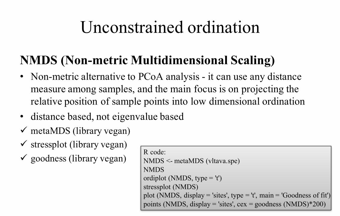
NMDS (Non-metric Multidimensional Scaling)• Non-metric alternative to PCoA analysis - it can use any distance
measure among samples, and the main focus is on projecting the relative position of sample points into low dimensional ordination
• distance based, not eigenvalue basedü metaMDS (library vegan)ü stressplot (library vegan)ü goodness (library vegan)
R code:NMDS <- metaMDS (vltava.spe)NMDSordiplot (NMDS, type = 't')stressplot (NMDS)plot (NMDS, display = 'sites', type = 't', main = 'Goodness of fit')points (NMDS, display = 'sites', cex = goodness (NMDS)*200)
Unconstrained ordination
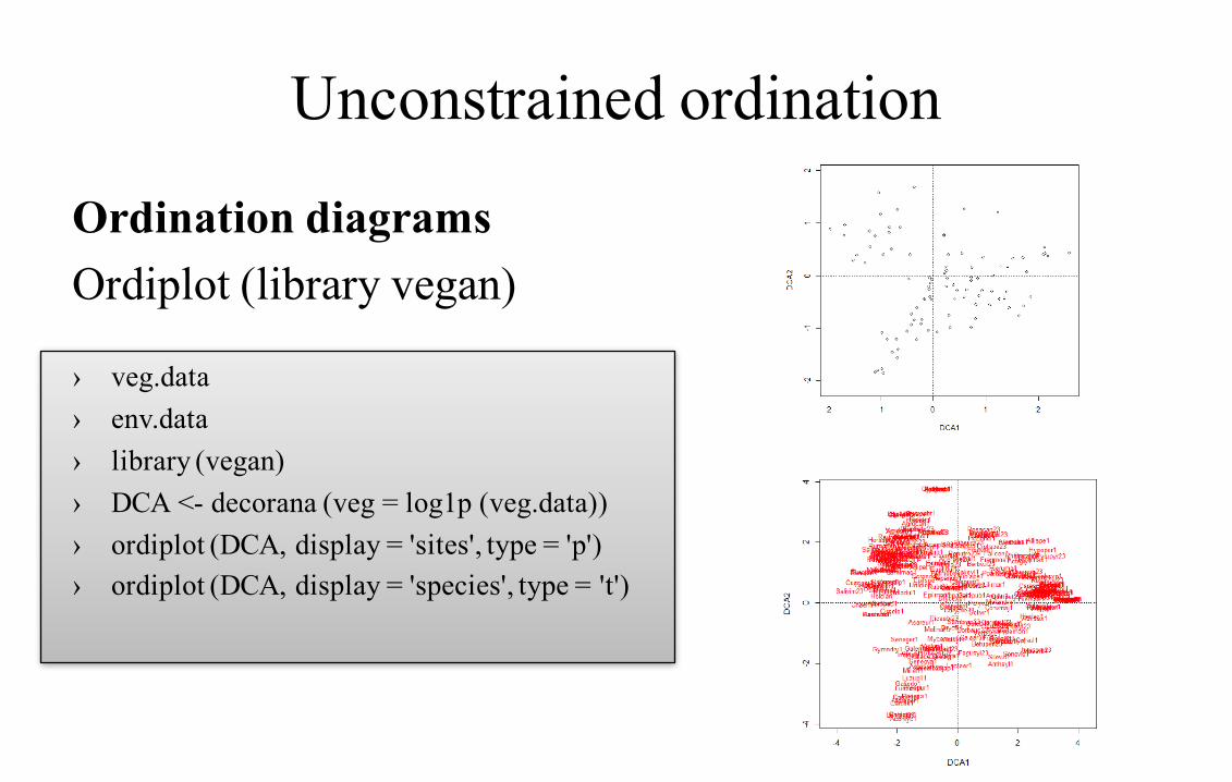
Ordination diagramsOrdiplot (library vegan)
› veg.data› env.data› library (vegan)› DCA <- decorana (veg = log1p (veg.data))› ordiplot (DCA, display = 'sites', type = 'p')› ordiplot (DCA, display = 'species', type = 't')
Unconstrained ordination
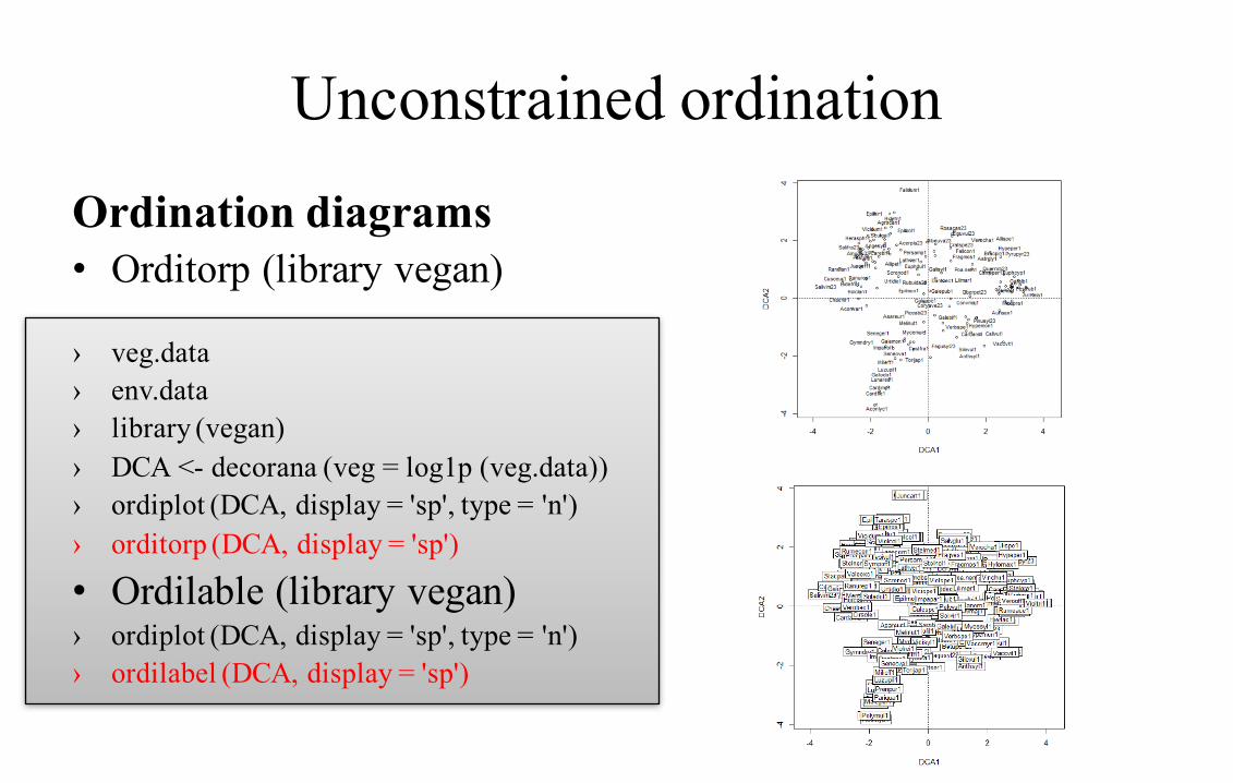
Ordination diagrams• Orditorp (library vegan)
› veg.data› env.data› library (vegan)› DCA <- decorana (veg = log1p (veg.data))› ordiplot (DCA, display = 'sp', type = 'n')› orditorp (DCA, display = 'sp')
• Ordilable (library vegan)› ordiplot (DCA, display = 'sp', type = 'n')› ordilabel (DCA, display = 'sp')
Unconstrained ordination
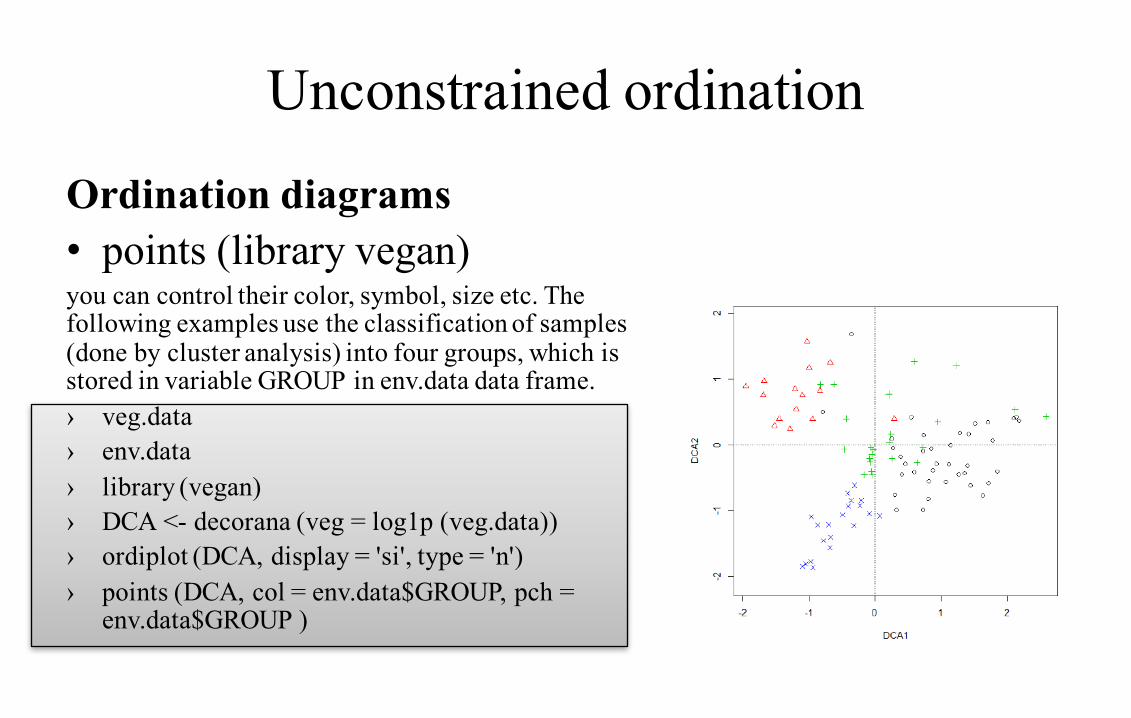
Ordination diagrams• points (library vegan)you can control their color, symbol, size etc. The following examples use the classification of samples (done by cluster analysis) into four groups, which is stored in variable GROUP in env.data data frame.› veg.data› env.data› library (vegan)› DCA <- decorana (veg = log1p (veg.data))› ordiplot (DCA, display = 'si', type = 'n')› points (DCA, col = env.data$GROUP, pch =
env.data$GROUP )
Unconstrained ordination
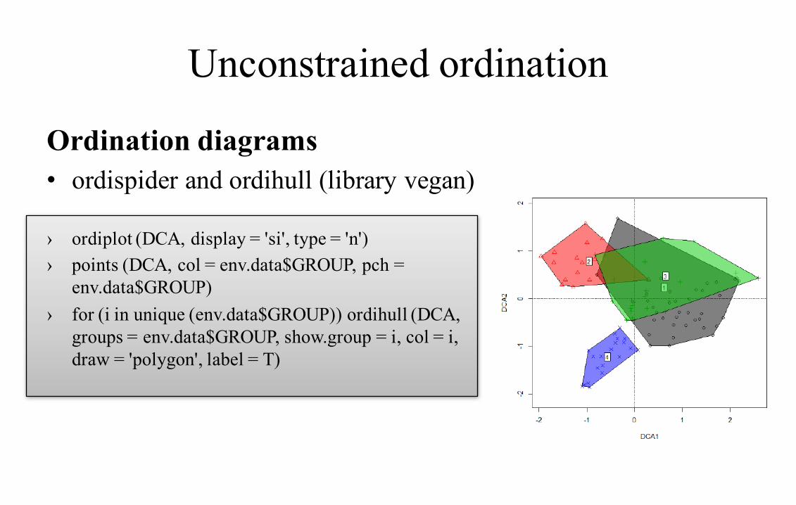
Ordination diagrams• ordispider and ordihull (library vegan)
› ordiplot (DCA, display = 'si', type = 'n')› points (DCA, col = env.data$GROUP, pch =
env.data$GROUP)› for (i in unique (env.data$GROUP)) ordihull (DCA,
groups = env.data$GROUP, show.group = i, col = i, draw = 'polygon', label = T)
Unconstrained ordination
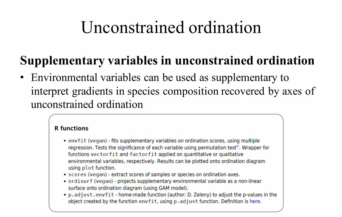
Supplementary variables in unconstrained ordination• Environmental variables can be used as supplementary to
interpret gradients in species composition recovered by axes of unconstrained ordination
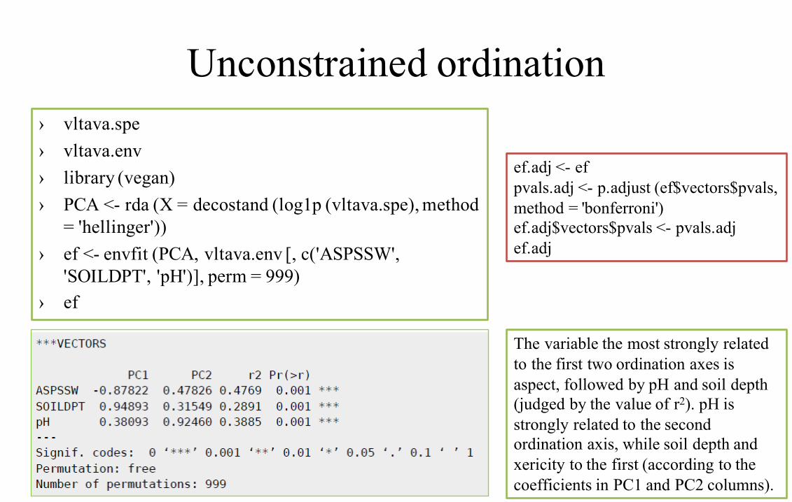
Unconstrained ordination› vltava.spe› vltava.env› library (vegan)› PCA <- rda (X = decostand (log1p (vltava.spe), method
= 'hellinger'))› ef <- envfit (PCA, vltava.env [, c('ASPSSW',
'SOILDPT', 'pH')], perm = 999)› ef
The variable the most strongly related to the first two ordination axes is aspect, followed by pH and soil depth (judged by the value of r2). pH is strongly related to the second ordination axis, while soil depth and xericity to the first (according to the coefficients in PC1 and PC2 columns).
ef.adj <- efpvals.adj <- p.adjust (ef$vectors$pvals, method = 'bonferroni')ef.adj$vectors$pvals <- pvals.adjef.adj
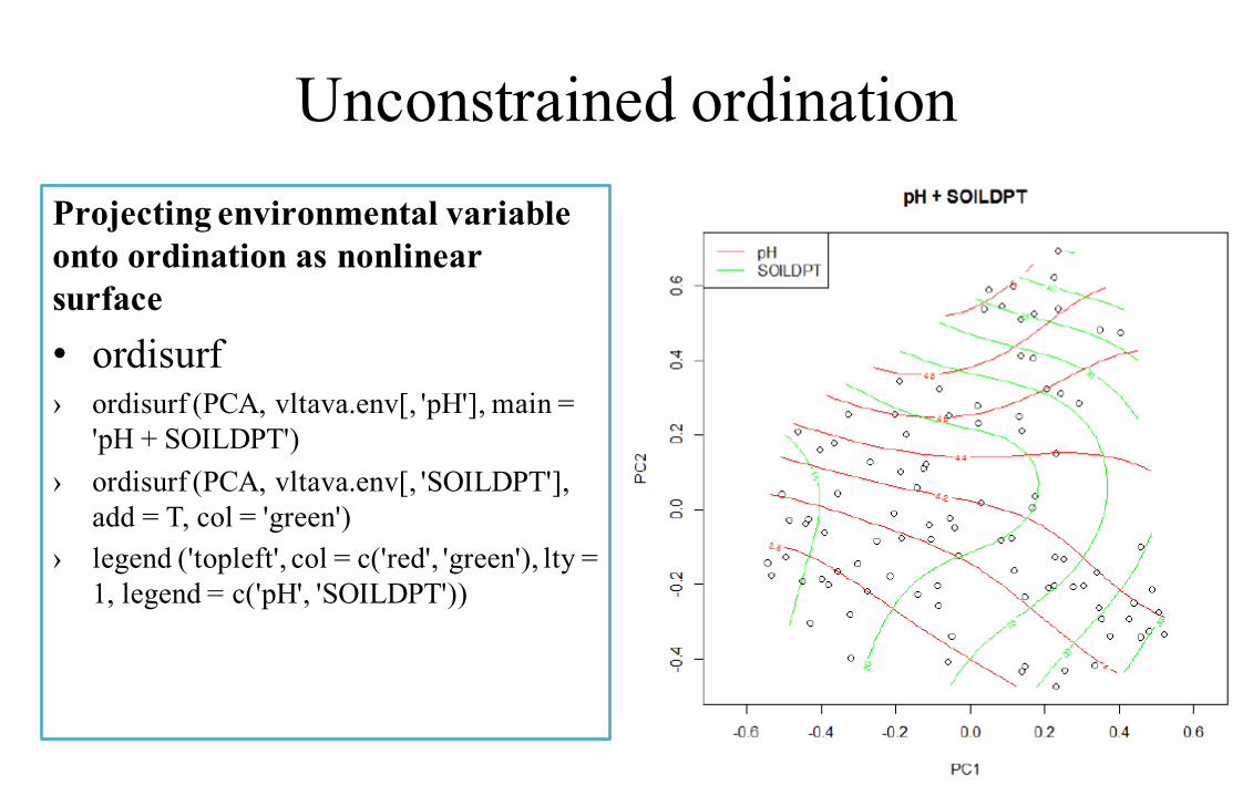
Unconstrained ordinationProjecting environmental variable onto ordination as nonlinear surface• ordisurf› ordisurf (PCA, vltava.env[, 'pH'], main =
'pH + SOILDPT')› ordisurf (PCA, vltava.env[, 'SOILDPT'],
add = T, col = 'green')› legend ('topleft', col = c('red', 'green'), lty =
1, legend = c('pH', 'SOILDPT'))
Unconstrained ordination• Use of mean Ellenberg indicator values as supplementary variables

Constrained ordination
RDA (Redundancy Analysis)• matrix syntaxü RDA = rda (Y, X, W)ü where Y is the response matrix (species composition), X is the explanatory
matrix (environmental factors) and W is the matrix of covariables• formula syntaxü RDA = rda (Y ~ var1 + factorA + var2*var3 + Condition (var4), data = XW)ü as explanatory are used: quantitative variable var1, categorical variable
factorA, interaction term between var2 and var3, whereas var4 is used as covariable and hence partialled out.
Constrained ordination
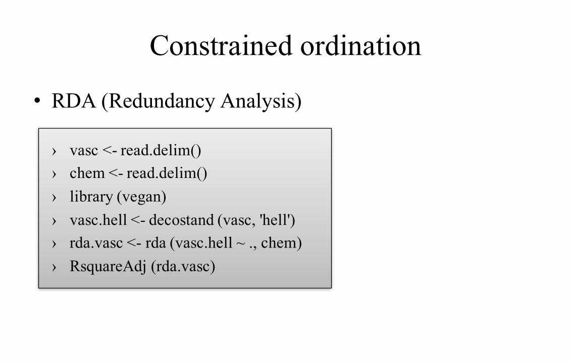
• RDA (Redundancy Analysis)
› vasc <- read.delim()› chem <- read.delim()› library (vegan)› vasc.hell <- decostand (vasc, 'hell')› rda.vasc <- rda (vasc.hell ~ ., chem)› RsquareAdj (rda.vasc)
Constrained ordination
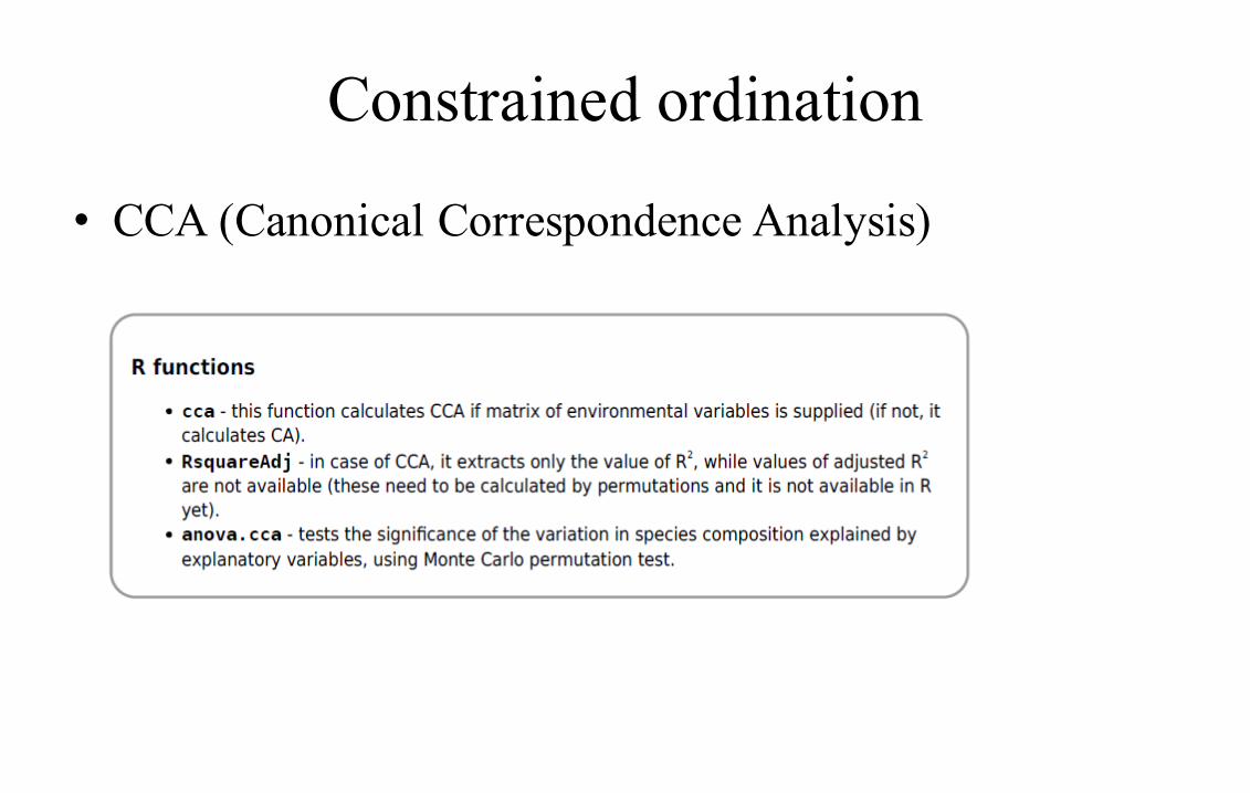
• CCA (Canonical Correspondence Analysis)
Constrained ordination
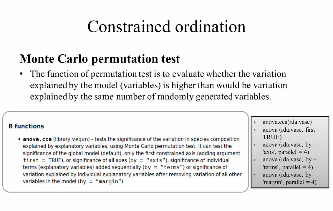
Monte Carlo permutation test• The function of permutation test is to evaluate whether the variation
explained by the model (variables) is higher than would be variation explained by the same number of randomly generated variables.
› anova.cca(rda.vasc)› anova (rda.vasc, first =
TRUE)› anova (rda.vasc, by =
'axis', parallel = 4)› anova (rda.vasc, by =
'terms', parallel = 4)› anova (rda.vasc, by =
'margin', parallel = 4)
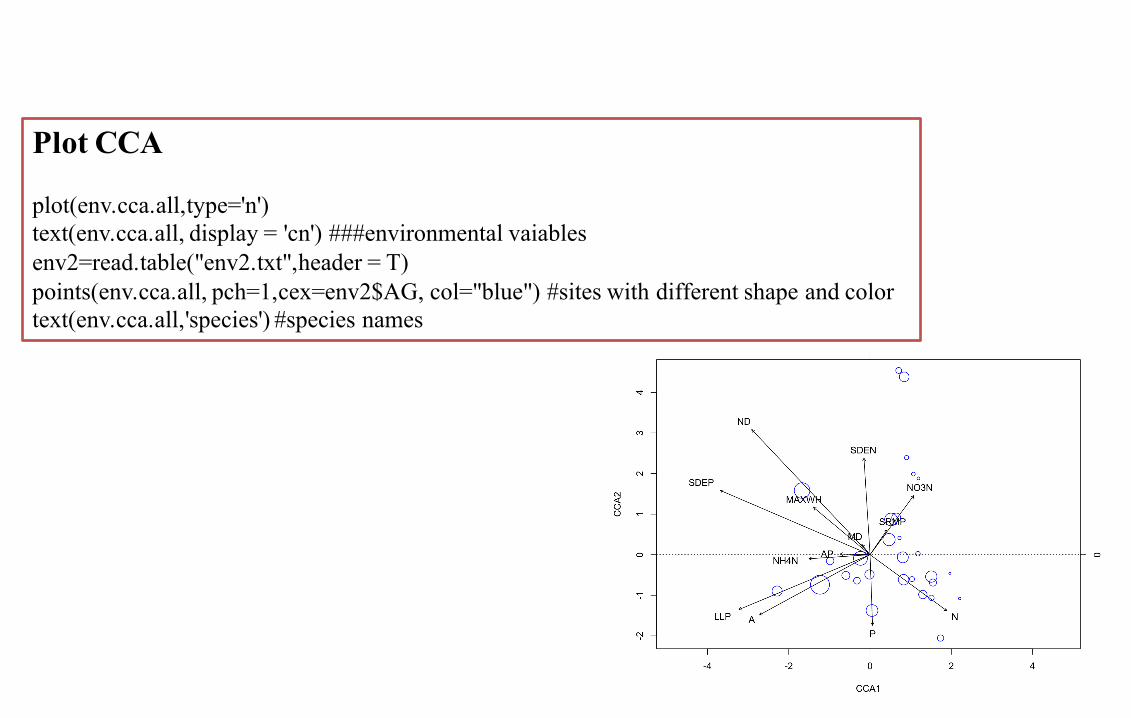
Plot CCA
plot(env.cca.all,type='n')text(env.cca.all, display = 'cn') ###environmental vaiablesenv2=read.table("env2.txt",header = T)points(env.cca.all, pch=1,cex=env2$AG, col="blue") #sites with different shape and colortext(env.cca.all,'species') #species names
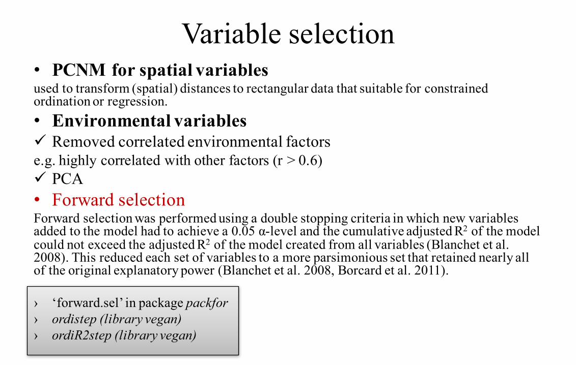
Variable selection• PCNM for spatial variablesused to transform (spatial) distances to rectangular data that suitable for constrained ordination or regression.• Environmental variablesü Removed correlated environmental factorse.g. highly correlated with other factors (r > 0.6)ü PCA• Forward selectionForward selection was performed using a double stopping criteria in which new variables added to the model had to achieve a 0.05 α-level and the cumulative adjusted R2 of the model could not exceed the adjusted R2 of the model created from all variables (Blanchet et al. 2008). This reduced each set of variables to a more parsimonious set that retained nearly all of the original explanatory power (Blanchet et al. 2008, Borcard et al. 2011).
› ‘forward.sel’ in package packfor› ordistep (library vegan)› ordiR2step (library vegan)

PCNM• The PCNM functions are used to express distances in rectangular form that
is similar to normal explanatory variables used in, e.g., constrained ordination (rda, cca and capscale) or univariate regression (lm) together with environmental variables
• This is regarded as a more powerful method than forcing rectangular environmental data into distances and using them in partial mantel analysis (mantel.partial) together with geographic distances
• R code: pcnm() in vegan› pcnm(GeoDist)› pcnm(GeoDist)$vectors

Forward selectionforward.sel(Y, X, K = nrow(X) – 1, …)• Y: A matrix of n lines and m columns that contains (numeric) response variable• X: A matrix of n lines and p columns that contains (numeric) explanatory
variables.
› library(packfor)› library(picante)› forward.sel(pcoa(Beta.bray)$vectors,pcnm(GeoDist)$vectors) ###› forward.sel(pcoa(Beta.bray)$vectors,Env[,1:7])
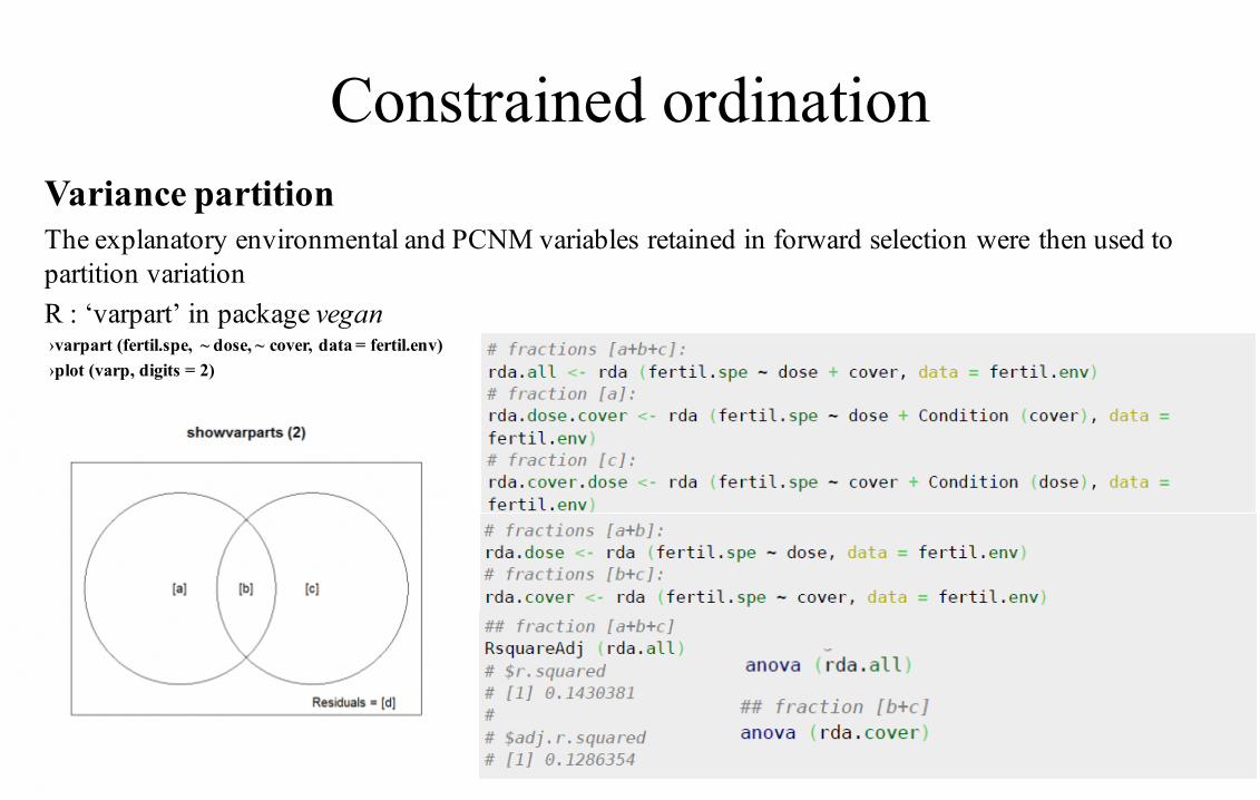
Constrained ordinationVariance partitionThe explanatory environmental and PCNM variables retained in forward selection were then used to partition variationR : ‘varpart’ in package vegan›varpart (fertil.spe, ~ dose, ~ cover, data = fertil.env)›plot (varp, digits = 2)
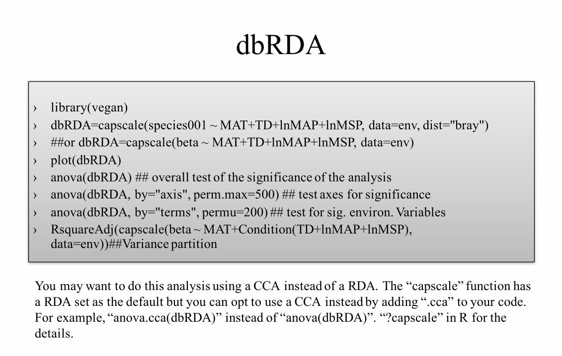
dbRDA
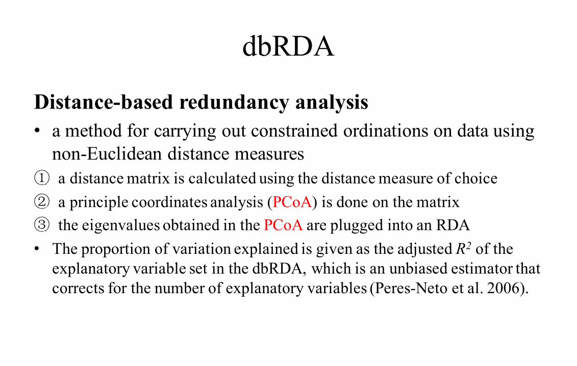
Distance-based redundancy analysis• a method for carrying out constrained ordinations on data using
non-Euclidean distance measures① a distance matrix is calculated using the distance measure of choice② a principle coordinates analysis (PCoA) is done on the matrix③ the eigenvalues obtained in the PCoA are plugged into an RDA• The proportion of variation explained is given as the adjusted R2 of the
explanatory variable set in the dbRDA, which is an unbiased estimator that corrects for the number of explanatory variables (Peres-Neto et al. 2006).
dbRDA
› library(vegan)› dbRDA=capscale(species001 ~ MAT+TD+lnMAP+lnMSP, data=env, dist="bray")› ##or dbRDA=capscale(beta ~ MAT+TD+lnMAP+lnMSP, data=env)› plot(dbRDA)› anova(dbRDA) ## overall test of the significance of the analysis› anova(dbRDA, by="axis", perm.max=500) ## test axes for significance› anova(dbRDA, by="terms", permu=200) ## test for sig. environ. Variables› RsquareAdj(capscale(beta ~ MAT+Condition(TD+lnMAP+lnMSP),
data=env))##Variance partition
You may want to do this analysis using a CCA instead of a RDA. The “capscale” function has a RDA set as the default but you can opt to use a CCA instead by adding “.cca” to your code. For example, “anova.cca(dbRDA)” instead of “anova(dbRDA)”. “?capscale” in R for the details.
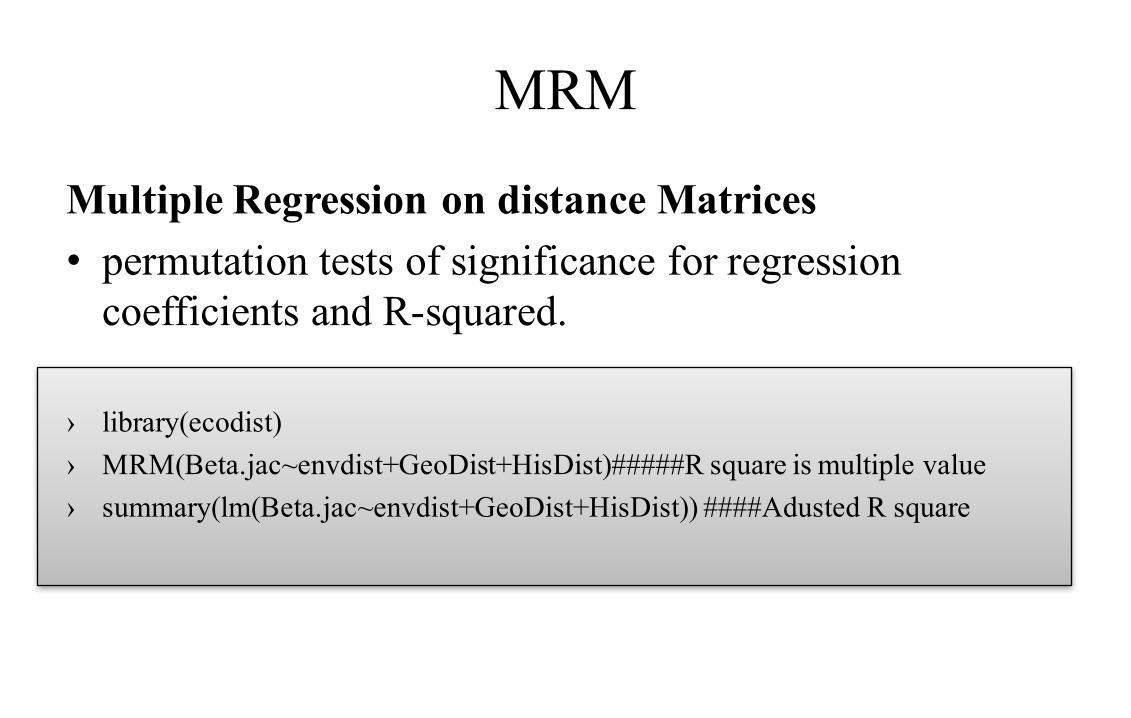
MRM
Multiple Regression on distance Matrices• permutation tests of significance for regression
coefficients and R-squared.
› library(ecodist)› MRM(Beta.jac~envdist+GeoDist+HisDist)#####R square is multiple value› summary(lm(Beta.jac~envdist+GeoDist+HisDist)) ####Adusted R square
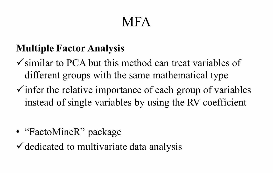
MFA
Multiple Factor Analysisüsimilar to PCA but this method can treat variables of
different groups with the same mathematical typeüinfer the relative importance of each group of variables
instead of single variables by using the RV coefficient
• “FactoMineR” packageüdedicated to multivariate data analysis
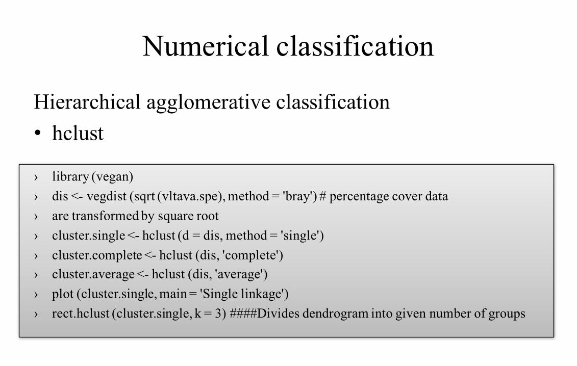
Numerical classification
Hierarchical agglomerative classification• hclust
› library (vegan)› dis <- vegdist (sqrt (vltava.spe), method = 'bray') # percentage cover data› are transformed by square root› cluster.single <- hclust (d = dis, method = 'single')› cluster.complete <- hclust (dis, 'complete')› cluster.average <- hclust (dis, 'average')› plot (cluster.single, main = 'Single linkage')› rect.hclust (cluster.single, k = 3) ####Divides dendrogram into given number of groups
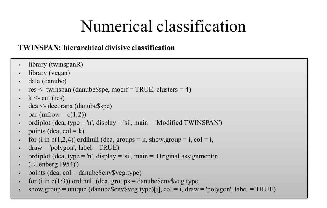
Numerical classificationTWINSPAN: hierarchical divisive classification
› library (twinspanR)› library (vegan)› data (danube)› res <- twinspan (danube$spe, modif = TRUE, clusters = 4)› k <- cut (res)› dca <- decorana (danube$spe)› par (mfrow = c(1,2))› ordiplot (dca, type = 'n', display = 'si', main = 'Modified TWINSPAN')› points (dca, col = k)› for (i in c(1,2,4)) ordihull (dca, groups = k, show.group = i, col = i,› draw = 'polygon', label = TRUE)› ordiplot (dca, type = 'n', display = 'si', main = 'Original assignment\n› (Ellenberg 1954)')› points (dca, col = danube$env$veg.type)› for (i in c(1:3)) ordihull (dca, groups = danube$env$veg.type,› show.group = unique (danube$env$veg.type)[i], col = i, draw = 'polygon', label = TRUE)
References• David Zelený. Analysis of community ecology data in R
http://www.davidzeleny.net/anadat-r/• Mark Gardener. Community Ecology: Analytical Methods Using R and Excel• Borcard D., Gillet G., Legendre P. Numerical Ecology with R