arxiv.org · 2017-09-12 · 2 S. GADAT, F. PANLOUP stochastic algorithm (θn)n≥0 deﬁned by: θ0 ∈ Rd and (1.1) ∀n≥ 0, θn+1 = θn −γn+1Λ(θn,Zn+1), where (γn)n≥1

arX

iv:1

709.

0334

2v1

[m

ath.

ST]

11

Sep

2017

arXiv: arXiv:0000.0000

OPTIMAL NON-ASYMPTOTIC BOUND OF THERUPPERT-POLYAK AVERAGING WITHOUT STRONG

CONVEXITY

By Sebastien Gadat and Fabien Panloup

Toulouse School of Economics, University of Toulouse I CapitoleLaboratoire Angevin de Recherche en Mathematiques, Universite d’Angers

This paper is devoted to the non-asymptotic control of the mean-squared error for the Ruppert-Polyak stochastic averaged gradient de-scent introduced in the seminal contributions of [Rup88] and [PJ92].In our main results, we establish non-asymptotic tight bounds (opti-mal with respect to the Cramer-Rao lower bound) in a very generalframework that includes the uniformly strongly convex case as wellas the one where the function f to be minimized satisfies a weakerKurdyka- Lojiasewicz-type condition [Loj63, Kur98]. In particular, itmakes it possible to recover some pathological examples such as on-line learning for logistic regression (see [Bac14]) and recursive quan-tile estimation (an even non-convex situation). Finally, our bound isoptimal when the decreasing step (γn)n≥1 satisfies: γn = γn−β withβ = 3/4, leading to a second-order term in O(n−5/4).

1. Introduction.

1.1. Averaging principle for stochastic algorithms.

Initial averaging algorithm. Let f : Rd → R be a function that belongs

to C2(Rd,R), i.e., the space of twice differentiable functions from Rd to R

with continuous second partial derivatives. Let us assume that ∇f admitsthe following representation: a measurable function Λ : Rd × R

p → Rd and

a random variable Z with values in Rp exist such that Z is distributed

according to µ such that:

∀θ ∈ Rd, ∇f(θ) = E[Λ(θ, Z)].

In this case, the Robbins-Monro procedure introduced in the seminal con-tribution [RM51] is built with an i.i.d. sequence of observations (Zi)i≥1

distributed according to µ. It is well known that under appropriate as-sumptions, the minimizers of f can be approximated through the recursive

AMS 2000 subject classifications: Primary 62L20, 80M50; secondary 68W25Keywords and phrases: stochastic algorithms, optimization, averaging

1

http://arxiv.org/abs/1709.03342v1

http://arxiv.org/abs/arXiv:0000.0000

2 S. GADAT, F. PANLOUP

stochastic algorithm (θn)n≥0 defined by: θ0 ∈ Rd and

(1.1) ∀n ≥ 0, θn+1 = θn − γn+1Λ(θn, Zn+1),

where (γn)n≥1 denotes a non-increasing sequence of positive numbers suchthat:

Γn :=n∑

k=1

γkn−→+∞−−−−−→ +∞ and γn

n−→+∞−−−−−→ 0.

The standard averaging procedure of Ruppert-Polyak (referred to as RPaveraging) consists in introducing a Cesaro average over the iterations ofthe Robbins-Monro sequence defined by:

θn =1

n

n∑

k=1

θk, n ≥ 1.

It is well known that such an averaging procedure is a way to improve theconvergence properties of the original algorithm (θn)n≥1 by minimizing theasymptotic variance induced by the algorithm. More precisely, when f isa strongly convex function and possesses a unique minimum θ⋆, (θn)n≥1,√n(θn − θ⋆)n≥1 converges in distribution to a Gaussian law whose variance

attains the Cramer-Rao lower bound of any (oracle) unbiased estimation ofθ⋆ (see Theorem 1 for a precise statement of this state of the art result).Such results are generally achieved asymptotically in general situations wheref is assumed to be strongly convex, we refer to [PJ92] for the initial asymp-totic description and to [For15] for some more general results. In [BM11], anon-asymptotic optimal (with a sharp first order term) result is obtained inthe strongly convex situation under restrictive moment assumptions on thenoisy gradients. It is also dealt with non asymptotically without sharp con-stants in some specific cases where such a strong convexity property fails(on-line logistic regression [Bac14], recursive median estimation [CCZ13,CCGB17] for example). Nevertheless, a general result for strongly convexor not situations under some mild conditions on the noise while preservinga sharp optimal O(n−1) rate of convergence of the L

2-risk is yet missing.In this paper, our purpose is to derive a sharp study on the L

2-risk ofthe averaged process (θn)n≥0 and derive an optimal variance result, whichdepends on the Hessian of f at θ⋆ without restricting ourself to the stronglyconvex or even convex case. To do so, we will introduce a weak assumption onf that generalizes a global Kurdyka- Lojasiewicz inequality assumption on f(see [Loj63, Kur98]). We are also interested in the adaptivity of (θn)n≥0: theability of the algorithm to behave optimally and independently on the localvalue of the Hessian of f at θ⋆. We also alleviate the convexity conditionson f under which such bounds can be achieved.

NON-ASYMPTOTIC ANALYSIS OF THE RUPPERT-POLYAK AVERAGING 3

1.2. Polyak-Juditsky central limit theorem. To assess the quality of a non-asymptotic control of the sequences (θn)n≥0, we recall the CLT associatedwith (θn)n≥0, whose statement is adapted from [PJ92]1 with the stronglyconvex assumption (HSC(α)) commonly used in the optimization commu-nity:

Assumption HSC(α) - Strongly convex function f is a strongly convexfunction of parameter α > 0 in the set:

(1.2) SC(α) :=f ∈ C2(Rd) : D2f − αId ≥ 0

where D2f stands for the Hessian matrix of f and inequality A ≥ 0 for anymatrix A has to be understood in the sense of quadratic forms.The set SC(α) captures many practical situations such as the least squareoptimization problem in statistical linear models for example.

Theorem 1 ([PJ92]). Assume that:

i) the function f is in SC(α) and x 7−→ D2f(x) is bounded.

ii) γnn→+∞−−−−−→ 0 and γ−1

n (γn − γn+1) = o+∞(γn),iii) the convergence in probability of the conditional covariance holds, i.e.,

limn−→+∞

E[∆Mn+1∆MTn+1|Fn] = S⋆,

then √n(θn − θ⋆)

L,n−→+∞−−−−−−−→ N (0,Σ⋆),

where

(1.3) Σ⋆ = D2f(θ⋆)−1S⋆D2f(θ⋆)−1.

Theorem 1 shows that the Ruppert-Polyak averaging produces an asymp-totically optimal algorithm whose rate of convergence is O(n−1), which isminimax optimal in the class of strongly convex stochastic minimizationproblems (see, e.g., [NY83]). Moreover, the asymptotic variance is also opti-mal because it attains the Cramer-Rao lower bound (see e.g. [PJ92, CB01]).It is also important to observe that (θn)n≥0 is an adaptive sequence sincethe previous result is obtained independently of the size of D2f(θ⋆) as soonas the sequence (γn)n≥1 is chosen as γn = γn−β with β ∈ (0, 1).

1In [PJ92], the result is stated in a slightly more general framework with the help of aLyapunov function. We have chosen to simplify the statement for the sake of readability.


1.3. Main results. As pointed out by many authors in some recent works(we refer to [BM11], [Bac14] and [CCZ13], among others), even though verygeneral, Theorem 1 has the usual drawback of being only asymptotic withrespect to n. To bypass this weak quantitative result, some improvementsare then obtained for various particular cases of minimization problems (e.g.,logistic regression, least square minimization, median and quantile estima-tions) in the literature.Below, we are interested in deriving some non-asymptotic inequality resultson the RP averaging for the minimization of f . We therefore establish somenon-asymptotic mean squared error upper bounds for (|θn − θ⋆|22)n≥1. Wealso investigate some more specific situations without any strong convexityproperty (quantile estimation and logistic regression). In each case, we areinterested in the first-order term of the limiting variance involved in Theorem1 (and in the Cramer-Rao lower bound as well).

1.3.1. Notations. The canonical filtration (Fn)n≥1 refers to the filtrationassociated with the past events before time n + 1: Fn = σ(θ1, . . . , θn) forany n ≥ 1. The conditional expectation at time n is then denoted by E[.|Fn].For any vector y ∈ R

d, yT denotes the transpose of y, whereas |y| is theEuclidean norm of y in R

d. The set Md(R) refers to the set of squared realmatrices of size d × d and the tensor product ⊗2 is used to refer to thefollowing quadratic form:

∀M ∈ Md(R) ∀y ∈ Rd My⊗2 = yTMy.

Id is the identity matrix in Md(R) and Od(R) denotes the set of orthonormalreal matrices of size d× d:

Od(R) :=Q ∈ Md(R) : QTQ = Id

.

Finally, the notation ‖ . ‖ corresponds to a (non-specified) norm on Md(R).For two positive sequences (an)n≥1 and (bn)n≥1, the notation an . bn refersto the domination relationship, i.e. an ≤ c bn where c is independent of n.The binary relationship an = O(bn) then holds if and only if |an| . |bn|.Finally, if for all n ∈ N, bn 6= 0, an = o(bn) if lim an

bn= 0 when n −→ +∞.

In the rest of the paper, we assume that f satisfies the following properties:

(1.4) lim|x|→+∞

f(x) = +∞ and x ∈ Rd,∇f(x) = 0 = θ⋆

where θ⋆ is thus the unique minimum of f . Without loss of generality, wealso assume that f(θ⋆) = 0.


We also consider the common choice for (γn)n≥1 (for γ > 0 and β ∈ (0, 1)):

∀n ≥ 1 γn = γn−β.

In particular, we have Γn ∼ γ1−βn

1−β −→ +∞ and γn −→ 0 as n −→ +∞.

The rest of this section is devoted to the statement of our main results. InSubsection 1.3.2, we state our main general result (Theorem 2) under somegeneral assumptions on the noise part and on the behavior of the Lp-normof the original procedure (θn)n≥1 ((Lp,

√γn)-consistency). Then, in the

next subsections, we provide some settings where this consistency conditionis satisfied: under a strong convexity assumption in Subsection 1.3.3 andunder a Kurdyka- Lojiasewicz-type assumption in Subsection 1.3.4.

1.3.2. Non asymptotic adaptive and optimal inequality. Our first main re-sult is Theorem 2 and we introduce the following definition.

Definition 1.1 ((Lp,√γn)-consistency). Let p > 0. We say that a sequence

(θn)n≥1 satisfies the (Lp,√γn)-consistency (convergence rate condition) if(

θn√γn

)n≥1

is bounded in Lp, i.e., if:

∃ cp > 0 ∀n ≥ 1 E|θn|p ≤ cpγnp2 .

Note that according to the Jensen inequality, the (Lp,√γn)-consistency im-

plies the (Lq,√γn)-consistency for any 0 < q < p. As mentioned before, this

definition refers to the behaviour of the crude procedure (θn)n≥1 definedby Equation (1.1). We will prove that Definition 1.1 is a key property toderive non-asymptotic bounds for the RP-averaged algorithm (θn)n≥1 (seeTheorem 2 below).

We also introduce a smoothness assumption on the covariance of the mar-tingale increment:

Assumption (HS) - Covariance of the martingale increment Thecovariance of the martingale increment satisfies:

∀θ ∈ Rd

E[∆Mn+1∆M

tn+1|Fn

]= S(θn) a.s.

where S : Rd → Md(R) is a Lipschitz continuous function:

∃L > 0 ∀(θ1, θ2) ∈ Rd ‖S(θ1) − S(θ2)‖ ≤ L|θ1 − θ2|.


When compared to Theorem 1, Assumption (HS) is more restrictive butin fact corresponds to the usual framework. Under additional technicalities,this assumption may be relaxed to a local Lipschitz behaviour of S. Forreasons of clarity, we preferred to reduce our purpose to this reasonablesetting.We now state our main general result:

Theorem 2 (Optimal non-asymptotic bound for the averaging procedure).Let γn = γn−β with β ∈ (1/2, 1). Assume that (θn)n≥1 is (L4,

√γn)-consistent

and that Assumption (HS) holds. Suppose moreover that D2f(θ⋆) is positive-definite.Then, a large enough C exists such that:

∀n ∈ N⋆

E

[|θn − θ⋆|2

]≤ Tr(Σ⋆)

n+ Cn−rβ ,

where Σ⋆ is defined in Equation (1.3) (with S⋆ = S(θ⋆)) and

rβ =

(β +

1

2

)∧ (2 − β) .

In particular, rβ > 1 for all β ∈ (1/2, 1) and β 7−→ rβ attains its maximumfor β = 3/4, which yields:

∀n ∈ N⋆

E

[|θn − θ⋆|2

]≤ Tr(Σ⋆)

n+ Cn−5/4.

The result stated by Theorem 2 deserves three main remarks.

• First, we obtain the exact optimal rate O(n−1) with the sharp constantTr(Σ⋆) as shown by Theorem 1. Hence, at the first order, Theorem 2 showsthat the averaging procedure is minimax optimal with respect to the Cramer-Rao lower bound. Moreover, the result is adaptive with respect to the valueof the Hessian D2f(θ⋆): any sequence γn = γn−β with β ∈ (1/2, 1) andγ > 0, regardless the value of β or γ, produces the result of Theorem 2.We should note that such an adaptive property does not hold for the initialsequence (θn)n≥1 as proved by the central limit theorem satisfied by (θn)n≥1

(see [Duf97] for example). To the best of our knowledge, such a result wasonly obtained in [BM11] for strongly convex objective functions.

• Second, Theorem 2 does not require any convexity assumptions on f .However, this formulation is misleading by itself since we instead assume a(Lp,

√γn)-consistency for the initial sequence (θn)n≥1. We will discuss how

we can guarantee such a property in Theorem 4 in convex situations or


in some more general cases. The conclusion of Theorem 2 holds as soonas (θn)n≥1 satisfies E[|θn − θ⋆|4] ≤ Cγn2, which permits us to efficientlylinearize the drift of the sequence (θn)n≥1.Our proof is quite different from the one of [BM11], which gives an optimalresult only in the strongly convex case, whereas the rate is seriously dam-aged in the non-strongly convex situation (Theorems 3 and 6 of [BM11]).In contrast, our result can also apply to some non-strongly convex objectivefunctions while preserving the optimal upper bound, and holds under muchweaker conditions on the noise setting. Our improvement is achieved througha spectral analysis of the second-order Markov chain induced by (θn)n≥1.This spectral analysis requires a preliminary linearization step of the driftfrom θn to θn+1. The cost of this linearization is absorbed by a preliminarycontrol of the initial sequence (θn)n≥1, (Lp,

√γn)-consistency for p = 4 (see

Proposition 1.1 and Theorem 3 for results on the (Lp,√γn)-consistency).

Note that this (Lp,√γn)-consistency for p = 4 is also a property used in

[CCGB17] and [BM11].• Finally, we prove that the second order term is O(n−rβ) and that its sizeis minimized according to the choice β = 3/4. With this optimal calibrationof β, the size of the second-order term is n−5/4 in the general case. (Asmentioned in Remark 2.2, this bound can be improved if the third derivativeof f vanishes in θ⋆. In the literature, several choices for the value of βhave been proposed. In the particular case of the recursive quantile problem(see e.g. [CCGB17]), the authors suggest to use β = 2/3 to minimize thesecond-order terms without any explicit quantitative result. For stronglyconvex functions, it is indicated in [BM11] to also use β = 2/3 and thesecond order term obtained in [BM11] is n−7/6, which is larger than n−5/4.Even though the second-order terms are of marginal importance, Theorem2 provides stronger results than Theorem 3 of [BM11] and results stated in[CCZ13, CCGB17]. It also appears that the condition β > 1/2 and β < 1 isnecessary to obtain the tight constant Tr(Σ⋆), and the choice β = 1/2 doesnot seem appropriate in a general situation according to what is claimed in[BM11] and contrary to what is claimed in [Bac14] in the particular case ofthe on-line logistic regression.

1.3.3. (Lp,√γn)-consistency with strong convexity. In this section, we tem-

porarily restrict our study to the classical setting HSC(α) and we need to

add an additional condition on the noise, denoted by (HSC

Σp):

Assumption (HSC

Σp) - Moments of the martingale increment For a

given p ∈ N⋆, the sequence of martingale increments satisfies: a constant Σp


exists such that for any n ∈ N:

E[|∆Mn|2p|Fn] ≤ Σp(1 + (f(θn))p a.s.

We emphasize that even though Assumption HSC(α) is a potentially restric-tive assumption on f , the one on the martingale increments is not restrictiveand allows a polynomial dependency in f(θn) of the moments of ∆Mn, whichis much weaker than the one used in Theorem 3 of [BM11]. For example, suchan assumption holds in the case of the recursive linear least square problem.In that case, we retrieve the baseline assumption introduced in [Duf97] thatonly provides an almost sure convergence of (θn)n≥1 towards θ⋆ without anyrate. In this setting, we can state the following proposition, whose proof isleft to the reader and up to some minor modifications, is contained in themore general result stated in Theorem 4 (see Section 1.3.4).

Proposition 1.1. Assume that α > 0 exists such that f is HSC(α) andthat x 7−→ D2f(x) is Lipschitz bounded. Then, if the sequence (∆Mn)n≥1

satisfies (HSC

Σp), then (θn)n≥1 is (Lp,

√γn)-consistent: a constant Cp exists

such that:E|θn − θ⋆|p ≤ Cpγnp/2.

An immediate consequence of Proposition 1.1 and of Theorem 2 on thesequence (θn)n≥1 is given by the next corollary.

Corollary 1.1. Assume that γn = γn−β with β ∈ (1/2, 1). Then, if (HS)and the assumptions of Proposition 1.1 hold, we have:

∀n ∈ N⋆

E

[|θn − θ⋆|2

]≤ Tr(Σ⋆)

n+Cn−rβ

where rβ is defined in Theorem 2.

1.3.4. (Lp,√γn)-consistency without strong convexity. In some many inter-

esting cases, the latter strongly convex Assumption HSC(α) does not holdbecause the repelling effect towards θ⋆ of ∇f(x) is not strong enough forlarge values of |x|. For example, this is the case in the logistic regressionproblem or in the recursive quantile estimation where the function ∇f isasymptotically flat for large values of |x|. Motivated by these examples,we thus aim to generalize the class of functions f for which the (Lp,

√γn)-

consistency property holds. For this purpose, we introduce Assumption (Hφ)defined by:

Assumption (Hφ) - Weakly reverting drift The function f is C2(Rd,R)with D2f bounded and Lipschitz with D2f(θ⋆) invertible and


• i) φ is C2(R+,R+) non-decreasing and ∃x0 ≥ 0 : ∀x ≥ x0, φ′′(x) ≤ 0.• ii) Two positive numbers m and M exist such that ∀x ∈ R

d\θ⋆:

(1.5) 0 < m ≤ φ′(f(x))|∇f(x)|2 +|∇f(x)|2f(x)

≤M.

Roughly speaking, the function φ quantifies the lack of convexity far fromθ⋆ and is calibrated in such a way that the function x → fp(x)eφ(f(x))

is strongly convex. The extremal situations are the following ones: whenφ ≡ 1, we recover the previous case or more precisely, when x 7−→ D2f(x) isLipschitz continuous, (HSC(α)) =⇒ (Hφ) with φ ≡ 1. Actually, in this case,it is straightforward to prove that some positive constants c1 and c2 existsuch that for all x ∈ R

d,

c1|x− θ⋆|2 ≤ f(x) ≤ c2|x− θ⋆|2, and c1|x− θ⋆| ≤ |∇f(x)| ≤ c2|x− θ⋆|.

Note that (Hφ) remains slightly more general since it even can be true insome cases where D2f is not strictly positive everywhere.

The opposite case is φ(x) = x. In this setting, (Hφ) is satisfied when m ≤|∇f(x)|2 ≤ M with some positive m and M . Note that this frameworkincludes the online logistic regression and the recursive quantile estimation(see Subsection 1.5).

For practical purposes, we introduce below a kind of parametric versionof Assumption (Hφ) denoted by (Hr

KL), which may be seen as a global

Kurdyka- Lojasiewicz gradient inequality (see, e.g., [Kur98, Loj63] and Sub-section 1.4 for details):Assumption (Hr

KL) - Global KL inequality The function f is C2(Rd,R)

with D2f bounded and Lipschitz with D2f(θ⋆) invertible and

• For r ∈ [0, 1/2], we have

(1.6) lim inf|x|−→+∞

f−r|∇f | > 0 and lim sup|x|−→+∞

f−r|∇f | > 0

(Hφ) and (Hr

KL) are linked by the following lemma:

Proposition 1.2. Let r ∈ [0, 1/2] such that (Hr

KL) holds. Then, (Hφ)

holds with φ defined by φ(x) = (1 + |x|2)1−2r

2 . Furthermore,

(1.7) lim inf|x|→+∞

f(x)|x|− 1

1−r > 0.


The implication is easy to prove (using that near θ⋆, f(x) . |x − θ⋆|2 and|x − θ⋆| . |∇f(x)| since ∇f(θ⋆) = 0 and D2f(θ⋆) is strictly positive). Theproof of the more intricate property (1.7) is postponed to Appendix B. Notethat this property will be important to derive the (Lp,

√γn)-consistency (see

Theorem 3). As mentioned before, further comments on these assumptionsare postponed to Subsection 1.4 and the rest of this paragraph is devotedto the main corresponding results.

As in the strongly convex case, Assumptions (Hφ) and (Hr

KL) certainly need

to be combined with some assumption on the martingale increment. As onemight expect, the condition is unfortunately (much) more stringent than inthe strongly convex case:Assumption (Hφ

Σp) - Moments of the martingale increment A locally

bounded deterministic function ρp : R+ 7→ R+ exists such that:

(1.8) ∀u ≥ 0 E[|∆Mn|2p+2eφ(u|∆Mn|2)|Fn] ≤ ρp(u) a.s.

Remark 1.1. The general form of this assumption can be roughly explainedas follows: one of the main ideas of the proof of Theorem 3 below is to usethe function x 7→ fp(x)peφ(f(x)) as a Lyapunov-type function in order toobtain some contraction properties. Note that when (∆Mn)n≥1 is a bounded

sequence, (HφΣp

) is automatically satisfied (this is the case for the quantilerecursive estimation and for the logistic regression of bounded variables: seeSubsection 1.5).However, when φ ≡ 1 (i.e. strongly convex case), it can be observed that(HSC

Σp) is not retrieved as it would have been expected. This can be explained

by the fact that Assumption (HφΣp

) is adapted to the general case and that

the particular case φ ≡ 1, certainly leads to some simplifications (especiallyin the derivation of the Lyapunov function). Nevertheless, we could (withadditional technicalities) also allow a dependency in f(θn) by replacing theright-hand member of the assumption with C(1 + (f(θn))p−1. However, thisseems of limited interest in the general case in view of the exponential termof the left-hand side. More precisely, the dependency in f(θn) could be reallyinteresting for applications if it were of comparable size to the left-handmember. Finally, let us remark that as it can be expected, the constraint onthe noise increases with φ, i.e., with the lack of convexity of the function f .

We then state the main result of this paragraph that holds in a genericpotentially non-convex situation supported by (Hφ).

Theorem 3. For any p ≥ 1:


i) Assume that f satisfies (Hφ) and that the martingale increment se-

quence satisfies (HφΣp

), then a constant Cp exists such that:

E[fp(θn)eφ(f(θn))] ≤ Cpγnp.

ii) If, furthermore, lim inf |x|→+∞ |x|−2pfp(x)eφ(f(x)) > 0, then (θn)n≥1 is(L2p,

√γn)-consistent: a constant Cp exists such that:

E|θn − θ⋆|2p ≤ Cpγnp.

iii) In particular, (θn)n≥1 is (L2p,√γn)-consistent if (Hr

KL) holds for a

given r ∈ [0, 1/2] and (HφΣp

) holds with φ(t) = (1 + t2)(1−2r)/2.

Proof. The proof of Theorem 3 i) is postponed to Section 3.The second statement ii) is a simple consequence of i): actually, we only needto prove that the function τ defined by τ(x) = fp(x)eφ(f(x)), x ∈ R

d, satisfiesinfx∈Rd\0 τ(x)|x − θ⋆|−2p > 0. Near θ⋆, the fact that D2f(θ⋆) is positive-definite (see Subsection 1.4 for comments on this property) can be used toensure that x 7→ τ(x)|x|−2p is lower-bounded by a positive constant. Then,since τ is positive on R

d, the result follows from the additional assumptionlim inf |x|→+∞ τ(x)|x|−2p > 0.

Finally, for iii), we only have to prove that the additional statement of ii)holds under (Hr

KL). This point is a straightforward consequence of (1.7) and

of the fact that φ(x) = (1 + |x|2)1−2r

2 in this case.

Applying Theorem 2 makes it possible to derive non-asymptotic bounds un-der (Hφ). We chose to only state the result under the parametric assumption(Hr

KL).

Corollary 1.2. Assume (HS), (Hr

KL) and (Hφ

Σp) with p = 2, r ∈ [0, 1/2]

and φ(t) = (1+t2)1−2r

2 . If γn = γn−β with β ∈ (1/2, 1), then (θn)n≥1 satisfies:

∀n ∈ N⋆

E

[|θn − θ⋆|2

]≤ Tr(Σ⋆)

n+ Cn−rβ ,

where rβ is defined in Theorem 2.

Remark 1.2. At first sight, the result brought by Corollary (1.2) may ap-pear surprising since we obtain a O(1/n) rate for the mean-squared error ofthe averaged sequence towards θ⋆ without strong convexity, including, forexample, some situations where f(x) ∼ |x| as |x| → +∞. This could be


viewed as a contradiction with the minimax rate of convergence O(1/√n)

for stochastic optimization problems in the simple convex case (see, e.g.,[NY83] or [ABRW12]). The above minimax result simply refers to the worstsituation in the class of convex functions that are not necessarily differen-tiable, whereas Assumption (Hφ) used in Corollary 1.2 describes a set offunctions that are not necessarily strongly convex or even simply convex, butall the functions involved in (Hφ) or in (Hr

KL) belong to C2(Rd,R). In par-

ticular, the worst case is attained in [ABRW12] through linear combinationsof shifted piecewise affine functions x 7−→ |x + 1/2| and x 7−→ |x − 1/2|,functions for which Assumption (Hφ) is obviously not satisfied.

1.4. Comments on Assumption (Hφ) and link with the Kurdyka- Lojasiewiczinequality . To the best of our knowledge, this assumption is not standardin the stochastic optimization literature and thus deserves several comments,included in this section. For this purpose, for any symmetric real matrix A,let us denote the lowest eigvenvalue of A by λA.

f does not necessarily need to be convex. It is important to notice that thefunction f itself is not necessarily assumed to be convex under Assumption(Hφ). The minimal requirement is that f only possesses a unique criticalpoint (minimum). Of course, our analysis will still be based on a descentlemma for the sequences (θn)n≥0. Nevertheless, we will use a Lyapunov anal-ysis that will involve fpeφ(f) instead of f itself for the sequence (θn)n≥0. Thedescent property will then be derived from Equation (1.5) in ii) of (Hφ).Thereafter, we will be able to exploit a spectral analysis of the dynamicalsystem that governs (θn)n≥0. We stress the fact that, in general, the re-sults without any convexity assumption on f are usually limited to almostsure convergence with the help of the Robbins-Siegmund Lemma (see, e.g.,[Duf97] and the references therein). As will be shown later on, Assumption(Hφ) will be sufficient to derive efficient convergence rates for the averaged

sequence (θn)n≥0 without any strong convexity assumption.

f is necessarily a sub-quadratic and L-smooth function. Let us first remarkthat (Hφ) entails an a priori upper bound for f that cannot increase fasterthan a quadratic form. We have:

∀x ∈ Rd |∇f(x)|2

f(x)≤M =⇒ |∇(

√f)| ≤

√M

2

=⇒ f(x) ≤ M

4‖x‖2.

However, we also need a slightly stronger condition with D2f bounded overRd, meaning that f is L-smooth for a suitable value of L (with an L-Lipschitz


gradient). We refer to [Nes04] for a general introduction to this class of func-tions. Even in the deterministic setting, the L-smooth property is a commonminimal requirement for obtaining a good convergence rate for smooth op-timization problems, since it makes it possible to produce a descent lemmaresult (see, e.g., [Ber99]).

About the Kurdyka- Lojasiewicz inequality. As mentionned beforeIt is important to note that (Hφ) should be related to the Kurdyka- Lojasiewiczgradient inequalities. In the deterministic setting, the Lojasiewicz gradientinequality [Loj63] with exponent r may be stated as follows:

(1.9) ∃m > 0 ∃ r ∈ [0, 1) ∀x ∈ Rd f(x)−r|∇f(x)| ≥ m,

while a generalization (see, e.g., [Kur98]) is governed by the existence of aconcave increasing “desingularizing” function ψ such that:

|∇(ψ f)| ≥ 1.

The Lojasiewicz gradient inequality is then just a particular case of theprevious inequality while choosing ψ(t) = ct1−r. We refer to [BDLM10] fora recent work on how to characterize some large families of functions f suchthat a generalized KL-inequality holds.

In this paper, the Kurdyka- Lojasiewicz-type gradient inequality appearsthrough Assumption (Hr

KL) with r ∈ [0, 1/2], which implies (Hφ) (see

Proposition 1.2). However, it should be noted that Assumption (Hr

KL) is

slightly different from (1.9) since we only enforce the function f−r|∇f | tobe asymptotically lower-bounded by a positive constant.

Nevertheless, in our setting where f has only one critical point and whereD2f(θ⋆) is positive-definite, it is easy to prove that (Hr

KL) implies (1.9). In-

deed, around θ⋆, D2f(θ⋆) is positive definite so that we could choose r = 1/2and then satisfy the Lojasiewicz gradient inequality (1.9) on the neighbor-hood of θ⋆. Hence, the link between (Hr

KL) and (1.9) has to be understood

for large values of |x|.

Moreover, Proposition 1.2 states that the classical Lojasiewicz gradient in-equality (1.9) associated with the assumption of the local invertibility ofD2f(θ⋆) implies Assumption (Hφ). The choice r = 1/2 in Equation (1.9)corresponds to the strongly-convex case with φ = 1 and ψ(t) =

√t. Con-

versely, the Lojasiewicz exponent r = 0 corresponds to the weak repellingforce |∇f(x)|2 ∝ 1 as |x| → +∞ and φ(t) =

√1 + t2, leading to ψ(t) = t.


Finally, we can observe that the interest of Assumption (Hφ) in the stochas-tic framework is more closely related to the behavior of the algorithm when(θn)n≥1 is far away from the target point θ⋆, whereas in the determinis-tic framework, the main interest of the desingularizing function ψ is usedaround θ⋆ to derive fast linear rates even in non strongly convex situations.For example, [BNPS16] established exponential convergence of the forward-backward splitting FISTA to solve the Lasso problem with the help of KLinequalities although the minimization problem is not strongly convex andthe core of the study is the understanding of the algorithm near θ⋆. In simpleterms, the difficulty to assert some good properties of stochastic algorithmsis not exactly the same as the one for deterministic problems: it is muchmore difficult to control the time for a stochastic algorithm to come backfar away from θ⋆ than for a deterministic method with a weakly revertingeffect of −∇f because of the noise on the algorithm. In contrast, the rateof a deterministic method crucially depends on the local behavior of ∇faround θ⋆.

Counter-examples of the global KL inequality. Finally, we should have inmind what kind of functions do not satisfy the global Lojasiewicz gradientinequality given in Equation (1.9). Since we assumed f to have a uniqueminimizer θ⋆ with D2f(θ⋆) invertible, Inequality f−r|∇f | ≥ m > 0 shouldonly fail asymptotically. From Equation (1.7) of Proposition 1.2, we knowthat |x| . f(x) for large values of |x|. As a consequence, any function fwith logarithmic growth or comparable to |x|r growth with r ∈ (0, 1) atinfinity can not be managed by this assumption. In the deterministic case,it is nevertheless possible to handle some less increasing functions since de-terministic gradient methods are essentially affected by the local behaviourof f around θ⋆ under a local KL-inequality (see, e.g., [BNPS16]). In ourstochastic setting, the effect of the noise when the algorithm is far from thetarget point θ⋆ is not negligible in comparison with the local behaviour ofthe algorithm near θ⋆.Another counter-example of f occurs when f exhibits an infinite sequence ofoscillations in the values of f ′ ≥ 0 with longer and longer areas near f ′ = 0when |x| is increasing. We refer to [BNPS16] for the following function thatdo not satisfy the KL inequality for any r ≥ 2:

f : x −→ x2r[2 + cos(x−1)] if x 6= 0 and f(0) = 0.

1.5. Applications.

Strongly convex situation. First, we can observe that in the strongly convexsituation, Corollary 1.1 provides a very tractable criterion to assess the non-


asymptotic first-order optimality of the averaging procedure since (HSC

Σp) is

very easy to check.For example, considering the stochastic recursive least mean squareestimation problem (see, i.e., [Duf97]), it can immediately be checked thatθ −→ f(θ) is quadratic. In that case, the problem is strongly convex, andthe noise increment satisfies:

E[|∆Mn|2p|Fn] ≤ Σp(1 + (f(θn))p a.s.,

and Proposition 1.1 yields the Lp-√γn consistency rate of (θn)n≥1. Westress the fact that the recent contribution of [BM11] proves a non-asymptoticO(1/n) rate of convergence for an averaging procedure that uses a constantstep-size stochastic gradient descent. Unfortunately, [BM11] do not obtaina sharp constant in front of the rate n−1 regarding the Cramer-Rao lowerbound. Hence, Corollary 1.1 yields a stronger (and optimal) result in thatcase.

Assumptions (Hφ) and (HφΣp

) hold for many stochastic minimization prob-

lems. We end this section by pointing out that Assumption (Hφ) and

(HφΣp

) capture many interesting situations where the f is not strongly con-vex and may even not be convex in some cases.

• Before providing explicit examples, a general argument relies on the state-ment of Theorem 2 of [BDLM10]: every coercive convex continuous functionf , which is proper and semi-algebraic (see [BDLM10] for some precise def-initions), satisfies the KL inequality. Note that such a result holds in non-smooth situations, as stated in [BDL06], when using sub-differential insteadof gradients, but our work does not deal with non smooth-functions f .

• The on-line logistic regression problem deals with the minimization off defined by:

(1.10) f(θ) := E

[log(

1 + e−Y <X,θ>)]

where X is a Rd random variable and Y |X takes its value in −1, 1 with:

(1.11) P [Y = 1 |X = x] =1

1 + e−<x,θ⋆>.

We then observe a sequence of i.i.d. replications (Xi, Yi) and the baselinestochastic gradient descent sequence (θn)n≥1 is defined by:

(1.12) θn+1 = θn +γn+1YnXn

1 + eYn<θn,Xn>= θn−γn+1∇f(θn)+γn+1∆Mn+1.


In the recent contribution [Bac14], the author derives an adaptive and non-asymptotic O(1/n) rate of convergence of the averaging procedure with thehelp of self-concordant functions (see [Nes83] for a basic introduction). How-ever, the result of [Bac14] does not lead to a tight constant regarding theCramer-Rao lower bound since the result of [Bac14] is deteriorated expo-nentially fast with R, which corresponds to the essential supremum of thedesign of |X|. We state the following result below.

Proposition 1.3. Assume that the law of the design X is compactly sup-ported in BRd(0, R) for a given R > 0 and is elliptic: for any e ∈ Sd−1(Rd),V ar(< X, e >) ≥ 0. Assume that Y satisfies the logistic Equation (1.11).Then

i) f defined in Equation (1.10) is convex with D2f bounded and Lipschitz.Moreover D2f(θ⋆) is invertible and satisfies (Hr

KL) with r = 0.

ii) Recall that Σ⋆ is defined in (1.3), the averaged sequence (θn)n≥1 builtfrom the sequence (θn)n≥1 introduced in (1.12) satisfies:

∃C > 0 ∀n ≥ 1 E|θn − θ⋆|2 ≤ Tr(Σ⋆)

n+ Cn−5/4.

Proof. We study i). Some straightforward computations yield ∀θ ∈ Rd:

∇f(θ) = E

[X[e<X,θ> − e<X,θ⋆>

]

[1 + e<X,θ>] [1 + e<X,θ⋆>]

]and D2f(θ)k,l = E

[XkXle

<X,θ>

(1 + e<X,θ>)2

]

We can deduce that ∇f(θ⋆) = 0 and that (see [Bac14] for example) f isconvex with

< θ − θ⋆,∇f(θ) >= E

[[< X, θ > − < X, θ⋆ >]

[e<X,θ> − e<X,θ⋆>

]

[1 + e<X,θ⋆>] [1 + e<X,θ>]

]≥ 0,

because (x− y)[ex − ey] > 0 for every pair (x, y) such that x 6= y. It implies

that θ⋆ is the unique minimizer of f . Moreover, D2f(θ⋆) = E

[XXT e<X,θ⋆>

(1+e<X,θ⋆>

]

is invertible as soon as the design matrix is invertible. This property easilyfollows from the ellipticity condition on the distribution of the design:

∀e ∈ Sd−1(Rd) V ar(< X, e >) = eTE[XXT ]e > 0,

which proves that the Hessian D2f(θ⋆) is invertible.


Regarding now the asymptotic norm of |∇f(θ)|, the Lebesgue Theoremyields, ∀e ∈ Sd−1(Rd):

limt−→+∞

|∇f(te)| =

∣∣∣∣E[X1<X,e>≥0 −Xe<X,θ⋆>1<X,e><0

1 + e<X,θ⋆>

]∣∣∣∣

=

∣∣∣∣⟨E

[X1<X,e>≥0 −Xe<X,θ⋆>1<X,e><0

1 + e<X,θ⋆>

], e

⟩∣∣∣∣

≥∣∣∣∣E[< X, e > 1<X,e>≥0− < X, e > e<X,θ⋆>1<X,e><0

1 + e<X,θ⋆>

]∣∣∣∣

≥∣∣∣∣E[< X, e > 1<X,e>≥0

1 + e<X,θ⋆>

]∣∣∣∣ ∧∣∣∣∣E[< X,−e > e<X,θ⋆>1<X,−e>≥0

1 + e<X,θ⋆>

]∣∣∣∣

where we used the orthogonal decomposition on e and e⊥. It then provesthat for any e ∈ Sd−1(Rd), lim

t−→+∞|∇f(te)| > 0 and a compactness and

continuity argument leads to:

lim inf|θ|−→+∞

|∇f(θ)| ≥infe∈Sd−1(Rd) E [< X, e >+]

eR|θ⋆|(1 + eR|θ⋆|)> 0,

since we assumed the design to be elliptic: V ar(< X, e >) > 0 for any unitvector e. At the same time, it is also straightforward to check that:

lim sup|θ|−→+∞

|∇f(θ)| ≤ +∞,

which concludes the proof of i).We now prove ii) and apply Corollary 1.2. In that case, Assumption (Hr

KL)

holds with r = 0. Regarding Assumption (HφΣp

), we can observe that the

martingale increments are bounded (see [Bac14], for example) and Inequality(1.8) is satisfied. Hence, Corollary 1.2 implies that (θn)n≥1 is a Lp-√γnconsistent sequence for any p ≥ 2. We can therefore apply Theorem 2 for theaveraging procedure (θn)n≥1, with Σ⋆ given in (1.3). This ends the proof.

• The recursive quantile estimation problem is a standard example thatmay be stated as follows (see, e.g., [Duf97] for details). For a given cumu-lative distribution function G defined over R, the problem is to find thequantile qα such that G(qα) = 1−α. We assume that we observe a sequenceof i.i.d. realizations (Xi)i≥1 distributed with a cumulative distribution G.The recursive quantile algorithm is then defined by:

θn+1 = θn−γn+1 [1Xn≤θn − (1 − α)] = θn−γn+1[G(θn)−(1−α)]+γn+1∆Mn+1,


In that situation, the function f ′ is defined by:

f ′(θ) =

∫ θ

qα

p(s)ds = G(θ) −G(qα),

where p is the density with respect to the Lebesgue measure such thatG(q) =∫ q

−∞p. Assuming without loss of generality that qα = 0 so that f(0) = 0,

the function f is then defined by:

f(θ) :=

∫ θ

0

∫ u

0p(s)dsdu,

whose minimum is attained at 0. It can be immediately be checked thatf ′′(0) 6= 0 as soon as p(qα) > 0 and f ′(θ) −→ 1 − α when θ −→ +∞ whilef ′(θ) −→ −α when θ −→ −∞. Therefore, f satisfies (Hφ) since (Hr

KL)and Equation (1.9) hold with r = 0 and φ(t) =

√1 + t2. Again, regard-

ing Assumption (HφΣp

), we can observe that the martingale increments are

bounded (see [CCZ13, Duf97], for example). Therefore, Inequality (1.8) isobviously satisfied since φ is a monotone increasing function. We can applyCorollary 1.2 and conclude that the averaging sequence (θn)n≥1 satisfies thenon-asymptotic optimal inequality: a constant C > 0 exists such that:

∀n ≥ 1 E|θn − qα|2 ≤α(1 − α)

p(qα)n+ Cn−5/4

• The on-line geometric median estimation We end this section withconsiderations on a problem close to the former one in larger dimensionalspaces. The median estimation problem described in [CCZ13, CCGB17] re-lies on the minimization of:

∀θ ∈ Rd f(θ) = E[|X − θ|],

where X is a random variable distributed over Rd. Of course, our frameworkdoes not apply to this situation since f is not C2(Rd,R). Nevertheless, if weassume for the sake of simplicity that the support of X is bounded (whichis not assumed in the initial works of [CCZ13, CCGB17]), then followingthe arguments of [Kem87], the median is uniquely defined as soon as thedistribution of X is not concentrated on a single straight line, meaning thatthe variance of X is elliptic in any direction of the sphere of Rd. Moreover,it can be easily seen that:

lim|θ|−→+∞

|∇f(θ)| = 1,


so that Equation (1.9) holds with r = 0. To apply Corollary 1.2, it would benecessary to extend our work to this non-smooth situation, which is beyondthe scope of this paper, but that would be an interesting future subject ofinvestigation.

1.6. Organization of the paper. The rest of the paper is dedicated to theproofs of the main results and the text is then organized as follows. Wefirst assume without loss of generality that θ⋆ = 0 (and that f(θ⋆) = 0).In Section 2, we detail our spectral analysis of the behavior of (θn)n≥1 andprove Theorem 2. In particular, Proposition 2.4 provides the main argumentto derive the sharp exact first-order rate of convergence, and the resultspostponed below in Section 2 only represent technical lemmas that are usefulfor the proof of Proposition 2.4. Section 3 is dedicated to the proof of the(Lp,

√γn)-consistency under Assumption (Hφ) (proof of Theorem 3 i)). The

generalization to the stronger situation of strong convexity (Proposition 1.1)is left to the reader since it only requires slight modifications of the proof).

2. Non asymptotic optimal averaging procedure (Theorem 2). Theaim of this paragraph is to prove Theorem 2. We will use a coupled rela-tionship between θn+1 and (θn, θn+1). For this purpose, we introduce thenotation for the drift at time n:

(2.1) Λn :=

∫ 1

0D2f(tθn)dt so that Λnθn = ∇f(θn)

using the Taylor formula and the fact that θ⋆ = ∇f(θ⋆) = 0. The coupledevolution (θn, θn) → (θn+1, θn+1) is then described by the next proposition.

Proposition 2.1. If we now introduce Zn = (θn, θn), then we have the2d-dimensional recursion formula:

(2.2) Zn+1 =

(Id − γn+1Λn 0

1n+1(Id − γn+1Λn) (1 − 1

n+1)Id

)Zn + γn+1

(∆Mn+1∆Mn+1

n+1

).

Proof. We begin with the simple remark:

∀n ∈ N θn+1 = θn +1

n+ 1

(θn+1 − θn

).

Now, Equation (1.1) yields:

∀n ∈ N

θn+1= θn − γn+1∇f(θn) + γn+1∆Mn+1

θn+1= θn(1 − 1n+1) + 1

n+1 (θn − γn+1∇f(θn) + γn+1∆Mn+1) .

The result then follows from (2.1).


The next proposition describes the linearization procedure by replacing Λn

with the fixed Hessian of f at θ⋆.

Proposition 2.2. Set Λ⋆ = D2f(θ⋆) and assume that Λ⋆ is a positive-

definite matrix. Then, a matrix Q ∈ Od(R) exists such that Zn =

(Q 00 Q

)Zn

satisfies:

(2.3) Zn+1 = AnZn + γn+1

(Q∆Mn+1Q∆Mn+1

n+1

)+ γn+1

(Q(Λ⋆ − Λn)θnQ(Λn − Λ⋆) θn

n+1

)

︸︷︷︸:=υn

,

where D⋆ is the diagonal matrix associated with the eigenvalues of Λ⋆ and

(2.4) An :=

(Id − γn+1D

⋆ 01

n+1(Id − γn+1D⋆) (1 − 1

n+1)Id

).

Proof. We write Λn = D2f(θ⋆)︸︷︷︸:=Λ⋆

+(Λn − D2f(θ⋆)) and use the eigenvalue

decomposition of Λ⋆.(2.5)

Zn+1 =

(Id − γn+1Λ⋆ 0

1n+1(Id − γn+1Λ

⋆) (1 − 1n+1)Id

)Zn + γn+1

(∆Mn+1∆Mn+1

n+1

)+ υn,

where the linearization term υn will be shown to be negligible and is definedby

υn := γn+1

((Λ⋆ − Λn)θn

(Λn − Λ⋆) θnn+1

).

The matrix Λ⋆ is the Hessian of f at θ⋆ and is a symmetric positive matrix,which may be reduced into a diagonal matrix D⋆ = Diag(µ⋆1, . . . , µ

⋆d) with

positive eigenvalues in an orthonormal basis:

(2.6) ∃Q ∈ Od(R) Λ⋆ = QTD⋆Q with QT = Q−1.

It is natural to introduce the new sequence adapted to the spectral decom-position of Λ⋆ given by Equation (2.6):

(2.7) Zn =

(Q 00 Q

)Zn =

(QθnQθn

).

Using QΛ⋆ = D⋆Q, we obtain the equality described in Equation (2.3).


The important fact about the evolution of (Zn)n≥1) is the blockwise struc-ture of An as d blocks of 2 × 2 matrices:

(2.8) An =

1 − γn+1µ⋆1 0 . . . 0

0 1 − γn+1µ⋆2 . . .

...... . . .

. . ....

0 . . . 0 1 − γn+1µ⋆d

0d

1−γn+1µ⋆

1

n+1 0 . . . 0

01−γn+1µ

⋆

2

n+1 . . ....

... . . .. . .

...

0 . . . 01−γn+1µ

⋆

d

n+1

(1 − 1n+1 )Id

.

In particular, we can observe that the matrices made of components (i, i)(i, d+i), (d+i, i) and (d+i, d+i) have a similar form. In the next proposition,we focus on the related spectrum of such 2× 2-matrices (the proof is left tothe reader).

Proposition 2.3. For µ ∈ R and n ≥ 1, set Eµ,n :=

(1 − γn+1µ 01−µγn+1

n+1 1 − 1n+1

).

• If 1 − µγn+1(n+ 1) 6= 0, define ǫµ,n+1 by:

(2.9) ǫµ,n+1 :=1 − µγn+1

1 − µγn+1(n+ 1),

The eigenvalues of Eµ,n are then given by

Sp(Eµ,n) =

1 − µγn+1, 1 − 1

n+ 1

,

whereas the associated eigenvectors are:

uµ,n =

(1

ǫµ,n+1

)and v =

(01

).

• If 1 − µγn+1(n+ 1) = 0, Eµ,n is not diagonalizable in R.

At this stage, we point out that the eigenvectors are modified from oneiteration to another in our spectral analysis of (θn)n≥1. Lemma A.1 (statedin Appendix A will be useful to assert how much the eigenvectors are moving.

Remark 2.1. The spectral decomposition of Eµ,n will be important below.


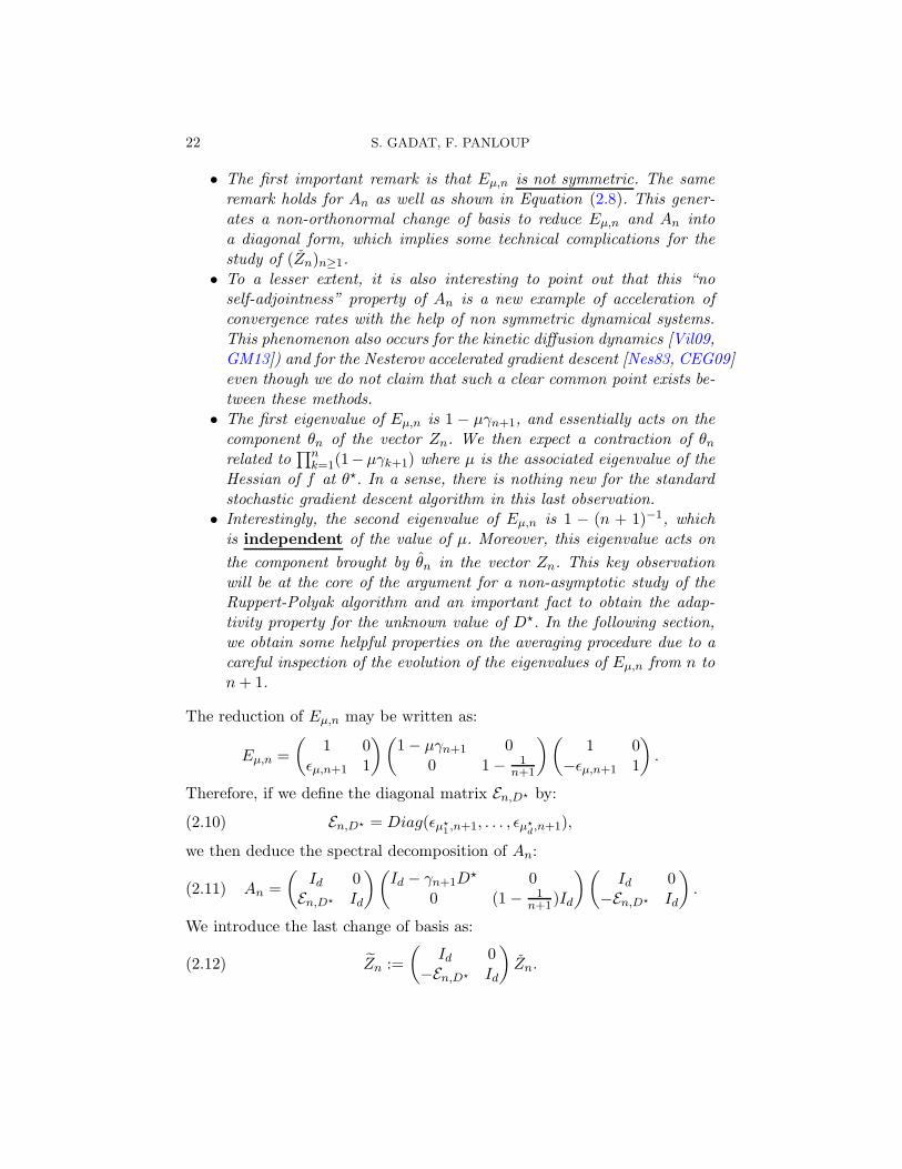
• The first important remark is that Eµ,n is not symmetric. The sameremark holds for An as well as shown in Equation (2.8). This gener-ates a non-orthonormal change of basis to reduce Eµ,n and An intoa diagonal form, which implies some technical complications for thestudy of (Zn)n≥1.

• To a lesser extent, it is also interesting to point out that this “noself-adjointness” property of An is a new example of acceleration ofconvergence rates with the help of non symmetric dynamical systems.This phenomenon also occurs for the kinetic diffusion dynamics [Vil09,GM13]) and for the Nesterov accelerated gradient descent [Nes83, CEG09]even though we do not claim that such a clear common point exists be-tween these methods.

• The first eigenvalue of Eµ,n is 1 − µγn+1, and essentially acts on thecomponent θn of the vector Zn. We then expect a contraction of θnrelated to

∏nk=1(1−µγk+1) where µ is the associated eigenvalue of the

Hessian of f at θ⋆. In a sense, there is nothing new for the standardstochastic gradient descent algorithm in this last observation.

• Interestingly, the second eigenvalue of Eµ,n is 1 − (n + 1)−1, whichis independent of the value of µ. Moreover, this eigenvalue acts on

the component brought by θn in the vector Zn. This key observationwill be at the core of the argument for a non-asymptotic study of theRuppert-Polyak algorithm and an important fact to obtain the adap-tivity property for the unknown value of D⋆. In the following section,we obtain some helpful properties on the averaging procedure due to acareful inspection of the evolution of the eigenvalues of Eµ,n from n ton+ 1.

The reduction of Eµ,n may be written as:

Eµ,n =

(1 0

ǫµ,n+1 1

)(1 − µγn+1 0

0 1 − 1n+1

)(1 0

−ǫµ,n+1 1

).

Therefore, if we define the diagonal matrix En,D⋆ by:

(2.10) En,D⋆ = Diag(ǫµ⋆1,n+1, . . . , ǫµ⋆

d,n+1),

we then deduce the spectral decomposition of An:

(2.11) An =

(Id 0

En,D⋆ Id

)(Id − γn+1D

⋆ 00 (1 − 1

n+1)Id

)(Id 0

−En,D⋆ Id

).

We introduce the last change of basis as:

(2.12) Zn :=

(Id 0

−En,D⋆ Id

)Zn.


We will establish the following proposition.

Proposition 2.4. Assume that Λ⋆ is a positive-definite matrix. If (θn)n≥1

is a (Lp,√γn)-consistent sequence with p ≥ 4 and if (HS) holds then the

sequence (Zn)n≥0 = (Z(1)n , Z

(2)n )n≥0 satisfies:

• i) Some constants (cp)p≥1 exists such that:

∀n ≥ 1 E

∣∣∣Z(1)n

∣∣∣p. cpγn

p2 .

• ii) A constant c2 exists such that:

∀n ≥ 1 E

∣∣∣Z(2)n

∣∣∣2≤ Tr(Σ⋆)

n+

c2nrβ

,

where rβ = (β + 1/2) ∧ (2 − β) > 1 as soon as β ∈ (1/2, 1).

Since we aim to obtain the highest possible value for the second order termrβ, we are driven to the “optimal” choice β = 3/4, which in turns impliesthat

∀n ∈ N⋆

E|Zn|22 ≤Tr(Σ⋆)

n+ Cn−5/4.

Proof. Proof of i): We first observe that the sequence in Rd × R

d may

be written as Zn = (Z(1)n , Z

(2)n ) and Equations (2.7) and (2.12) prove that

Z(1)n = Qθn. Then, the (Lp,

√γn)-consistency of (Z

(1)n )n≥1 is a direct conse-

quence of the one of (θn)n≥1.

Proof of ii): We pick n0 such that ∀n ≥ n0 : ǫµ,n < 0 for any µ ∈ Sp(Λ⋆).Step 1: Recursion formulaWe first establish a recursion between Zn and Zn+1 that will be used inLemma A.2. It will provide a key relationship on the covariance between

Z(1)n and Z

(2)n and on the variance of Z

(2)n .

Definitions (2.7), (2.12), the recursive link (2.5) and the definition of υngiven in Equation (2.3) yield:

Zn+1 =

(Id 0

−En+1,D⋆ Id

)Zn+1

=

(Id 0

−En+1,D⋆ Id

)(AnZn + γn+1

(Q∆Mn+1Q∆Mn+1

n+1

)+ υn

)

=

(Id 0

−En+1,D⋆ Id

)(Id 0

En,D⋆ Id

)(Id − γn+1D

⋆ 00 (1 − 1

n+1 )Id

)Zn

+ γn+1

[(Q∆Mn+1

(−En+1,D⋆ + Idn+1 )Q∆Mn+1

)+

(Q(Λ⋆ − Λn)θn

(En+1,D⋆ − Idn+1 )Q(Λ⋆ − Λn)θn

)],


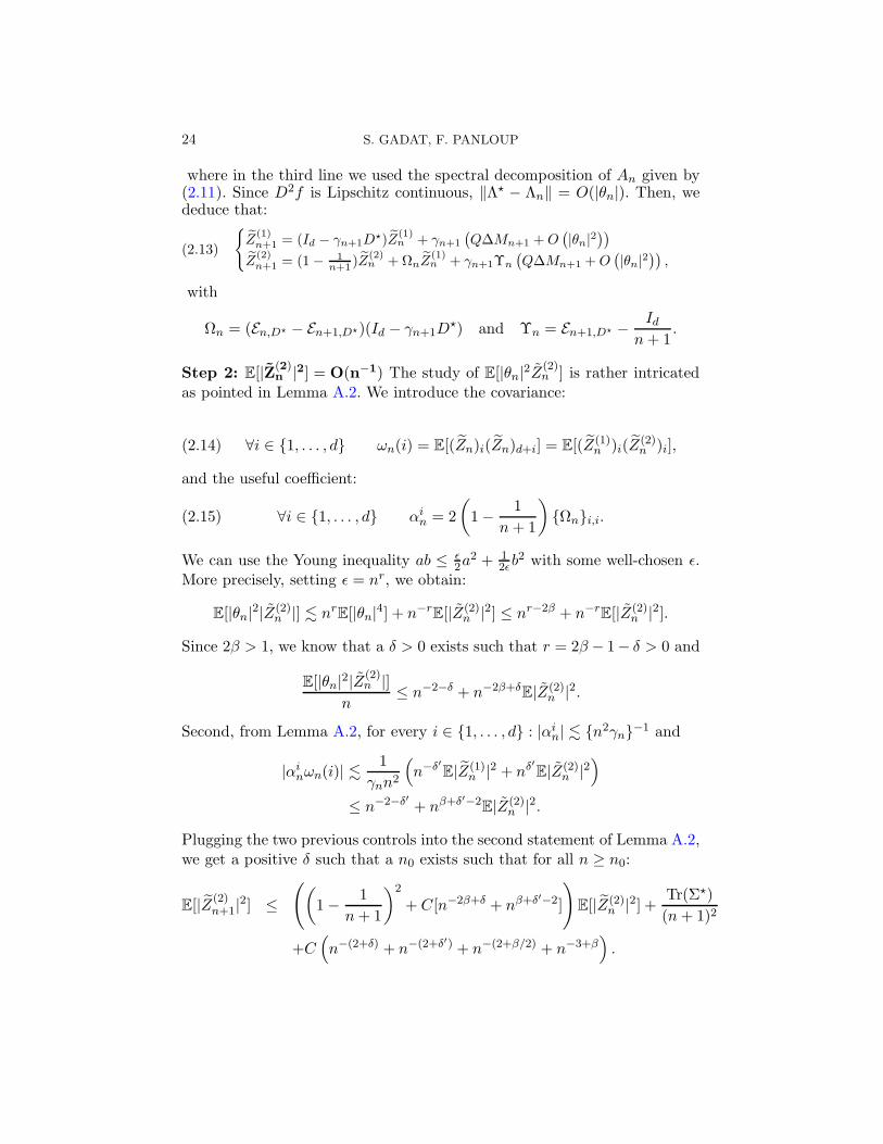
where in the third line we used the spectral decomposition of An given by(2.11). Since D2f is Lipschitz continuous, ‖Λ⋆ − Λn‖ = O(|θn|). Then, wededuce that:

Z

(1)n+1 = (Id − γn+1D

⋆)Z(1)n + γn+1

(Q∆Mn+1 +O

(|θn|2

))

Z(2)n+1 = (1 − 1

n+1 )Z(2)n + ΩnZ

(1)n + γn+1Υn

(Q∆Mn+1 +O

(|θn|2

)),

(2.13)

with

Ωn = (En,D⋆ − En+1,D⋆)(Id − γn+1D⋆) and Υn = En+1,D⋆ − Id

n+ 1.

Step 2: E[|Z(2)n |2] = O(n−1) The study of E[|θn|2Z(2)

n ] is rather intricatedas pointed in Lemma A.2. We introduce the covariance:

(2.14) ∀i ∈ 1, . . . , d ωn(i) = E[(Zn)i(Zn)d+i] = E[(Z(1)n )i(Z

(2)n )i],

and the useful coefficient:

(2.15) ∀i ∈ 1, . . . , d αin = 2

(1 − 1

n+ 1

)Ωni,i.

We can use the Young inequality ab ≤ ǫ2a

2 + 12ǫb

2 with some well-chosen ǫ.More precisely, setting ǫ = nr, we obtain:

E[|θn|2|Z(2)n |] . nrE[|θn|4] + n−r

E[|Z(2)n |2] ≤ nr−2β + n−r

E[|Z(2)n |2].

Since 2β > 1, we know that a δ > 0 exists such that r = 2β − 1− δ > 0 and

E[|θn|2|Z(2)n |]

n≤ n−2−δ + n−2β+δ

E|Z(2)n |2.

Second, from Lemma A.2, for every i ∈ 1, . . . , d : |αin| . n2γn−1 and

|αinωn(i)| . 1

γnn2

(n−δ′

E|Z(1)n |2 + nδ

′

E|Z(2)n |2

)

≤ n−2−δ′ + nβ+δ′−2E|Z(2)

n |2.

Plugging the two previous controls into the second statement of Lemma A.2,we get a positive δ such that a n0 exists such that for all n ≥ n0:

E[|Z(2)n+1|2] ≤

((1 − 1

n+ 1

)2

+ C[n−2β+δ + nβ+δ′−2]

)E[|Z(2)

n |2] +Tr(Σ⋆)

(n+ 1)2

+C(n−(2+δ) + n−(2+δ′) + n−(2+β/2) + n−3+β

).


We choose δ = β − 1/2 > 0 and δ′ = 1/2 − β/2 > 0. In the meantime, wealso have 2 + δ ∧ 2 + δ′ ∧ 2 + β/2 ∧ 3 − β > 2. According to this choice, wecan apply Lemma A.4 and deduce that a η > 0 exists such that:

∀n ≥ 1 E[|Z(2)n+1|2] ≤

Tr(Σ⋆)

n+ 1(1 +O(n−η).

Step 3: Control of the covariance Owing to the previous control of

E[|Z(2)n |2], one can deduce from Cauchy-Schwarz inequality that:

(2.16) E[|θn|2|Z(2)n |] ≤

√E[|θn|4]

√E[|Z(2)

n |2] .γn√n.

Plugging this control into Lemma A.2 i), we obtain that for all i ∈ 1, . . . , d:

ωn+1(i) = (1 − γn+1µ⋆i )

n

n+ 1ωn(i) +O

(γn+1

n+ 1

)+O

(γ2n+1√n

).

Now, remark that γn .√n so that we can conclude that E[|θn|2|Z(2)

n |] shallbe neglected in the evolution of (ωn(i))n≥1:

ωn+1(i) = (1 − γn+1µ⋆i )

n

n+ 1ωn(i) +O

(γn+1

n+ 1

).

From Lemma A.3 stated in Appendix A, we conclude that:

(2.17) ∀i ∈ 1, . . . , d ωn(i) = O

(1

n

).

Step 4: Expansion of the quadratic error We can conclude the proofof Proposition 2.4 ii). From the previous upper bounds (2.17) and (2.16),we have:

d∑

i=1

αinωn(i) = O

(1

n2γn

)×O

(1

n

)and

E[|θn|2|Z(2)n |]

n= O

(γnn√n

).

We use these bounds in the statement of Lemma A.2 ii) and deduce that:

E[|Z(2)n+1|2] ≤

(1 − 1

n+ 1

)2

E[|Z(2)n |2] +O

(1

n3γn

)+O

(γn

n3

2

)+O

(√γn

n2

)

≤(

1 − 1

n+ 1

)2

E[|Z(2)n |2] +O

(1

n(3

2+β)∧(3−β)

)

where we used that γn = γn−β so that√γnn

−2 = o(γnn−3/2) regardless

the value of β ∈ (1/2, 1). Applying again Lemma A.4 with r = +∞ andqβ = (32 + β) ∧ (3 − β), one obtains the announced result.


Remark 2.2 (About the linear case). When x 7→ D2f(x) is constant (oralso when the function f to minimize is C3 with a third partial deriva-tives Lipschitz and null at θ⋆), we can remark that Λn = Λ⋆ (or thatΛn − Λ⋆ = O(|θn|2)). Following carefully the proof of Lemma A.2, we can

deduce that the error term n−1O(E[|θn|2|Z(2)n |]) vanishes (or is replaced by

n−1O(E[|θn|3|Z(2)n |]) . (n−1γn)

3

2 if the (L6,√γn)-consistency holds). Hence:

E[|Z(2)n+1|2] ≤

(1 − 1

n+ 1

)2

E[|Z(2)n |2] +O(n−3γ−1

n ) +O

(√γn

n2

).

The rate is then optimized by choosing β = 2/3, leading to an exponent n−4

3 .

3. (Lp,√

γn)-consistency - (Theorem 3). The main objective of thissection is to prove Theorem 3 iii). Our analysis is based on a Lyapunov-typeapproach with the help of Vp : Rd → R defined for a given p ≥ 1 by:

Vp(x) = fp(x) exp(φ(f(x)).

We have the following result:

Theorem 4 (Convergence rate of (θn)n≥1 with Hφ ). Let p ≥ 1 and assume

(Hφ) and (HφΣp

). Let (γn)n→ be a non-increasing sequence such that γn → 0as n→ +∞. Then,

i) An integer n0 ∈ N and some positive c1 and c2 exist such that

(3.1) ∀n ≥ n0, E[Vp(θn+1)] ≤ (1 − c1γn+1)E[Vp(θn)] + c2γp+1n+1.

ii) Furthermore, if γn − γn+1 = o(γ2n+1) as n→ +∞, then

∀n ≥ 1 E [Vp(θn)] ≤ Cpγnp.In particular,

∀n ≥ 1 E[fp(θn)] ≤ Cpγnp.

Note that the condition γn − γn+1 = o(γ2n+1) is satisfied when γn = γn−β

with β ∈ (0, 1). Therefore, Theorem 3 iii) holds true.To prove Theorem 4 i), we need some technical results related to φ and Vp.The first result is a simple sub-additive property on φ that essentially relieson the concavity property on [x0,+∞).

Lemma 3.1. Assume that φ satisfies (Hφ)(i), then a constant cφ exists suchthat for all x, y ∈ R+:

φ(x + y) ≤ φ(x) + φ(y) + cφ.


Proof. Since φ′′ ≤ 0 on [x0,+∞), the function φ is concave on [x0,+∞).Hence, the function x 7→ φ(x + y) − φ(x) is decreasing on [x0,+∞) and wededuce that:

∀x ≥ x0 φ(x + y) ≤ φ(x) + φ(x0 + y) − φ(x0).

Since φ′ is decreasing on [x0,+∞), then φ′ is upper-bounded and a constantC > 0 exists such that φ(y + x0) ≤ φ(y) + Cx0. We then deduce that:

(3.2) ∀x ≥ x0 ∀y ≥ 0 φ(x + y) ≤ φ(x) + φ(y) + Cx0 − φ(x0).

In the other situation when x ≤ x0, the fact that φ is non-decreasing yieldsand Equation (3.2) applied at point x0 yields:

φ(x + y) ≤ φ(x0 + y) ≤ φ(y) + Cx0 ≤ φ(x) + φ(y) + Cx0.

We then obtain the desired inequality for any value of x and y in R+.

The second key element of our study is a straightforward computation ofthe first and second derivatives of Vp.

Lemma 3.2. For any p ∈ N⋆ and any x ∈ R

d \ θ⋆, we have:

i)

∇Vp(x) = Vp(x)

(p∇f(x)

f(x)+ φ′(f(x))∇f(x)

).

ii)D2Vp(x) = Vp(x)

[ψ1(x)∇f(x) ⊗∇f(x) + ψ2(x)D2f(x)

],

where ψ1 and ψ2 are given by:

ψ1(x) :=

(p

f(x)+ φ′(f(x))

)2

− p

f2(x)+φ′′(f(x)) and ψ2(x) :=

p

f(x)+φ′(f(x)).

Lemma 3.3. Assume that f satisfies (Hφ), then one has

i) A constant α > 0 exists such that:

infx∈Rd

〈∇Vp(x),∇f(x)〉Vp(x)

≥ α > 0.

ii) For any matrix norm ‖ . ‖, a positive constant C > 0 exists such thatfor any ξ ∈ R

d,

‖D2Vp(ξ)‖ ≤ C

(Vp−1(ξ) +

Vp(ξ)

1 + |∇f(ξ)|2).


Proof. Below, C refers to a large enough constant independent of ξ whosevalue may change from line to line.i) We apply Lemma 3.2 i) and obtain that:

∀x ∈ Rd \ θ⋆ 〈∇Vp(x),∇f(x)〉

Vp(x)= p

‖∇f(x)‖2f(x)

+ φ′(f(x))‖∇f(x)‖2.

The result then follows from Assumption (Hφ)ii) and a continuity argumentaround θ⋆.ii) We apply Lemma 3.2 ii) and write that ∀y ∈ R

d:

〈y,D2Vp(ξ)y〉‖y‖2 = Vp(ξ)

[ψ1(ξ)〈y,∇f(ξ) ⊗∇f(ξ)y〉 + ψ2(ξ)〈y,D2f(ξ)y〉

]

≤ Vp(ξ)

([2p2

f2(ξ)+ 2φ′(f(ξ))2 − p

f2(ξ)+ φ′′(f(ξ))

]‖∇f(ξ)‖2

+

[p

f(ξ)+ φ′(f(ξ))

]‖D2f(ξ)‖

).

We now apply assumption Hφ: a large enough constant C exists such that:

‖∇f(ξ)‖2f2(ξ)

≤ C

f(ξ)and φ′(f(ξ))2‖∇f(ξ)‖2 ≤ Cφ′(f(ξ)).

Since ξ 7−→ ‖D2f(ξ)‖ is bounded under Assumption Hφ from the normequivalence in any finite dimensional real vector space, we then have that:

〈y,D2Vp(ξ)y〉‖y‖2 ≤ CVp(ξ)

[1

f(ξ)+ φ′(f(ξ)) + φ′′(f(ξ))

]

≤ CVp−1(ξ) +CVp(ξ)

1 + ‖∇f(ξ)‖2(1 + ‖∇f(ξ)‖2

)(φ′(f(ξ)) + φ′′(f(ξ))) .

Since φ′′(u) is negative for u large enough, that φ′ is bounded (it is anon-increasing function on [x0,+∞)) and that Assumption Hφ implies thatlim φ′(f(ξ))|∇f(ξ)|2 < +∞, we then deduce that:

supξ∈Rd

(φ′(f(ξ)) + φ′′(f(ξ))(1 + |∇f(ξ)|2) < +∞.

Hence,

∀y ∈ Rd 〈y,D2Vp(ξ)y〉

‖y‖2 ≤ C

(Vp−1(ξ) +

Vp(ξ)

1 + ‖∇f(ξ)‖2).

The second assertion follows.

The next lemma will be useful to produce an efficient descent inequality.


Lemma 3.4. Suppose that Hφ holds and consider ρ ∈ [0, 1]. For any γ > 0,ε > 0 define ξγ,ε,x = x+ ργ (−∇f(x) + ε). Then,

i) A γ0 > 0, a constant C > 0 independent of ρ and ε > 0 exist such thatfor any γ ∈ [0, γ0] such that:

f(ξγ,ε,x) ≤ f(x) + Cγ|ε|2.

ii) If 2γ‖D2f‖∞ ≤ 1, then ∀ρ > 0 : ∃ cρ > 0 : ∀x ∈ Rd :

γ2D2Vp(ξγ,ε,x) (−∇f(x) + ε)⊗2

≤ C(1 + |ε|2(p+1)) exp(φ(γ|ε|2))(ργVp(x) + γ2Vp(x) + (cρ + 1)γp+1

).

Proof. C is a positive constant whose value may change from line to line.i) Using the Taylor formula, a ξ exists on the segment [x, ξγ,ε,x] such that:

f(ξγ,ε,x) = f(x)−ργ‖∇f(x)‖2+ργ〈∇f(x), ε〉+ρ2γ2

2D2f(ξ) (−∇f(x) + ε)⊗2 .

Hφ implies that D2f is upper bounded and ‖a+b‖2 ≤ 2(‖a‖2 +‖b‖2) yields:

D2f(ξ) ((−∇f(x) + ε)⊗2 ≤ 2‖D2f‖∞(‖∇f(x)‖2 + ‖ε‖2

).

By the elementary inequality |〈u, v〉| ≤ 12 (‖u‖2 + ‖v‖2) we deduce that:

f(ξγ,ε,x) ≤ f(x) − ργ‖∇f(x)‖2 + ργ〈∇f(x), ε〉 + Cρ2γ2

2

(‖∇f(x)‖2 + ‖ε‖2

)

≤ f(x) + ργ

[−1

2+ ργ‖D2f‖∞

]‖∇f(x)‖2 +

[ργ2

+ ‖D2f‖∞ρ2γ2]‖ε‖2

≤ f(x) + ργ‖ε‖2 ≤ f(x) + γ‖ε‖2,

where in the last line we use that ρ ≤ 1 and the condition γ‖D2f‖∞ ≤ 1/2.The result follows by choosing γ0 ≤ C−1.

ii) We divide the proof into 4 steps.• Step 1: Comparison between Vr(ξγ,ε,x) and Vr(x). Let r ≥ 0. Since φ is

non-decreasing, one first deduces from i) that a constant C > 0 exists suchthat:

Vr(ξγ,ε,x) ≤ (f(x) + Cγ‖ε‖2)r exp(φ(f(x) + γ‖ε‖2)

).

The sub-additivity property of Lemma 3.1 associated with (|a| + |b|)r ≤2r(|a|r + |b|r) yields:

Vr(ξγ,ε,x) ≤ 2r(f r(x) + (Cγ)r‖ε‖2r

)eφ(f(x))+φ(γ‖ε‖2)+cφ .


Setting Tε,γ,r = (1 + ‖ε‖2r) exp(φ(γ‖ε‖2), and using that V0 = eφ(f):

∀r ≥ 0 ∃Cr > 0 Vr(ξγ,ε,x) ≤ Cr exp(φ(γ‖ε‖2)[Vr(x) + γr‖ε‖2rV0(x)

]

≤ Cr exp(φ(γ‖ε‖2)[(1 + ‖ε‖2r)Vr(x) + γr‖ε‖2r

]

≤ CrTε,γ,r [Vr(x) + γr] .(3.3)

where in the second line, we used that V0 ≤ c(1 + Vr).• Step 2: Upper bound of D2Vp(ξγ,ε,x)‖.‖∇f(x)‖2. We apply Lemma 3.3 ii)

with ξ = ξγ,ε,x and we obtain that:

‖D2Vp(ξγ,ε,x)‖.‖∇f(x)‖2 ≤ C

(Vp−1(ξγ,ε,x) +

Vp(ξγ,ε,x)

1 + ‖∇f(ξγ,ε,x)‖2)‖∇f(x)‖2

.

(Tǫ,γ,p−1[Vp−1(x) + γp−1] +

Tε,γ,p[Vp(x) + γp]

1 + ‖∇f(ξγ,ε,x)‖2)‖∇f(x)‖2

. Tǫ,γ,p−1Vp−1(x)[‖∇f(x)‖2 + γp−1‖∇f(x)‖2]

+Tε,γ,p‖∇f(x)‖2

1 + ‖∇f(ξγ,ε,x)‖2 [Vp(x) + γp].

Under Assumption (Hφ), Vp−1(x)‖∇f(x)‖2 ≤ CVp(x) and γp−1‖∇f(x)‖2 ≤Cγp−1f(x) ≤ Cγp−1(1 + Vp(x)). From the boundedness of γ and the trivialinequality since Tǫ,γ,p−1 ≤ 2Tǫ,γ,p, we then deduce that

‖D2Vp(ξγ,ε,x)‖.‖∇f(x)‖2 . Tǫ,γ,p−1[Vp(x) + γp−1] +Tǫ,γ,p[Vp(x) + γp]‖∇f(x)‖2

1 + ‖∇f(ξγ,ε,x)‖2

. Tǫ,γ,p

[[Vp(x) + γp−1] +

[Vp(x) + γp]‖∇f(x)‖21 + ‖∇f(ξγ,ε,x)‖2

],(3.4)

and we are forced to produce an upper bound of ‖∇f(x)‖21+|∇f(ξγ,ε,x)|2 . According

to the Taylor formula, a ξ′ exists in [x, ξγ,ε,x] such that:

∇f(x) = ∇f(ξγ,ε,x) − ργD2f(ξ′) (−∇f(x) + ε) ,

and the triangle inequality yields:

‖∇f(x)‖ ≤ ‖∇f(ξγ,ε,x)‖ + ‖D2f‖∞γ(‖∇f(x)‖ + ‖ε‖),

so that:

‖∇f(x)‖ ≤ (1 − ‖D2f‖∞γ)−1 (‖∇f(ξγ,ε,x)‖ + ‖ε‖) .

The elementary inequality (u+ v)2 ≤ 2(u2 + v2) leads to:

‖∇f(x)‖2 ≤ 8‖∇f(ξγ,ε,x)‖2 + ‖ε‖2).


As a consequence, for a large enough constant C, we have that:

( ‖∇f(x)‖21 + ‖∇f(ξ)‖2 + |ε|2

)≤ C(1 + ‖ε‖2).

Plugging this inequality in (3.4) yields:

‖D2Vp(ξγ,ε,x)‖.‖∇f(x)‖2 . Tǫ,γ,p(γp−1 + [Vp(x) + γp](1 + ‖ε‖2)

),

and since Tε,γ,p(1 + ‖ε‖2) ≤ 3Tε,γ,p+1, we then conclude that:

(3.5) ‖D2Vp(ξγ,ε,x)‖.‖∇f(x)‖2 . Tǫ,γ,p+1

(γp−1 + Vp(x)

),

• Step 3: Upper bound of D2Vp(ξγ,ε,x)‖.‖ǫ‖2. We focus on the noise part ε.

Using (3.3) and Lemma 3.3 ii) once again, we have that:

(3.6) ‖D2Vp(ξγ,ε,x)‖.‖ε‖2 . Tε,γ,p+1

(Vp−1(x) + Vp(x) + γp−1

).

• Step 4: Upper bound of D2Vp(ξγ,ε,x)‖(−∇f(x) + ε)⊗2. We use Equations

(3.5) and (3.6) and obtain:

γ2D2Vp(ξγ,ε,x)(−∇f(x) + ε)⊗2 ≤ CTε,γ,p+1(γ2Vp−1(x) + γ2Vp(x) + γp+1).

To obtain the result, it is now enough to prove for any ρ > 0, a constant cρexists such that:

γ2Vp−1(x) ≤ ργV p(x) + cργp+1.

To derive this key comparison, we use the Young inequality uv ≤ up

p + vq

q

when 1/p + 1/q = 1. In particular, we choose u = ργp−1

p V p−1(x), v =γ1+1/pρ−1, p = p/(p− 1), q = p and obtain that

γ2Vp−1(x) = exp(φ(γ‖ǫ‖2))γ2fp(x)

≤ exp(φ(γ‖ǫ‖2))

[p− 1

p

(ργ(p−1)/pfp−1(x)

)p/(p−1)+γp+1

pρp

]

≤ p− 1

pρp/(p−1)γVp(x) + p−1ρ−pγp+1 exp(φ(γ‖ǫ‖2))

≤ p− 1

pρp/(p−1)γVp(x) + p−1ρ−pγp+1V0(x)

Using V0 ≤ C(1 + Vp) once again, we then deduce that for any ρ > 0, aconstant cρ exists such that:

γ2Vp−1(x) ≤ ργVp(x) + cργp+1.


We obtain the final upper bound:∀ρ > 0 ,∃ cρ > 0 ,∀x ∈ Rd :

γ2D2Vp(ξγ,ε,x) (−∇f(x) + ε)⊗2 ≤ CTǫ,γ,p+1

(ργVp(x) + γ2Vp(x) + (cρ + 1)γp+1

).

We now focus on the proof of Theorem 4 i).

Proof of Theorem 4. i) We apply the second order Taylor formula toVp and obtain that:

Vp(θn+1) = Vp(θn) − γn+1〈∇Vp(θn),∇f(θn)〉 + γn+1〈Vp(θn),∆Mn+1〉

+γ2n+1

2D2Vp(ξn+1)(−∇f(θn) + ∆Mn+1)

⊗2,

where ξn+1 = θn + ρ∆θn+1, ρ ∈ [0, 1]. Using Lemma 3.3 i), we obtain thata α > 0 exists such that:

(3.7) ∀n ∈ N⋆ Vp(θn) − γn+1〈∇Vp(θn),∇f(θn)〉 ≤ Vp(θn)(1 − αγn+1).

Moreover, we have that E[γn+1〈Vp(θn),∆Mn+1〉 | Fn] = 0. Finally, Lemma3.4 ii) shows that a constant C > 0 exists such that for any ρ > 0 , for alln ∈ N

⋆, cρ exists such that:

γ2n+1

2D2Vp(ξn+1)(−∇f(θn) + ∆Mn+1)

⊗2

≤ CT∆Mn+1,γn+1,p+1

(ργn+1Vp(θn) + γ2n+1Vp(θn) + (cρ + 1)γn+1p+1

).

This last upper bound associated with (3.7) and Assumption (HφΣp

) yields:

E [Vp(θn+1) | Fn]

≤ (1 − αγn+1)Vp(θn) +

C(ργn+1Vp(θn) + γ2n+1Vp(θn) + (cρ + 1)γn+1p+1

)E[T∆Mn+1,γn+1,p+1 | Fn

]

≤ (1 − αγn+1)Vp(θn) + CΣp

(ργn+1Vp(θn) + γ2n+1Vp(θn) + (cρ + 1)γn+1p+1

)

≤ (1 − (α− ρCΣp)γn+1 + CΣpγ2n+1)Vp(θn) + (1 + cρ)CΣpγn+1p+1.

We now choose ρ such that ρCΣp = α2 and determine that two non-negative

constants c1 and c2 exist such that ∀n ∈ N⋆:

(3.8) E [Vp(θn+1) | Fn] ≤(

1 − α

2γn+1 + c1γ

2n+1

)Vp(θn) + c2γn+1p+1.

Theorem 4 i) easily follows by taking the expectation and by using thatc1γn+1 ≤ α/4 for n large enough.


ii) We prove by induction that a large enough C > 0 exists such that:

(3.9) ∀n ∈ N⋆

E [Vp(θn)] ≤ C γnp .

Since γn − γn+1 = o(γ2n+1) as n→ +∞(

γnγn+1

)p

≤ 1 + o(γn+1) as n→ +∞,

a sufficiently large n1 exists such that

(3.10) ∀n ≥ n1 0 ≤ (1 − c1γn+1)

(γnγn+1

)p

≤ 1 − c12γn+1.

We can choose C1 large enough such that Equation (3.9) holds true for anyn ≤ n1 with C ≥ C1. For any n1 ∈ N, the result holds for any n ≤ n1.Assuming that the property holds at a given rank n ≥ n1, we then have:

E[Vp(θn+1)] ≤ (1 − c1γn+1)E[Vp(θn)] + c2γn+1p+1.

≤ (1 − c1γn+1)Cγpn + c2γn+1p+1.

≤ Cγn+1p[(

γnγn+1

)p

(1 − c1γn+1) +c2Cγn+1

]

≤ Cγn+1p[1 −

(c12

− c2C

)γn+1

]

where we used Equation (3.1), the induction property (3.9) and Inequality(3.10). If we choose C ≥ C2 = c2

2c1, then E[Vp(θn)] ≤ Cγpn =⇒ E[Vp(θn+1)] ≤

C γn+1p. This ends the proof of ii).

Acknowledgments. The authors gratefully acknowledge Jerome Bolteand Gersende Fort for stimulating discussions on the Kurdyka- Lojasiewiczinequality and averaged stochastic optimization algorithms.

References.

[ABRW12] A. Agarwal, P. L. Bartlett, P. Ravikumar, and M. J. Wainwright. Information-theoretic lower bounds on the oracle complexity of stochastic convex optimiza-tion. IEEE Transactions on Information Theory, 58(5):3235–3249, May 2012.

[Bac14] F. Bach. Adaptivity of averaged stochastic gradient descent to local strongconvexity for logistic regression. J. Mach. Learn. Res., 15:595–627, 2014.

[BDL06] J. Bolte, A. Daniilidis, and A. Lewis. The lojasiewicz inequality for nonsmoothsubanalytic functions with applications to subgradient dynamical systems.SIAM J. Optim., 17(4):1205–1223, 2006.


[BDLM10] J. Bolte, A. Daniilidis, O. Ley, and L. Mazet. Characterizations of lojasiewiczinequalities: subgradient flows, talweg, convexity. Trans. Amer. Math. Soc.,(362):3319–3363, 2010.

[Ber99] D. P. Bertsekas. Nonlinear programming. Athena Scientific Optimization andComputation Series. Athena Scientific, Belmont, MA, second edition, 1999.

[BM11] F. Bach and E. Moulines. Non-asymptotic analysis of stochastic approxi-mation algorithms for machine learning. Advances in Neural InformationProcessing Systems, 2011.

[BNPS16] J. Bolte, P. Nguyen, J. Peypouquet, and B. W. Suter. From error boundsto the complexity of first-order descent methods for convex functions. Math.Program. (A), to appear, pages 1–37, 2016.

[CB01] G. Casella and R.L. Berger. Statistical Inference. Duxbury Press, 2001.[CCGB17] H. Cardot, P. Cenac, and A. Godichon-Baggioni. Online estimation of the

geometric median in Hilbert spaces: Nonasymptotic confidence balls. Ann.Statist., 45(2):591–614, 2017.

[CCZ13] H. Cardot, P. Cenac, and P.A. Zitt. Efficient and fast estimation of the geomet-ric median in hilbert spaces with an averaged stochastic gradient algorithm.Bernoulli, 19:18–43, 2013.

[CEG09] A. Cabot, H. Engler, and S. Gadat. On the long time behavior of second orderdifferential equations with asymptotically small dissipation. Trans. Amer.Math. Soc., 361(11):5983–6017, (2009).

[Duf97] M. Duflo. Random Iterative Models, Adaptive algorithms and stochastic ap-proximations. Applications of Mathematics. Springer-Verlag, New-York, 1997.

[For15] G. Fort. Central limit theorems for stochastic approximation with controlledMarkov chain dynamics. ESAIM Probab. Stat., 19:60–80, 2015.

[GM13] S. Gadat and L. Miclo. Spectral decompositions and l2-operator norms of toyhypocoercive semi-groups. Kinetic and Related Models, 6:317–372, 2013.

[Kem87] J.H.B. Kemperman. The median of a finite measure on a banach space. Sta-tistical data analysis based on the L1-norm and related methods (Neuchtel,1987), pages 217–230, 1987.

[Kur98] K. Kurdyka. On gradients of functions definable in o-minimal structures. Ann.Inst. Fourier (Grenoble), 48(3):769–783, 1998.

[Loj63] S. Lojasiewicz. Une propriete topologique des sous-ensembles analytiquesreels. Editions du centre National de la Recherche Scientifique, Paris, LesEquations aux Derivees Partielles, pages 87–89, 1963.

[Nes83] Y. Nesterov. A method of solving a convex programming problem with con-vergence rate o(1/k2). Soviet Mathematics Doklady, 27(2):372–376, 1983.

[Nes04] Y. Nesterov. Introductory Lectures on Convex Optimization. A basic course.Applied Optimization. Kluwer Academic Publishers, Boston, MA, 2004.

[NY83] A. Nemirovski and D. Yudin. Problem complexity and method efficiency inoptimization. Wiley-Interscience Series in Discrete Mathematics., John Wiley,XV, 1983.

[PJ92] B. T. Polyak and A. Juditsky. Acceleration of stochastic approximation byaveraging. SIAM Journal on Control and Optimization, 30:838–855, 1992.

[RM51] H. Robbins and S. Monro. A stochastic approximation method. Ann. Math.Statist., 22:400–407, 1951.

[Rup88] D. Ruppert. Efficient estimations from a slowly convergent robbins-monroprocess. Technical Report, 781, Cornell University Operations Research andIndustrial Engineering, 1988.

[Vil09] C. Villani. Hypocoercivity. Mem. Amer. Math. Soc., 202(950), 2009.


APPENDIX A: TECHNICAL LEMMAS FOR THEOREM 2

The next lemma is important to obtain the stability of the change of basisfrom one iteration to another in our spectral analysis of (θn)n≥1.

Lemma A.1. Assume that γn = γn−β with β ∈ (0, 1). Let µ > 0. Then, aconstant C and an integer n0 exist such that

∀n ≥ n0, |ǫµ,n − ǫµ,n+1| ≤ Cnβ−2

Proof. We choose n0 such that 1 − µγnn < 0 for all n ≥ n0. Then, thedesired inequality comes from a direct computation:

ǫµ,n − ǫµ,n+1 =1 − µγn

1 − µγnn− 1 − µγn+1

1 − µγn+1(n+ 1)

=(1 − µγn)(1 − µγn+1(n+ 1)) − (1 − µγn+1)(1 − µγnn)

(1 − µγnn)(1 − µγn+1(n+ 1))

= µ(γn+1 − γn) + (nγn − (n+ 1)γn+1) + µγnγn+1

(1 − µγnn)(1 − µγn+1(n + 1))

Now, if C denotes a constant that only depends on µ and β (whose valuemay change from line to line), we then have the following inequalities:

|γn+1−γn| ≤ Cn−(1+β), |nγn − (n + 1)γn+1| ≤ Cn−β and γnγn+1 ≤ Cn−2β.

Since β < 1, the denominator is equivalent to n2−2β and we obtain that

(A.1) |ǫµ,n − ǫµ,n+1| ≤ Cn−β

n2−2β= Cnβ−2,

which ends the proof.

Lemma A.2. Under the assumptions of Proposition 2.4, we have:

i) For any i ∈ 1, . . . , d, ωn(i) = E[(Z(1)n )i(Z

(2)n )i] satisfies ∀n ≥ n0,

ωn+1(i) = (1 − γn+1µ⋆i )

n

n+ 1ωn(i) +O

(γn+1

n+ 1

)+O(γn+1E[|θn|2|Z(2)

n |]).

ii) The following recursion holds for any n ≥ n0,

E[|Z(2)n+1|2] =

(1 − 1

n+ 1

)2

E[|Z(2)n |2] +

d∑

i=1

αinωn(i) +

E[|θn|2|Z(2)n |]

n

+Tr(Σ⋆)

(n+ 1)2+O

(√γn

n2∨ 1

n3γn

),

where αin is defined in (2.15) and satisfies |αi

n| . γ−1n n−2, i = 1, . . . , d.


Proof. Set µ = minµ⋆i , i = 1, . . . , d > 0. Recall that n0 ∈ N is such that1 − µγnn < 0 for all n ≥ n0. For all n ≥ n0, Υn and Ωn are well-defineddeterministic matrices and since for a given µ > 0, ǫµ,n ∼ (nγn)−1 andǫµ,n − ǫµ,n+1 = O(n−2γ−1

n ) (see (A.1)), we have

(A.2) γn+1‖Υn‖ = O

(1

n

)and γn+1‖Ωn‖ = O

(1

n2

).

Now, let us prove the first statement.

i) Using (2.13), we have

ωn+1(i) = (1 − γn+1µ⋆i )

(1 − 1

n+ 1

)ωn(i) +O(γn+1E[|θn|2|Z(2)

n |])

+ γ2n+1E[Q∆Mn+1iΥnQ∆Mn+1i] +O(γn+1r(1)n )

where

r(1)n = ‖Ωn‖(E|Z(1)

n |2γn+1

+ E[|θn|2|Z(1)n |]

)+‖Υn‖

(E[|Z(1)

n |.|θn|2] + γn+1E|θn|4).

The Cauchy-Schwarz inequality, the fact that |Z(1)n | = |θn| and the consis-

tency condition lead to

E[|θn|2|Z(1)n |] ≤

E[|θn|4|

1/2 E[|Z(1)

n |2]1/2

≤ γ3/2n+1.

Therefore, (A.2) yields:

γn+1r(1)n .

1

n2

(1 + γ

3

2

n+1

)+

1

n

(γ

3

2

n+1 + γ3n+1

)= o

(γnn

).

In the meantime, under (HS) and because Q ∈ Od(R), we have:

∀i ∈ 1, . . . , d |E[Q∆Mn+1i ΥnQ∆Mn+1i]| . ‖Υn‖E[|∆Mn+1|2]

. ‖Υn‖E‖S(θn)‖

. ‖Υn‖(1 + E|θn|)

. ‖Υn‖.

We therefore deduce from (A.2) and from the previous lines that

∀i ∈ 1, . . . , d γ2n+1 |E[Q∆Mn+1i ΥnQ∆Mn+1i]| .γnn.


ii) We define ∆Nn+1 = ΥnQ∆Mn+1 and recall that αin is defined in (2.15)

by αin = 2(1 − (n + 1)−1)(Ωn)i,i. Starting from (2.13) and |Z(1)

n | = |θn|, weuse that Ωn is a diagonal matrix so that

E[|Z(2)n+1|2] =

(1 − 1

n+ 1

)2

E[|Z(2)n |2] +

d∑

i=1

αinωn(i) + γ2n+1E|∆Nn+1|2

+O(γn+1‖Υn‖E[|θn|2|Z(2)

n |])

+O(γn+1r(2)n ),

where r(2)n is defined by

r(2)n =‖Ωn‖2E|θn|2

γn+1+ ‖Ωn‖‖Υn‖E|θn|3 + γn+1‖Υn‖2E|θn|4.

The (L4,√γn)-consistency, the Jensen inequality and (A.2) yield

γn+1r(2)n = O

(1

γnn4+

√γn

n3+γ2nn2

)= O

(1

n3

)

since γn ≤ cn−1

2 . To achieve the proof, it remains to show that

(A.3) E|∆Nn+1|2 =Tr(Σ⋆)

n2+O

(√γn

n2∨ 1

n3γn

)

First, set Bn = QTΥ2nQ. Using that Υn is a diagonal matrix, we have

|∆Nn+1|2 = Tr(|∆Nn+1|2) = Tr(∆NTn+1∆Nn+1)

= Tr(∆MTn+1Bn∆Mn+1)

= Tr(Bn∆Mn+1∆MTn+1)

Since the trace is a linear application and Bn is a deterministic matrix,

(A.4) E[|∆Nn+1|2|Fn] = Tr(BnE[∆Mn+1∆MTn+1|Fn]) = Tr(BnS(θn))

where we applied Assumption (HS). We also have S(θn) = S(θ⋆) +O(|θn|).For Bn, we first remark that

γn+1Υn = (n+ 1)−1D⋆−1 + ∆n+1

where (∆n)n≥0 is a sequence of matrices defined by:

∆n = Diag

1 − (n+ 1)µ⋆i 2γ2n+1

(n+ 1)µ⋆i ((n + 1)γn+1µ⋆i − 1)+γn+1

n+ 1, i = 1, . . . , d

.


Using that nγ2n → 0 as n→ +∞, one easily checks that

‖∆n‖ .1

n2γn+γnn

.1

n2γn.

As a consequence,

γ2n+1Bn = QT γn+1Υn2Q= QT (n + 1)−1D⋆ + ∆n+12Q

= (n+ 1)−2QT D⋆−2Q+O

(1

n3γn

).

It follows from (A.4) that

γ2n+1E[|∆Nn+1|2|Fn] = γ2n+1Tr(Bn∆Mn+1∆MTn+1)

=Tr(Λ⋆−2S(θ⋆))

(n+ 1)2+O

(E|θn|n2

∨ 1

n3γn

)

=Tr(Λ⋆−2S(θ⋆))

(n+ 1)2+O

(√γn

n2∨ 1

n3γn

)

because which leads to (A.3) and achieves the proof.

Lemma A.3. Assume that (un)n≥0 is a sequence which satisfies for alln ≥ n0 and for a given µ > 0:

un+1 = (1 − γn+1µ)n

n+ 1un + βn+1

with βn . γnn−1. Then, un = O(n−1).

Proof. With the convention∏

∅ = 1 and∑

∅ = 0, we have for every n ≥ n0:

un =

n∏

k=n0+1

(1 − γkµ)k

k + 1

un0

+

n∑

k=n0+1

βk

n∏

ℓ=k+1

(1 − γℓµ)ℓ

ℓ+ 1.

Using that for any x > −1, log(1 + x) ≤ x, we obtain for every n ≥ n0 + 1

n∏

k=n0+1

(1 − γkµ)k

k + 1≤ n0n+ 1

e−µ(Γn−Γn0) ≤ Cn0

e−Γn

n+ 1= O(n−1)

and,

n∑

k=n0+1

βk

n∏

ℓ=k+1

(1 − γℓµ)ℓ

ℓ+ 1≤ 1

n+ 1

e−µΓn

n∑

k=n0+1

βk(k + 1)eµΓk

.


But βk(k + 1) . γk+1. Thus, since x 7→ xeµx is increasing on R+,

n∑

k=n0+1

βk(k + 1)eµΓk .

n∑

k=n0+1

γk+1eµΓk ≤

∫ Γn+1

Γn0+1

eµxdx

and hence,

1

n+ 1

e−µΓn

n∑

k=n0+1

βk(k + 1)eµΓk

≤ Cn0

n+ 1.

The result follows.

Remark A.1. By the expansion log(1+x) = x+c(x)x2 where c is boundedon [−1/2, 1/2], a slight modification of the proof leads to lim infn→+∞ nun >0 when

∑γ2k < +∞.

Lemma A.4. For any sequence (un)n≥0 that satisfies

∀n ≥ 0 un+1 ≤ un

(1 − 1

n+ 1

)2

(1 + 2n−r) +V

(n+ 1)2+ cn−q,

with r ≥ 1 and q ≥ 2, then a large enough constant C independent of nexists such that

∀n ≥ 1 un ≤ V

n+ Cn−r∧(q−1).

Proof. We establish the result using an induction and denote by α = r∧ qThe statement of the lemma is obvious for n = 1 by choosing a large enoughC. Assuming now that the result holds for the integer n, we write

un+1 ≤(

n

n+ 1

)2

(1 + 2n−r)

[V

n+ Cn−α

]+

V

(n+ 1)2+ cn−q

≤ V

[n

(n+ 1)2+

1

(n + 1)2

]+ 2V

(n

n+ 1

)2

n−(r+1)

+Cn−α

(n

n+ 1

)2

+ 2Cn−(α+r)

(n

n+ 1

)2

+ cn−q

=V

n+ 1+ C(n+ 1)−αAn

where

An :=2V n1−r(n+ 1)α−2

C+

(n

n+ 1

)2−α

+ 2n2−α−r

(n + 1)2−α+c

Cn−q(n+ 1)α


We now choose α < 2 and use the first order approximations:

An = 1 − (2 − α)n−1 + C−1[2V nα−(1+r) + 2n−r + cnα−q

]+ o(n−1).

Then, a large enough C exists such that An ≤ 1 for any n ≥ 1 as soon asthe powers of n are lower than 1 inside the brackets on the right hand sideof the equality above. Hence, α should be chosen such that (1 + r) − α ∧r ∧ α − q ≥ 1 and the largest possible value of α corresponds to thechoice

α = (q − 1) ∧ r.For such a choice, a large enough C exists such that the recursion holds,which ends the proof of Lemma A.4.

APPENDIX B: GROWTH AT INFINITY UNDER THE KL GRADIENTINEQUALITY

In this section, we prove the property (1.7) of Proposition 1.2. Without lossof generality, we can assume that θ⋆ = f(θ⋆) = 0.

Proof. Consider 0 ≤ t ≤ s and x ∈ Rd. We then associate the solution of

the differential equation associated to the flow −∇f initialized at x:

χx(0) = x and χx = −∇f(χx).

The length of the curve L(χx, t, s) is defined by

L(χx, t, s) =

∫ s

t‖χx(τ)‖dτ.

Under Assumption (Hr

KL), we can consider ϕ(a) = a1−r

1−r and we have that

ϕ′(f(x))‖∇f(x)‖ ≥ m > 0.

We now observe that e : s 7−→ ϕ(f(χx(s))) satisfies:

e′(τ) = ϕ′(f(χx(τ)))〈∇f(χx(τ)), χx(τ)〉= −ϕ′(f(χx(τ)))‖∇f(χx(τ))‖2≤ −m‖χx(τ)‖

We deduce that:

(B.1) e(t) − e(s) =

∫ t

se′(τ)dτ ≥ m

∫ s

t‖χx(τ)‖dτ ≥ mL(χx, t, s)


Now choosing t = 0 and s −→ +∞, we have e(0) − lims−→+∞ e(s) =ϕ(f(x)) − ϕ(min f) = ϕ(f(x)), and Equation (B.1) yields

ϕ(f(x)) ≥ mL(χx, 0,+∞) ≥ m‖x‖

because χx(+∞) = arg min f = 0. We deduce that

f(x) ≥ ϕ−1(m‖x‖) = m(1 − r) 1

1−r ‖x‖ 1

1−r .

which is the desired conclusion.

Toulouse School of Economics

Universite Toulouse 1 - Capitole.

21 allees de Brienne

31000 Toulouse, France.

E-mail: [email protected]

Laboratoire Angevin de Recherche en Mathematiques,

Universite d’Angers

2 Boulevard Lavoisier

49045 Angers cedex 01, France.

E-mail: [email protected]

mailto:[email protected]

mailto:[email protected]

Documents

arxiv.org · 2017-09-12 · 2 S. GADAT, F. PANLOUP stochastic algorithm (θn)n≥0 deﬁned by: θ0 ∈ Rd and (1.1) ∀n≥ 0, θn+1 = θn −γn+1Λ(θn,Zn+1), where (γn)n≥1