Embed Size (px)
Citation preview
1
Asociación Argentina de Economía Agraria
ECONOMETRIC ESTIMATION OF FOOD DEMAND
ELASTICITIES FROM HOUSEHOLD SURVEYS IN
ARGENTINA, BOLIVIA AND PARAGUAY
Octubre, 2007
Daniel Lema*
Víctor Brescia*
Miriam Berges**
Karina Casellas**
*Instituto de Economía y Sociología, INTA ** Universidad Nacional de Mar del Plata
2
ECONOMETRIC ESTIMATION OF FOOD DEMAND
ELASTICITIES FROM HOUSEHOLD SURVEYS IN
ARGENTINA, BOLIVIA AND PARAGUAY
Abstract This paper presents an econometric estimation of food demand elasticities for Argentina, Bolivia and Paraguay using household survey data. The empirical approach consists in the estimation of a censored corrected LinQuad incomplete demand system of eleven equations using microdata from national household surveys. The limited dependent variable problem is accounted for using the Shonkwiler and Yen two step estimation procedure. Comparative results suggest distinct consumption behaviors in Argentina, Bolivia and Paraguay. Food demand is in general less elastic in Argentina, particularly for dairy products, beef, chicken wheat and sugar. Estimated magnitudes of income elasticities shows a more elastic response in Argentina for dairy products, beef, chicken and oil. JEL Classification: D12, Q11 Clasificación Temática AAEA: 2.1. Análisis de oferta y demanda; 7.1. Modelos econométricos Key Words: Food Demand, Incomplete demand systems, Household surveys.
Resumen
Este trabajo presenta una estimación de sistemas incompletos de demanda utilizando datos de encuestas de hogares para Argentina, Bolivia y Paraguay. El enfoque empírico consiste en la estimación de un sistema con especificación LinQuad corregido por sesgo de selección y (en el caso de Argentina) precios ajustados por calidad. El problema de la variable dependiente limitada por la numerosa aparición de ceros en casos de no consumo del alimento se trató utilizando la metodología en dos etapas de Shonkwiler y Yen y el problema de ajuste de calidad siguiendo a Cox y Wohlgenant. Los resultados comparativos sugieren que existen distintos patrones de consumo de alimentos entre los países, no sólo determinados por factores culturales o hábitos de consumo. La demanda de alimentos es tiene una menor elasticidad en Argentina, particularmente para productos lácteos, carne vacuna, pollo, trigo y azúcar. Las estimaciones de elasticidades ingreso muestran una respuesta más elástica en Argentina para productos lácteos, carne vacuna, pollo y aceites. JEL Classification: D12, Q11 Clasificación Temática AAEA: 2.1. Análisis de oferta y demanda; 7.1. Modelos econométricos Palabras Clave: Demanda de Alimentos, Sistemas incompletos de demanda, Encuestas a hogares.
1
ECONOMETRIC ESTIMATION OF FOOD DEMAND ELASTICITIES FROM HOUSEHOLD SURVEYS IN ARGENTINA, PARAGUAY AND BOLIVI A
I. Introduction In the literature on demand estimation several theoretical and empirical approaches could be identified: single equation, system equations, time series, cross-section and panel data. Recently, new econometric techniques and the increasing use of cross-section household survey data in applied demand analysis present new opportunities for examination of consumption behavior using demand system approach. One important methodological issue is the many zero observations common in household survey data. The bias in the parameter estimates resulting from the use of only positive consumption values when there are many zero observations is a common result. Several approaches have been used for dealing with the zero values. Usually, some variant of Heckman´s two step technique (Heckman, 1979) is used to solve this censored response problem. Heien and Wessells (1990) present a generalization of this procedure to account for zero expenditure in demand systems. One frequent used methodological approach is the estimation of complete demand systems for food consumption. One of the widely used functional forms derived from constrained utility maximization is the Linear Expenditure System (LES). Several reasons are usually invoked to make use of the LES: 1) it has a straightforward and reasonable interpretation, 2) it is one of the few systems that automatically satisfy all the demand theoretical restrictions and 3) it can be derived from a specific utility function: the Stone-Geary function.1 This kind of system does not allow for inferior goods and all of them behave as gross complementary goods. The estimation of the LES is difficult due to nonlinearity in the coefficients β andγ, which enter the formula in a multiplicative form. Some iterative approaches have been developed to overcome this difficulty (Two-Stage Procedure and Full Information Maximum Likelihood Technique) We follow a different approach, choosing a theoretically consistent demand system with the least theoretical restrictions imposed on the parameter space. We estimate a LinQuad incomplete demand system derived from a “quasi expenditure” function, following Fabiosa and Jensen (2003) who mention several advantages of LinQuad over other complete systems in a censored regression. The availability of detailed household survey data on expenditures and consumption of a wide range of food products for Argentina, Bolivia and Paraguay allows the estimation of incomplete demand system parameters. Our main goal is to estimate a price and income elasticities matrix with a common methodology for economic analysis and comparative purposes. This paper presents the methodology, data sources and estimation results of food demand elasticities for these three countries. The organization of the paper is the following: Section II briefly reviews the theoretical and empirical approach behind this study of applied food demand. Section III describes the dataset for each of the countries, which draws mainly
1 This function assumes a Cobb-Douglas function with an origin P –the subsistence quantities- with linear Engel curves. U = (x1 -γ1)
α (x2 -γ2)β ; α + β = 1. Separability is assumed and it is more plausible when we use broad
groups of goods. Their marginal utilities are independent of the quantities of any other good. There are no cross substitution effects. *Instituto de Economía y Sociología - INTA ** Facultad de Ciencias Económicas y Sociales - Universidad Nacional de Mar del Plata
2
on national surveys on household consumption. Section III presents the econometric estimations and results. Section IV has the final remarks and questions for further research.
II. Demand System Analysis of Food Consumption
Theoretical Background
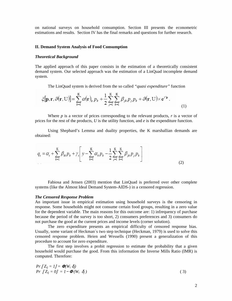
The applied approach of this paper consists in the estimation of a theoretically consistent demand system. Our selected approach was the estimation of a LinQuad incomplete demand system. The LinQuad system is derived from the so called “quasi expenditure” function
(1) Where p is a vector of prices corresponding to the relevant products, r is a vector of prices for the rest of the products, U is the utility function, and e is the expenditure function. Using Shephard’s Lemma and duality properties, the K marshallian demands are obtained:
(2) Fabiosa and Jensen (2003) mention that LinQuad is preferred over other complete systems (like the Almost Ideal Demand System-AIDS-) in a censored regression. The Censored Response Problem An important issue in empirical estimation using household surveys is the censoring in response. Some households might not consume certain food groups, resulting in a zero value for the dependent variable. The main reasons for this outcome are: 1) infrequency of purchase because the period of the survey is too short, 2) consumers preferences and 3) consumers do not purchase the good at the current prices and income levels (corner solution).
The zero expenditure presents an empirical difficulty of censored response bias. Usually, some variant of Heckman´s two step technique (Heckman, 1979) is used to solve this censored response problem. Heien and Wessells (1990) present a generalization of this procedure to account for zero expenditure.
The first step involves a probit regression to estimate the probability that a given household would purchase the good. From this information the Inverse Mills Ratio (IMR) is computed. Therefore:
Pr [ Zij = 1] = ΦΦΦΦ(Wi δj) Pr [ Zij = 0] = 1− ΦΦΦΦ (Wi δj ) ( 3)
3
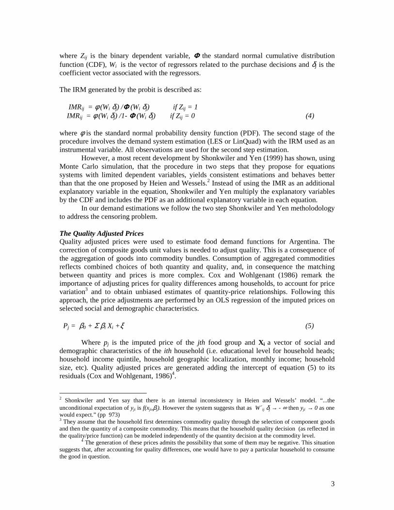
where Zij is the binary dependent variable, ΦΦΦΦ the standard normal cumulative distribution function (CDF), Wi is the vector of regressors related to the purchase decisions and δj is the coefficient vector associated with the regressors. The IRM generated by the probit is described as: IMRij = φ (Wi δj) /ΦΦΦΦ (Wi δj) if Zij = 1 IMRij = φ (Wi δj) /1- ΦΦΦΦ (Wi δj) if Zij = 0 (4) where φ is the standard normal probability density function (PDF). The second stage of the procedure involves the demand system estimation (LES or LinQuad) with the IRM used as an instrumental variable. All observations are used for the second step estimation.
However, a most recent development by Shonkwiler and Yen (1999) has shown, using Monte Carlo simulation, that the procedure in two steps that they propose for equations systems with limited dependent variables, yields consistent estimations and behaves better than that the one proposed by Heien and Wessels.2 Instead of using the IMR as an additional explanatory variable in the equation, Shonkwiler and Yen multiply the explanatory variables by the CDF and includes the PDF as an additional explanatory variable in each equation.
In our demand estimations we follow the two step Shonkwiler and Yen metholodology to address the censoring problem.
The Quality Adjusted Prices Quality adjusted prices were used to estimate food demand functions for Argentina. The correction of composite goods unit values is needed to adjust quality. This is a consequence of the aggregation of goods into commodity bundles. Consumption of aggregated commodities reflects combined choices of both quantity and quality, and, in consequence the matching between quantity and prices is more complex. Cox and Wohlgenant (1986) remark the importance of adjusting prices for quality differences among households, to account for price variation3 and to obtain unbiased estimates of quantity-price relationships. Following this approach, the price adjustments are performed by an OLS regression of the imputed prices on selected social and demographic characteristics. Pj = β0 + Σ βi Xi +ξ (5)
Where pj is the imputed price of the jth food group and Xi a vector of social and demographic characteristics of the ith household (i.e. educational level for household heads; household income quintile, household geographic localization, monthly income; household size, etc). Quality adjusted prices are generated adding the intercept of equation (5) to its residuals (Cox and Wohlgenant, 1986)4.
2 Shonkwiler and Yen say that there is an internal inconsistency in Heien and Wessels’ model. “...the unconditional expectation of yji is f(xji,βj). However the system suggests that as W ij δj → - ∞ then yji → 0 as one would expect.” (pp 973) 3 They assume that the household first determines commodity quality through the selection of component goods and then the quantity of a composite commodity. This means that the household quality decision (as reflected in the quality/price function) can be modeled independently of the quantity decision at the commodity level.
4 The generation of these prices admits the possibility that some of them may be negative. This situation suggests that, after accounting for quality differences, one would have to pay a particular household to consume the good in question.
4
Quality adjusted prices were used for Argentina estimations following the approach presented in Berges and Casellas (2002). The adjustments were made to prices by regressing the imputed prices on selected social and demographic characteristics. The estimated price equations are: Pj = β0 + β1 Dalto + β2Dbajo + β3Djsexo + β4Dquin1 + β5Dquin5 + β6DR1 + β7DR3 + β8DR4 + β9DR5 + β10DR6 + β11Ing + β12Miembros + β13Prgalhip +ξ (6)
The variables included are: pj , the imputed price of the jth food group; Dalto y Dbajo binary variables are, respectively, the high and low education level for household heads; Djsexo, a binary variable if the household head is female; Dquin1, a binary variable representing the household located in the first quintile dummy; Dquin5, a binary variable representing the household located in the fifth quintile dummy; DR1, DR3, DR4, DR5 y DR6, binary variables dummy representing the regions of the country (Metropolitan, Northwest, Northeast, Cuyo y Patagónica); Ing, monthly income; Miembros, the household size and Prgalhip, the share of food expenditure at supermarkets.
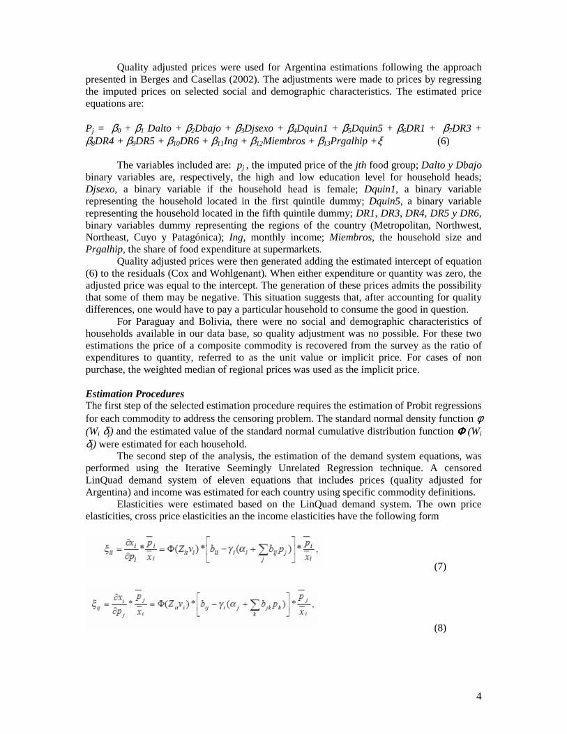
Quality adjusted prices were then generated adding the estimated intercept of equation (6) to the residuals (Cox and Wohlgenant). When either expenditure or quantity was zero, the adjusted price was equal to the intercept. The generation of these prices admits the possibility that some of them may be negative. This situation suggests that, after accounting for quality differences, one would have to pay a particular household to consume the good in question. For Paraguay and Bolivia, there were no social and demographic characteristics of households available in our data base, so quality adjustment was no possible. For these two estimations the price of a composite commodity is recovered from the survey as the ratio of expenditures to quantity, referred to as the unit value or implicit price. For cases of non purchase, the weighted median of regional prices was used as the implicit price. Estimation Procedures The first step of the selected estimation procedure requires the estimation of Probit regressions for each commodity to address the censoring problem. The standard normal density function φ (Wi δj) and the estimated value of the standard normal cumulative distribution function ΦΦΦΦ (Wi δj) were estimated for each household. The second step of the analysis, the estimation of the demand system equations, was performed using the Iterative Seemingly Unrelated Regression technique. A censored LinQuad demand system of eleven equations that includes prices (quality adjusted for Argentina) and income was estimated for each country using specific commodity definitions. Elasticities were estimated based on the LinQuad demand system. The own price elasticities, cross price elasticities an the income elasticities have the following form
(7)
(8)
5
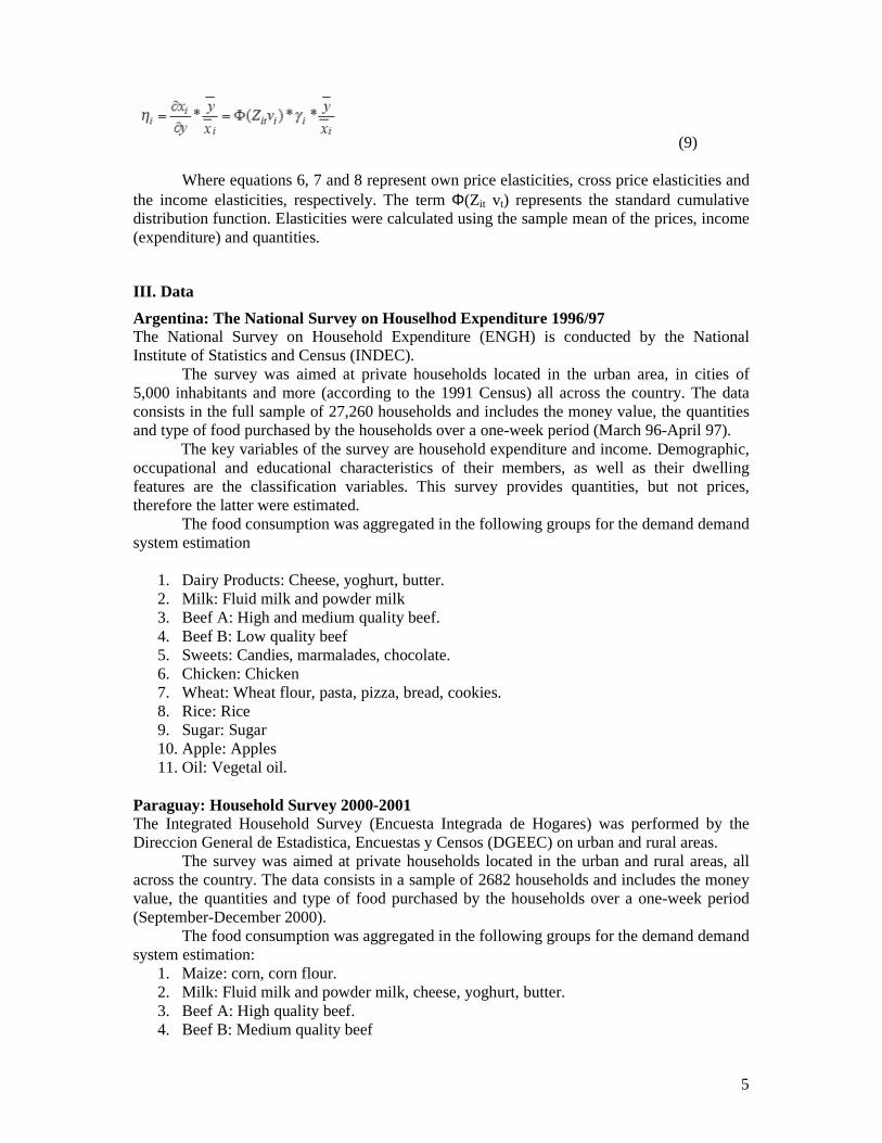
(9) Where equations 6, 7 and 8 represent own price elasticities, cross price elasticities and the income elasticities, respectively. The term Φ(Zit vt) represents the standard cumulative distribution function. Elasticities were calculated using the sample mean of the prices, income (expenditure) and quantities.
III. Data
Argentina: The National Survey on Houselhod Expenditure 1996/97 The National Survey on Household Expenditure (ENGH) is conducted by the National Institute of Statistics and Census (INDEC). The survey was aimed at private households located in the urban area, in cities of 5,000 inhabitants and more (according to the 1991 Census) all across the country. The data consists in the full sample of 27,260 households and includes the money value, the quantities and type of food purchased by the households over a one-week period (March 96-April 97).
The key variables of the survey are household expenditure and income. Demographic, occupational and educational characteristics of their members, as well as their dwelling features are the classification variables. This survey provides quantities, but not prices, therefore the latter were estimated.
The food consumption was aggregated in the following groups for the demand demand system estimation
1. Dairy Products: Cheese, yoghurt, butter. 2. Milk: Fluid milk and powder milk 3. Beef A: High and medium quality beef. 4. Beef B: Low quality beef 5. Sweets: Candies, marmalades, chocolate. 6. Chicken: Chicken 7. Wheat: Wheat flour, pasta, pizza, bread, cookies. 8. Rice: Rice 9. Sugar: Sugar 10. Apple: Apples 11. Oil: Vegetal oil.
Paraguay: Household Survey 2000-2001 The Integrated Household Survey (Encuesta Integrada de Hogares) was performed by the Direccion General de Estadistica, Encuestas y Censos (DGEEC) on urban and rural areas. The survey was aimed at private households located in the urban and rural areas, all across the country. The data consists in a sample of 2682 households and includes the money value, the quantities and type of food purchased by the households over a one-week period (September-December 2000). The food consumption was aggregated in the following groups for the demand demand system estimation:
1. Maize: corn, corn flour. 2. Milk: Fluid milk and powder milk, cheese, yoghurt, butter. 3. Beef A: High quality beef. 4. Beef B: Medium quality beef
6
5. Beef C: Low quality beef. 6. Chicken: Chicken 7. Wheat: Wheat flour, pasta, pizza, bread, cookies. 8. Rice: Rice 9. Sugar: Sugar and brown sugar 10. Apple: Apples 11. Oil: Vegetal oil.
Bolivia: Household Survey 2003-2004 For Bolivia demand estimation the data source is the Household Survey 2003-2004 (Encuesta Continua de Hogares de Bolivia 2003-2004) conducted by the Instituto Nacional de Estadística (INE). The survey was aimed at private households located in urban and rural areas at a national level (nine states) between november 2003 and november 2004. The full data set consists in 9770 households and includes data on quantities and type of food purchased, expenditures, prices and incomes. The data collection was done in two periods, November 2003-March 2004 and May-November 2004. For the econometric estimations the useful sample was reduced to 2983 households after controlling for outliers, inconsistencies and incomplete data. The aggregate food groups are:
1. Maize: corn, corn flour, corn flakes, starch. 2. Milk: fluid milk, powder milk, milk cream, cheese, yoghurt, butter. 3. Beef A: high quality beef. 4. Beef B: medium quality beef 5. Beef C: low quality beef. 6. Chicken: chicken 7. Wheat: wheat flour, pasta, pizza, bread, cookies. 8. Rice: rice 9. Sugar: sugar 10. Apple: Apples 11. Oil: Vegetal oil (sunflower, almond, soybean, olive).
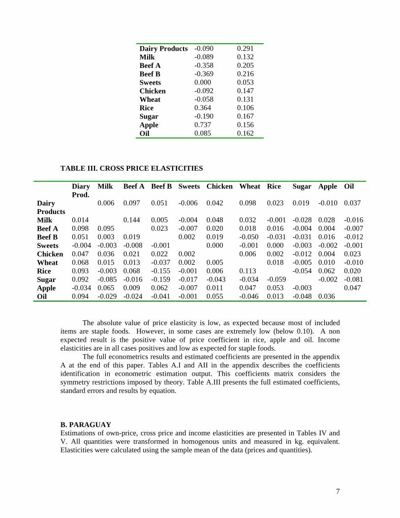
IV. ESTIMATION RESULTS The complete set of estimated coeffients is presented in appendix A, B and C. In the interest of space, the following discussion will focus on the matrix of own and cross price elasticities and income elasticities for each country. A. ARGENTINA Estimations of own-price, cross price and income elasticities are presented in Tables II and III. All quantities were transformed in homogenous units and measured in kg. equivalent. Elasticities were calculated using the sample mean of the data (prices and quantities).
TABLE II. PRICE AND INCOME ELASTICITIES
ELASTICITIES Own Price Income
7
Dairy Products -0.090 0.291 Milk -0.089 0.132 Beef A -0.358 0.205 Beef B -0.369 0.216 Sweets 0.000 0.053 Chicken -0.092 0.147 Wheat -0.058 0.131 Rice 0.364 0.106 Sugar -0.190 0.167 Apple 0.737 0.156 Oil 0.085 0.162
TABLE III. CROSS PRICE ELASTICITIES
Diary Prod.
Milk Beef A Beef B Sweets Chicken Wheat Rice Sugar Apple Oil
Dairy Products
0.006 0.097 0.051 -0.006 0.042 0.098 0.023 0.019 -0.010 0.037
Milk 0.014 0.144 0.005 -0.004 0.048 0.032 -0.001 -0.028 0.028 -0.016 Beef A 0.098 0.095 0.023 -0.007 0.020 0.018 0.016 -0.004 0.004 -0.007 Beef B 0.051 0.003 0.019 0.002 0.019 -0.050 -0.031 -0.031 0.016 -0.012 Sweets -0.004 -0.003 -0.008 -0.001 0.000 -0.001 0.000 -0.003 -0.002 -0.001 Chicken 0.047 0.036 0.021 0.022 0.002 0.006 0.002 -0.012 0.004 0.023 Wheat 0.068 0.015 0.013 -0.037 0.002 0.005 0.018 -0.005 0.010 -0.010 Rice 0.093 -0.003 0.068 -0.155 -0.001 0.006 0.113 -0.054 0.062 0.020 Sugar 0.092 -0.085 -0.016 -0.159 -0.017 -0.043 -0.034 -0.059 -0.002 -0.081 Apple -0.034 0.065 0.009 0.062 -0.007 0.011 0.047 0.053 -0.003 0.047 Oil 0.094 -0.029 -0.024 -0.041 -0.001 0.055 -0.046 0.013 -0.048 0.036
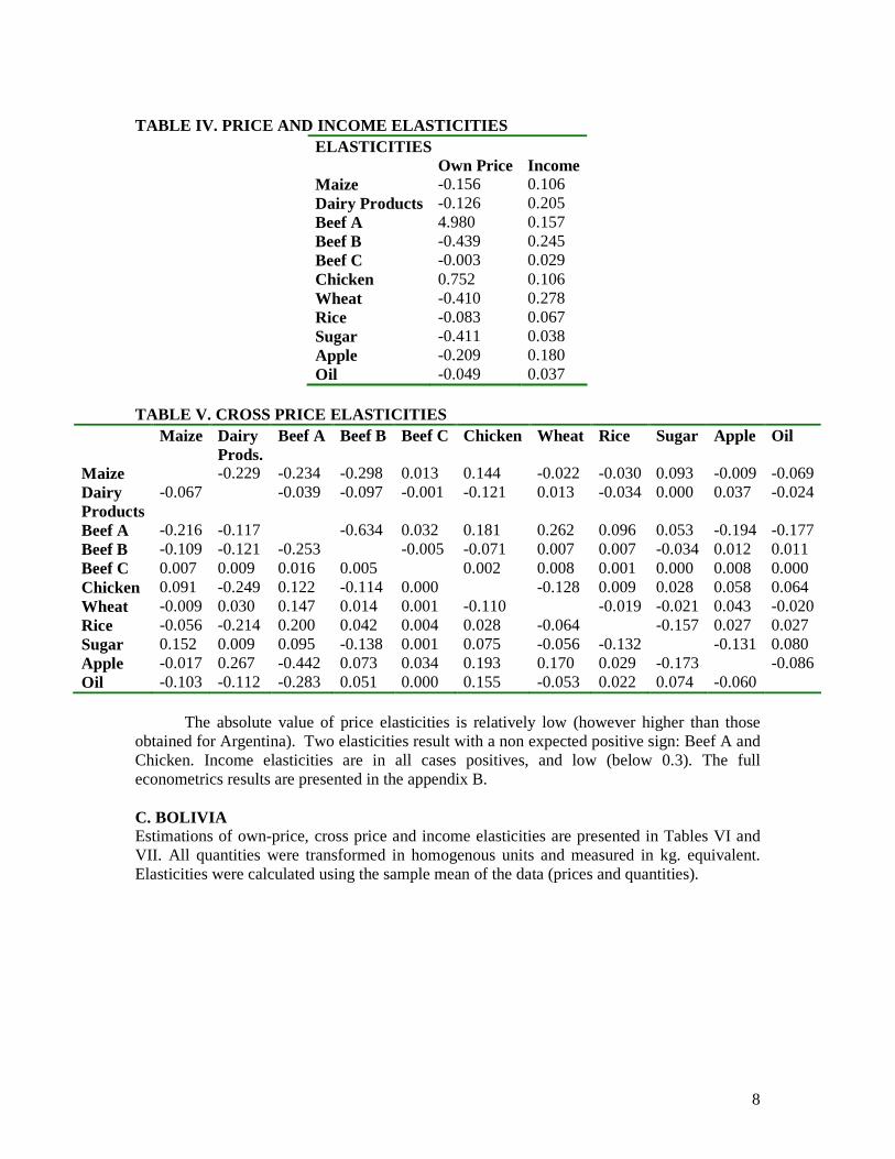
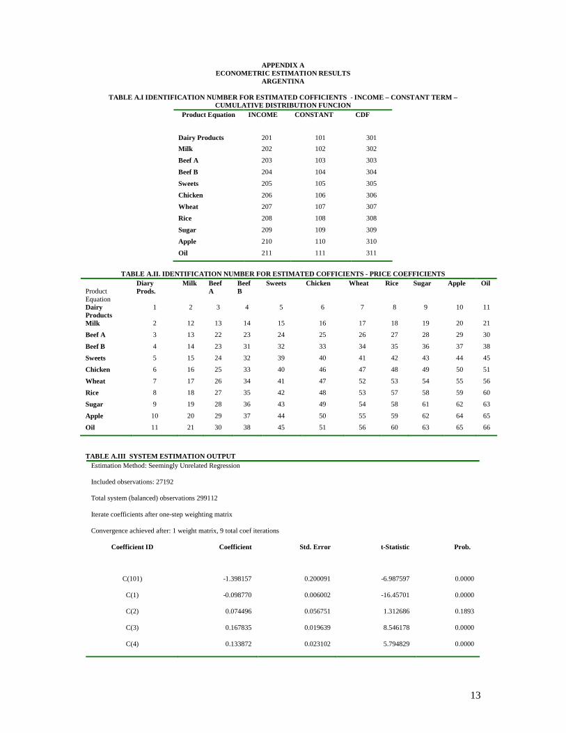
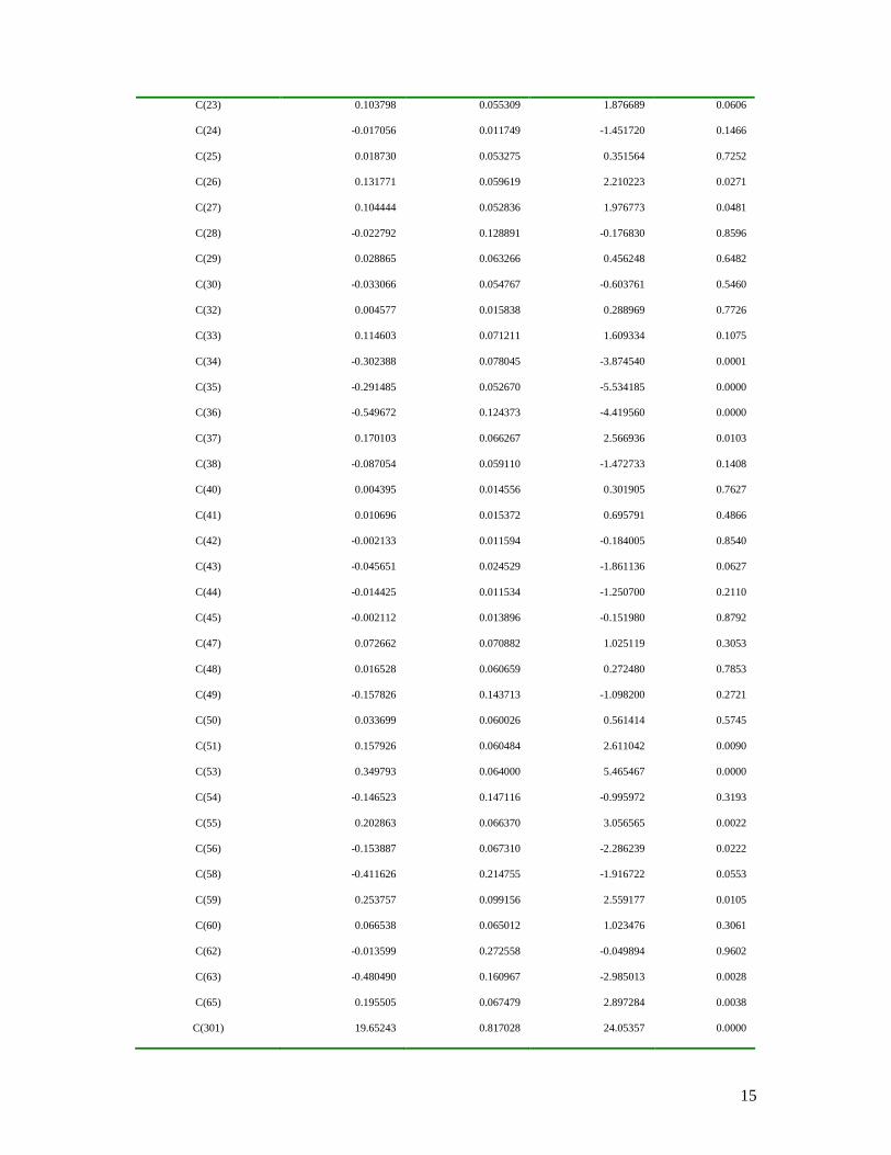
The absolute value of price elasticity is low, as expected because most of included items are staple foods. However, in some cases are extremely low (below 0.10). A non expected result is the positive value of price coefficient in rice, apple and oil. Income elasticities are in all cases positives and low as expected for staple foods. The full econometrics results and estimated coefficients are presented in the appendix A at the end of this paper. Tables A.I and AII in the appendix describes the coefficients identification in econometric estimation output. This coefficients matrix considers the symmetry restrictions imposed by theory. Table A.III presents the full estimated coefficients, standard errors and results by equation. B. PARAGUAY Estimations of own-price, cross price and income elasticities are presented in Tables IV and V. All quantities were transformed in homogenous units and measured in kg. equivalent. Elasticities were calculated using the sample mean of the data (prices and quantities).
8
TABLE IV. PRICE AND INCOME ELASTICITIES
ELASTICITIES Own Price Income Maize -0.156 0.106 Dairy Products -0.126 0.205 Beef A 4.980 0.157 Beef B -0.439 0.245 Beef C -0.003 0.029 Chicken 0.752 0.106 Wheat -0.410 0.278 Rice -0.083 0.067 Sugar -0.411 0.038 Apple -0.209 0.180 Oil -0.049 0.037
TABLE V. CROSS PRICE ELASTICITIES
Maize Dairy Prods.
Beef A Beef B Beef C Chicken Wheat Rice Sugar Apple Oil
Maize -0.229 -0.234 -0.298 0.013 0.144 -0.022 -0.030 0.093 -0.009 -0.069 Dairy Products
-0.067 -0.039 -0.097 -0.001 -0.121 0.013 -0.034 0.000 0.037 -0.024
Beef A -0.216 -0.117 -0.634 0.032 0.181 0.262 0.096 0.053 -0.194 -0.177 Beef B -0.109 -0.121 -0.253 -0.005 -0.071 0.007 0.007 -0.034 0.012 0.011 Beef C 0.007 0.009 0.016 0.005 0.002 0.008 0.001 0.000 0.008 0.000 Chicken 0.091 -0.249 0.122 -0.114 0.000 -0.128 0.009 0.028 0.058 0.064 Wheat -0.009 0.030 0.147 0.014 0.001 -0.110 -0.019 -0.021 0.043 -0.020 Rice -0.056 -0.214 0.200 0.042 0.004 0.028 -0.064 -0.157 0.027 0.027 Sugar 0.152 0.009 0.095 -0.138 0.001 0.075 -0.056 -0.132 -0.131 0.080 Apple -0.017 0.267 -0.442 0.073 0.034 0.193 0.170 0.029 -0.173 -0.086 Oil -0.103 -0.112 -0.283 0.051 0.000 0.155 -0.053 0.022 0.074 -0.060
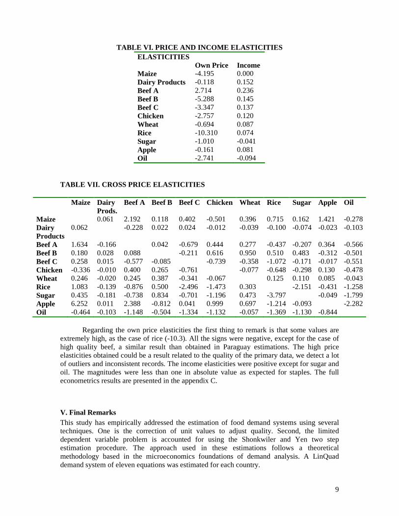
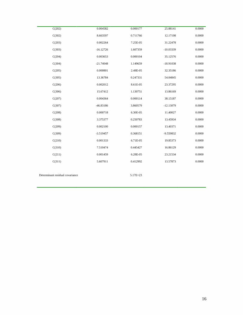
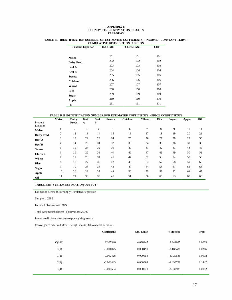
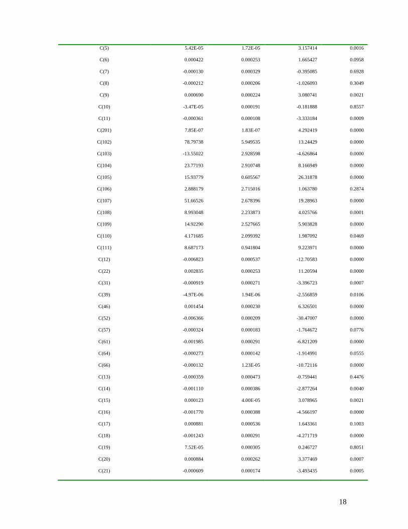
The absolute value of price elasticities is relatively low (however higher than those obtained for Argentina). Two elasticities result with a non expected positive sign: Beef A and Chicken. Income elasticities are in all cases positives, and low (below 0.3). The full econometrics results are presented in the appendix B. C. BOLIVIA Estimations of own-price, cross price and income elasticities are presented in Tables VI and VII. All quantities were transformed in homogenous units and measured in kg. equivalent. Elasticities were calculated using the sample mean of the data (prices and quantities).
9
TABLE VI. PRICE AND INCOME ELASTICITIES ELASTICITIES Own Price Income Maize -4.195 0.000 Dairy Products -0.118 0.152 Beef A 2.714 0.236 Beef B -5.288 0.145 Beef C -3.347 0.137 Chicken -2.757 0.120 Wheat -0.694 0.087 Rice -10.310 0.074 Sugar -1.010 -0.041 Apple -0.161 0.081 Oil -2.741 -0.094
TABLE VII. CROSS PRICE ELASTICITIES
Maize Dairy Prods.
Beef A Beef B Beef C Chicken Wheat Rice Sugar Apple Oil
Maize 0.061 2.192 0.118 0.402 -0.501 0.396 0.715 0.162 1.421 -0.278 Dairy Products
0.062 -0.228 0.022 0.024 -0.012 -0.039 -0.100 -0.074 -0.023 -0.103
Beef A 1.634 -0.166 0.042 -0.679 0.444 0.277 -0.437 -0.207 0.364 -0.566 Beef B 0.180 0.028 0.088 -0.211 0.616 0.950 0.510 0.483 -0.312 -0.501 Beef C 0.258 0.015 -0.577 -0.085 -0.739 -0.358 -1.072 -0.171 -0.017 -0.551 Chicken -0.336 -0.010 0.400 0.265 -0.761 -0.077 -0.648 -0.298 0.130 -0.478 Wheat 0.246 -0.020 0.245 0.387 -0.341 -0.067 0.125 0.110 0.085 -0.043 Rice 1.083 -0.139 -0.876 0.500 -2.496 -1.473 0.303 -2.151 -0.431 -1.258 Sugar 0.435 -0.181 -0.738 0.834 -0.701 -1.196 0.473 -3.797 -0.049 -1.799 Apple 6.252 0.011 2.388 -0.812 0.041 0.999 0.697 -1.214 -0.093 -2.282 Oil -0.464 -0.103 -1.148 -0.504 -1.334 -1.132 -0.057 -1.369 -1.130 -0.844
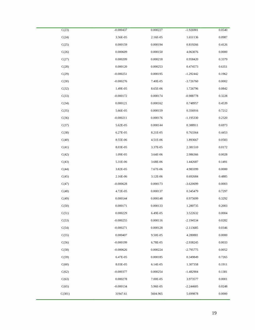
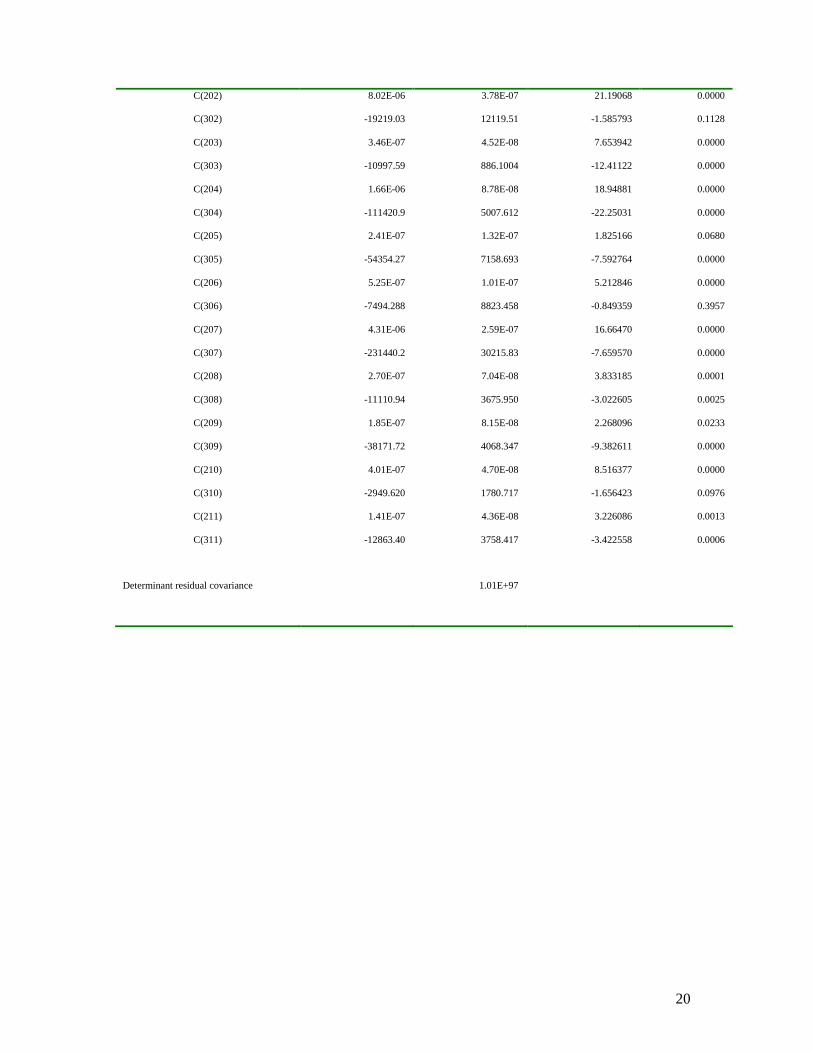
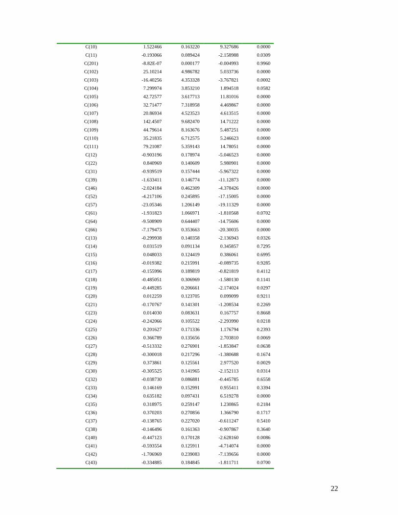
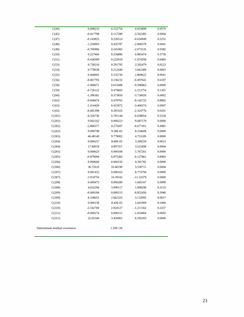
Regarding the own price elasticities the first thing to remark is that some values are extremely high, as the case of rice (-10.3). All the signs were negative, except for the case of high quality beef, a similar result than obtained in Paraguay estimations. The high price elasticities obtained could be a result related to the quality of the primary data, we detect a lot of outliers and inconsistent records. The income elasticities were positive except for sugar and oil. The magnitudes were less than one in absolute value as expected for staples. The full econometrics results are presented in the appendix C.
V. Final Remarks This study has empirically addressed the estimation of food demand systems using several techniques. One is the correction of unit values to adjust quality. Second, the limited dependent variable problem is accounted for using the Shonkwiler and Yen two step estimation procedure. The approach used in these estimations follows a theoretical methodology based in the microeconomics foundations of demand analysis. A LinQuad demand system of eleven equations was estimated for each country.
10
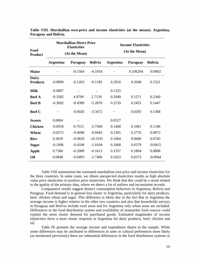
Table VIII. Marshallian own-price and income elasticities (at the means). Argentina, Paraguay and Bolivia.
Marshallian Direct Price Elasticities
(At the Mean)
Income Elasticities
(At the Mean) Food Product
Argentina Paraguay Bolivia Argentina Paraguay Bolivia
Maize - -0.1564 -4.1954 - 0.106294 -0.0002
Dairy Products -0.0899 -0.1263 -0.1185 0.2910 0.2048 0.1521
Milk -0.0887 - - 0.1325
Beef A -0.3585 4.9799 2.7139 0.2049 0.1571 0.2360
Beef B -0.3692 -0.4389 -5.2876 0.2159 0.2455 0.1447
Beef C - -0.0026 -3.3472 - 0.0293 0.1368
Sweets 0.0004 - 0.0527
Chicken -0.0918 0.7515 -2.7569 0.1468 0.1061 0.1196
Wheat -0.0575 -0.4098 -0.6943 0.1305 0.2776 0.0873
Rice 0.3639 -0.0829 -10.3101 0.1064 0.0668 0.0745
Sugar -0.1896 -0.4108 -1.0104 0.1668 0.0379 -0.0415
Apple 0.7366 -0.2089 -0.1613 0.1557 0.1804 0.0808
Oil 0.0848 -0.0493 -2.7406 0.1623 0.0373 -0.0944
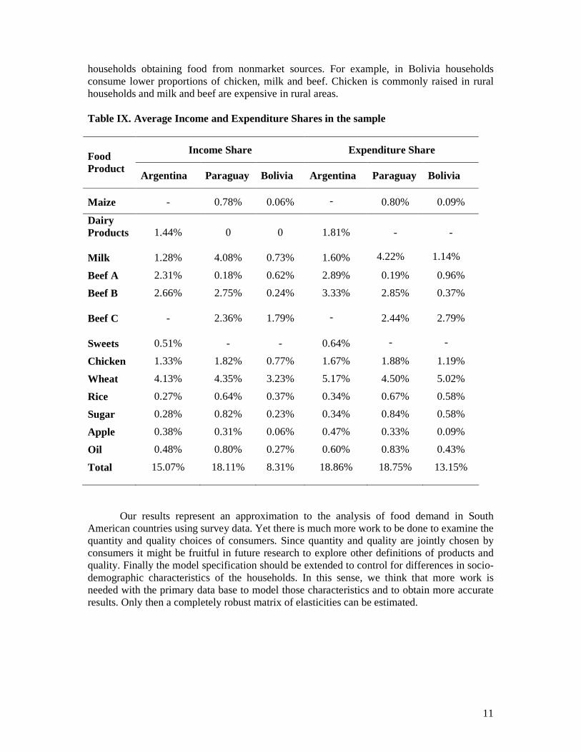
Table VIII summarizes the estimated marshallian own price and income elasticities for the three countries. In some cases, we obtain unexpected elasticities results as high absolute value price elasticities or positive price elasticities. We think that this could be a result related to the quality of the primary data, where we detect a lot of outliers and inconsistent records. Comparative results suggest distinct consumption behaviors in Argentina, Bolivia and Paraguay. Food demand is in general less elastic in Argentina, particularly for dairy products, beef, chicken wheat and sugar. This difference is likely due to the fact that in Argentina the average income is higher relative to the other two countries and also that households surveys in Paraguay and Bolivia include rural areas and for Argentina only urban areas are included. Differences in the food distribution system and availability of nonmarket food sources could explain the more elastic demand for purchased goods. Estimated magnitudes of income elasticities show a more elastic response in Argentina for dairy products, beef, chicken and oil. Table IX presents the average income and expenditure shares in the sample. While some differences may be attributed to differences in taste or cultural preferences more likely (as mentioned previously) there are substantial differences in the food distribution systems or
11
households obtaining food from nonmarket sources. For example, in Bolivia households consume lower proportions of chicken, milk and beef. Chicken is commonly raised in rural households and milk and beef are expensive in rural areas. Table IX. Average Income and Expenditure Shares in the sample
Income Share Expenditure Share Food Product
Argentina Paraguay Bolivia Argentina Paraguay Bolivia
Maize - 0.78% 0.06% - 0.80% 0.09%
Dairy Products 1.44% 0 0 1.81% - -
Milk 1.28% 4.08% 0.73% 1.60% 4.22% 1.14%
Beef A 2.31% 0.18% 0.62% 2.89% 0.19% 0.96%
Beef B 2.66% 2.75% 0.24% 3.33% 2.85% 0.37%
Beef C - 2.36% 1.79% - 2.44% 2.79%
Sweets 0.51% - - 0.64% - -
Chicken 1.33% 1.82% 0.77% 1.67% 1.88% 1.19%
Wheat 4.13% 4.35% 3.23% 5.17% 4.50% 5.02%
Rice 0.27% 0.64% 0.37% 0.34% 0.67% 0.58%
Sugar 0.28% 0.82% 0.23% 0.34% 0.84% 0.58%
Apple 0.38% 0.31% 0.06% 0.47% 0.33% 0.09%
Oil 0.48% 0.80% 0.27% 0.60% 0.83% 0.43%
Total 15.07% 18.11% 8.31% 18.86% 18.75% 13.15%
Our results represent an approximation to the analysis of food demand in South American countries using survey data. Yet there is much more work to be done to examine the quantity and quality choices of consumers. Since quantity and quality are jointly chosen by consumers it might be fruitful in future research to explore other definitions of products and quality. Finally the model specification should be extended to control for differences in socio-demographic characteristics of the households. In this sense, we think that more work is needed with the primary data base to model those characteristics and to obtain more accurate results. Only then a completely robust matrix of elasticities can be estimated.
12
References
Berges, Miriam and Casellas Karina (2002) “A Demand System Analysis of Food for Poor and non Poor Households. The Case Of Argentina” Manuscript, Universidad Nacional de Mar del Plata, Argentina.
Cox, T and Wohlgenant, M (1986) “Prices and Quality Effects in Cross – Sectional Demand Analysis”. American Journal of Agricultural Economics Vol 68 Nro 4. November 1986.
Fabiosa, J. and Helen H. Jensen (2003) “Usefulness of Incomplete Demand Model in Censored Demand System Estimation” American Agricultural Economics Asociation Annual Meeting, Montreal, Quebec, Canada, July 27-30, 2003.
García, Carlos I. (2006) “A Comparative Study Of Household Demand For Meats By U.S. Hispanics” M Sc Thesis Louisiana State University.
Heckman, J.J. (1979) “Sample Selection Bias as a Specification Error.” Econometrica 47:153-162.
Hein, D and Wessells, C (1990) “Demand System Estimation with Microdata: A Censored Regression Approach” Journal of Business And Economics Statistics, July 1990.
Lanfranco, Bruno (2001) “Characteristics Of Hispanic Households’ Demand For Meats: A Comparison With Other Ethnic Groups Utilizing An Incomplete System Of Censored Equations” PhD Dissertation, The University of Georgia.
Lanfranco, Bruno (2004) “Aspectos teóricos y estimación empírica de sistemas de demanda por alimentos”. XXXV Reunión Anual De La Asociación Argentina De Economía Agraria, noviembre de 2004, Mar del Plata, Argentina.
Shonkwiler, J.S. and S.T. Yen (1999) “Two-Step Estimation of a Censored System of Equations.” American Journal of Agricultural Economics. 81(4):972-982.
13
APPENDIX A ECONOMETRIC ESTIMATION RESULTS
ARGENTINA
TABLE A.I IDENTIFICATION NUMBER FOR ESTIMATED COFFI CIENTS - INCOME – CONSTANT TERM – CUMULATIVE DISTRIBUTION FUNCION
Product Equation INCOME CONSTANT CDF
Dairy Products 201 101 301
Milk 202 102 302
Beef A 203 103 303
Beef B 204 104 304
Sweets 205 105 305
Chicken 206 106 306
Wheat 207 107 307
Rice 208 108 308
Sugar 209 109 309
Apple 210 110 310
Oil 211 111 311
TABLE A.II. IDENTIFICATION NUMBER FOR ESTIMATED COF FICIENTS - PRICE COEFFICIENTS
Product Equation
Diary Prods.
Milk Beef A
Beef B
Sweets Chicken Wheat Rice Sugar Apple Oil
Dairy Products
1 2 3 4 5 6 7 8 9 10 11
Milk 2 12 13 14 15 16 17 18 19 20 21
Beef A 3 13 22 23 24 25 26 27 28 29 30
Beef B 4 14 23 31 32 33 34 35 36 37 38
Sweets 5 15 24 32 39 40 41 42 43 44 45
Chicken 6 16 25 33 40 46 47 48 49 50 51
Wheat 7 17 26 34 41 47 52 53 54 55 56
Rice 8 18 27 35 42 48 53 57 58 59 60
Sugar 9 19 28 36 43 49 54 58 61 62 63
Apple 10 20 29 37 44 50 55 59 62 64 65
Oil 11 21 30 38 45 51 56 60 63 65 66
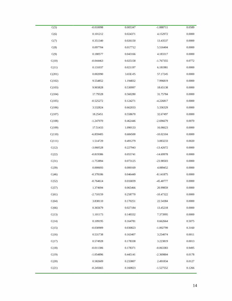
TABLE A.III SYSTEM ESTIMATION OUTPUT
Estimation Method: Seemingly Unrelated Regression
Included observations: 27192
Total system (balanced) observations 299112
Iterate coefficients after one-step weighting matrix
Convergence achieved after: 1 weight matrix, 9 total coef iterations
Coefficient ID Coefficient Std. Error t-Statistic Prob.
C(101) -1.398157 0.200091 -6.987597 0.0000
C(1) -0.098770 0.006002 -16.45701 0.0000
C(2) 0.074496 0.056751 1.312686 0.1893
C(3) 0.167835 0.019639 8.546178 0.0000
C(4) 0.133872 0.023102 5.794829 0.0000
14
C(5) -0.010098 0.005347 -1.888711 0.0589
C(6) 0.101212 0.024371 4.152972 0.0000
C(7) 0.351340 0.026150 13.43537 0.0000
C(8) 0.097704 0.017712 5.516404 0.0000
C(9) 0.180577 0.043166 4.183317 0.0000
C(10) -0.044463 0.025158 -1.767355 0.0772
C(11) 0.131037 0.021197 6.181981 0.0000
C(201) 0.002090 3.65E-05 57.17245 0.0000
C(102) 9.554852 1.194832 7.996819 0.0000
C(103) 9.903828 0.530997 18.65138 0.0000
C(104) 17.79328 0.560280 31.75784 0.0000
C(105) -0.525272 0.124271 -4.226817 0.0000
C(106) 3.532824 0.662033 5.336329 0.0000
C(107) 18.25451 0.558670 32.67497 0.0000
C(108) -1.247070 0.462446 -2.696679 0.0070
C(109) 17.51433 1.090133 16.06623 0.0000
C(110) -6.859405 0.684500 -10.02104 0.0000
C(111) 1.514729 0.491279 3.083233 0.0020
C(12) -3.060528 0.227943 -13.42672 0.0000
C(22) -0.819386 0.055741 -14.69978 0.0000
C(31) -1.753894 0.073125 -23.98503 0.0000
C(39) 0.000693 0.000169 4.089452 0.0000
C(46) -0.378186 0.046449 -8.141875 0.0000
C(52) -0.764614 0.016839 -45.40777 0.0000
C(57) 1.374694 0.065466 20.99859 0.0000
C(61) -2.710159 0.258770 -10.47322 0.0000
C(64) 3.838110 0.170251 22.54384 0.0000
C(66) 0.365679 0.027184 13.45218 0.0000
C(13) 1.101173 0.149332 7.373995 0.0000
C(14) 0.109195 0.164781 0.662664 0.5075
C(15) -0.030909 0.030823 -1.002799 0.3160
C(16) 0.531738 0.163407 3.254074 0.0011
C(17) 0.574928 0.178338 3.223819 0.0013
C(18) -0.011306 0.178371 -0.063383 0.9495
C(19) -1.054896 0.445141 -2.369804 0.0178
C(20) 0.582609 0.233807 2.491834 0.0127
C(21) -0.245665 0.160823 -1.527552 0.1266
15
C(23) 0.103798 0.055309 1.876689 0.0606
C(24) -0.017056 0.011749 -1.451720 0.1466
C(25) 0.018730 0.053275 0.351564 0.7252
C(26) 0.131771 0.059619 2.210223 0.0271
C(27) 0.104444 0.052836 1.976773 0.0481
C(28) -0.022792 0.128891 -0.176830 0.8596
C(29) 0.028865 0.063266 0.456248 0.6482
C(30) -0.033066 0.054767 -0.603761 0.5460
C(32) 0.004577 0.015838 0.288969 0.7726
C(33) 0.114603 0.071211 1.609334 0.1075
C(34) -0.302388 0.078045 -3.874540 0.0001
C(35) -0.291485 0.052670 -5.534185 0.0000
C(36) -0.549672 0.124373 -4.419560 0.0000
C(37) 0.170103 0.066267 2.566936 0.0103
C(38) -0.087054 0.059110 -1.472733 0.1408
C(40) 0.004395 0.014556 0.301905 0.7627
C(41) 0.010696 0.015372 0.695791 0.4866
C(42) -0.002133 0.011594 -0.184005 0.8540
C(43) -0.045651 0.024529 -1.861136 0.0627
C(44) -0.014425 0.011534 -1.250700 0.2110
C(45) -0.002112 0.013896 -0.151980 0.8792
C(47) 0.072662 0.070882 1.025119 0.3053
C(48) 0.016528 0.060659 0.272480 0.7853
C(49) -0.157826 0.143713 -1.098200 0.2721
C(50) 0.033699 0.060026 0.561414 0.5745
C(51) 0.157926 0.060484 2.611042 0.0090
C(53) 0.349793 0.064000 5.465467 0.0000
C(54) -0.146523 0.147116 -0.995972 0.3193
C(55) 0.202863 0.066370 3.056565 0.0022
C(56) -0.153887 0.067310 -2.286239 0.0222
C(58) -0.411626 0.214755 -1.916722 0.0553
C(59) 0.253757 0.099156 2.559177 0.0105
C(60) 0.066538 0.065012 1.023476 0.3061
C(62) -0.013599 0.272558 -0.049894 0.9602
C(63) -0.480490 0.160967 -2.985013 0.0028
C(65) 0.195505 0.067479 2.897284 0.0038
C(301) 19.65243 0.817028 24.05357 0.0000
16
C(202) 0.004582 0.000177 25.88141 0.0000
C(302) 8.663597 0.711766 12.17198 0.0000
C(203) 0.002264 7.25E-05 31.22478 0.0000
C(303) -16.12726 1.607359 -10.03339 0.0000
C(204) 0.003653 0.000104 35.12576 0.0000
C(304) -21.74048 1.149659 -18.91038 0.0000
C(205) 0.000801 2.48E-05 32.35186 0.0000
C(305) 13.36784 0.247331 54.04845 0.0000
C(206) 0.002012 8.61E-05 23.37295 0.0000
C(306) 15.67412 1.130751 13.86169 0.0000
C(207) 0.004364 0.000114 38.15187 0.0000
C(307) -46.83186 3.860579 -12.13079 0.0000
C(208) 0.000718 6.30E-05 11.40027 0.0000
C(308) 3.375377 0.250783 13.45934 0.0000
C(209) 0.002100 0.000157 13.40371 0.0000
C(309) -3.519457 0.368151 -9.559832 0.0000
C(210) 0.001333 6.71E-05 19.85373 0.0000
C(310) 7.510474 0.445427 16.86129 0.0000
C(211) 0.001459 6.28E-05 23.21534 0.0000
C(311) 5.607911 0.412992 13.57873 0.0000
Determinant residual covariance 5.17E+23
17
APPENDIX B ECONOMETRIC ESTIMATION RESULTS
PARAGUAY
TABLE B.I IDENTIFICATION NUMBER FOR ESTIMATED COFF ICIENTS - INCOME – CONSTANT TERM – CUMULATIVE DISTRIBUTION FUNCION
Product Equation INCOME CONSTANT CDF
Maize 201 101 301
Dairy Prod. 202 102 302
Beef A 203 103 303
Beef B 204 104 304
Sweets 205 105 305
Chicken 206 106 306
Wheat 207 107 307
Rice 208 108 308
Sugar 209 109 309
Apple 210 110 310
Oil 211 111 311
TABLE B.II IDENTIFICATION NUMBER FOR ESTIMATED COFF ICIENTS - PRICE COEFFICIENTS Product Equation
Maize Dairy Prods.
Beef A
Beef B
Sweets Chicken Wheat Rice Sugar Apple Oil
Maize 1 2 3 4 5 6 7 8 9 10 11
Dairy Prod. 2 12 13 14 15 16 17 18 19 20 21
Beef A 3 13 22 23 24 25 26 27 28 29 30
Beef B 4 14 23 31 32 33 34 35 36 37 38
Sweets 5 15 24 32 39 40 41 42 43 44 45
Chicken 6 16 25 33 40 46 47 48 49 50 51
Wheat 7 17 26 34 41 47 52 53 54 55 56
Rice 8 18 27 35 42 48 53 57 58 59 60
Sugar 9 19 28 36 43 49 54 58 61 62 63
Apple 10 20 29 37 44 50 55 59 62 64 65
Oil 11 21 30 38 45 51 56 60 63 65 66
TABLE B.III SYSTEM ESTIMATION OUTPUT Estimation Method: Seemingly Unrelated Regression
Sample: 1 2682
Included observations: 2674
Total system (unbalanced) observations 29392
Iterate coefficients after one-step weighting matrix
Convergence achieved after: 1 weight matrix, 10 total coef iterations
Coefficient Std. Error t-Statistic Prob.
C(101) 12.05546 4.098147 2.941685 0.0033
C(1) -0.001075 0.000491 -2.188488 0.0286
C(2) -0.002428 0.000653 -3.720538 0.0002
C(3) -0.000443 0.000304 -1.458729 0.1447
C(4) -0.000684 0.000270 -2.537989 0.0112
18
C(5) 5.42E-05 1.72E-05 3.157414 0.0016
C(6) 0.000422 0.000253 1.665427 0.0958
C(7) -0.000130 0.000329 -0.395085 0.6928
C(8) -0.000212 0.000206 -1.026093 0.3049
C(9) 0.000690 0.000224 3.080741 0.0021
C(10) -3.47E-05 0.000191 -0.181888 0.8557
C(11) -0.000361 0.000108 -3.333184 0.0009
C(201) 7.85E-07 1.83E-07 4.292419 0.0000
C(102) 78.79738 5.949535 13.24429 0.0000
C(103) -13.55022 2.928598 -4.626864 0.0000
C(104) 23.77193 2.910748 8.166949 0.0000
C(105) 15.93779 0.605567 26.31878 0.0000
C(106) 2.888179 2.715016 1.063780 0.2874
C(107) 51.66526 2.678396 19.28963 0.0000
C(108) 8.993048 2.233873 4.025766 0.0001
C(109) 14.92290 2.527665 5.903828 0.0000
C(110) 4.171685 2.099392 1.987092 0.0469
C(111) 8.687173 0.941804 9.223971 0.0000
C(12) -0.006823 0.000537 -12.70583 0.0000
C(22) 0.002835 0.000253 11.20594 0.0000
C(31) -0.000919 0.000271 -3.396723 0.0007
C(39) -4.97E-06 1.94E-06 -2.556859 0.0106
C(46) 0.001454 0.000230 6.326501 0.0000
C(52) -0.006366 0.000209 -30.47007 0.0000
C(57) -0.000324 0.000183 -1.764672 0.0776
C(61) -0.001985 0.000291 -6.821209 0.0000
C(64) -0.000273 0.000142 -1.914991 0.0555
C(66) -0.000132 1.23E-05 -10.72116 0.0000
C(13) -0.000359 0.000473 -0.759441 0.4476
C(14) -0.001110 0.000386 -2.877264 0.0040
C(15) 0.000123 4.00E-05 3.078965 0.0021
C(16) -0.001770 0.000388 -4.566197 0.0000
C(17) 0.000881 0.000536 1.643361 0.1003
C(18) -0.001243 0.000291 -4.271719 0.0000
C(19) 7.52E-05 0.000305 0.246727 0.8051
C(20) 0.000884 0.000262 3.377469 0.0007
C(21) -0.000609 0.000174 -3.493435 0.0005
19
C(23) -0.000437 0.000227 -1.926901 0.0540
C(24) 3.56E-05 2.16E-05 1.651136 0.0987
C(25) 0.000159 0.000194 0.819266 0.4126
C(26) 0.000609 0.000150 4.063076 0.0000
C(27) 0.000209 0.000218 0.958420 0.3379
C(28) 0.000120 0.000253 0.474573 0.6351
C(29) -0.000251 0.000195 -1.292442 0.1962
C(30) -0.000276 7.40E-05 -3.726760 0.0002
C(32) 1.49E-05 8.65E-06 1.726796 0.0842
C(33) -0.000172 0.000174 -0.988778 0.3228
C(34) 0.000121 0.000162 0.748957 0.4539
C(35) 5.66E-05 0.000159 0.356916 0.7212
C(36) -0.000211 0.000176 -1.195330 0.2320
C(37) 5.62E-05 0.000144 0.388911 0.6973
C(38) 6.27E-05 8.21E-05 0.763364 0.4453
C(40) 8.55E-06 4.51E-06 1.893667 0.0583
C(41) 8.03E-05 3.37E-05 2.381510 0.0172
C(42) 1.09E-05 3.64E-06 2.986366 0.0028
C(43) 5.31E-06 3.68E-06 1.442687 0.1491
C(44) 3.82E-05 7.67E-06 4.983399 0.0000
C(45) 2.16E-06 3.12E-06 0.692684 0.4885
C(47) -0.000628 0.000173 -3.620699 0.0003
C(48) 4.72E-05 0.000137 0.345479 0.7297
C(49) 0.000144 0.000148 0.975699 0.3292
C(50) 0.000171 0.000133 1.280735 0.2003
C(51) 0.000229 6.49E-05 3.522632 0.0004
C(53) -0.000255 0.000116 -2.194534 0.0282
C(54) -0.000271 0.000128 -2.113685 0.0346
C(55) 0.000407 9.50E-05 4.280881 0.0000
C(56) -0.000199 6.78E-05 -2.938245 0.0033
C(58) -0.000626 0.000224 -2.795775 0.0052
C(59) 6.47E-05 0.000185 0.349849 0.7265
C(60) 8.03E-05 6.14E-05 1.307358 0.1911
C(62) -0.000377 0.000254 -1.482904 0.1381
C(63) 0.000278 7.00E-05 3.973577 0.0001
C(65) -0.000134 5.96E-05 -2.244605 0.0248
C(301) 31947.61 5604.965 5.699878 0.0000
20
C(202) 8.02E-06 3.78E-07 21.19068 0.0000
C(302) -19219.03 12119.51 -1.585793 0.1128
C(203) 3.46E-07 4.52E-08 7.653942 0.0000
C(303) -10997.59 886.1004 -12.41122 0.0000
C(204) 1.66E-06 8.78E-08 18.94881 0.0000
C(304) -111420.9 5007.612 -22.25031 0.0000
C(205) 2.41E-07 1.32E-07 1.825166 0.0680
C(305) -54354.27 7158.693 -7.592764 0.0000
C(206) 5.25E-07 1.01E-07 5.212846 0.0000
C(306) -7494.288 8823.458 -0.849359 0.3957
C(207) 4.31E-06 2.59E-07 16.66470 0.0000
C(307) -231440.2 30215.83 -7.659570 0.0000
C(208) 2.70E-07 7.04E-08 3.833185 0.0001
C(308) -11110.94 3675.950 -3.022605 0.0025
C(209) 1.85E-07 8.15E-08 2.268096 0.0233
C(309) -38171.72 4068.347 -9.382611 0.0000
C(210) 4.01E-07 4.70E-08 8.516377 0.0000
C(310) -2949.620 1780.717 -1.656423 0.0976
C(211) 1.41E-07 4.36E-08 3.226086 0.0013
C(311) -12863.40 3758.417 -3.422558 0.0006
Determinant residual covariance 1.01E+97
21
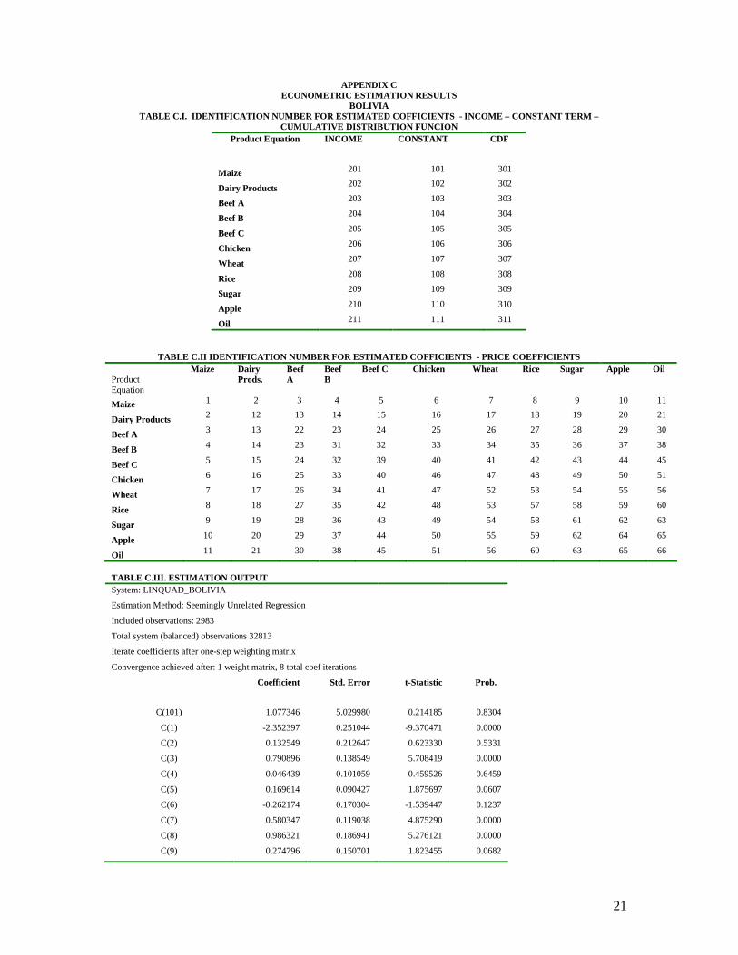
APPENDIX C ECONOMETRIC ESTIMATION RESULTS
BOLIVIA TABLE C.I. IDENTIFICATION NUMBER FOR ESTIMATED COF FICIENTS - INCOME – CONSTANT TERM –
CUMULATIVE DISTRIBUTION FUNCION Product Equation INCOME CONSTANT CDF
Maize 201 101 301
Dairy Products 202 102 302
Beef A 203 103 303
Beef B 204 104 304
Beef C 205 105 305
Chicken 206 106 306
Wheat 207 107 307
Rice 208 108 308
Sugar 209 109 309
Apple 210 110 310
Oil 211 111 311
TABLE C.II IDENTIFICATION NUMBER FOR ESTIMATED COFF ICIENTS - PRICE COEFFICIENTS Product Equation
Maize Dairy Prods.
Beef A
Beef B
Beef C Chicken Wheat Rice Sugar Apple Oil
Maize 1 2 3 4 5 6 7 8 9 10 11
Dairy Products 2 12 13 14 15 16 17 18 19 20 21
Beef A 3 13 22 23 24 25 26 27 28 29 30
Beef B 4 14 23 31 32 33 34 35 36 37 38
Beef C 5 15 24 32 39 40 41 42 43 44 45
Chicken 6 16 25 33 40 46 47 48 49 50 51
Wheat 7 17 26 34 41 47 52 53 54 55 56
Rice 8 18 27 35 42 48 53 57 58 59 60
Sugar 9 19 28 36 43 49 54 58 61 62 63
Apple 10 20 29 37 44 50 55 59 62 64 65
Oil 11 21 30 38 45 51 56 60 63 65 66
TABLE C.III. ESTIMATION OUTPUT System: LINQUAD_BOLIVIA
Estimation Method: Seemingly Unrelated Regression
Included observations: 2983
Total system (balanced) observations 32813
Iterate coefficients after one-step weighting matrix
Convergence achieved after: 1 weight matrix, 8 total coef iterations
Coefficient Std. Error t-Statistic Prob.
C(101) 1.077346 5.029980 0.214185 0.8304
C(1) -2.352397 0.251044 -9.370471 0.0000
C(2) 0.132549 0.212647 0.623330 0.5331
C(3) 0.790896 0.138549 5.708419 0.0000
C(4) 0.046439 0.101059 0.459526 0.6459
C(5) 0.169614 0.090427 1.875697 0.0607
C(6) -0.262174 0.170304 -1.539447 0.1237
C(7) 0.580347 0.119038 4.875290 0.0000
C(8) 0.986321 0.186941 5.276121 0.0000
C(9) 0.274796 0.150701 1.823455 0.0682
22
C(10) 1.522466 0.163220 9.327686 0.0000
C(11) -0.193066 0.089424 -2.158988 0.0309
C(201) -8.82E-07 0.000177 -0.004993 0.9960
C(102) 25.10214 4.986782 5.033736 0.0000
C(103) -16.40256 4.353328 -3.767821 0.0002
C(104) 7.299974 3.853210 1.894518 0.0582
C(105) 42.72577 3.617713 11.81016 0.0000
C(106) 32.71477 7.318958 4.469867 0.0000
C(107) 20.86934 4.523523 4.613515 0.0000
C(108) 142.4507 9.682470 14.71222 0.0000
C(109) 44.79614 8.163676 5.487251 0.0000
C(110) 35.21835 6.712575 5.246623 0.0000
C(111) 79.21087 5.359143 14.78051 0.0000
C(12) -0.903196 0.178974 -5.046523 0.0000
C(22) 0.840969 0.140609 5.980901 0.0000
C(31) -0.939519 0.157444 -5.967322 0.0000
C(39) -1.633411 0.146774 -11.12873 0.0000
C(46) -2.024184 0.462309 -4.378426 0.0000
C(52) -4.217106 0.245895 -17.15005 0.0000
C(57) -23.05346 1.206149 -19.11329 0.0000
C(61) -1.931823 1.066971 -1.810568 0.0702
C(64) -9.508909 0.644407 -14.75606 0.0000
C(66) -7.179473 0.353663 -20.30035 0.0000
C(13) -0.299938 0.140358 -2.136943 0.0326
C(14) 0.031519 0.091134 0.345857 0.7295
C(15) 0.048033 0.124419 0.386061 0.6995
C(16) -0.019382 0.215991 -0.089735 0.9285
C(17) -0.155996 0.189819 -0.821819 0.4112
C(18) -0.485051 0.306969 -1.580130 0.1141
C(19) -0.449285 0.206661 -2.174024 0.0297
C(20) 0.012259 0.123705 0.099099 0.9211
C(21) -0.170767 0.141301 -1.208534 0.2269
C(23) 0.014030 0.083631 0.167757 0.8668
C(24) -0.242066 0.105522 -2.293990 0.0218
C(25) 0.201627 0.171336 1.176794 0.2393
C(26) 0.366789 0.135656 2.703810 0.0069
C(27) -0.513332 0.276901 -1.853847 0.0638
C(28) -0.300018 0.217296 -1.380688 0.1674
C(29) 0.373861 0.125561 2.977520 0.0029
C(30) -0.305525 0.141965 -2.152113 0.0314
C(32) -0.038730 0.086881 -0.445785 0.6558
C(33) 0.146169 0.152991 0.955411 0.3394
C(34) 0.635182 0.097431 6.519278 0.0000
C(35) 0.318975 0.259147 1.230865 0.2184
C(36) 0.370203 0.270856 1.366790 0.1717
C(37) -0.138765 0.227020 -0.611247 0.5410
C(38) -0.146496 0.161363 -0.907867 0.3640
C(40) -0.447123 0.170128 -2.628160 0.0086
C(41) -0.593554 0.125911 -4.714074 0.0000
C(42) -1.706969 0.239083 -7.139656 0.0000
C(43) -0.334885 0.184845 -1.811711 0.0700
23
C(44) 0.008233 0.152754 0.053899 0.9570
C(45) -0.417798 0.117280 -3.562385 0.0004
C(47) -0.143825 0.226514 -0.634949 0.5255
C(48) -1.250003 0.435787 -2.868378 0.0041
C(49) -0.706906 0.341083 -2.072535 0.0382
C(50) 0.227466 0.256886 0.885474 0.3759
C(51) -0.438399 0.222019 -1.974599 0.0483
C(53) 0.730210 0.291795 2.502479 0.0123
C(54) 0.778038 0.212440 3.662389 0.0003
C(55) 0.446902 0.155736 2.869622 0.0041
C(56) -0.067795 0.136232 -0.497641 0.6187
C(58) -5.908671 0.615688 -9.596863 0.0000
C(59) -0.726122 0.479683 -1.513754 0.1301
C(60) -1.396301 0.373850 -3.734926 0.0002
C(62) -0.068474 0.479765 -0.142725 0.8865
C(63) -1.414420 0.415972 -3.400274 0.0007
C(65) -0.681398 0.293103 -2.324776 0.0201
C(301) -4.326736 6.781144 -0.638054 0.5234
C(202) 0.002162 0.000223 9.687179 0.0000
C(302) -2.896577 4.275697 -0.677451 0.4981
C(203) 0.000798 9.58E-05 8.334608 0.0000
C(303) 46.48140 9.779002 4.753185 0.0000
C(204) 0.000257 8.00E-05 3.209259 0.0013
C(304) 17.60018 4.997357 3.521898 0.0004
C(205) 0.000623 0.000108 5.767261 0.0000
C(305) -0.879094 6.875383 -0.127861 0.8983
C(206) 0.000660 0.000150 4.391781 0.0000
C(306) 36.72610 10.40190 3.530711 0.0004
C(207) 0.001432 0.000163 8.774794 0.0000
C(307) -119.8756 10.39342 -11.53379 0.0000
C(208) 0.000475 0.000289 1.645167 0.0999
C(308) 4.032294 3.999117 1.008296 0.3133
C(209) -0.000184 0.000215 -0.852456 0.3940
C(309) 8.338655 2.662325 3.132095 0.0017
C(210) 0.000138 8.42E-05 1.641909 0.1006
C(310) -3.542760 2.924127 -1.211562 0.2257
C(211) -0.000274 0.000151 -1.816804 0.0693
C(311) 22.05349 3.450061 6.392203 0.0000
Determinant residual covariance 1.59E+26