Embed Size (px)
Citation preview
1
An Introduction to Model Predictive Control
TEQIP Workshop, IIT Kanpur
22’nd Sept., 2016
Sachin C. Patwardhan
Dept. of Chemical Engineering
I.I.T. Bombay
Email: [email protected]
Automation LabIIT Bombay
22
Outline
Motivation
Development of MPC Relevant Linear Models
Review of Linear Quadratic Optimal Control
Linear Model Predictive Control Formulation
Adaptive MPC
Nonlinear Model Predictive Control Formulation
Summary and Research Directions
Automation LabIIT Bombay
33
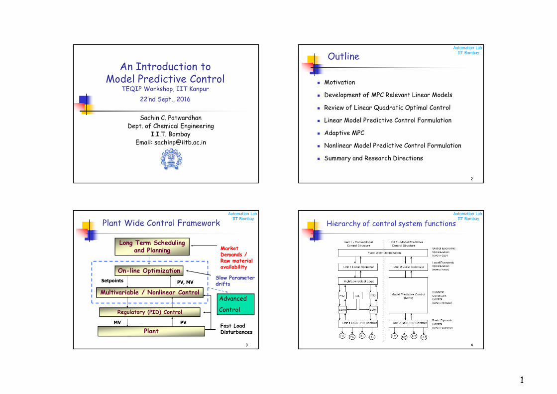
Long Term Scheduling and Planning
On-line Optimization
Multivariable / Nonlinear Control
Regulatory (PID) Control
Plant
Slow Parameter drifts
MarketDemands /Raw materialavailability
MVFast Load Disturbances
PV
Advanced
Control
Setpoints PV, MV
Plant Wide Control Framework
Automation LabIIT Bombay
44
Hierarchy of control system functions
2
Automation LabIIT Bombay
55
Why Multi-Variable Control?
Most rear systems have multiple inputs and
multiple controlled outputs
Systems exhibit complex and multi-variable
interactions between inputs and outputs variables
Need to operate a system within operating
constraints
Safety limits
Input saturation constraints
Product quality constraints
Automation LabIIT Bombay
66
Why Model Predictive Control?
Need to control over wide operating range
Process nonlinearities
Changing process parameters / conditions
Conventional approach : Multi-loop PI - difficult to tune
Ad-hoc constraint handling using logic programming
(PLCs): lack of coordination
MPC deals with multivariable interactions,
operating constraints, and process nonlinearity
systematically
Automation LabIIT Bombay
77
Model Predictive Control
Most widely used multivariable control scheme in
the process industries over last 35 years
Used for controlling critical unit operations (such as
reactors) in refineries world over
With increasing computing power, MPC is
increasingly being applied in diverse application
areas: robotics, fuel cells, internet search engines,
planning and scheduling, control of drives, bio-
medical applications
Automation LabIIT Bombay
8
Development of MPC Relevant Linear Perturbation Models
3
Automation LabIIT Bombay
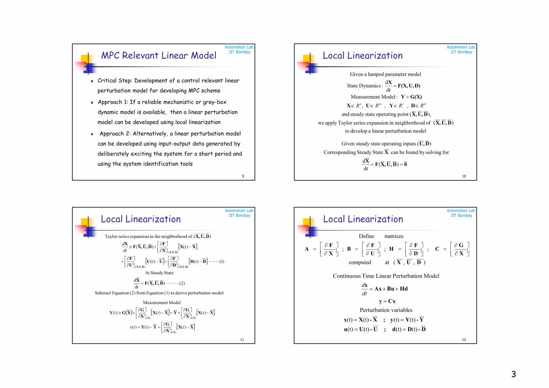
MPC Relevant Linear Model
Critical Step: Development of a control relevant linear
perturbation model for developing MPC scheme
Approach 1: If a reliable mechanistic or grey-box
dynamic model is available, then a linear perturbation
model can be developed using local linearization
Approach 2: Alternatively, a linear perturbation model
can be developed using input-output data generated by
deliberately exciting the system for a short period and
using the system identification tools
9
Automation LabIIT Bombay
10
Local Linearization
modelon perturbatilinear a develop to
)( of odneighborhoin expansion seriesTaylor apply we
),(point operating statesteady and
,,,
:Modelt Measuremen
dt
d :Dynamics State
modelparameter lumped aGiven
D,U,X
D,U,X
DYUX
G(X)Y
D)U,F(X,X
drmn RRRR
0D,U,XFX
X
D,U
)(dt
d
for solvingby found becan StateSteady ingCorrespond
)( inputs operating statesteady Given
Automation LabIIT Bombay
11
Local Linearization
modelon perturbati derive to(1)Equation from (2)Equation Subsract
)2()(dt
d
StateSteady At
)1()()(
)()(
)( of odneighborho in theexpansion seriesTaylor
)()(
)(
D,U,XFX
DDD
FUU
U
F
XXX
FD,U,XF
X
D,U,X
D,U,XD,U,X
D,U,X
tt
tdt
d
XXX
GYY
XXX
GYXX
X
GXGY
X
XX
)()()(
)()()(
Modelt Measuremen
)(
)()(
ttty
ttt
Automation LabIIT Bombay
12
Local Linearization
D-Dd ;U-Uu
Y-Yy;X-Xx
Cxy
HdBuAxx
(t)(t)(t)(t)
(t)(t)(t)(t)
eson variablPerturbati
Modelon PerturbatiLinear Time Continuous
dt
d
),,(at computed
;;;
matrices Define
DUX
X
GC
D
FH
U
FB
X
FA
4
Automation LabIIT Bombay
13
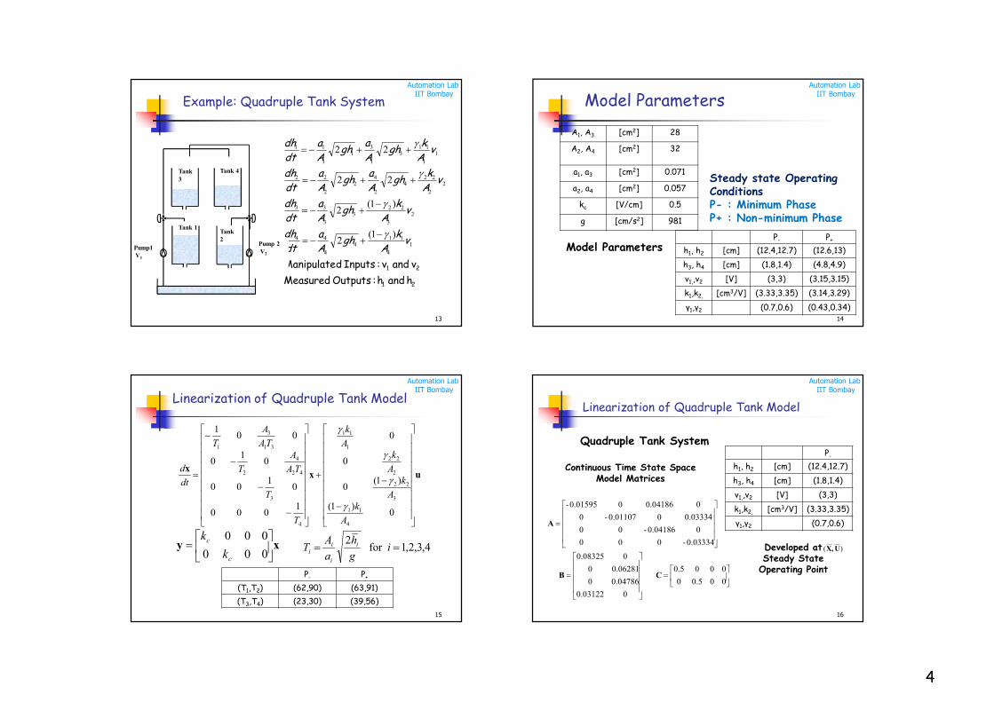
Example: Quadruple Tank System
21
21
h and h :Outputs Measured
v and v :Inputs dManipulate
1
4
114
4
44
2
3
223
3
33
2
2
224
2
42
2
22
1
1
113
1
31
1
11
)1(2
)1(2
22
22
vA
kgh
A
a
dt
dh
vA
kgh
A
a
dt
dh
vA
kgh
A
agh
A
a
dt
dh
vA
kgh
A
agh
A
a
dt
dh
Pump 2V2
Pump1V1
Tank3
Tank 2
Tank 1
Tank 4
Automation LabIIT Bombay
Model Parameters
14
Steady state Operating ConditionsP- : Minimum Phase P+ : Non-minimum Phase
A1, A3 [cm2] 28
A2, A4 [cm2] 32
a1, a3 [cm2] 0.071
a2, a4 [cm2] 0.057
kc [V/cm] 0.5
g [cm/s2] 981
P- P+
h1, h2 [cm] (12.4,12.7) (12.6,13)
h3, h4 [cm] (1.8,1.4) (4.8,4.9)
v1,,v2 [V] (3,3) (3.15,3.15)
k1,k2, [cm3/V] (3.33,3.35) (3.14,3.29)
γ1,γ2 (0.7,0.6) (0.43,0.34)
Model Parameters
Automation LabIIT Bombay
Linearization of Quadruple Tank Model
15
uxx
0)1(
)1(0
0
0
1000
01
00
01
0
001
4
11
3
22
2
22
1
11
4
3
42
4
2
31
3
1
A
kA
kA
kA
k
T
T
TA
A
T
TA
A
T
dt
d
xy
000
000
c
c
k
k4,3,2,1for
2 i
g
h
a
AT i
i
ii
P- P+
(T1,T2) (62,90) (63,91)
(T3,T4) (23,30) (39,56)
Automation LabIIT Bombay
Linearization of Quadruple Tank Model
16
000.50
0000.5
00.03122
0.047860
0.062810
00.08325
0.03334-000
00.04186-00
0.0333400.01107-0
00.0418600.01595-
CB
A
Quadruple Tank System
Continuous Time State Space Model Matrices
Developed at Steady State
Operating Point
)( U,X
P-
h1, h2 [cm] (12.4,12.7)
h3, h4 [cm] (1.8,1.4)
v1,,v2 [V] (3,3)
k1,k2, [cm3/V] (3.33,3.35)
γ1,γ2 (0.7,0.6)
5
Automation LabIIT Bombay
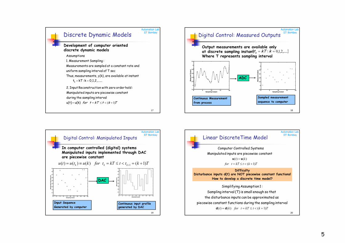
Discrete Dynamic Models
17
..0,1,2,....k:kTt
instant at available are (k), ts,measuremen Thus,
sec T of interval sampling uniform
and rate constant a at sampled are tsMeasuremen
:Sampling tMeasuremen 1.
sAssumption
k
y
TktkTtfor )1( u(k)u(t)
interval sampling the during
constant piecewise are inputs dManipulate
:hold order zero with tionReconstruc Input 2.
Development of computer oriented discrete dynamic models
Automation LabIIT Bombay
18
Digital Control: Measured Outputs
0 5 10 15 201.8
2
2.2
2.4
2.6
2.8
3
3.2
Sampling Instant
Measu
red
Ou
tpu
t
0 5 10 15 201.8
2
2.2
2.4
2.6
2.8
3
3.2
Sampling Instant
Measu
red
Ou
tpu
t
ADC
Continuous Measurement
from process
Sampled measurement
sequence to computer
Output measurements are available onlyat discrete sampling instant Where T represents sampling interval
,....,,: 210 kkTtk
Automation LabIIT Bombay
19
Digital Control: Manipulated Inputs
In computer controlled (digital) systems Manipulated inputs implemented through DACare piecewise constant
0 2 4 6 8 10 12 14 16 18 202
2.1
2.2
2.3
2.4
2.5
2.6
2.7
2.8
2.9
Sampling Instant
Man
ipu
late
d In
pu
t
0 2 4 6 8 10 12 14 16 18 202
2.1
2.2
2.3
2.4
2.5
2.6
2.7
2.8
2.9
Sampling Instant
Ma
nip
ula
ted
In
pu
t S
eq
uen
ce
DAC
Input Sequence
Generated by computerContinuous input profile generated by DAC
TkttkTtforkututu kkk )1()()()( 1
Automation LabIIT Bombay
20
Linear DiscreteTime Model
TktkTtfor
kt
)1(
)()(
uu
constant piecewise are inputs dManipulate
Systems Controlled Computer
DifficultyDisturbance inputs d(t) are NOT piecewise constant functions!
How to develop a discrete time model?
TktkTtforkt )1()()( dd
interval sampling the during functions constant piecewise
as edapproximat be can inputs edisturbanc the
that so enough small is (T) interval Sampling
:1 Assumption gSimplifyin
6
Automation LabIIT Bombay
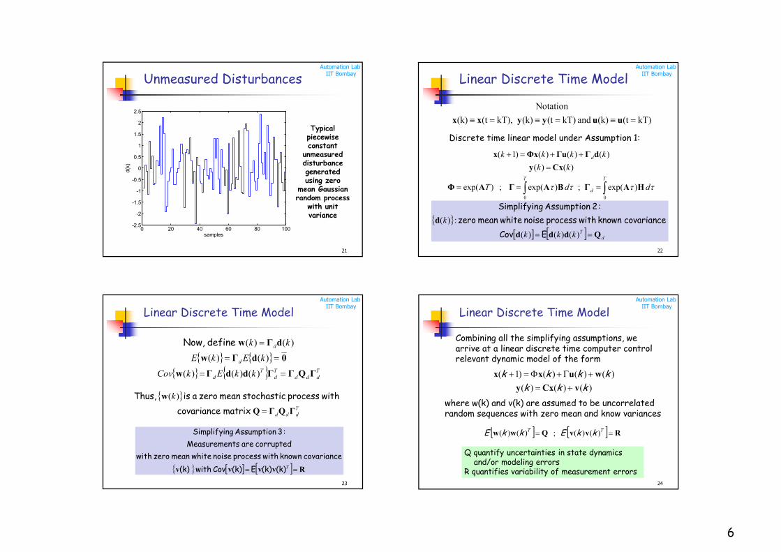
Unmeasured Disturbances
21
0 20 40 60 80 100-2.5
-2
-1.5
-1
-0.5
0
0.5
1
1.5
2
2.5
samples
d(k
)Typical
piecewise constant
unmeasured disturbance generated using zero
mean Gaussian random process
with unit variance
Automation LabIIT Bombay
22
Linear Discrete Time Model
Discrete time linear model under Assumption 1:
ddT
kk
kkkk
T
d
T
d
HAΓBAΓAΦ
Cxy
dΓΓuΦxx
)exp(;)exp(;)exp(
)()(
)()()()1(
00
dTkkk
k
Qddd
d
)()()(
:)(
ECov
covariance known with process noise white mean zero
:2 Assumption gSimplifyin
kT)(t(k) and kT)(t(k)kT),(t(k)
Notation
uuyyxx
Automation LabIIT Bombay
23
Linear Discrete Time Model
Rvvvv T(k)(k)E(k)Cov with (k)
covariance known with process noise white mean zero with
corrupted are tsMeasuremen
:3 Assumption gSimplifyin
T
dddTd
Td
d
d
kkEkCov
kEkE
kk
ΓQΓΓddΓw
0dΓw
dΓw
)()()(
)()(
)()( define Now,
Tddd
k
ΓQΓQ
w
matrix covariance
with process stochastic mean zero a is Thus, )(
Automation LabIIT Bombay
24
Linear Discrete Time Model
)()()(
)()()()1(
kkk
kkkk
vCxy
wuxx
Combining all the simplifying assumptions, we arrive at a linear discrete time computer controlrelevant dynamic model of the form
where w(k) and v(k) are assumed to be uncorrelated random sequences with zero mean and know variances
RvvQww TT kkEkkE )()(;)()(
Q quantify uncertainties in state dynamicsand/or modeling errors
R quantifies variability of measurement errors
7
Automation LabIIT Bombay
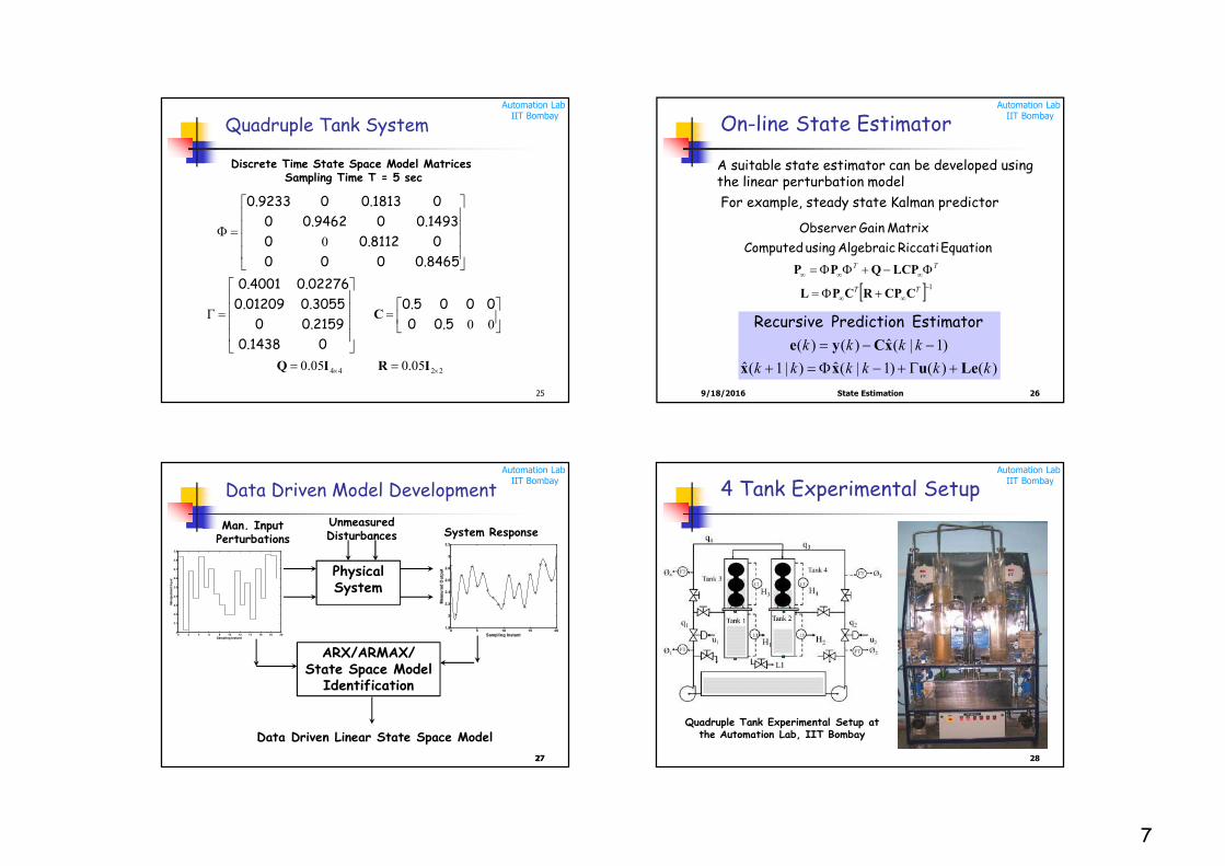
Quadruple Tank System
25
2244 05.005.0
00
0
IRIQ
C 0.50
0000.5
00.1438
0.21590
0.30550.01209
0.022760.4001
0.8465000
0 0.81120
0.149300.94620
00.181300.9233
Discrete Time State Space Model Matrices Sampling Time T = 5 sec
Automation LabIIT Bombay
9/18/2016 State Estimation 26
On-line State Estimator
)()()1|(ˆ)|1(ˆ
)1|(ˆ)()(
kkkkkk
kkkk
Leuxx
xCye
Estimator Prediction Recursive
1
TT
TT
CCPRCPL
LCPQPP
Equation Riccati Algebraic using Computed
Matrix Gain Observer
For example, steady state Kalman predictor
A suitable state estimator can be developed using the linear perturbation model
Automation LabIIT Bombay
Data Driven Model Development
2727
0 2 4 6 8 10 12 14 16 18 202
2.1
2.2
2.3
2.4
2.5
2.6
2.7
2.8
2.9
Sampling Instant
Man
ipu
late
d In
pu
t
Physical System
0 5 10 15 201.8
2
2.2
2.4
2.6
2.8
3
3.2
Sampling Instant
Measu
red
Ou
tpu
t
Man. Input Perturbations
System ResponseUnmeasured Disturbances
ARX/ARMAX/ State Space Model
Identification
Data Driven Linear State Space Model
Automation LabIIT Bombay
4 Tank Experimental Setup
28
Quadruple Tank Experimental Setup at the Automation Lab, IIT Bombay
8
Automation LabIIT Bombay
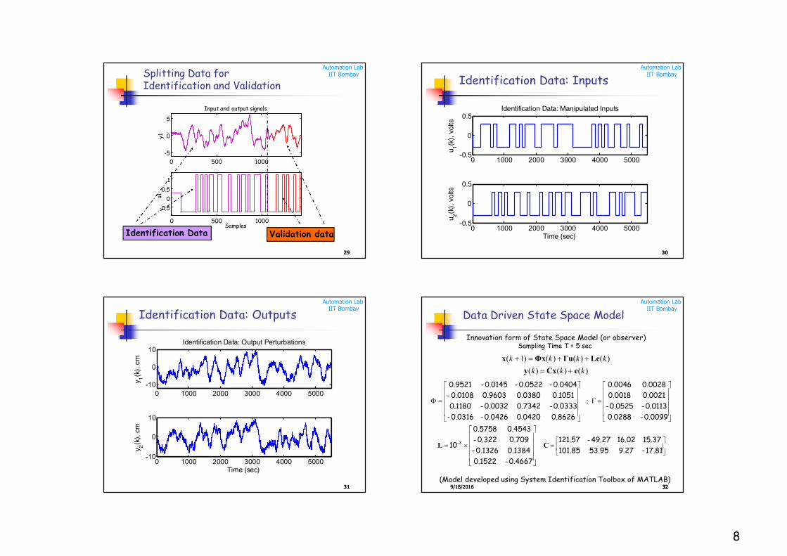
29
Splitting Data for Identification and Validation
0 500 1000
-5
0
5
y1
Input and output signals
0 500 1000
-0.5
0
0.5
1
Samples
u1
Identification Data Validation data
Automation LabIIT Bombay
30
Identification Data: Inputs
0 1000 2000 3000 4000 5000-0.5
0
0.5
u1(k
), v
olts
Identification Data: Manipulated Inputs
0 1000 2000 3000 4000 5000-0.5
0
0.5
Time (sec)
u2(k
), v
olts
Automation LabIIT Bombay
31
Identification Data: Outputs
0 1000 2000 3000 4000 5000
-10
0
10
y 1(k
), c
m
Identification Data: Output Perturbations
0 1000 2000 3000 4000 5000-10
0
10
Time (sec)
y 2(k
), c
m
Automation LabIIT Bombay
32329/18/2016 32
Data Driven State Space Model
9/18/2016 32
17.81-9.2753.95101.85
15.3716.0249.27-121.57
0.4667-0.1522
0.13840.1326-
0.7090.322-
0.45430.5758
10
0.0099-0.0288
0.0113-0.0525-
0.00210.0018
0.00280.0046
0.86260.04200.0426-0.0316-
0.0333-0.73420.0032-0.1180
0.10510.03800.96030.0108-
0.0404-0.0522-0.0145-0.9521
3-
CL
;
Innovation form of State Space Model (or observer)Sampling Time T = 5 sec
)()()(
)()()()1(
kkk
kkkk
eCxy
LeΓuΦxx
(Model developed using System Identification Toolbox of MATLAB)
9
Automation LabIIT Bombay
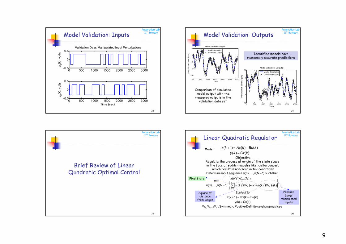
Model Validation: Inputs
33
0 500 1000 1500 2000 2500 3000-0.5
0
0.5
u1(k
), v
olts
Validation Data: Manipulated Input Perturbations
0 500 1000 1500 2000 2500 3000-0.5
0
0.5
Time (sec)
u2(k
), v
olts
Automation LabIIT Bombay
Model Validation: Outputs
34
0 500 1000 1500 2000 2500 3000
-10
-5
0
5
10
Time
Pe
rturb
atio
n L
eve
l 1 (
cm)
Model Validation: Output 1
Model Simulation
Measured Output
0 500 1000 1500 2000 2500 3000-10
-5
0
5
10
Time
Pe
rtu
rba
tion
Le
vel 2
(cm
)
Model Validation: Output 2
Model Simulation
Measured Output
Identified models have reasonably accurate predictions
Comparison of simulated model output with the
measured outputs in the validation data set
Automation LabIIT Bombay
35
Brief Review of Linear Quadratic Optimal Control
Automation LabIIT Bombay
3636
Linear Quadratic Regulator
)()(
)()()1(
kCxky
kBukAxkx
Model:
ObjectiveRegulate the process at origin of the state space in the face of sudden impulse like, disturbances,
which result in non-zero initial conditions
matrices seighting Definite PositiveSymmetric :W,WW
Cx(k)y(k)
)(x(k)1)x(k
u(k)Wu(k))()(
)()(
)1(),....,0(
min
that such)1(),....,0( sequence input Determine
N x,
1
0u
T
u
N
kx
T
NT
ku
toSubject
kxWkx
NxWNx
Nuu
Nuu
Square of distance
from Origin
PenalizeLarge
manipulated inputs
Final State
10
Automation LabIIT Bombay
3737
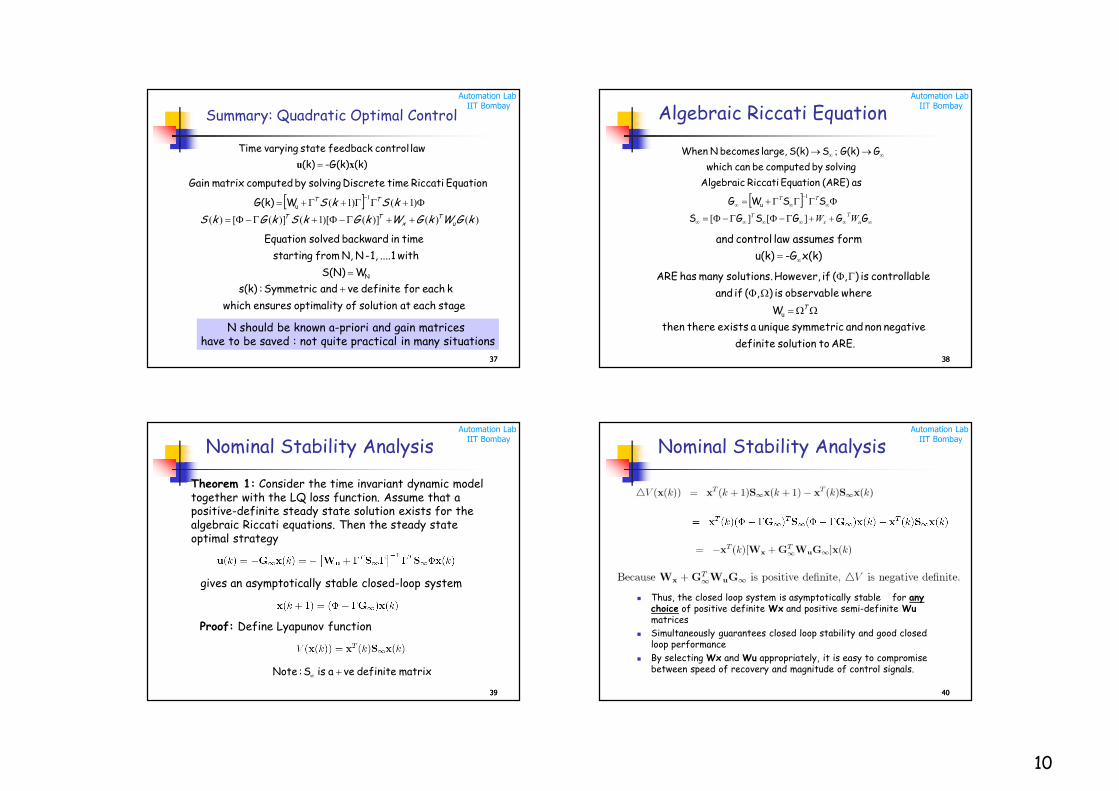
Summary: Quadratic Optimal Control
(k)-G(k)(k)
law control feedback state varying Time
xu
stage each at solution of optimality ensures which
k each for definite ve and Symmetric : s(k)
WS(N)
with ....1 1,-N N, from starting
time in backward solved Equation
N
)()()]()[1()]([)(
)1()1(1
kGWkGWkGkSkGkS
kSkS
uT
xTT
TT
uWG(k)
Equation Riccati time Discrete solving by computed matrix Gain
N should be known a-priori and gain matrices have to be saved : not quite practical in many situations
Automation LabIIT Bombay
3838
Algebraic Riccati Equation
GGGSGS
SSWG
as (ARE) Equation Riccati Algebraic
solving by computed be can which
GG(k)SS(k) large, becomes N When
u
u
T
xT
TT
WW][][
;
1
ARE. to solution definite
negative non and symmetric unique a exists there then
W
where observable is ),( if and
lecontrollab is ),( if However, solutions. many has ARE
u
T
x(k)-Gu(k)
form assumes law control and
Automation LabIIT Bombay
3939
Nominal Stability Analysis
Theorem 1: Consider the time invariant dynamic model together with the LQ loss function. Assume that a positive-definite steady state solution exists for the algebraic Riccati equations. Then the steady state optimal strategy
gives an asymptotically stable closed-loop system
Proof: Define Lyapunov function
matrix definite ve a is S :Note
Automation LabIIT Bombay
4040
Nominal Stability Analysis
Thus, the closed loop system is asymptotically stable for any choice of positive definite Wx and positive semi-definite Wumatrices
Simultaneously guarantees closed loop stability and good closed loop performance
By selecting Wx and Wu appropriately, it is easy to compromise between speed of recovery and magnitude of control signals.
11
Automation LabIIT Bombay
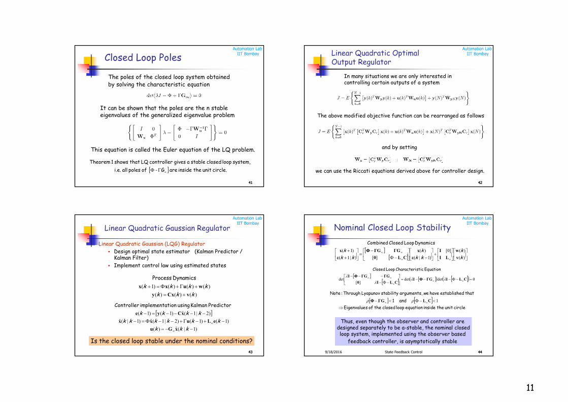
4141
Closed Loop Poles
The poles of the closed loop system obtained
by solving the characteristic equation
It can be shown that the poles are the n stable eigenvalues of the generalized eigenvalue problem
This equation is called the Euler equation of the LQ problem.
circle. unit the inside are G- of poles all i.e.
system, loop closed stable a gives controller LQ that shows 1 Theorem
Automation LabIIT Bombay
4242
Linear Quadratic Optimal Output Regulator
In many situations we are only interested in controlling certain outputs of a system
The above modified objective function can be rearranged as follows
and by setting
we can use the Riccati equations derived above for controller design.
Automation LabIIT Bombay
4343
Linear Quadratic Gaussian Regulator
Linear Quadratic Gaussian (LQG) Regulator
Design optimal state estimator (Kalman Predictor / Kalman Filter)
Implement control law using estimated states
)()()(
)()()()1(
kkk
kkkk
vCxy
wuxx
Dynamics Process
)1|(ˆ)(
)1()1()2|1(ˆ)1|(ˆ
)2|1(ˆ)1()1(
kkk
kkkkkk
kkkk
xGu
eLuxx
xCye
Predictor Kalman using tionimplementa Controller
Is the closed loop stable under the nominal conditions?
Automation LabIIT Bombay
449/18/2016 State Feedback Control 44
Nominal Closed Loop Stability
)(
)(]0[
)1|(
)(
][)|1(
)1(
k
k
kk
k
kk
k
v
w
LI
I
ε
x
CL0
ΓGΓGΦ
ε
x
Dynamics Loop Closed Combined
circle unit the inside equation loop closed the of sEigenvalue
and 1
that destablishe have e arguments, stability Lyapunov Through :Note
1CLΓGΦ
w
0detdet
][det
CLIΓGΦICLI0
ΓGΓGΦI
Equation sticCharacteri Loop Closed
Thus, even though the observer and controller are designed separately to be a-stable, the nominal closedloop system, implemented using the observer based
feedback controller, is asymptotically stable
12
Automation LabIIT Bombay
4545
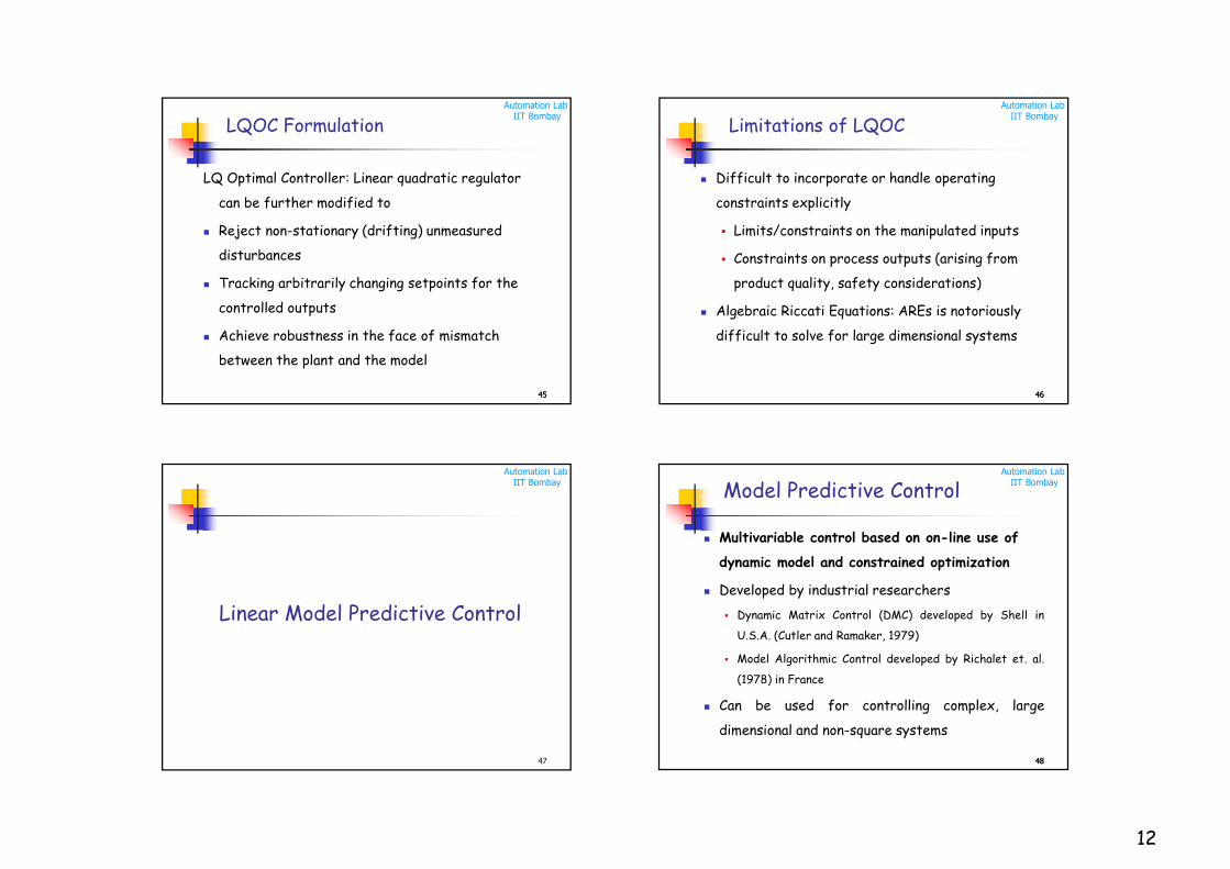
LQOC Formulation
LQ Optimal Controller: Linear quadratic regulator
can be further modified to
Reject non-stationary (drifting) unmeasured
disturbances
Tracking arbitrarily changing setpoints for the
controlled outputs
Achieve robustness in the face of mismatch
between the plant and the model
Automation LabIIT Bombay
4646
Limitations of LQOC
Difficult to incorporate or handle operating
constraints explicitly
Limits/constraints on the manipulated inputs
Constraints on process outputs (arising from
product quality, safety considerations)
Algebraic Riccati Equations: AREs is notoriously
difficult to solve for large dimensional systems
Automation LabIIT Bombay
47
Linear Model Predictive Control
Automation LabIIT Bombay
4848
Model Predictive Control
Multivariable control based on on-line use of
dynamic model and constrained optimization
Developed by industrial researchers
Dynamic Matrix Control (DMC) developed by Shell in
U.S.A. (Cutler and Ramaker, 1979)
Model Algorithmic Control developed by Richalet et. al.
(1978) in France
Can be used for controlling complex, large
dimensional and non-square systems
13
Automation LabIIT Bombay
4949
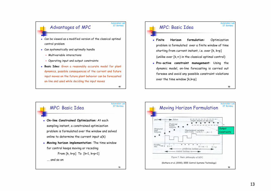
Advantages of MPC
Can be viewed as a modified version of the classical optimal
control problem
Can systematically and optimally handle
Multivariable interactions
Operating input and output constraints
Basic Idea: Given a reasonably accurate model for plant
dynamics, possible consequences of the current and future
input moves on the future plant behavior can be forecasted
on-line and used while deciding the input moves
Automation LabIIT Bombay
5050
MPC: Basic Idea
Finite Horizon formulation: Optimization
problem is formulated over a finite window of time
starting from current instant, i.e. over [k, k+p]
(unlike over [k,∞) in the classical optimal control)
Pro-active constraint management: Using the
dynamic model, on-line forecasting is carried out
foresee and avoid any possible constraint violations
over the time window [k,k+p]
Automation LabIIT Bombay
5151
MPC: Basic Idea
On-line Constrained Optimization: At each
sampling instant, a constrained optimization
problem is formulated over the window and solved
online to determine the current input u(k)
Moving horizon implementation: The time window
for control keeps moving or receding
From [k, k+p] To [k+1, k+p+1]
…. and so on
Automation LabIIT Bombay
5252
Moving Horizon Formulation
(Kothare et al, (2000), IEEE Control Systems Technology)
Output
Constraints
14
Automation LabIIT Bombay
5353
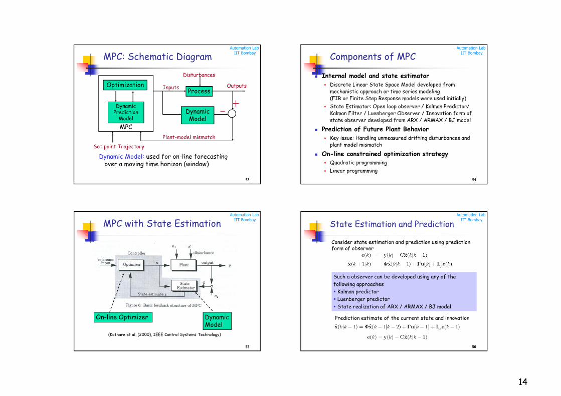
MPC: Schematic Diagram
Process
Dynamic Model
Dynamic Prediction
Model
Optimization
MPC
Set point Trajectory
Disturbances
Dynamic Model: used for on-line forecasting over a moving time horizon (window)
Plant-model mismatch
Inputs Outputs
Automation LabIIT Bombay
5454
Components of MPC
Internal model and state estimator
Discrete Linear State Space Model developed from
mechanistic approach or time series modeling
(FIR or Finite Step Response models were used initially)
State Estimator: Open loop observer / Kalman Predictor/
Kalman Filter / Luenberger Observer / Innovation form of
state observer developed from ARX / ARMAX / BJ model
Prediction of Future Plant Behavior
Key issue: Handling unmeasured drifting disturbances and
plant model mismatch
On-line constrained optimization strategy
Quadratic programming
Linear programming
Automation LabIIT Bombay
5555
MPC with State Estimation
DynamicModel
(Kothare et al, (2000), IEEE Control Systems Technology)
On-line Optimizer
Automation LabIIT Bombay
5656
State Estimation and Prediction
Consider state estimation and prediction using prediction form of observer
Such a observer can be developed using any of the
following approaches
Kalman predictor
Luenberger predictor
State realization of ARX / ARMAX / BJ model
Prediction estimate of the current state and innovation
15
Automation LabIIT Bombay
5757
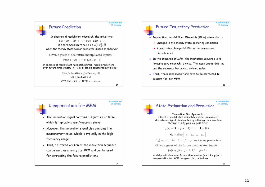
Future Prediction
in absence of model plant mismatch (MPM), model predictions over future time window [k + 1; k+p] can be generated as follows
observer as used is predictor Kalman state steady the when
i.e. noise, white mean zero a is
sinnivation the mismatch, plant model of absence In
0e
xCyyye
)(
)1|(ˆ)()1|(ˆ)()(
kE
kkkkkkk
pjkkk
jkjk
kjkjkjk
,...,2,1)1|(ˆ)(ˆ
)(ˆ)(ˆ
)|()(ˆ)1(ˆ
for with xz
zCy
ΓuzΦz
Automation LabIIT Bombay
Future Trajectory Prediction
In practice, Model Plant Mismatch (MPM) arises due to
Changes in the steady state operating conditions
Abrupt step changes/drifts in the unmeasured
disturbances
In the presence of MPM, the innovation sequence is no
longer a zero mean white noise. The mean starts drifting
and the sequence becomes a colored noise.
Thus, the model predictions have to be corrected to
account for for MPM
5858
Automation LabIIT Bombay
Compensation for MPM
The innovation signal contains a signature of MPM,
which is typically a low frequency signal
However, the innovation signal also contains the
measurement noise, which is typically in the high
frequency range
Thus, a filtered version of the innovation sequence
can be used as a proxy for MPM and can be used
for correcting the future predictions
59
Automation LabIIT Bombay
6060
State Estimation and Prediction
Innovation Bias Approach: Effect of model plant mismatch and /or unmeasured
disturbance signal is extracted by filtering the innovationthrough a unity gain low pass filter
model predictions over future time window [k + 1; k + p] with compensation for MPM are generated as follows
16
Automation LabIIT Bombay
6161
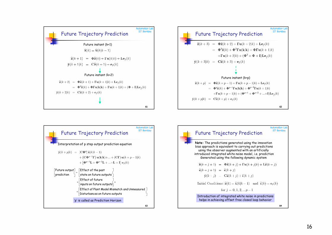
Future Trajectory Prediction
Future instant (k+2)
Future instant (k+1)
Automation LabIIT Bombay
6262
Future Trajectory Prediction
Future instant (k+p)
Automation LabIIT Bombay
6363
Future Trajectory Prediction
outputs future on esDisturbanc
Unmeasured and Mismatch Model Plant of Effect
outputs future on inputs
future of Effect
outputs future on state
past the of Effect
prediction
output Future
Interpretation of p step output prediction equation
‘p’ is called as Prediction Horizon
Automation LabIIT Bombay
6464
Future Trajectory Prediction
Note: The predictions generated using the innovation bias approach is equivalent to carrying out predictions
using the observer augmented with an artificially introduced integrated white noise model, i.e. prediction
Generated using the following dynamic system
Introduction of integrated white noise in predictionshelps in achieving offset free closed loop behavior
17
Automation LabIIT Bombay
6565
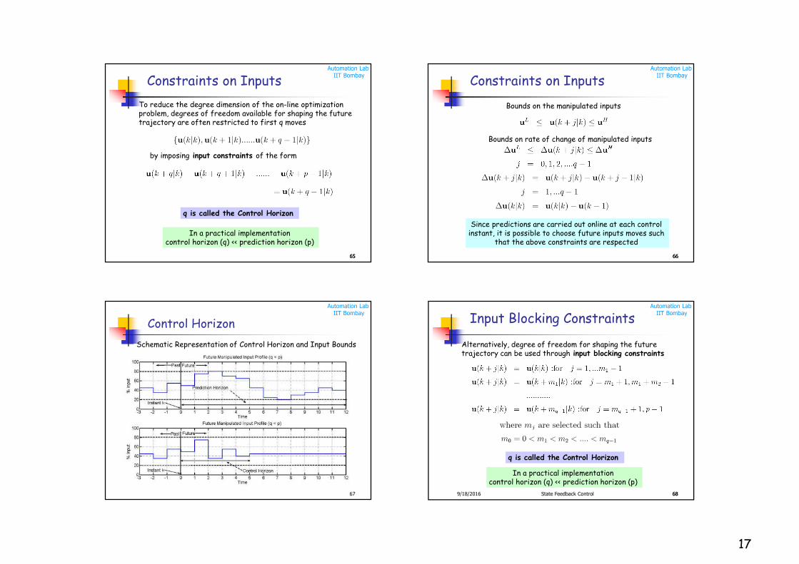
Constraints on Inputs
q is called the Control Horizon
In a practical implementation control horizon (q) << prediction horizon (p)
To reduce the degree dimension of the on-line optimization problem, degrees of freedom available for shaping the future trajectory are often restricted to first q moves
by imposing input constraints of the form
Automation LabIIT Bombay
6666
Constraints on Inputs
Since predictions are carried out online at each control instant, it is possible to choose future inputs moves such
that the above constraints are respected
Bounds on rate of change of manipulated inputs
Bounds on the manipulated inputs
Automation LabIIT Bombay
67
Control Horizon
Schematic Representation of Control Horizon and Input Bounds
Automation LabIIT Bombay
689/18/2016 State Feedback Control 68
Input Blocking Constraints
Alternatively, degree of freedom for shaping the future trajectory can be used through input blocking constraints
q is called the Control Horizon
In a practical implementation control horizon (q) << prediction horizon (p)
18
Automation LabIIT Bombay
699/18/2016 State Feedback Control 69
Input Blocking Constraints
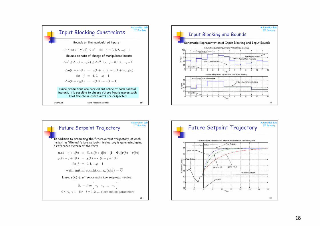
Bounds on the manipulated inputs
Bounds on rate of change of manipulated inputs
Since predictions are carried out online at each control instant, it is possible to choose future inputs moves such
That the above constraints are respected
Automation LabIIT Bombay
70
Input Blocking and Bounds
Schematic Representation of Input Blocking and Input Bounds
Automation LabIIT Bombay
7171
Future Setpoint Trajectory
In addition to predicting the future output trajectory, at each instant, a filtered future setpoint trajectory is generated using a reference system of the form
Automation LabIIT Bombay
72
Future Setpoint Trajectory
19
Automation LabIIT Bombay
739/18/2016 State Feedback Control 73
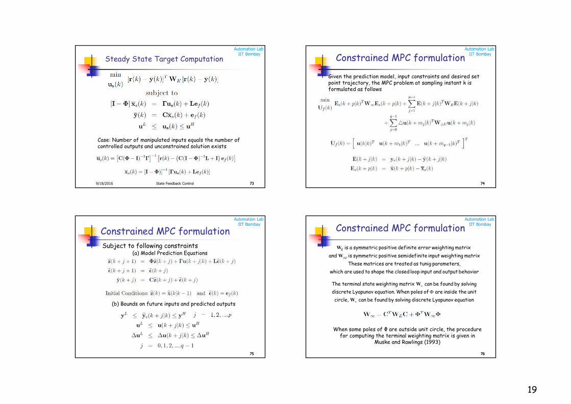
Steady State Target Computation
Case: Number of manipulated inputs equals the number of controlled outputs and unconstrained solution exists
Automation LabIIT Bombay
74
Constrained MPC formulation
74
Given the prediction model, input constraints and desired set point trajectory, the MPC problem at sampling instant k is formulated as follows
Automation LabIIT Bombay
75
Constrained MPC formulation
75
Subject to following constraints(a) Model Prediction Equations
(b) Bounds on future inputs and predicted outputs
Automation LabIIT Bombay
76
Constrained MPC formulation
76
behavior output and input loop closed the shape to used are which
,parameters tunig as treated are matrices These
matrix weighting input tesemidefini positive symmetric is and
matrix weighting error definite positive symmetric a is
U
E
W
W
equation Lyapunov discrete solving by found be can circle,
unit the inside are of poles When equation. Lyapunov discrete
solving by found be can matrix weighting state terminal The
W
W
When some poles of Φ are outside unit circle, the procedure for computing the terminal weighting matrix is given in
Muske and Rawlings (1993)
20
Automation LabIIT Bombay
77
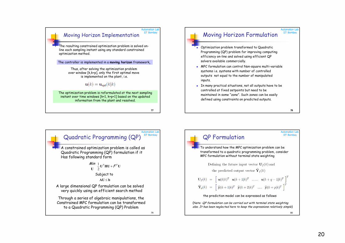
Moving Horizon Implementation
77
The resulting constrained optimization problem is solved on-line each sampling instant using any standard constrained optimization method.
The controller is implemented in a moving horizon framework.
Thus, after solving the optimization problem over window [k,k+p], only the first optimal move
is implemented on the plant, i.e.
The optimization problem is reformulated at the next sampling instant over time windows [k+1, k+p+1] based on the updated
information from the plant and resolved.
Automation LabIIT Bombay
7878
Moving Horizon Formulation
Optimization problem transformed to Quadratic
Programming (QP) problem for improving computing
efficiency on-line and solved using efficient QP
solvers available commercially.
MPC formulation can control Non-square multi-variable
systems i.e. systems with number of controlled
outputs not equal to the number of manipulated
inputs.
In many practical situations, not all outputs have to be
controlled at fixed setpoints but need to be
maintained in some “zone”. Such zones can be easily
defined using constraints on predicted outputs.
Automation LabIIT Bombay
79
Quadratic Programming (QP)
A constrained optimization problem is called as Quadratic Programming (QP) formulation if it Has following standard form
bAU
UHUUU
to Subject
TT FMin
2
1
A large dimensional QP formulation can be solved very quickly using an efficient search method
Through a series of algebraic manipulations, the Constrained MPC formulation can be transformed
to a Quadratic Programming (QP) Problem
Automation LabIIT Bombay
80
QP Formulation
To understand how the MPC optimization problem can be
transformed to a quadratic programming problem, considerMPC formulation without terminal state weighting
(Note: QP formulation can be carried out with terminal state weighting
also. It has been neglected here to keep the expressions relatively simple)
the prediction model can be expressed as follows
21
Automation LabIIT Bombay
81
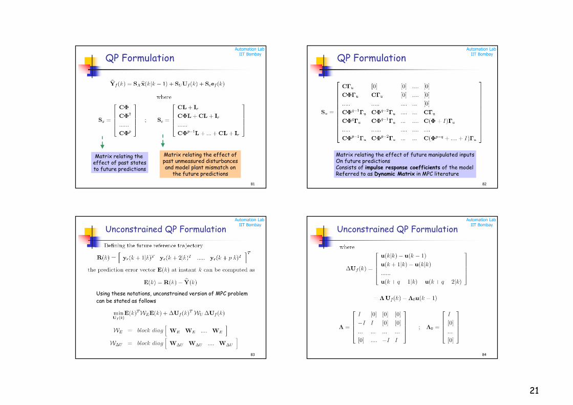
QP Formulation
Matrix relating the effect of past statesto future predictions
Matrix relating the effect ofpast unmeasured disturbancesand model plant mismatch on
the future predictions
Automation LabIIT Bombay
82
QP Formulation
Matrix relating the effect of future manipulated inputsOn future predictionsConsists of impulse response coefficients of the modelReferred to as Dynamic Matrix in MPC literature
Automation LabIIT Bombay
83
Unconstrained QP Formulation
Using these notations, unconstrained version of MPC problem
can be stated as follows
Automation LabIIT Bombay
84
Unconstrained QP Formulation
22
Automation LabIIT Bombay
85
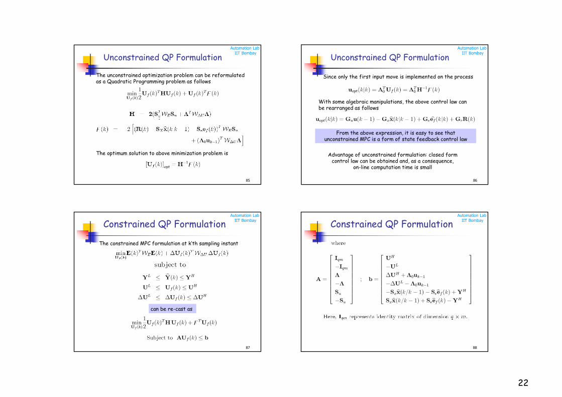
Unconstrained QP Formulation
The unconstrained optimization problem can be reformulated as a Quadratic Programming problem as follows
The optimum solution to above minimization problem is
Automation LabIIT Bombay
86
Unconstrained QP Formulation
Since only the first input move is implemented on the process
With some algebraic manipulations, the above control law can be rearranged as follows
From the above expression, it is easy to see that unconstrained MPC is a form of state feedback control law
Advantage of unconstrained formulation: closed form control law can be obtained and, as a consequence,
on-line computation time is small
Automation LabIIT Bombay
87
Constrained QP Formulation
The constrained MPC formulation at k’th sampling instant
can be re-cast as
Automation LabIIT Bombay
88
Constrained QP Formulation
23
Automation LabIIT Bombay
89
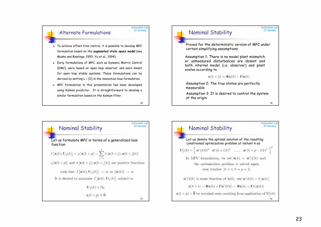
Alternate Formulations
To achieve offset free control, it is possible to develop MPC
formulation based on the augmented state space model (see
Muske and Rawlings, 1993; Yu et al., 1994).
Early formulations of MPC, such as Dynamic Matrix Control
(DMC), were based on ‘open loop observer’ and were meant
for open loop stable systems. These formulations can be
derived by setting L = [0] in the innovation bias formulation.
MPC formulation in this presentation has been developed
using Kalman predictor. It is straightforward to develop a
similar formulation based on the Kalman filter.
Automation LabIIT Bombay
Nominal Stability
90
Proved for the deterministic version of MPC undercertain simplifying assumptions
Assumption 2: The true states are perfectly measurable
Assumption 3: It is desired to control the system at the origin
Assumption 1: There is no model plant mismatchor unmeasured disturbances are absent andboth internal model (i.e. observer) and plantevolve according to
Automation LabIIT Bombay
Nominal Stability
91
Let us formulate MPC in terms of a generalized loss function
Automation LabIIT Bombay
Nominal Stability
92
Let us denote the optimal solution of the resulting constrained optimization problem at instant k as
24
Automation LabIIT Bombay
Nominal Stability
93
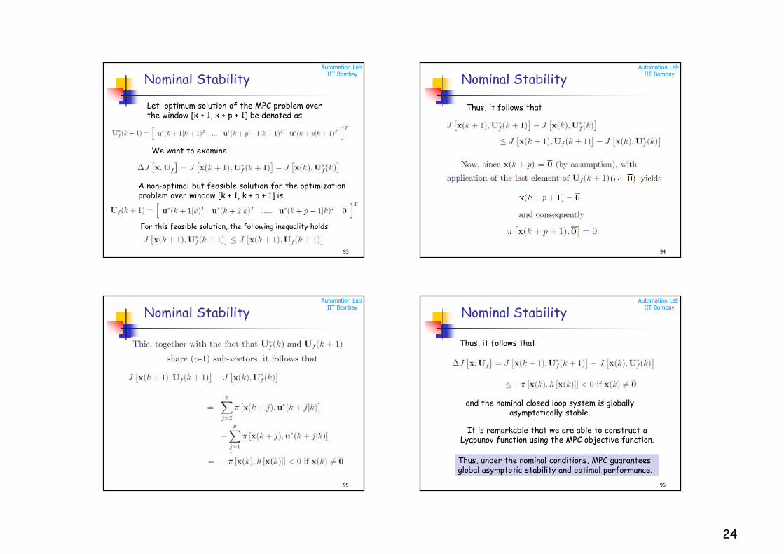
Let optimum solution of the MPC problem over the window [k + 1, k + p + 1] be denoted as
We want to examine
A non-optimal but feasible solution for the optimization problem over window [k + 1, k + p + 1] is
For this feasible solution, the following inequality holds
Automation LabIIT Bombay
Nominal Stability
94
Thus, it follows that
Automation LabIIT Bombay
Nominal Stability
95
Automation LabIIT Bombay
Nominal Stability
96
Thus, it follows that
and the nominal closed loop system is globally asymptotically stable.
Thus, under the nominal conditions, MPC guarantees global asymptotic stability and optimal performance.
It is remarkable that we are able to construct a Lyapunov function using the MPC objective function.
25
Automation LabIIT Bombay
97
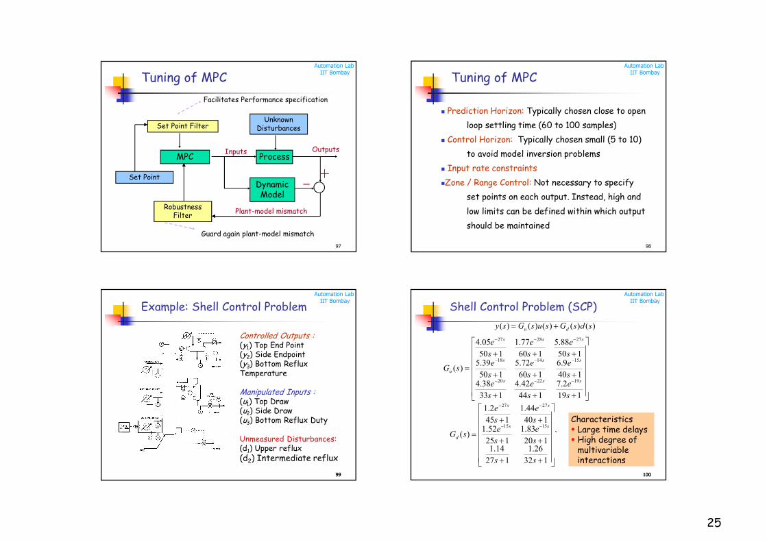
Tuning of MPC
Process
Dynamic Model
Unknown DisturbancesSet Point Filter
MPC
Plant-model mismatch
Inputs Outputs
Robustness Filter
Set Point
Facilitates Performance specification
Guard again plant-model mismatch
Automation LabIIT Bombay
98
Tuning of MPC
Prediction Horizon: Typically chosen close to open
loop settling time (60 to 100 samples)
Control Horizon: Typically chosen small (5 to 10)
to avoid model inversion problems
Input rate constraints
Zone / Range Control: Not necessary to specify
set points on each output. Instead, high and
low limits can be defined within which output
should be maintained
Automation LabIIT Bombay
9999
Example: Shell Control Problem
Controlled Outputs :(y1) Top End Point (y2) Side Endpoint (y3) Bottom Reflux Temperature
Manipulated Inputs :(u1) Top Draw (u2) Side Draw (u3) Bottom Reflux Duty
Unmeasured Disturbances:(d1) Upper reflux
(d2) Intermediate reflux
Automation LabIIT Bombay
100100
119
2.7
144
42.4
133
38.4140
9.6
160
72.5
150
39.5150
88.5
160
77.1
150
05.4
)(
192220
151418
272827
s
e
s
e
s
es
e
s
e
s
es
e
s
e
s
e
sG
sss
sss
sss
u
)()()()()( sdsGsusGsy du
`
132
26.1
127
14.1120
83.1
125
52.1140
44.1
145
2.1
)(1515
2727
ss
s
e
s
es
e
s
e
sGss
ss
d
Characteristics Large time delays High degree of
multivariable interactions
Shell Control Problem (SCP)
26
Automation LabIIT Bombay
101101
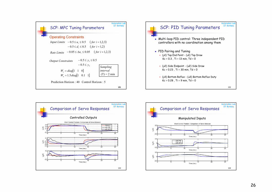
SCP: MPC Tuning Parameters
Operating Constraints
3
1
5.0
5.05.0
y
y
Input Limits
2,15.05.0
3,2,15.05.0
iford
iforu
i
i
3,2,105.005.0 iforuiRate Limits
Output Constraints
Prediction Horizon : 40 Control Horizon : 5
11.015.1
011
diagW
diagW
u
e
Sampling interval(T) = 2 min
Automation LabIIT Bombay
102
SCP: PID Tuning Parameters
Multi-loop PID control: Three independent PID controllers with no coordination among them
PID Pairing and Tuning (y1) Top End Point - (u1) Top Draw
Kc = 0.3 , Ti = 13 min, Td = 0
(y2) Side Endpoint - (u2) Side Draw
Kc = 0.23 , Ti = 30 min, Td = 0
(y3) Bottom Reflux - (u3) Bottom Reflux Duty
Kc = 0.28 , Ti = 9 min, Td = 0
Automation LabIIT Bombay
103
Comparison of Servo Responses
Controlled Outputs
Automation LabIIT Bombay
104
Comparison of Servo Responses
Manipulated Inputs
27
Automation LabIIT Bombay
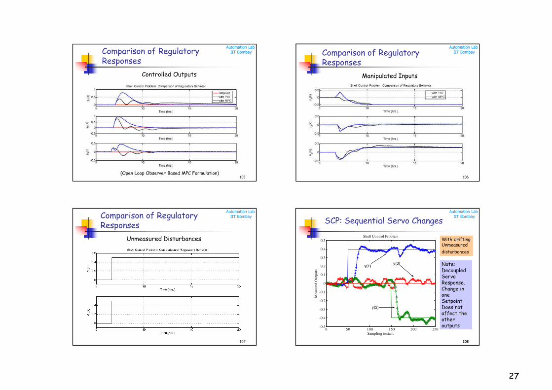
105
Comparison of Regulatory Responses
Controlled Outputs
(Open Loop Observer Based MPC Formulation)
Automation LabIIT Bombay
106
Comparison of Regulatory Responses
Manipulated Inputs
Automation LabIIT Bombay
107
Comparison of Regulatory Responses
Unmeasured Disturbances
Automation LabIIT Bombay
108108
SCP: Sequential Servo Changes
0 50 100 150 200 250-0.5
-0.4
-0.3
-0.2
-0.1
0
0.1
0.2
0.3
0.4
0.5
Sampling instant
Mea
sure
d O
utp
uts
Shell Control Problem
y(1)
y(2)
y(3) Note:DecoupledServoResponse. Change in oneSetpoint Does not affect the other outputs
With driftingUnmeasured
disturbances
28
Automation LabIIT Bombay
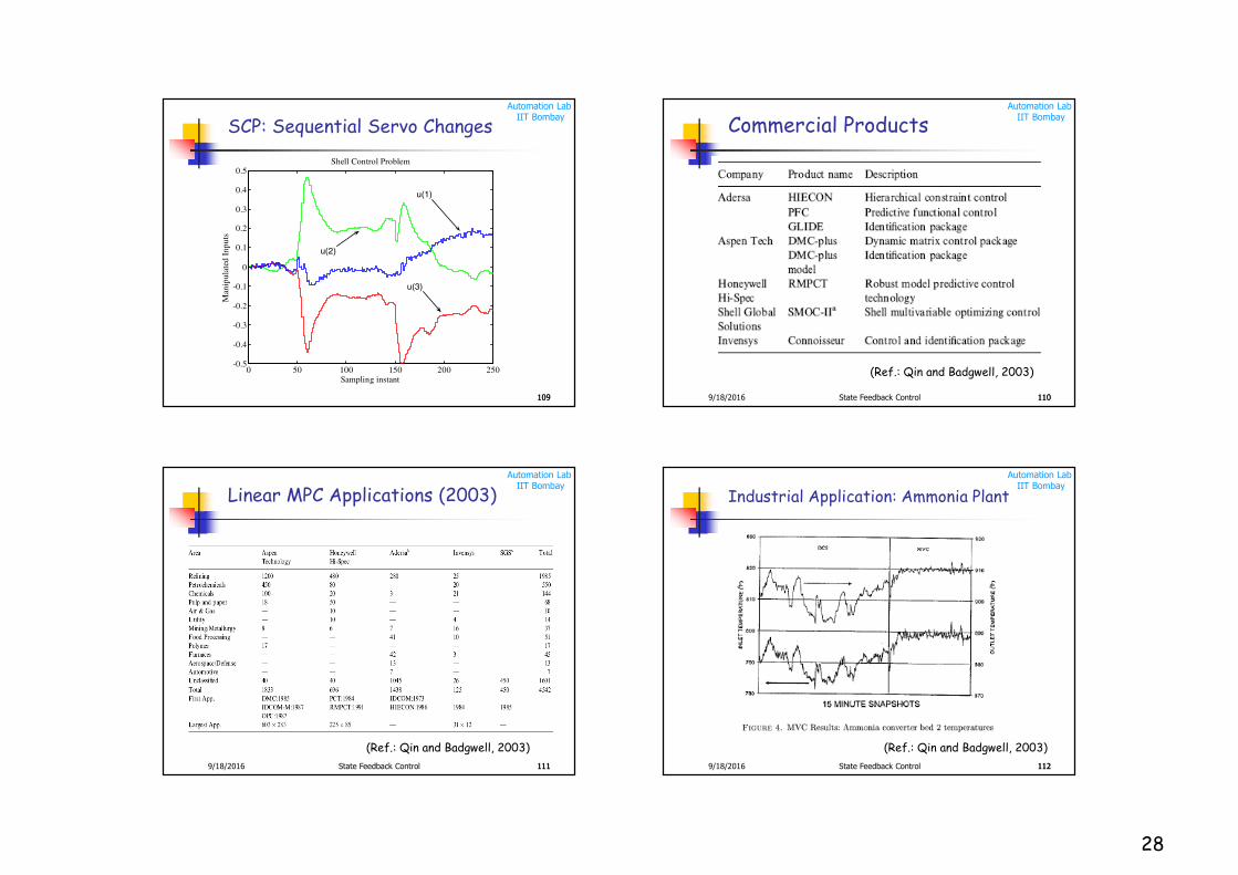
109109
SCP: Sequential Servo Changes
0 50 100 150 200 250-0.5
-0.4
-0.3
-0.2
-0.1
0
0.1
0.2
0.3
0.4
0.5
Sampling instant
Man
ipu
late
d I
np
uts
Shell Control Problem
u(1)
u(2)
u(3)
Automation LabIIT Bombay
1109/18/2016 State Feedback Control 110
Commercial Products
(Ref.: Qin and Badgwell, 2003)
Automation LabIIT Bombay
1119/18/2016 State Feedback Control 111
Linear MPC Applications (2003)
(Ref.: Qin and Badgwell, 2003)
Automation LabIIT Bombay
1129/18/2016 State Feedback Control 112
Industrial Application: Ammonia Plant
(Ref.: Qin and Badgwell, 2003)
29
Automation LabIIT Bombay
113
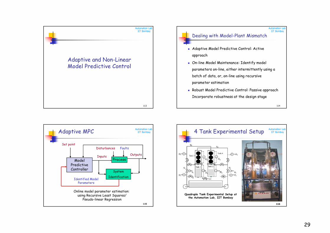
Adaptive and Non-Linear Model Predictive Control
Automation LabIIT Bombay
Dealing with Model-Plant Mismatch
Adaptive Model Predictive Control: Active
approach
On-line Model Maintenance: Identify model
parameters on-line, either intermittently using a
batch of data, or, on-line using recursive
parameter estimation
Robust Model Predictive Control: Passive approach
Incorporate robustness at the design stage
114
Automation LabIIT Bombay
115
Adaptive MPC
Process
System
Identification
Model Predictive Controller
Inputs
Disturbances
Outputs
Faults
Identified Model Parameters
Set point
Online model parameter estimation: using Recursive Least Squares/
Pseudo-linear Regression
Automation LabIIT Bombay4 Tank Experimental Setup
116
Quadruple Tank Experimental Setup at the Automation Lab, IIT Bombay
30
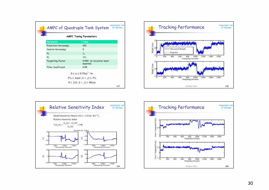
Automation LabIIT BombayAMPC of Quadruple Tank System
Parameter Value
Prediction Horizon(p) 100
Control Horizon(q) 5
�� ��
�� 10��
Forgetting Factor 0.999 (in recursive least squares)
Filter Coefficient 0.95
117
40cm)|(ˆ0
3%)|u(3%
/0.95mu0 3
jkky
jkk
hr
AMPC Tuning Parameters
Automation LabIIT BombayTracking Performance
ACODS 2016 118
Automation LabIIT BombayRelative Sensitivity Index
119
100)0(
)0()()(%
Index Sensitvity Relative
]-I)[()(y Matrix Sensitivit Model u1
ij
ijijij
G
GkGkS
kCkG
Automation LabIIT BombayTracking Performance
120ACODS 2016
31
Automation LabIIT Bombay
1219/18/2016 State Feedback Control 121
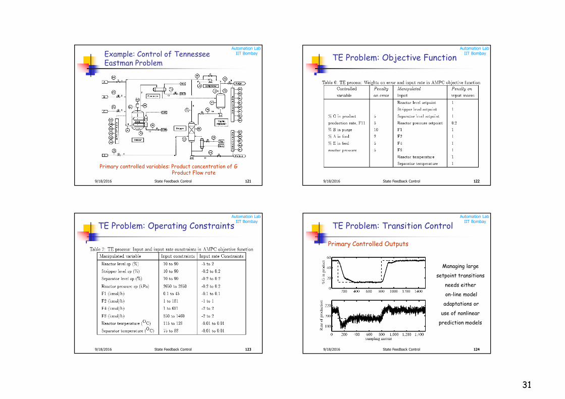
Example: Control of Tennessee Eastman Problem
Primary controlled variables: Product concentration of GProduct Flow rate
Automation LabIIT Bombay
1229/18/2016 State Feedback Control 122
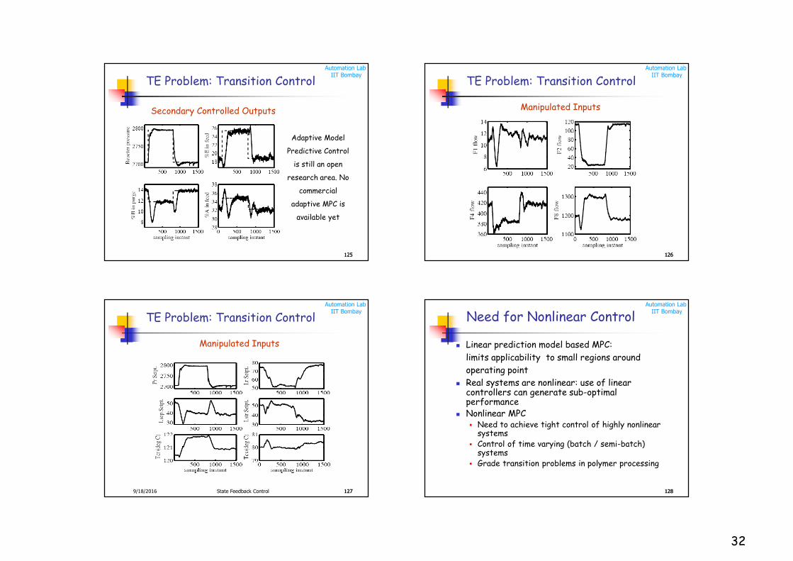
TE Problem: Objective Function
Automation LabIIT Bombay
1239/18/2016 State Feedback Control 123
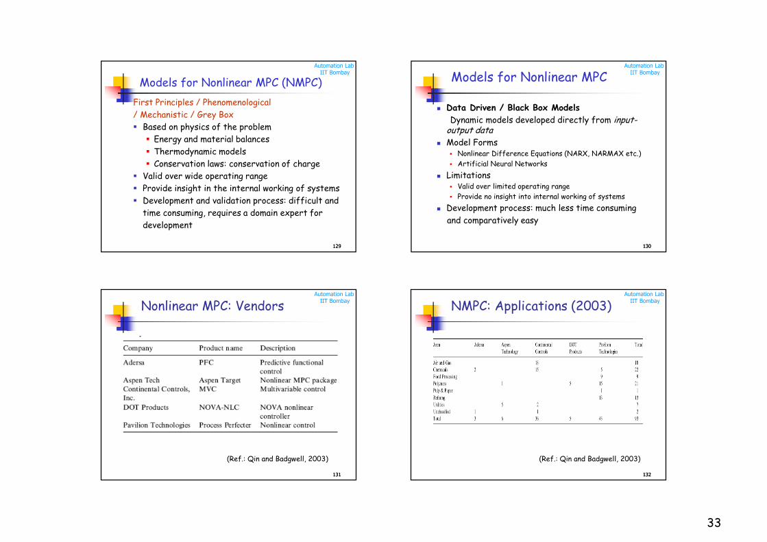
TE Problem: Operating Constraints
Automation LabIIT Bombay
1249/18/2016 State Feedback Control 124
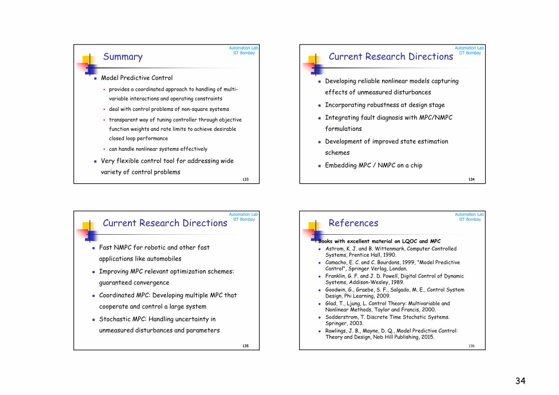
TE Problem: Transition Control
Primary Controlled Outputs
Managing large
setpoint transitions
needs either
on-line model
adaptations or
use of nonlinear
prediction models
32
Automation LabIIT Bombay
125125
TE Problem: Transition Control
Secondary Controlled Outputs
Adaptive Model
Predictive Control
is still an open
research area. No
commercial
adaptive MPC is
available yet
Automation LabIIT Bombay
126126
TE Problem: Transition Control
Manipulated Inputs
Automation LabIIT Bombay
1279/18/2016 State Feedback Control 127
TE Problem: Transition Control
Manipulated Inputs
Automation LabIIT Bombay
128128
Need for Nonlinear Control
Linear prediction model based MPC:
limits applicability to small regions around
operating point
Real systems are nonlinear: use of linear controllers can generate sub-optimal performance
Nonlinear MPC Need to achieve tight control of highly nonlinear
systems
Control of time varying (batch / semi-batch) systems
Grade transition problems in polymer processing
33
Automation LabIIT Bombay
129129
Models for Nonlinear MPC (NMPC)
First Principles / Phenomenological
/ Mechanistic / Grey Box
Based on physics of the problem
Energy and material balances
Thermodynamic models
Conservation laws: conservation of charge
Valid over wide operating range
Provide insight in the internal working of systems
Development and validation process: difficult and
time consuming, requires a domain expert for
development
Automation LabIIT Bombay
130130
Models for Nonlinear MPC
Data Driven / Black Box Models
Dynamic models developed directly from input-output data
Model Forms Nonlinear Difference Equations (NARX, NARMAX etc.)
Artificial Neural Networks
Limitations Valid over limited operating range
Provide no insight into internal working of systems
Development process: much less time consuming
and comparatively easy
Automation LabIIT Bombay
131131
Nonlinear MPC: Vendors
(Ref.: Qin and Badgwell, 2003)
Automation LabIIT Bombay
132132
NMPC: Applications (2003)
(Ref.: Qin and Badgwell, 2003)
34
Automation LabIIT Bombay
133133
Summary
Model Predictive Control
provides a coordinated approach to handling of multi-
variable interactions and operating constraints
deal with control problems of non-square systems
transparent way of tuning controller through objective
function weights and rate limits to achieve desirable
closed loop performance
can handle nonlinear systems effectively
Very flexible control tool for addressing wide
variety of control problems
Automation LabIIT Bombay
134134
Current Research Directions
Developing reliable nonlinear models capturing
effects of unmeasured disturbances
Incorporating robustness at design stage
Integrating fault diagnosis with MPC/NMPC
formulations
Development of improved state estimation
schemes
Embedding MPC / NMPC on a chip
Automation LabIIT Bombay
135135
Current Research Directions
Fast NMPC for robotic and other fast
applications like automobiles
Improving MPC relevant optimization schemes:
guaranteed convergence
Coordinated MPC: Developing multiple MPC that
cooperate and control a large system
Stochastic MPC: Handling uncertainty in
unmeasured disturbances and parameters
Automation LabIIT Bombay
136
References
Books with excellent material on LQOC and MPC
Astrom, K. J. and B. Wittenmark, Computer Controlled Systems, Prentice Hall, 1990.
Camacho, E. C. and C. Bourdons, 1999, "Model Predictive Control", Springer Verlag, London.
Franklin, G. F. and J. D. Powell, Digital Control of Dynamic Systems, Addison-Wesley, 1989.
Goodwin, G., Graebe, S. F., Salgado, M. E., Control System Design, Phi Learning, 2009.
Glad, T., Ljung, L. Control Theory: Multivariable and Nonlinear Methods, Taylor and Francis, 2000.
Sodderstrom, T. Discrete Time Stochstic Systems. Springer, 2003.
Rawlings, J. B., Mayne, D. Q., Model Predictive Control: Theory and Design, Nob Hill Publishing, 2015.
35
Automation LabIIT Bombay
137
References
MPC and Related Important Review Articles
Garcia, C. E., Prett, D. M. , Morari, M. Model predictive control: Theory and practice - A survey. Automatica, 25 (1989), 335-348.
Morari, M. , Lee, J.H., Model Predictive Control: Past, Present and Future, Comp. Chem. Engg., 23 (1999), 667-682.
Henson, M.A. (1998). Nonlinear Model Predictive Control : Current status and future directions. Computers and Chemical Engg,23 , 187- 202.
Lee, J.H. (1998). Modeling and Identification for Nonlinear Model Predictive control:Requirements present status and future needs. International Symposium on Nonlinear Model Predictive control,Ascona, Switzerland.
Meadows, E.S. , Rawlings, J. B. Nonlinear Process Control, ( M.A. Henson and D.E. Seborg (eds.), New Jersey: Prentice Hall, Chapter 5.(1997).
Qin, S.J., Badgwell, T.A. A servey of industrial model predictive control technology, Control Engineering Practice 11 (2003) 733-764.
Automation LabIIT Bombay
138
References
Useful / Important Papers
Muske, K. R. , Rawlings, J. B. ; Model Predictive control with linear models, AIChE J., 39 (1993), 262-287.
Muske, K. R. ;Badgwell, T. A. Disturbance modeling for offset-free linear model predictive control. Journal of Process Control, 12 (2002), 617-632.
Ricker, N. L., Model Predictive Control with State Estimation, Ind. Eng. Chem. Res., 29 (1990), 374-382.
Yu, Z. H. , Li , W., Lee, J.H. , Morari, M. State Estimation Based Model Predictive Control applied to Shell Control Problem: A Case Study, Chem. Eng. Sci., (1994), 14-22.
Patwardhan S.C. and S.L. Shah (2005) From data to diagnosis and control using generalized orthonormal basis filters. Part I: Development of state observers, Journal of Process Control,15,7, 819-835.
Automation LabIIT Bombay
References
Srinivas, K., Shaw, R., Patwardhan, S. C., Noronha, S. Adaptive model predictive control of multivariable time-varying systems. Ind. Eng. Chem. Res., 2008, 47, 2708-2720.
Badwe, A., Singh, A., Patwardhan, S. C., Gudi. R. D., A Constrained Recursive Pseudo-linear Regression Scheme for On-line Parameter Estimation in Adaptive Control. Journal of Process Control, 20, 559–572, 2010.
Srinivasarao,M.; Patwardhan,S. C.; Gudi, R. D. Nonlinear predictive control of irregularly sampled multi-rate systems using nonlinear black box observers. Journal of Process Control, 2007, 17, 17–35.
Srinivasrao, M.; Patwardhan, S.C. ; Gudi, R. D. From data to nonlinear predictive control. 2.. Improving regulatory performance using identified observers. Ind. Eng. Chem. Res., 2006, 45, 3593-3603.
139
Automation LabIIT Bombay
References
Prakash, J.; Patwardhan, S. C.;Narasimhan, S. Integrating model based fault diagnosis with model predictive control. Ind. Eng. Chem. Res., 2005, 44, 4344-4360.
Patwardhan, S.C. ; Manuja, S.; Narasimhan, S.; Shah, S. L From data to diagnosis and control using generalized orthonormal basis filters. Part II: Model predictive and fault tolerant control. Journal of Process Control, 2006, 16, 157–175.
Deshpande, A., Patwardhan, S. C., Narasimhan, S. Intelligent State Estimation for Fault Tolerant Nonlinear Model Predictive Control, Journal of Process Control, 19, 187–204, 2009.
140