54

Bearing-capacity prediction of spatially randomc − φ soils

Gordon A. Fenton and D.V. Griffiths

Abstract: Soils with spatially varying shear strengths are modeled using random field theory and elasto-plastic finiteelement analysis to evaluate the extent to which spatial variability and cross-correlation in soil properties (c and φ) affectbearing capacity. The analysis is two dimensional, corresponding to a strip footing with infinite correlation length inthe out-of-plane direction, and the soil is assumed to be weightless with footing placed on the soil surface. Theoreticalpredictions of the mean and standard deviation of bearing capacity, for the case where c and φ are independent, arederived using a geometric averaging model and then verified via Monte Carlo simulation. The standard deviationprediction is found to be quite accurate, while the mean prediction is found to require some additional semi-empiricaladjustment to give accurate results for “worst case” correlation lengths. Combined, the theory can be used to estimate theprobability of bearing-capacity failure, but also sheds light on the stochastic behaviour of foundation bearing failure.

Key words: bearing capacity, probability, random fields, geometric averaging, c–φ soil, Monte Carlo simulation.

Résumé : Les sols ayant des résistances au cisaillement variables dans l’espace sont modélisés au moyen de la théorie dechamp aléatoire et d’une analyse élasto-plastique en éléments finis pour évaluer jusqu’à quel point la variabilité spatiale etla corrélation en travers dans les propriétés des sols (c et φ) influence la capacité portante. L’analyse est bidimensionnelle,correspondant à une semelle filante avec une longueur infinie de corrélation dans la direction sortant du plan, et le sol estsupposé être sans poids avec la semelle placée sur la surface du sol. On dérive les prédictions théoriques des déviationsmoyenne et standard de la capacité portante, pour le cas où c et sont indépendants, en utilisant un modèle de moyennegéométrique, et elles sont ensuite vérifiées par la simulation de Monte Carlo. On trouve que la prédiction de la déviationstandard est très précise, alors que la prédiction de la moyenne requiert des ajustements semi-empiriques additionnels pourdonner des résultats précis pour le « pire cas » de longueurs corrélées. En combinaison, la théorie peut être utilisée pourestimer la probabilité de rupture en capacité portante, mais elle éclaircit aussi le comportement stochastique de la ruptureen portance des fondations.

Mots clés : capacité portante, probabilité, champs aléatoires, moyenne géométrique de c–φ du sol, simulation de MonteCarlo.

[Traduit par la Rédaction]

Introduction

The design of a footing involves two limit states: a service-ability limit state, which generally translates into a maximumsettlement or differential settlement, and an ultimate limit state.The latter is concerned with the maximum load that can beplaced on the footing just prior to a bearing-capacity failure.This paper looks at the ultimate bearing capacity of a smoothstrip footing founded on a soil having spatially random proper-ties.

Most modern bearing-capacity predictions involve a relation-ship of the form (Terzaghi 1943)

[1] qf = cNc + qNq + 12γBNγ

where qf is the ultimate bearing stress, c is the cohesion, q is

Received 6 February 2002. Accepted 11 July 2002. Published onthe NRC Research Press Web site at http://cgj.nrc.ca/ on 16 January2003.

G.A. Fenton.1 Dalhousie University, Halifax, NS B3J 2X4, Canada.D.V. Griffiths. Colorado School of Mines, Golden, CO 80401,U.S.A.

1 Corresponding author (e-mail: Gordon.Fenton@dal.ca).

the overburden stress, γ is the unit soil weight, B is the footingwidth, and Nc, Nq , and Nγ are the bearing-capacity factors.To simplify the analysis in this paper, and to concentrate onthe stochastic behaviour of the most important term (at leastas far as spatial variation is concerned), the soil is assumedto be weightless. Under this assumption, the bearing-capacityequation simplifies to

[2] qf = cNc

Bearing-capacity predictions, involving specification of theN factors, are often based on plasticity theory (see, e.g., Prandtl1921; Terzaghi 1943; Sokolovski 1965) of a rigid base punchinginto a softer material. These theories assume a homogeneoussoil underlying the footing, that is, the soil is assumed to haveproperties that are spatially constant. Under this assumption,most bearing-capacity theories (e.g., Prandtl 1921; Meyerhof1951, 1963) assume that the failure slip surface takes on a log-arithmic spiral shape to give

[3] Nc =eπ tan φ tan2

(π4 + φ

2

)− 1

tan φ

This relationship has been found to give reasonable agree-ment with test results (Bowles 1996) under ideal conditions.

Can. Geotech. J. 40: 54–65 (2003) doi: 10.1139/T02-086 © 2003 NRC Canada

Fenton and Griffiths 55

In practice, however, it is well known that the actual failureconditions will be somewhat more complicated than a simplelogarithmic spiral. Because of spatial variation in soil propertiesthe failure surface under the footing will follow the weakest paththrough the soil, constrained by the stress field. For example,Fig. 1 illustrates the bearing failure of a realistic soil with spa-tially varying properties. It can be seen that the failure surfaceonly approximately follows a log spiral on the right side and iscertainly not symmetric. In this plot lighter regions representstronger soil and darker regions indicate weaker soil. The weak(dark) region near the ground surface to the right of the footinghas triggered a nonsymmetric failure mechanism that is typi-cally at a lower bearing load than that predicted by traditionalhomogeneous and symmetric failure analysis.

The problem of finding the minimum strength failure slipsurface through a soil mass is very similar in nature to the slopestability problem, and one that currently lacks a closed formstochastic solution, so far as the authors are aware. In this pa-per the traditional relationships shown above will be used as astarting point to this problem.

For a realistic soil, both c and φ are random, so that bothquantities in the right hand side of eq. [2] are random. Thisequation can be nondimensionalized by dividing through bythe cohesion mean,

[4] Mc = qf

µc

= c

µc

Nc

where µc is the mean cohesion and Mc is the stochastic equiv-alent of Nc, i.e., qf = µcMc. The stochastic problem is nowboiled down to finding the distribution of Mc. A theoreticalmodel for the first two moments (mean and variance) of Mc,based on geometric averaging, are given in the next section.Monte Carlo simulations are then performed to assess the qual-ity of the predictions and determine the approximate form ofthe distribution of Mc. This is followed by an example illustrat-ing how the results can be used to compute the probability ofa bearing-capacity failure. Finally, an overview of the results isgiven, including their limitations.

The random soil model

In this study, the soil cohesion, c, is assumed to be lognor-mally distributed with mean µc, standard deviation σc, andspatial correlation length θln c. The lognormal distribution isselected because it is commonly used to represent non-negativesoil properties and has a simple relationship with the normal.A lognormally distributed random field is obtained from a nor-mally distributed random field,Gln c(x∼), having zero mean, unit

variance, and spatial correlation length θln c through the trans-formation

[5] c(x∼) = exp[µln c + σln cGln c(x∼)]

where x∼ is the spatial position at which c is desired. The pa-

rametersµln c and σln c are obtained from the specified cohesion

mean and variance using the lognormal distribution transforma-tions,

σ 2ln c = ln

(1 + σ 2

c

µ2c

)[6a]

µln c = lnµc − 12σ

2ln c[6b]

The correlation coefficient between the log cohesion at apoint x∼1 and a second point x∼2 is specified by a correlation

function, ρln c(τ ), where τ = |x∼1 − x∼2| is the absolute distance

between the two points. In this paper, a simple exponentiallydecaying (Markovian) correlation function will be assumed,having the form

[7] ρln c(τ ) = exp

(−2|τ |θln c

)

The spatial correlation length, θln c, is loosely defined as theseparation distance within which two values of ln c are signifi-cantly correlated. Mathematically, θln c is defined as the area un-der the correlation function, ρln c(τ ) (Vanmarcke 1984). (Notethat geostatisticians often define the correlation length as thearea under the non-negative half of the correlation function sothat there is a factor of two difference between the two lengths;under their definition, the factor of 2 appearing in eq. [7] is ab-sent. The more general definition is retained here since it can beused also in higher dimensions where the correlation functionis not necessarily symmetric in all directions about the origin.)

It should also be noted that the correlation function selectedabove acts between values of ln c. This is because ln c is nor-mally distributed, and a normally distributed random field issimply defined by its mean and covariance structure. In prac-tice, the correlation length θln c can be estimated by evaluatingspatial statistics of the log-cohesion data directly (see, e.g., Fen-ton 1999). Unfortunately, such studies are scarce, so that littleis currently known about the spatial correlation structure of nat-ural soils. For the problem considered here, it turns out that aworst case correlation length exists that should be assumed inthe absence of improved information.

The random field is also assumed here to be statisticallyisotropic (the same correlation length in any direction throughthe soil). Although the horizontal correlation length is oftengreater than the vertical, because of soil layering, taking thisinto account was deemed to be a refinement beyond the scopeof this study. The main aspects of the stochastic behaviour ofbearing capacity needs to be understood for the simplest casefirst, and more complex variations on the theme, such as sitespecific anisotropy, left for later work.

The friction angle, φ, is assumed to be bounded both aboveand below, so that neither normal nor lognormal distributionsare appropriate. A beta distribution is often used for boundedrandom variables. Unfortunately, a beta-distributed random fieldhas a very complex joint distribution, and simulation is cum-bersome and numerically difficult. To keep things simple, abounded distribution is selected that resembles a beta distri-bution but that arises as a simple transformation of a standardnormal random field, Gφ(x∼), according to

©2003 NRC Canada

56 Can. Geotech. J. Vol. 40, 2003

Fig. 1. Typical deformed mesh at failure, where the darker regions indicate weaker soil.

[8] φ(x∼) = φmin + 12 (φmax −φmin)

[1 + tanh

(sGφ(x∼)

2π

)]

where φmin and φmax are the minimum and maximum frictionangles, respectively, and s is a scale factor that governs the fric-tion angle variability between its two bounds. Figure 2 showshow the distribution of φ (normalized to the interval [0, 1])changes as s changes, going from an almost uniform distribu-tion at s = 5 to a very normal looking distribution for smallervalues of s. In all cases, the distribution is symmetric, so thatthe midpoint between φmin and φmax is the mean. Values of sgreater than about 5 lead to a U-shaped distribution (higher atthe boundaries), which is not deemed realistic. Thus, varying sbetween about 0.1 and 5.0 leads to a wide range in the stochasticbehaviour of φ.

The random field,Gφ(x∼), has zero mean and unit variance, as

doesGln c(x∼). Conceivably,Gφ(x∼) could also have its own cor-

relation length θφ distinct from θln c. However, it seems reason-able to assume that if the spatial correlation structure is causedby changes in the constitutive nature of the soil over space, thenboth cohesion and friction angle would have similar correlationlengths. Thus, θφ is taken to be equal to θln c in this study. Bothlengths will be referred to generically from now on simply as θ ,remembering that this length reflects correlation between pointsin the underlying normally distributed random fields, Gln c(x∼)and Gφ(x∼), and not directly between points in the cohesion

and friction fields. As mentioned above, both lengths can beestimated from data sets obtained over some spatial domain bystatistically analyzing the suitably transformed data (inversesof eqs. [5] and [8]). After transforming to the c and φ fields, thetransformed correlation lengths will no longer be the same, butsince both transformations are monotonic (i.e., larger values ofGln c give larger values of c, etc.), the correlation lengths willbe similar (for s = 1.0, the difference is less than 15% fromeach other and from the original correlation length). In that allengineering soil properties are derived through various transfor-mations of the physical soil behaviour (e.g., cohesion is a com-plex function of electrostatic forces between soil particles), thefinal correlation lengths between engineering properties can-

not be expected to be identical, only similar. For the purposesof a generic non-site specific study, the above assumptions arebelieved reasonable.

The question as to whether the two parameters c and φ arecorrelated is still not clearly decided in the literature, and nodoubt depends very much on the soil being studied. Cherubini(2000) quotes values of ρ ranging from −0.24 to −0.70, asdoes Wolff (1985) (see also Yuceman et al. 1973; Lumb 1970;Cherubini 2000). As stated by Wolff (T.H. Wolff, private cor-respondence, 2000): “The practical meaning of this [negativecorrelation] is that we are more certain of the undrained strengthat a certain confining pressure than the values of the two pa-rameters we use to define it.” This observation arises from thefact that the variance of the shear strength is reduced if there isa negative correlation between c and φ.

In that the correlation between c and φ is not certain, this pa-per investigates the correlation extremes to determine if cross-correlation makes a significant difference.As will be seen, underthe given assumptions regarding the distributions of c (lognor-mal) and φ (bounded), varying the cross-correlation ρ from −1to 1 was found to have only a minor influence on the stochasticbehaviour of the bearing capacity.

Bearing-capacity mean and variance

The determination of the first two moments of the bearingcapacity (mean and variance) requires first a failure model.Equations [2] and [3] assume that the soil properties are spa-tially uniform. When the soil properties are spatially varying,the slip surface no longer follows a smooth log spiral, and thefailure becomes unsymmetric. The problem of finding the con-strained path having the lowest total shear strength through thesoil is mathematically difficult, especially since the constraintsare supplied by the stress field. A simpler approximate modelwill be considered here wherein geometric averages of c andφ, over some region under the footing, are used in eqs. [2] and[3]. The geometric average is proposed because it is dominatedmore by low strengths than is the arithmetic average. This isdeemed reasonable since the failure slip surface preferentiallytravels through lower strength areas.

Consider a soil region of some size D discretized into a se-quence of non-overlapping rectangles, each centered on x∼i , i =

©2003 NRC Canada

Fenton and Griffiths 57

Fig. 2. Bounded distribution of friction angle normalized to the interval [0, 1].

1, 2, . . . , n. The geometric average of the cohesion, c, over thedomain D may then be defined as

[9] c =[

n∏i=1

c(x∼ i )

]1/n

= exp

[1

n

n∑i=1

ln c(x∼ i )

]

= exp(µln c + σln cGln c

)where Gln c is the arithmetic average of Gln c over the domainD. Note that an assumption is made in the above concerningc(x∼i ) being constant over each rectangle. In that cohesion is

generally measured using some representative volume (e.g., alaboratory sample), the values of c(x∼i ) used above are deemed

to be such measures.In a similar way, the exact expression for the geometric av-

erage of φ over the domain D is

[10] φ = exp

[1

n

n∑i=1

ln φ(x∼ i )

]

where φ(x∼i ) is evaluated using eq. [8]. A close approximation

to the above geometric average, accurate for s ≤ 2.0, is

[11] φ φmin + 12 (φmax − φmin)

[1 + tanh

(sGφ

2π

)]

where Gφ is the arithmetic average of Gφ over the domain D.For φmin = 5◦ and φmax = 45◦, this expression has relativeerror of less than 5% for n = 20 independent samples. Whilethe relative error rises to about 12%, on average, for s = 5.0,this is an extreme case, corresponding to a uniformly distributedφ between the minimum and maximum values, which is felt tobe unlikely to occur very often in practice. Thus, the aboveapproximation is believed reasonable in most cases.

Using the latter result in eq. [3] gives the “effective” value ofNc, Nc, where the log-spiral model is assumed to be valid usinga geometric average of soil properties within the failed region,

[12] Nc =eπ tan φ tan2

(π4 + φ

2

)− 1

tan φ

so that, now

[13] Mc = c

µc

Nc

If c is lognormally distributed, an inspection of eq. [9] indi-cates that c is also lognormally distributed. If we can assumethat Nc is at least approximately lognormally distributed, thenMc will also be at least approximately lognormally distributed(the central limit theorem helps out somewhat here). In thiscase, taking logarithms of eq. [13] gives

[14] lnMc = ln c + ln Nc − lnµc

so that, under the given assumptions, lnMc is at least approxi-mately normally distributed.

The task now is to find the mean and variance of lnMc. Themean is obtained by taking expectations of eq. [14],

[15] µlnMc = µln c + µln Nc− lnµc

where

[16] µln c = E[µln c + σln cGln c

]= µln c + σln cE

[Gln c

]= µln c

= lnµc − 12 ln

(1 + σ 2

c

µ2c

)

which used the fact that since Gln c is normally distributed, itsarithmetic average has the same mean asGln c, that is E

[Gln c

] =

©2003 NRC Canada

58 Can. Geotech. J. Vol. 40, 2003

E [Gln c] = 0. The above result is as expected since the geo-metric average of a lognormally distributed random variablepreserves the mean of the logarithm of the variable. Also eq.[6b] was used to express the mean in terms of the prescribedstatistics of c.

A second-order approximation to the mean of the logarithmof eq. [12], µln Nc

, is

[17] µln Nc ln Nc(µφ) + σ 2

φ

(d2 ln Nc

dφ2

∣∣∣µφ

)

where µφ is the mean of the geometric average of φ. Since

Gφ is an arithmetic average, its mean is equal to the mean ofGφ , which is zero. Thus, since the assumed distribution of φis symmetric about its mean, µφ = µφ so that ln Nc(µφ) =lnNc(µφ).

A first-order approximation to σ 2φ

is

[18] σ 2φ

=[ s

4π(φmax − φmin)σGφ

]2

where, from local averaging theory (Vanmarcke 1984), the vari-ance of a local average over the domainD is given by (recallingthat Gφ is normally distributed with zero mean and unit vari-ance),

[19] σ 2Gφ

= σ 2Gφ

γ (D) = γ (D)

where γ (D) is the “variance function” that reflects the amountby which the variance is reduced as a result of local arithmeticaveraging. It can be obtained directly from the correlation func-tion (see Appendix A).

The derivative in eq. [17] is most easily obtained numericallyusing any reasonably accurate (Nc is quite smooth) approxima-tion to the second derivative (see, e.g., Press et al. 1997). Ifµφ = µφ = 25◦ = 0.436 rad (note that in all mathematicalexpressions, φ is assumed to be in radians), then

[20]d2 ln Nc

dφ2

∣∣∣µφ

= 5.2984 rad−2

Using these results with φmax = 45◦ and φmin = 5◦, so thatµφ = 25◦ gives

[21] µln Nc= ln(20.72) + 0.0164s2γ (D)

Some comments need to be made about this result: first ofall it increases with increasing variability in φ (increasing s). Itseems doubtful that this increase would occur since increasingvariability in φ would likely lead to more lower strength pathsthrough the soil mass for moderate θ . Aside from ignoring theweakest path issue, some other sources of error in the aboveanalysis are

(1) The geometric average of φ given by eq. [10] actuallyshows a slight decrease with s (about 12% less, relatively,when s = 5). Although the decrease is only slight, it atleast is in the direction expected.

(2) An error analysis of the second-order approximation ineq. [17] and the first-order approximation in eq. [18] hasnot been carried out. Given the rather arbitrary natureof the assumed distribution on φ, and the fact that thispaper is primarily aimed at establishing the approximatestochastic behaviour, such refinements have been left forlater work.

In light of these observations, a first-order approximation toµln Nc

may actually be more accurate. Namely

[22] µln Nc ln Nc(µφ) lnNc(µφ)

Finally, combining eqs. [16] and [22] into eq. [15] gives

[23] µlnMc lnNc(µφ) − 12 ln

(1 + σ 2

c

µ2c

)

For independent c and φ, the variance of lnMc is

[24] σ 2lnMc

= σ 2ln c + σ 2

ln Nc

where

[25] σ 2ln c = γ (D)σ 2

ln c = γ (D) ln

(1 + σ 2

c

µ2c

)

and, to first order,

[26] σ 2ln Nc

σ 2φ

(d ln Nc

dφ

∣∣∣µφ

)2

The derivative appearing in eq. [26], which will be denotedas β(φ), is

[27] β(φ) = d ln Nc

dφ= d lnNc

dφ

= bd

bd2 − 1

[π(1 + a2)d + 1 + d2

]− 1 + a2

a

where a = tan(φ), b = eπa , and d = tan(π4 + φ

2

).

The variance of lnMc is thus

[28] σ 2lnMc

γ (D)

×{

ln

(1 + σ 2

c

µ2c

)+[( s

4π

)(φmax − φmin)β(µφ)

]2}

where φ is measured in radians.

Monte Carlo simulation

A finite-element computer program was written to computethe bearing capacity of a smooth rigid strip footing (plane strain)founded on a weightless soil with shear strength parametersc and φ represented by spatially varying and cross-correlated(point-wise) random fields, as discussed above. The bearing-capacity analysis uses an elastic-perfectly plastic stress–strainlaw with a classical Mohr–Coulomb failure criterion. Plastic

©2003 NRC Canada

Fenton and Griffiths 59

Table 1. Random field parametersused in the study.

Parameter Valueθ 0.5, 1.0, 2.0, 4.0, 8.0, 50COV 0.1, 0.2, 0.5, 1.0, 2.0, 5.0ρ –1.0, 0.0, 1.0

stress redistribution is accomplished using a viscoplastic algo-rithm. The program uses eight-node quadrilateral elements andreduced integration in both the stiffness and stress redistributionparts of the algorithm. The theoretical basis of the method is de-scribed more fully in Chap. 6 of the text by Smith and Griffiths(1998). The finite-element model incorporates five parameters:Young’s modulus (E), Poisson’s ratio (ν), dilation angle (ψ),shear strength (c), and friction angle (φ). The program allowsfor random distributions of all five parameters; however, in thepresent study,E, ν, andψ are held constant (at 100 000 kN/m2,0.3, and 0, respectively) while c and φ are randomized. TheYoung’s modulus governs the initial elastic response of the soil,but does not affect bearing capacity. Setting the dilation angleto zero means that there is no plastic dilation during yield ofthe soil. The finite element mesh consists of 1000 elements, 50elements wide by 20 elements deep. Each element is a 0.1 ×0.1 m square, and the strip footing occupies 10 elements, givingit a width of B = 1 m.

The random fields used in this study are generated using thelocal average subdivision method (Fenton 1994; Fenton andVanmarcke 1990). Cross-correlation between the two soil prop-erty fields (c and φ) is implemented via covariance matrix de-composition (Fenton 1994). The algorithm is given inAppendixB.

In the parametric studies that follow, the mean cohesion(µc) and mean friction angle (µφ) have been held constant at100 kN/m2 and 25◦ (with φmin = 5◦ and φmax = 45◦), respec-tively, while the COV (= σc/µc), spatial correlation length (θ ),and correlation coefficient, ρ, between Gln c and Gφ are variedsystematically according to Table 1.

It will be noticed that COVs up to 5.0 are considered in thisstudy, which is an order of magnitude higher than generallyreported in the literature (see, e.g., Phoon and Kulhawy 1999).There are two considerations that complicate the problem ofdefining typical COVs for soils that have not yet been clearlyconsidered in the literature (although Fenton (1999) does intro-duce these issues). The first has to do with the level of informa-tion known about a site. Prior to any site investigation, there willbe plenty of uncertainty about soil properties, and an appropri-ate COV comes by using a COV obtained from regional dataover a much larger scale. Such a COV will typically be muchgreater than that found when soil properties are estimated overa much smaller scale, such as a specific site. As investigationproceeds at the site of interest, the COV drops. For example, asingle sample at the site will reduce the COV slightly, but as theinvestigation intensifies, the COV drops towards zero, reachingzero when the entire site has been sampled (which, of course, isclearly impractical). The second consideration, which is actu-ally closely tied to the first, has to do with scale. If one were totake soil samples every 10 km over 5000 km (macroscale), onewill find that the COV of those samples will be very large. ACOV of 5.0 would not be unreasonable. Alternatively, suppose

one were to concentrate one’s attention on a single cubic metreof soil. If several 50 mm2 samples were taken and sent to thelaboratory, one would expect a fairly small COV. On the otherhand, if samples of size 0.1 µm3 were taken and tested (assum-ing this was possible), the resulting COV could be very large,since some samples might consist of very hard rock particles,others of water, and others just of air (i.e., the sample locationfalls in a void). In such a situation, a COV of 5.0 could easilybe on the low side. While the last scenario is only conceptual, itdoes serve to illustrate that COV is highly dependent on the ratiobetween sample volume and sampling domain volume. This de-pendence is certainly pertinent to the study of bearing capacity,since it is currently not known at what scale bearing-capacityfailure operates. Is the weakest path through a soil dependenton property variations at the microscale (having a large COV)or does the weakest path “smear” the small-scale variations anddepend primarily on local average properties over, say, labora-tory scales (small COV)? Since laboratory scales are merelyconvenient for us, it is unlikely that nature has selected thatparticular scale to accommodate us. From the point of view ofreliability estimates, where the failure mechanism might de-pend on microscale variations for failure initiation, the smallCOVs reported in the literature might very well be dangerouslyunconservative. Much work is still required to establish the re-lationship between COV, site investigation intensity, and scale.In the meantime, this paper considers COVs over a fairly widerange, since it is entirely possible that the higher values moretruly reflect failure variability.

In addition, it is assumed that when the variability in thecohesion is large, the variability in the friction angle will alsobe large. Under this reasoning, the scale factor, s, used in eq.[8] is set to s = σc/µc = COV. This choice is arbitrary, butresults in the friction angle varying from quite narrowly (whenCOV = 0.1 and s = 0.1) to very widely (when COV = 5.0and s = 5) between its lower and upper bounds, 5◦ and 45◦, asillustrated in Fig. 2.

For each set of assumed statistical properties given by Ta-ble 1, Monte Carlo simulations have been performed. Theseinvolve 1000 realizations of the soil property random fields andthe subsequent finite-element analysis of bearing capacity. Eachrealization, therefore, has a different value of the bearing capac-ity and, after normalization by the mean cohesion, a differentvalue of the bearing-capacity factor,

[29] Mci = qfi

µc

, i = 1, 2, . . . , 1000

=⇒ µlnMc = 1

1000

1000∑i=1

lnMci

where µlnMc is the sample mean of lnMc estimated over theensemble of realizations. Because of the non-linear nature of theanalysis, the computations are quite intensive. One run of 1000realizations typically takes about 2 days on a dedicated 800-MHz Pentium� III computer (which, by the time of printing,is likely obsolete). For the 108 cases considered in Table 1,the total single CPU time required is about 220 days (run timevaries with the number of iterations required to analyze variousrealizations).

©2003 NRC Canada

60 Can. Geotech. J. Vol. 40, 2003

Fig. 3. (a) Sample mean of log bearing-capacity factor, lnMc, and (b) its sample standard deviation.

Simulation resultsFigure 3a shows how the sample mean log bearing-capacity

factor, taken as the average over the 1000 realizations of lnMciand referred to as µlnMc in Fig. 3, varies with correlation length,soil variability, and cross-correlation between c andφ. For smallsoil variability, µlnMc tends towards the deterministic valueof ln(20.72) = 3.03, which is found when the soil takes onits mean properties everywhere. For increasing soil variability,the mean bearing-capacity factor becomes quite significantlyreduced from the traditional case. What this implies from adesign standpoint is that the bearing capacity of a spatiallyvariable soil will, on average, be less than the Prandtl solu-tion based on the mean values alone. The greatest reductionfrom the Prandtl solution is observed for perfectly correlatedc and φ (ρ = 1), the least reduction when c and φ are nega-tively correlated (ρ = −1), and the independent case (ρ = 0)lies between these two extremes. However, the effect of cross-correlation is seen to be not particularly large. If the negativecross-correlation indicated by both Cherubini (2000) and Wolff(1985) is correct, then the independent, ρ = 0, case is conser-vative, having mean bearing capacities consistently somewhatless than the ρ = −1 case.

The cross-correlation between c and φ is seen to have min-imal effect on the sample standard deviation, σlnMc , as shownin Fig. 3b. The sample standard deviation is most strongly af-fected by the correlation length and somewhat less so by the soilproperty variability. A decreasing correlation length results in adecreasing σlnMc . As suggested by eq. [28], the function γ (D)decays approximately with θ/D and so decreases with decreas-ing θ . This means that σlnMc should decrease as the correlationlength decreases, which is as seen in Fig. 3b.

Figure 3a also seems to show that the correlation length,θ , does not have a significant influence in that the θ = 0.1and θ = 8 curves for ρ = 0 are virtually identical. However,the θ = 0.1 and θ = 8 curves are significantly lower thanthat predicted by eq. [23] implying that the plot is somewhatmisleading with respect to the dependence on θ . For example,

when the correlation length goes to infinity, the soil proper-ties become spatially constant, albeit still random from real-ization to realization. In this case, because the soil propertiesare spatially constant, the weakest path returns to the log spi-ral and µlnMc will rise towards that given by eq. [23], namelyµlnMc = ln(20.72)− 1

2 ln(1+σ 2c /µ

2c), which is also shown on

the plot. This limiting value holds because µlnNc lnNc(µφ),as discussed for eq. [22], where for spatially constant propertiesφ = φ.

Similarly, when θ → 0, the soil property field becomes in-finitely “rough”, in that all points in the field become indepen-dent. Any point at which the soil is weak will be surroundedby points where the soil is strong. A path through the weak-est points in the soil might have very low average strength, butat the same time will become infinitely tortuous and thus in-finitely long. This, combined with shear interlocking dictatedby the stress field, implies that the weakest path should returnto the traditional log spiral with average shear strength alongthe spiral given byµc andµφ . Again, in this case,µlnMc shouldrise to that given by eq. [23].

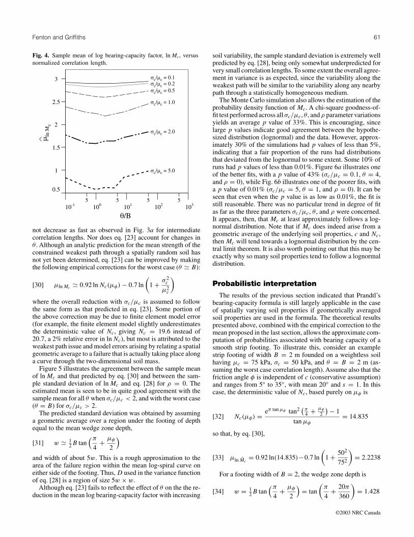
The variation of µlnMc with respect to θ is more clearly seenin Fig. 4. Over a range of values of σc/µc, the value of µlnMc

rises towards that predicted by eq. [23] at both high and low cor-relation lengths. At intermediate correlation lengths, the weak-est path issue is seen to result in µlnMc being less than thatpredicted by eq. [23] (see Fig. 3a), the greatest reduction inµlnMc occurring when θ is of the same order as the footingwidth, B. It is hypothesized that θ B leads to the greatestreduction in µlnMc because it allows enough spatial variabilityfor a failure surface that deviates somewhat from the log spiralbut that is not too long (as occurs when θ is too small) yet hassignificantly lower average strength than the θ → ∞ case. Theapparent agreement between the θ = 0.1 and θ = 8 curves inFig. 3a is only because they are approximately equispaced oneither side of the minimum at θ 1.

As noted above, in the case where c and φ are independent(ρ = 0) the predicted mean, µlnMc , given by eq. [23] does

©2003 NRC Canada

Fenton and Griffiths 61

Fig. 4. Sample mean of log bearing-capacity factor, lnMc, versusnormalized correlation length.

not decrease as fast as observed in Fig. 3a for intermediatecorrelation lengths. Nor does eq. [23] account for changes inθ . Although an analytic prediction for the mean strength of theconstrained weakest path through a spatially random soil hasnot yet been determined, eq. [23] can be improved by makingthe following empirical corrections for the worst case (θ B):

[30] µlnMc 0.92 lnNc(µφ) − 0.7 ln

(1 + σ 2

c

µ2c

)

where the overall reduction with σc/µc is assumed to followthe same form as that predicted in eq. [23]. Some portion ofthe above correction may be due to finite element model error(for example, the finite element model slightly underestimatesthe deterministic value of Nc, giving Nc = 19.6 instead of20.7, a 2% relative error in lnNc), but most is attributed to theweakest path issue and model errors arising by relating a spatialgeometric average to a failure that is actually taking place alonga curve through the two-dimensional soil mass.

Figure 5 illustrates the agreement between the sample meanof lnMc and that predicted by eq. [30] and between the sam-ple standard deviation of lnMc and eq. [28] for ρ = 0. Theestimated mean is seen to be in quite good agreement with thesample mean for all θ when σc/µc < 2, and with the worst case(θ = B) for σc/µc > 2.

The predicted standard deviation was obtained by assuminga geometric average over a region under the footing of depthequal to the mean wedge zone depth,

[31] w 12B tan

(π4

+ µφ

2

)and width of about 5w. This is a rough approximation to thearea of the failure region within the mean log-spiral curve oneither side of the footing. Thus, D used in the variance functionof eq. [28] is a region of size 5w × w.

Although eq. [23] fails to reflect the effect of θ on the the re-duction in the mean log bearing-capacity factor with increasing

soil variability, the sample standard deviation is extremely wellpredicted by eq. [28], being only somewhat underpredicted forvery small correlation lengths. To some extent the overall agree-ment in variance is as expected, since the variability along theweakest path will be similar to the variability along any nearbypath through a statistically homogeneous medium.

The Monte Carlo simulation also allows the estimation of theprobability density function of Mc. A chi-square goodness-of-fit test performed across allσc/µc, θ , andρ parameter variationsyields an average p value of 33%. This is encouraging, sincelarge p values indicate good agreement between the hypothe-sized distribution (lognormal) and the data. However, approx-imately 30% of the simulations had p values of less than 5%,indicating that a fair proportion of the runs had distributionsthat deviated from the lognormal to some extent. Some 10% ofruns had p values of less than 0.01%. Figure 6a illustrates oneof the better fits, with a p value of 43% (σc/µc = 0.1, θ = 4,and ρ = 0), while Fig. 6b illustrates one of the poorer fits, witha p value of 0.01% (σc/µc = 5, θ = 1, and ρ = 0). It can beseen that even when the p value is as low as 0.01%, the fit isstill reasonable. There was no particular trend in degree of fitas far as the three parameters σc/µc, θ , and ρ were concerned.It appears, then, that Mc at least approximately follows a log-normal distribution. Note that if Mc does indeed arise from ageometric average of the underlying soil properties, c and Nc,then Mc will tend towards a lognormal distribution by the cen-tral limit theorem. It is also worth pointing out that this may beexactly why so many soil properties tend to follow a lognormaldistribution.

Probabilistic interpretation

The results of the previous section indicated that Prandtl’sbearing-capacity formula is still largely applicable in the caseof spatially varying soil properties if geometrically averagedsoil properties are used in the formula. The theoretical resultspresented above, combined with the empirical correction to themean proposed in the last section, allows the approximate com-putation of probabilities associated with bearing capacity of asmooth strip footing. To illustrate this, consider an examplestrip footing of width B = 2 m founded on a weightless soilhaving µc = 75 kPa, σc = 50 kPa, and θ = B = 2 m (as-suming the worst case correlation length). Assume also that thefriction angle φ is independent of c (conservative assumption)and ranges from 5◦ to 35◦, with mean 20◦ and s = 1. In thiscase, the deterministic value of Nc, based purely on µφ is

[32] Nc(µφ) = eπ tanµφ tan2(π4 + µφ

2

)− 1

tanµφ

= 14.835

so that, by eq. [30],

[33] µln Mc= 0.92 ln(14.835)−0.7 ln

(1 + 502

752

)= 2.2238

For a footing width of B = 2, the wedge zone depth is

[34] w = 12B tan

(π4

+ µφ

2

)= tan

(π

4+ 20π

360

)= 1.428

©2003 NRC Canada

62 Can. Geotech. J. Vol. 40, 2003

Fig. 5. (a) Sample and estimated mean (via eq. [30]) of lnMc, and (b) its sample and estimated standard deviation (via eq. [28]).

Fig. 6. (a) Fitted lognormal distribution for s = σc/µc = 0.1, θ = 4, and ρ = 0 where the p value is large (0.43) and (b) fittedlognormal distribution for s = σc/µc = 5, θ = 1, and ρ = 0 where the p value is quite small (0.0001).

Averaging over depth w by width 5w results in the variancereduction

γ (D) = γ (5w,w) = 0.1987

using the algorithm given in Appendix A for the Markov corre-lation function.

The slope of lnNc at µφ = 20◦ is 3.62779 rad−1, using eq.[27]. These results applied to eq. [28] give

[35] σ 2ln Mc

= 0.1987

×{

ln

(1 + 502

752

)+[ s

4π(φmax − φmin)β(µφ)

]2}

= 0.07762

so that σln Mc= 0.2778.

The probability that Mc is less than half the deterministicvalue of Nc, based on µφ , is then

[36] P

[Mc ≤ 14.835

2

]= %

(ln(14.835/2) − µlnMc

σlnMc

)= %(−0.79)

= 0.215

where% is the cumulative distribution function for the standardnormal and where Mc is assumed lognormally distributed, aswas found to be reasonable above. A simulation of the aboveproblem yields P

[Mc ≤ 14.835

2

]= 0.2155.Although this amaz-

ing agreement seems too good to be true, this is, in fact, thefirst example problem that the authors considered. The caveat,however, is that predictions derived from the results of a finite

©2003 NRC Canada

Fenton and Griffiths 63

element program are being compared with the results of thesame finite element program, albeit at different parameter val-ues. Nevertheless, the fact that the agreement here is so good isencouraging, since it indicates that the theoretical results givenabove may have some overall generality, namely that Prandtl’sbearing-capacity solution is applicable to spatially variable soilsif the soil properties are taken from geometric averages, suit-ably modified to reflect weakest path issues. Inasmuch as thefinite element method represents the actual soil behaviour, thisobservation seems reasonable.

Concluding remarks

Most soil properties are local averages of some sort and arederived from measurements of properties over some finite vol-ume. In the case of the shear resistance of a soil sample, testsinvolve determining the average shear resistance over some sur-face through the soil sample. Since this surface will tend toavoid the high strength areas in favour of low strength areas,the average will be less than a strictly arithmetic mean overa flat plane. Of the various common types of averages, arith-metic, geometric, and harmonic, the one that generally showsthe best agreement with “block” soil properties is the geomet-ric average. The geometric average favours low strength areas,although not as drastically as does a harmonic average, lyingbetween the arithmetic and harmonic averages.

The bearing-capacity factor of Prandtl (1921) has been ob-served in practice to give reasonable agreement with test results,particularly under controlled conditions. When soil propertiesbecome spatially random, the failure surface migrates from thelog-spiral surface to some nearby surface that is weaker. Theresults presented in this paper indicate that the statistics of theresulting surface are well represented by geometrically averag-ing the soil properties over a domain of about the size of theplastically deformed bearing failure region (taken to be 5w×win this study). That is, the results indicate that Prandtl’s formulacan be used to predict the statistics of bearing capacity if the soilproperties used in the formula are based on geometric averages,with some empirical adjustment for the mean.

In this sense, the weakest path through the soil is what gov-erns the stochastic bearing-capacity behaviour. This means thatthe details of the distributions selected for c and φ are not par-ticularly important, so long as they are physically reasonable,unimodal, and continuous. Although the lognormal distribu-tion, for example, is mathematically convenient when dealingwith geometric averages, very similar bearing-capacity resultsare expected using other distributions, such as the normal dis-tribution (suitably truncated to avoid negative strengths). Thedistribution selected for the friction angle basically resemblesa truncated normal distribution over most values of s, but, forexample, it is believed that a beta distribution could also havebeen used here without significantly affecting the results.

In the event that the soil is statistically anisotropic, that is,the correlation lengths differ in the vertical and horizontal direc-tions, it is felt that the above results can still be used with someaccuracy by using the algorithm of Appendix A with differingvertical and horizontal correlation lengths. However, some ad-ditional study is necessary to establish whether the mean bear-ing capacity in the anisotropic case is at least conservatively

represented by eq. [30].Some limitations to this study are noted as follows;

(1) The simulations were performed using a finite-elementanalysis in which the values of the underlying normallydistributed soil properties assigned to the elements arederived from arithmetic averages of the soil propertiesover each element domain. While this is believed to be avery realistic approach, intimately related to the soil prop-erty measurement process, it is nevertheless an approachwhere geometric averaging is being performed at the ele-ment scale (at least for the cohesion, note that arithmeticaveraging of a normally distributed field corresponds togeometric averaging of the associated lognormally dis-tribution random field) in a method that is demonstratingthat geometric averaging is applicable over the site scale.Although it is felt that the fine scale averaging assump-tions should not significantly effect the large-scale resultsthrough the finite-element method, there is some possi-bility that there are effects that are not reflected in reality.

(2) Model error has been entirely neglected in this analysis.That is, the ability of the finite element method to reflectthe actual behaviour of an ideal soil and the ability of eq.[3] to do likewise have not been considered. It has beenassumed that the finite-element method and eq. [3] aresufficiently reasonable approximations to the behaviourof soils to allow the investigation of the major featuresof stochastic soil behaviour under loading from a smoothstrip footing. Note that the model error associated withtraditional usage of eq. [3] may be due in large part pre-cisely to spatial variation of soil properties, so that thisstudy may effectively be reducing, or at least quantifying,model error (although whether this is really true or notwill have to wait until sufficient experimental evidencehas been gathered).

The geometric averaging model has been shown to be a rea-sonable approach to estimating the statistics of bearing capac-ity. This is particularly true of the standard deviation. Someadjustment was required to the mean, since the geometric av-erage was not able to completely account for the weakest pathat intermediate correlation lengths. The proposed relationshipsfor the mean and standard deviation, along with the simulationresults indicating that the bearing capacity factor, Mc, is log-normally distributed, allow reasonably accurate calculations ofprobabilities associated with the bearing capacity. In the eventthat little is known about the cross-correlation of c and φ at aparticular site, assuming that these properties are independentis deemed to be conservative (as long as the actual correlationis negative). In any case, the cross-correlation was not foundto be a significant factor in the stochastic behaviour of bearingcapacity.

Perhaps more importantly, since little is generally knownabout the correlation length at a site, the results of this study in-dicate that there exists a worst case correlation length of θ B.Using this value, in the absence of improved information, allowsconservative estimates of the probability of bearing failure. Theestimate of the mean log bearing-capacity factor (eq. [30]) isbased on this conservative case.

©2003 NRC Canada

64 Can. Geotech. J. Vol. 40, 2003

Acknowledgements

The authors thank the National Sciences and Engineering Re-search Council of Canada, under operating grant OPG0105445,and the National Science Foundation of the United States ofAmerica, under grant CMS-9877189, for their essential sup-port of this research. Any opinions, findings, conclusions, orrecommendations are those of the authors and do not necessar-ily reflect the views of the aforementioned organizations.

References

Bowles, J.E. 1996. Foundation analysis and design. 5th ed. McGraw-Hill, New York.

Cherubini, C. 1997. Data and considerations on the variability ofgeotechnical properties of soils. In Proceedings of the InternationalConference on Safety and Reliability, ESREL 97, Lisbon. Vol. 2.pp. 1583–1591.

Cherubini, C. 2000. Reliability evaluation of shallow foundation bear-ing capacity on c′, φ′ soils. Canadian Geotechnical Journal, 37:264–269.

Fenton, G.A. 1994. Error evaluation of three random field generators.Journal of Engineering Mechanics, ASCE, 120(12): 2478–2497.

Fenton, G.A. 1999. Estimation for stochastic soil models. Journal ofGeotechnical and Geoenvironmental Engineering, ASCE, 125(6):470–485.

Fenton, G.A., and Vanmarcke, E.H. 1990. Simulation of random fieldsvia local average subdivision. Journal of Engineering Mechanics,ASCE, 116(8): 1733–1749.

Lumb, P. 1970. Safety factors and the probability distribution of soilstrength. Canadian Geotechnical Journal, 7: 225–242.

Meyerhof, G.G. 1951. The ultimate bearing capacity of foundations.Géotechnique, 2(4): 301–332.

Meyerhof, G.G. 1963. Some recent research on the bearing capacityof foundations. Canadian Geotechnical Journal, 1(1): 16–26.

Phoon, K.-K., and Kulhawy, F.H. 1999. Characterization of geotech-nical variability. Canadian Geotechnical Journal, 36: 612–624.

Prandtl, L. 1921. Uber die Eindringungsfestigkeit (Harte) plastischerBaustoffe und die Festigkeit von Schneiden. Zeitschrift fur ange-wandte Mathematik und Mechanik, 1(1): 15–20.

Press,W.H., Teukolsky, S.A.,Vetterling,W.T., and Flannery, B.P. 1997.Numerical recipes in C: the art of scientific computing. 2nd ed.Cambridge University Press, New York.

Smith, I.M., and Griffiths, D.V. 1998. Programming the finite elementmethod. 3rd ed. John Wiley & Sons, New York.

Sokolovski, V.V. 1965. Statics of granular media. Pergamon Press,London.

Terzaghi, K. 1943. Theoretical soil mechanics. John Wiley & Sons,New York.

Vanmarcke, E.H. 1984. Random fields: analysis and synthesis. TheMIT Press, Cambridge, Mass.

Wolff, T.H. 1985. Analysis and design of embankment dam slopes: aprobabilistic approach, Ph.D. thesis, Purdue University, Lafayette,Ind.

Yuceman, M.S., Tang, W.H., and Ang, A.H.S. 1973. A probabilisticstudy of safety and design of earth slopes. Civil Engineering Studies,Structural Research Series 402, University of Illinois, Urbana, Ill.

Appendix A:

The variance reduction function γ (D) gives the amount thatthe variance of a local average over the domain D is reducedfrom the point variance. IfD is a rectangle of dimensionX×Y ,then γ is actually a function of X and Y and is defined as

[A.1] γ (X, Y ) = 1

X2Y 2

×∫ X

0

∫ X

0

∫ Y

0

∫ Y

0ρ(ξ1−η1, ξ2−η2) dξ1 dη1 dξ1 dη2

where ρ(τ1, τ2) = ρln c

(√τ 2

1 + τ 22

)(see eq. [7]). Since ρ is

quandrant symmetric (ρ(τ1, τ2) = ρ(−τ1, τ2) = ρ(τ1,−τ2) =ρ(−τ1,−τ2)), the fourfold integration in eq. [A.1] can be re-duced to a twofold integration:

[A.2] γ (X, Y )

= 4

X2Y 2

∫ X

0

∫ Y

0(X − τ1) (Y − τ2) ρ(τ1, τ2) dτ1 dτ2

which can be numerically calculated accurately and efficientlyusing a five-point Gauss integration scheme as follows:

[A.3] γ (X, Y ) = 1

4

5∑i=1

wi(1 − zi)

5∑j=1

wj(1 − zj )ρ(ξi, ηj )

where

[A.4] ξi = X

2(1 + zi) ηj = Y

2(1 + zj )

and the weights, wi , and Gauss points, zi , are as follows:

i wi zi

1 0.236 926 885 056 189 –0.906 179 845 938 6642 0.478 628 670 499 366 –0.538 469 310 105 6833 0.568 888 888 888 889 0.000 000 000 000 0004 0.478 628 670 499 366 0.538 469 310 105 6835 0.236 926 885 056 189 0.906 179 845 938 664

Appendix B:

The cross-correlated random c and φ fields are obtained viacovariance matrix decomposition, as follows:

(1) Specify the cross-correlation coefficient, ρ(−1 ≤ ρ ≤1), from statistical analyses. Three extreme cases are con-sidered in this study: ρ = −1, 0, and 1, corresponding tocompletely negatively correlated, uncorrelated, and com-pletely positively correlated, respectively.

©2003 NRC Canada

Fenton and Griffiths 65

(2) Form the correlation matrix betweenGln c(x∼) andGφ(x∼),assumed to be stationary, i.e., the same at all points x∼ in

the field:

ρ≈

=[

1.0 ρρ 1.0

]

(3) Compute the Cholesky decomposition of ρ≈

. That is, find

a lower triangular matrix L≈

such that L≈

L≈

T = ρ≈

. This is

sometimes referred to as the square root of ρ≈

. Note that

when ρ = ±1, L≈

has the special form

L =[

1.0 0.0±1.0 0.0

]

(4) Generate two independent standard normally distributedrandom fields,G1(x∼) andG2(x∼), each having spatial cor-

relation length θ (see eq. [7]).

(5) At each spatial point, x∼i, form the underlying point-wise

correlated random fields:{Gln c(x∼i

)

Gφ(x∼i)

}=[L11 0.0L21 L22

]{G1(x∼i)

G2(x∼i)

}

(6) Use eqs. [5] and [8] to form the final c and φ randomfields which are then mapped to the finite element meshto specify the properties of each element.

List of symbols

a tan φ in eq. [27]b eπ tan φ in eq. [27]B footing widthc cohesionc geometric average of cohesion field over domain D

d tan( π4 + φ

2 ) in eq. [27]D averaging domain (5w × w)E elastic modulus

E [�] expectation operatorG1(x∼) standard normal random field

G2(x∼) standard normal random field

Gln c standard normal random field (log cohesion)Gφ standard normal random field (underlying

friction angle)Gln c arithmetic average of Gln c over domain D

Gφ arithmetic average of Gφ over domain D

L≈

lower triangular matrix, square root of covariance

matrix

Mc stochastic equivalent of the Nc factorMci ith realization of Mc

Nc N factor associated with cohesionNc cohesion N factor based on a geometric average of

cohesionNq N factor associated with overburdenNγ N factor associated with the base width and unit

weightqf ultimate bearing stressq overburden stresss scale factor in distribution of φx∼ spatial coordinate, (x1, x2) in two dimensions

x∼i

spatial coordinate of the center of the ith element

β(φ) derivated of Nc, with respect to φ, at φφ friction angle (radians unless otherwise stated)φ geometric average of φ over domain D

φmin minimum friction angleφmax maximum friction angle% standard normal cumulative distribution function

γ (D) variance function giving variance reduction due toaveraging over domain D

µc cohesion meanµln c log-cohesion mean

µlnMcmean of lnMc

µlnMcsample mean of lnMc (from simulations)

µln c mean of the logarithm of cµln Nc

mean of the logarithm of Nc

µφ mean friction angleµφ mean of φν Poisson’s ratioθ correlation length of the random fields

θln c correlation length of the log-cohesion fieldθφ correlation length of the Gφ fieldρ correlation coefficient

ρln c(τ ) correlation function giving correlation between twopoints in the log-cohesion field

ρ≈

correlation matrix

σc cohesion standard deviationσln c log-cohesion standard deviationσln c standard deviation of ln cσφ standard deviation of φσGφ

standard deviation of Gφ (which is 1.0)σGφ

standard deviation of Gφ

σlnMcstandard deviation of lnMc

σlnMcsample standard deviation of lnMc (from simulations)

τ distance between two points in the soil domainψ dilation angle

©2003 NRC Canada