Numerical Hydraulics

Block 3 – Open channel flow

Markus Holzner

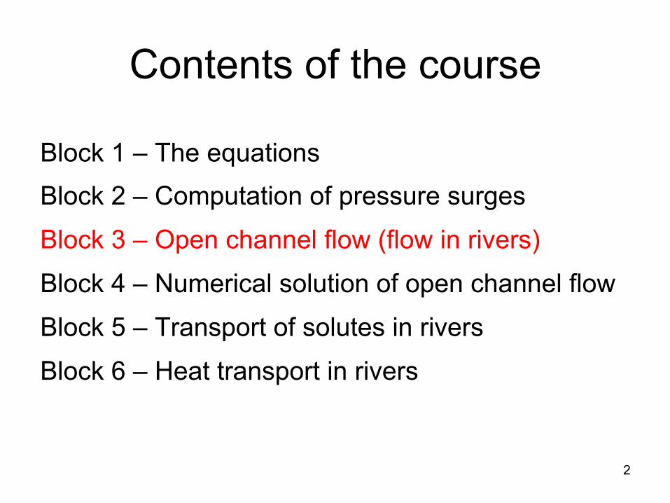
Contents of the course

Block 1 – The equations Block 2 – Computation of pressure surges

Block 3 – Open channel flow (flow in rivers)

Block 4 – Numerical solution of open channel flow

Block 5 – Transport of solutes in rivers

Block 6 – Heat transport in rivers

2

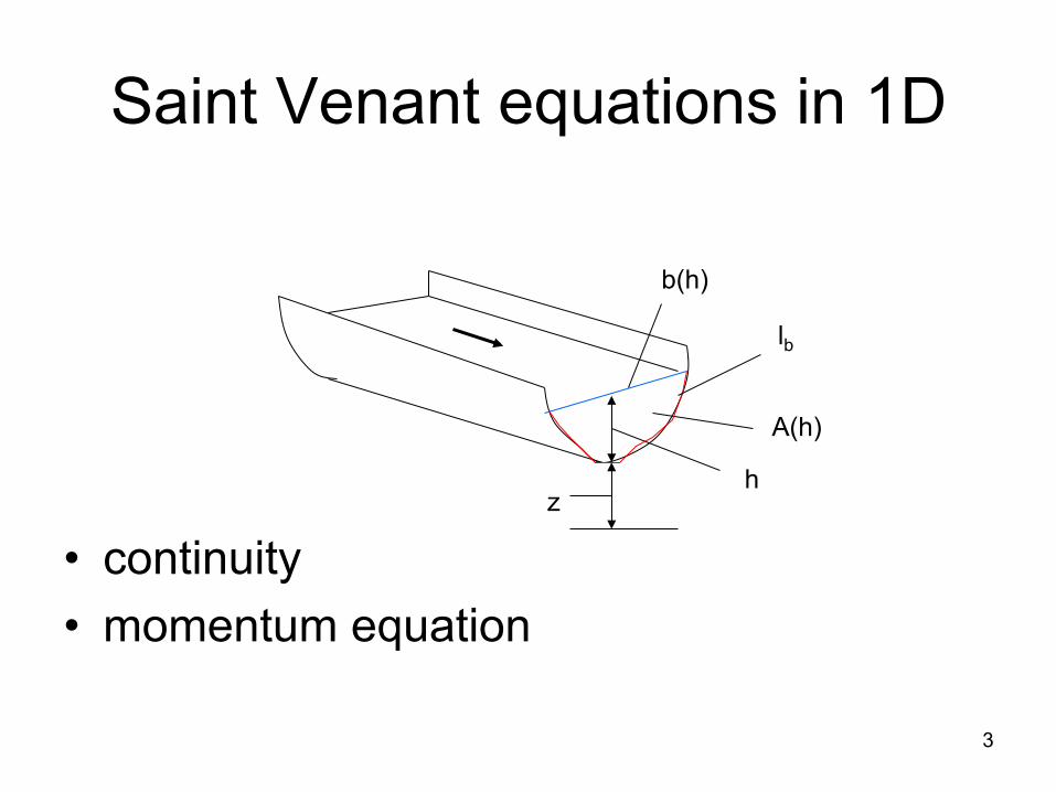
Saint Venant equations in 1D

•  continuity •  momentum equation

A(h)

h z

lb

b(h)

3

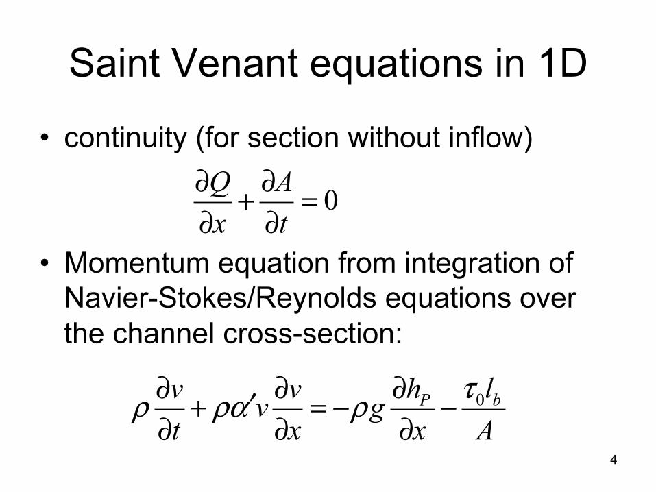
Saint Venant equations in 1D

•  continuity (for section without inflow)

•  Momentum equation from integration of Navier-Stokes/Reynolds equations over the channel cross-section:

0Q Ax t

∂ ∂+ =∂ ∂

0 bP lhv vv gt x x A

τρ ρα ρ ∂∂ ∂′+ = − −∂ ∂ ∂

4

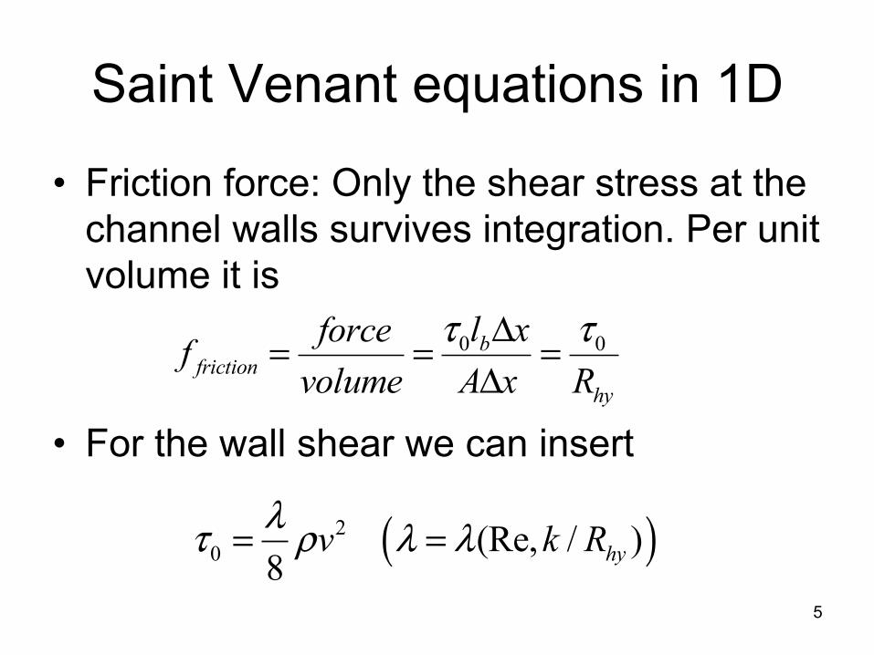
Saint Venant equations in 1D

•  Friction force: Only the shear stress at the channel walls survives integration. Per unit volume it is

•  For the wall shear we can insert

( )20 (Re, / )8 hyv k Rλτ ρ λ λ= =

0 0bfriction

hy

l xforcefvolume A x R

τ τΔ= = =Δ

5

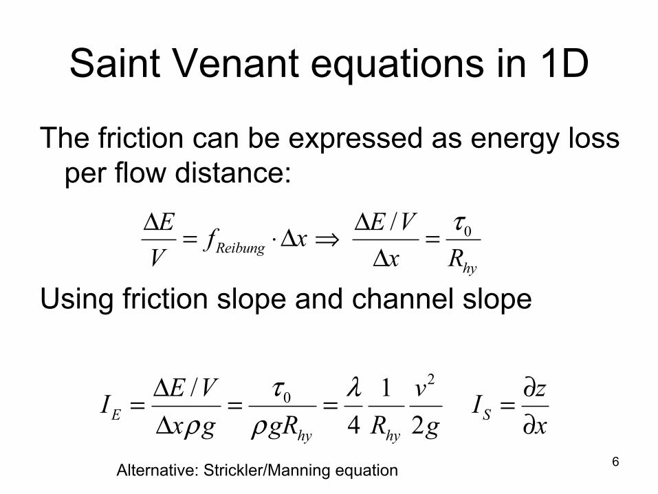
Saint Venant equations in 1D

The friction can be expressed as energy loss per flow distance:

Using friction slope and channel slope

0/Reibung

hy

E E Vf xV x R

τΔ Δ= ⋅Δ ⇒ =Δ

20/ 1

4 2E Shy hy

E V v zI Ix g gR R g x

τ λρ ρ

Δ ∂= = = =Δ ∂

Alternative: Strickler/Manning equation 6

Saint Venant equations in 1D

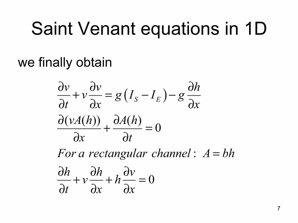
we finally obtain

( )( ( )) ( ) 0

:

0

S Ev v hv g I I gt x xvA h A hx t

For a rectangular channel A bhh h vv ht x x

∂ ∂ ∂+ = − −∂ ∂ ∂∂ ∂+ =

∂ ∂=

∂ ∂ ∂+ + =∂ ∂ ∂

7

Approximations and solutions

•  Steady state solution •  Kinematic wave •  Diffusive wave •  Full equations

8

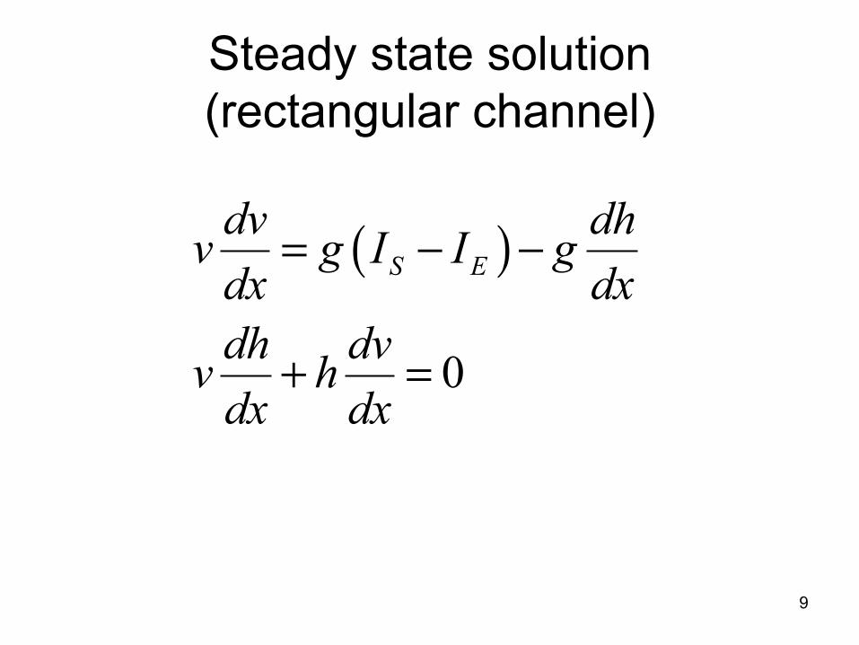
Steady state solution (rectangular channel)

( )

0

S Edv dhv g I I gdx dxdh dvv hdx dx

= − −

+ =

9

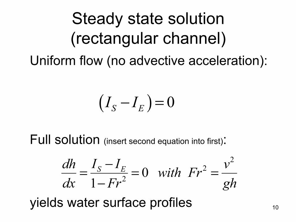
Steady state solution (rectangular channel)

( ) 0S EI I− =

Uniform flow (no advective acceleration): Full solution (insert second equation into first): yields water surface profiles

22

2 01S EI Idh vwith Fr

dx Fr gh−= = =

−10

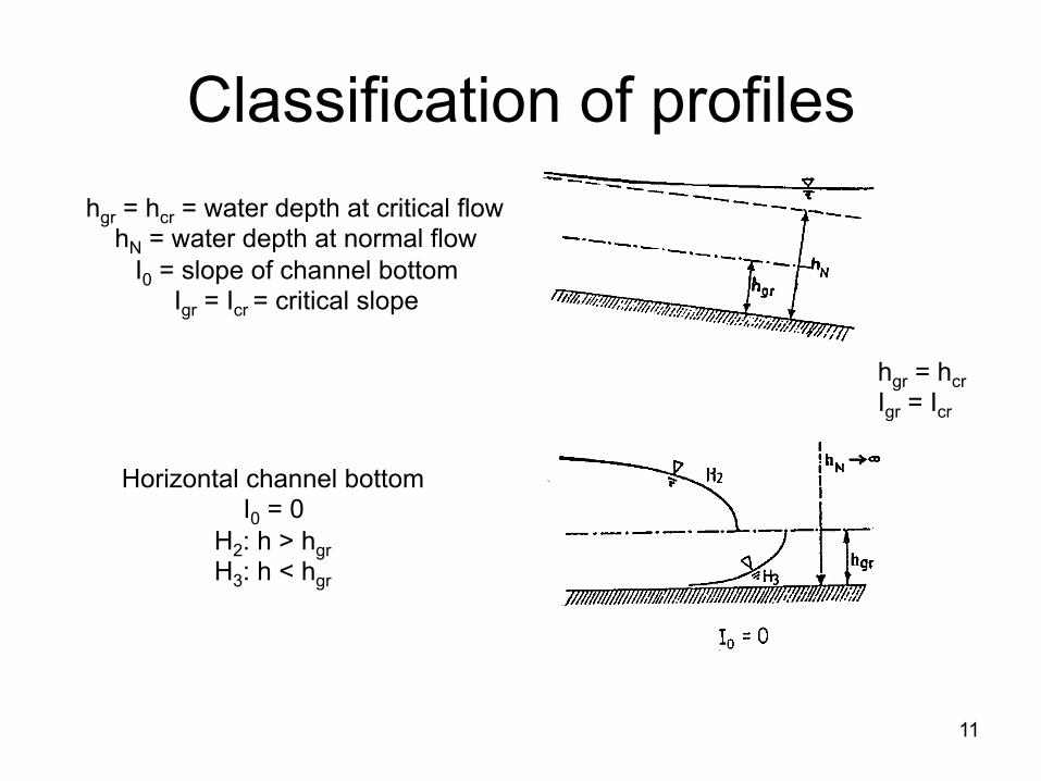
Classification of profiles hgr = hcr = water depth at critical flow

hN = water depth at normal flow I0 = slope of channel bottom

Igr = Icr = critical slope

Horizontal channel bottom I0 = 0

H2: h > hgr H3: h < hgr

hgr = hcr Igr = Icr

11

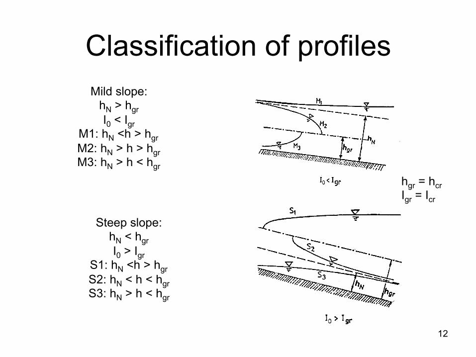
Classification of profiles Mild slope:

hN > hgr I0 < Igr

M1: hN <h > hgr M2: hN > h > hgr M3: hN > h < hgr

Steep slope: hN < hgr I0 > Igr

S1: hN <h > hgr S2: hN < h < hgr S3: hN > h < hgr

hgr = hcr Igr = Icr

12

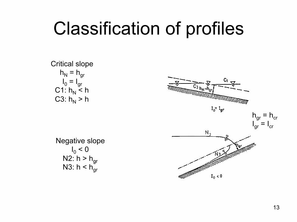
Classification of profiles

Critical slope hN = hgr I0 = Igr

C1: hN < h C3: hN > h

Negative slope I0 < 0

N2: h > hgr N3: h < hgr

hgr = hcr Igr = Icr

13

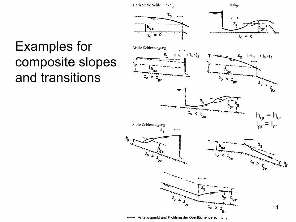
Examples for composite slopes and transitions

hgr = hcr Igr = Icr

14

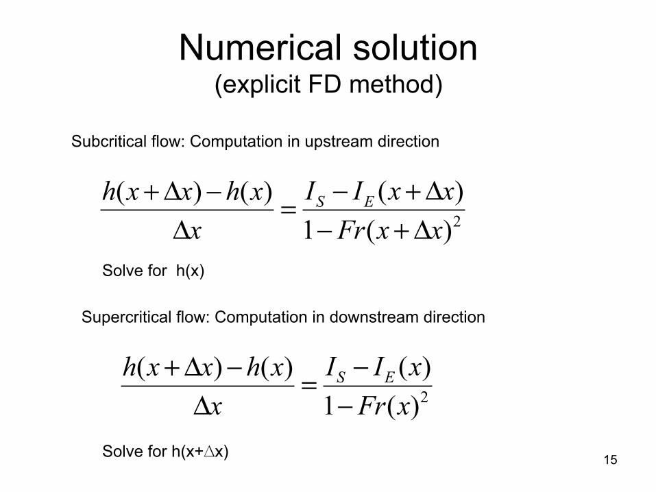
Numerical solution (explicit FD method)

2

( )( ) ( ) 01 ( )S EI I x xh x x h x

x Fr x x− +Δ+Δ − = =

Δ − +Δ

Subcritical flow: Computation in upstream direction

Supercritical flow: Computation in downstream direction

2

( )( ) ( ) 01 ( )S EI I xh x x h x

x Fr x−+Δ − = =

Δ −

Solve for h(x)

Solve for h(x+∆x) 15

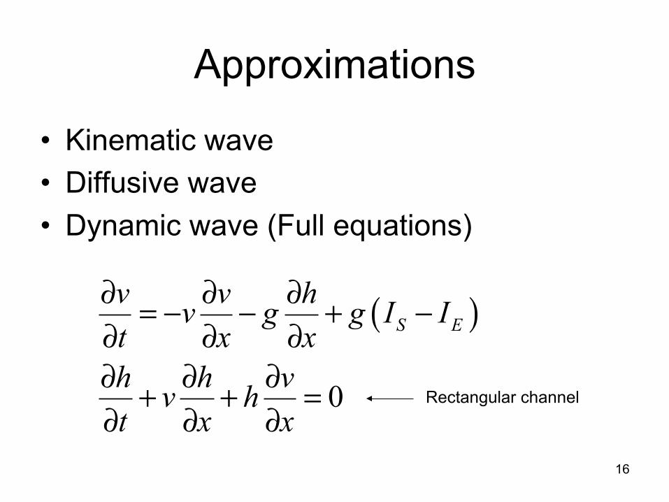
Approximations

•  Kinematic wave •  Diffusive wave •  Dynamic wave (Full equations)

( )

0

S Ev v hv g g I It x xh h vv ht x x

∂ ∂ ∂= − − + −∂ ∂ ∂∂ ∂ ∂+ + =∂ ∂ ∂

Rectangular channel

16

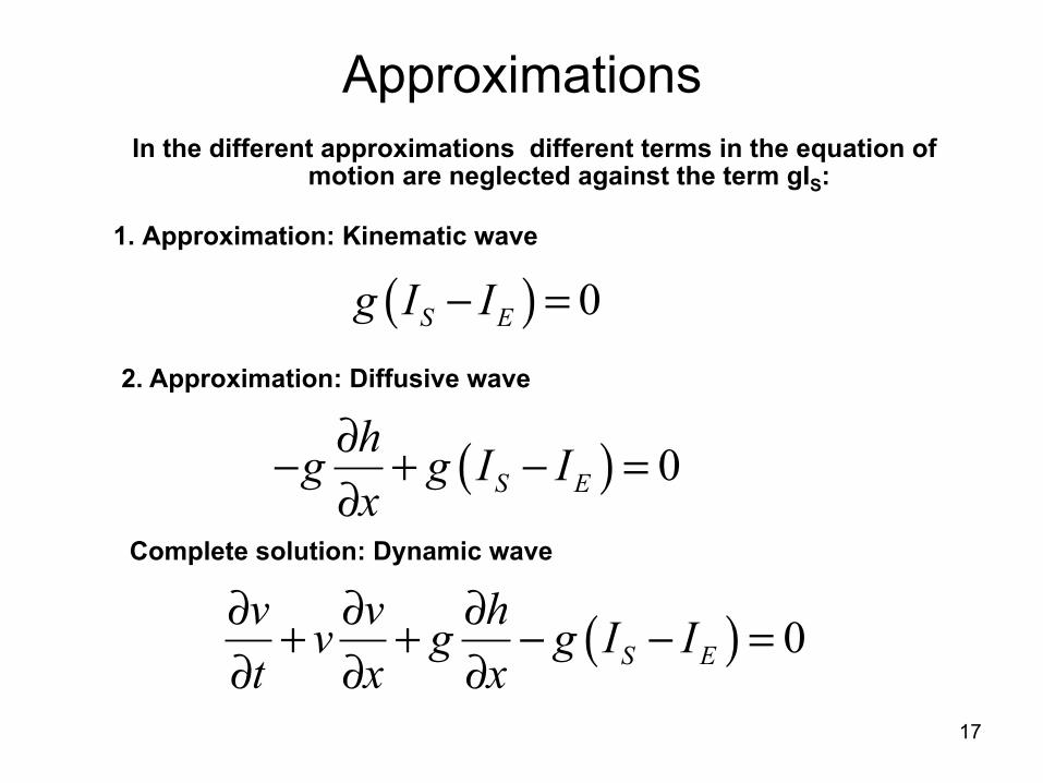
Approximations

1. Approximation: Kinematic wave

( ) 0S Ev v hv g g I It x x

∂ ∂ ∂+ + − − =∂ ∂ ∂

2. Approximation: Diffusive wave

Complete solution: Dynamic wave

( ) 0S Ehg g I Ix∂− + − =∂

( ) 0S Eg I I− =

In the different approximations different terms in the equation of motion are neglected against the term gIS:

17

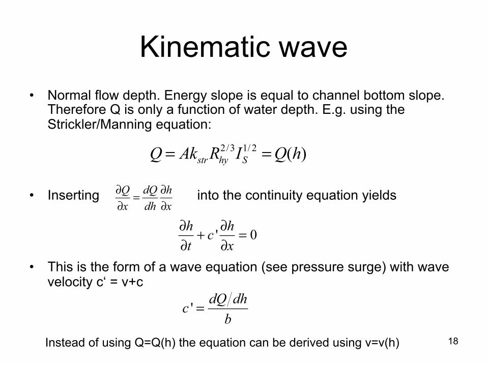
Kinematic wave •  Normal flow depth. Energy slope is equal to channel bottom slope.

Therefore Q is only a function of water depth. E.g. using the Strickler/Manning equation:

•  Inserting into the continuity equation yields

•  This is the form of a wave equation (see pressure surge) with wave velocity c‘ = v+c

2/3 1/ 2 ( )str hy SQ Ak R I Q h= =

Q dQ hx dh x

∂ ∂=∂ ∂

' 0h hct x

∂ ∂+ =∂ ∂

' dQ dhcb

=

Instead of using Q=Q(h) the equation can be derived using v=v(h) 18

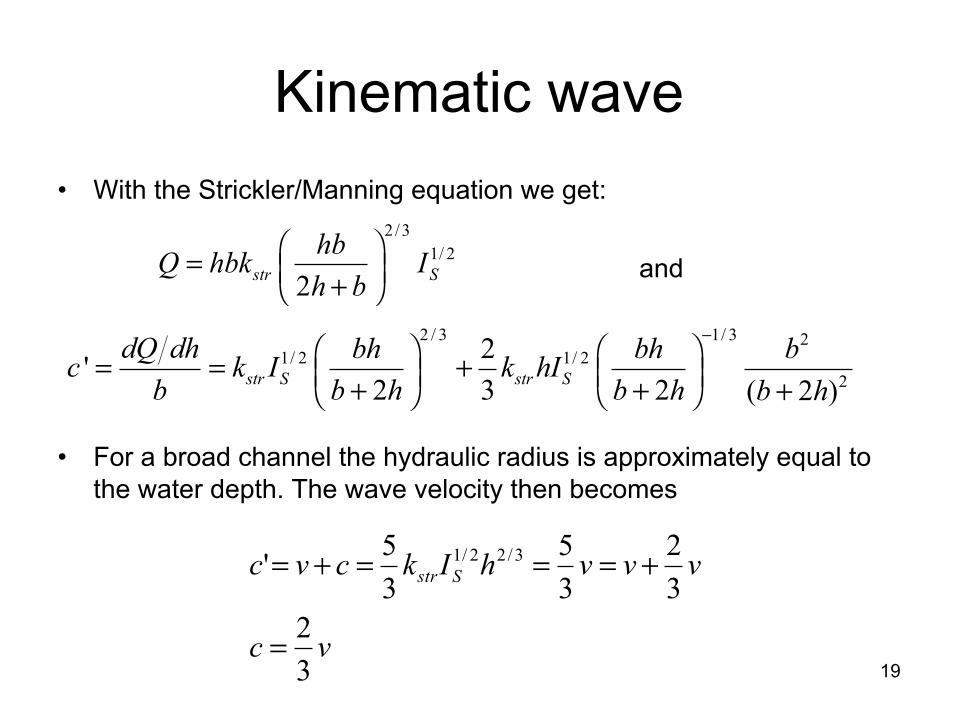
Kinematic wave •  With the Strickler/Manning equation we get:

•  For a broad channel the hydraulic radius is approximately equal to the water depth. The wave velocity then becomes

2/31/ 2

2str ShbQ hbk Ih b

⎛ ⎞= ⎜ ⎟+⎝ ⎠2 / 3 1/ 3 2

1/ 2 1/ 22

2'2 3 2 ( 2 )str S str S

dQ dh bh bh bc k I k hIb b h b h b h

−⎛ ⎞ ⎛ ⎞= = +⎜ ⎟ ⎜ ⎟+ + +⎝ ⎠ ⎝ ⎠

and

vc

vvvhIkcvc Sstr

32

32

35

35' 3/22/1

=

+===+=

19

Kinematic wave •  The wave velocity is not constant as v is a

function of water depth h. •  Varying velocities for different water depth lead

to self-sharpening of wave front •  Pressure propagates faster than the average

flow. •  Advantage of approximation: PDE of first

order, only one upstream boundary condition required.

•  Disadvantage of approximation: Not applicable for bottom slope 0. No backwater feasible as there is no downstream boundary condition.

20

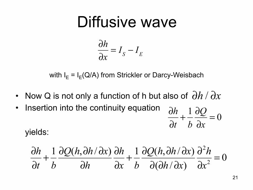
Diffusive wave

•  Now Q is not only a function of h but also of •  Insertion into the continuity equation

yields:

∂h∂x

= IS − IE

with IE = IE(Q/A) from Strickler or Darcy-Weisbach

1 0h Qt b x

∂ ∂+ =∂ ∂

2

2

1 ( , / ) 1 ( , / ) 0( / )

h Q h h x h Q h h x ht b h x b h x x

∂ ∂ ∂ ∂ ∂ ∂ ∂ ∂ ∂+ + =∂ ∂ ∂ ∂ ∂ ∂ ∂

21

∂h / ∂x

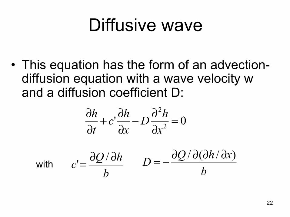
Diffusive wave

•  This equation has the form of an advection-diffusion equation with a wave velocity w and a diffusion coefficient D:

with

0' 2

2

=∂∂−

∂∂+

∂∂

xhD

xhc

th

bhQc ∂∂= /' b

xhQD )/(/ ∂∂∂∂−=

22

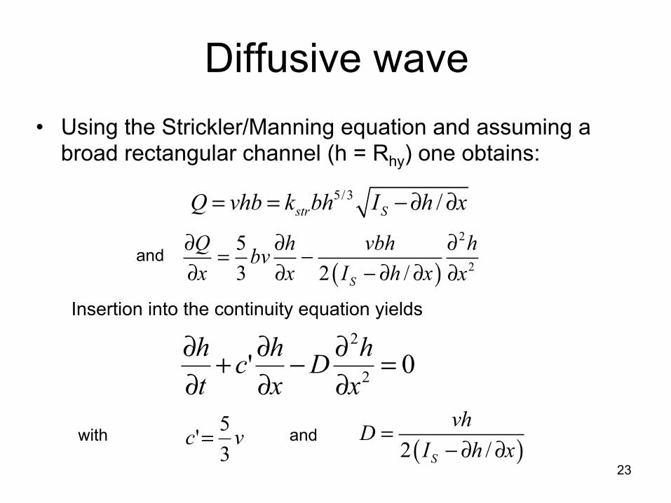
Diffusive wave •  Using the Strickler/Manning equation and assuming a

broad rectangular channel (h = Rhy) one obtains:

5/3 /str SQ vhb k bh I h x= = −∂ ∂

and

Insertion into the continuity equation yields

with and

0' 2

2

=∂∂−

∂∂+

∂∂

xhD

xhc

th

vc35'= ( )2 /S

vhDI h x

=− ∂ ∂

( )2

2

53 2 /S

Q h vbh hbvx x I h x x

∂ ∂ ∂= −∂ ∂ − ∂ ∂ ∂

23

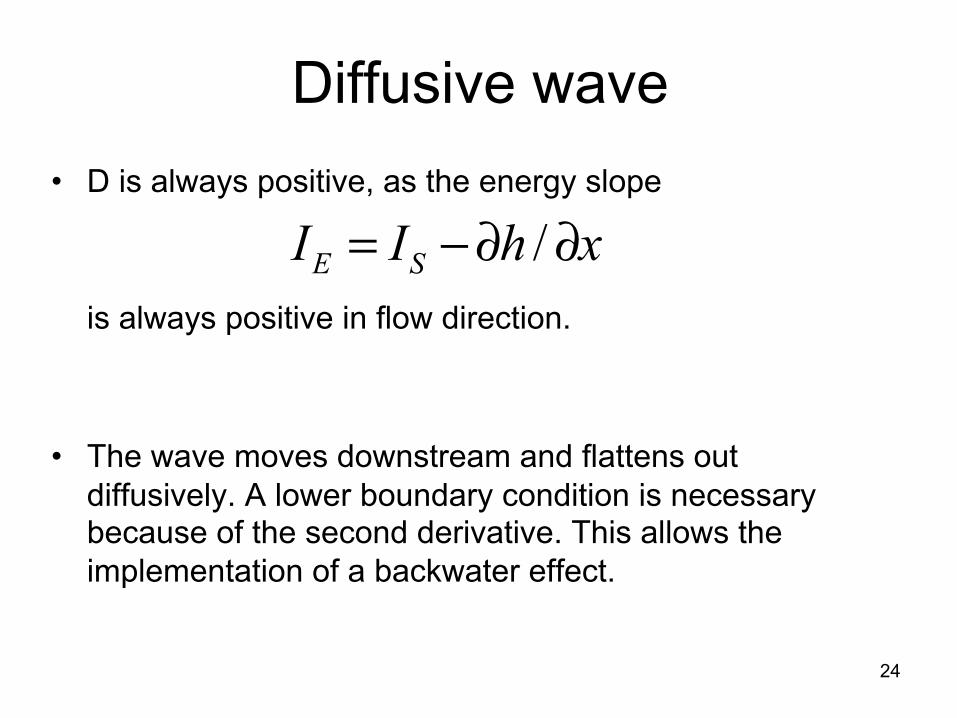
Diffusive wave •  D is always positive, as the energy slope

is always positive in flow direction.

•  The wave moves downstream and flattens out

diffusively. A lower boundary condition is necessary because of the second derivative. This allows the implementation of a backwater effect.

/E SI I h x= −∂ ∂

24

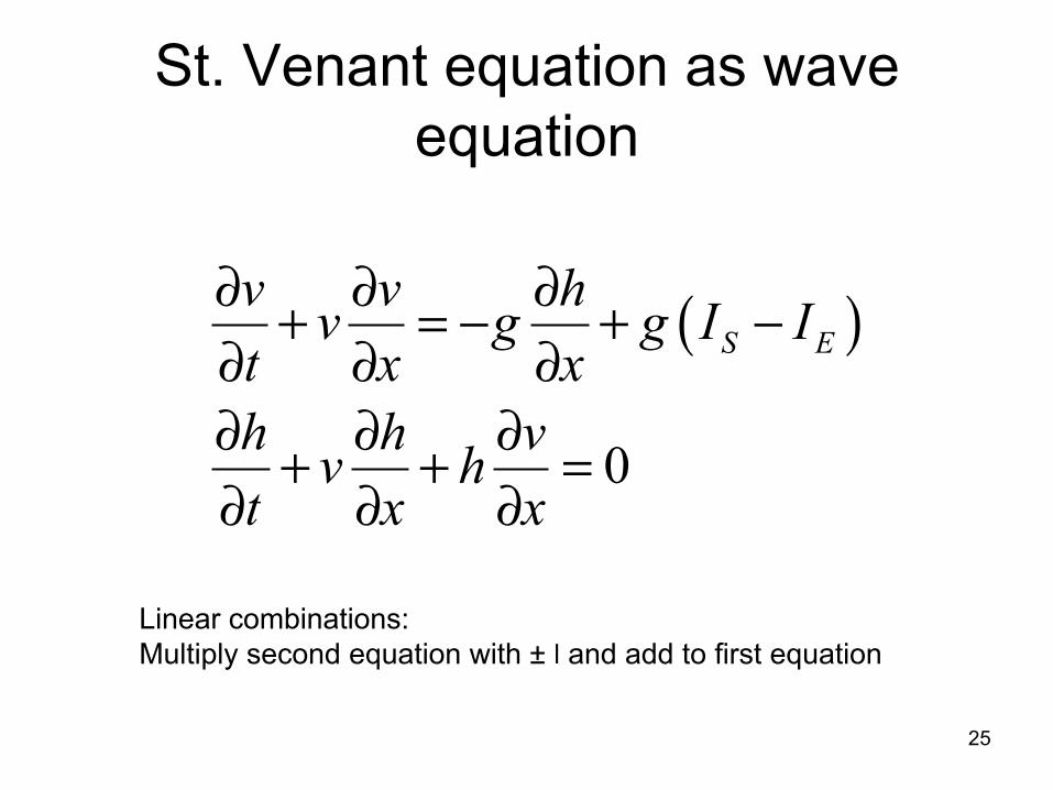
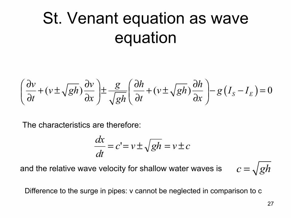
St. Venant equation as wave equation

( )

0

S Ev v hv g g I It x xh h vv ht x x

∂ ∂ ∂+ = − + −∂ ∂ ∂∂ ∂ ∂+ + =∂ ∂ ∂

Linear combinations: Multiply second equation with ± l and add to first equation

25

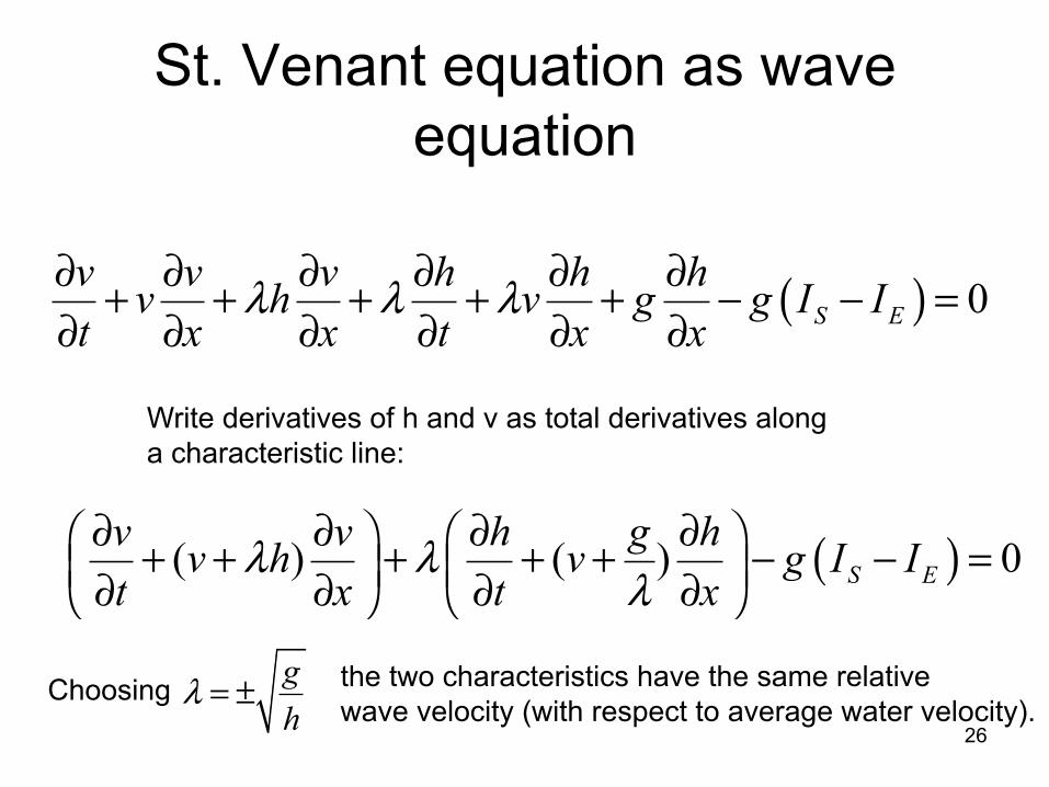
St. Venant equation as wave equation

( ) 0S Ev v v h h hv h v g g I It x x t x x

λ λ λ∂ ∂ ∂ ∂ ∂ ∂+ + + + + − − =∂ ∂ ∂ ∂ ∂ ∂

Write derivatives of h and v as total derivatives along a characteristic line:

( )( ) ( ) 0S Ev v h g hv h v g I It x t x

λ λλ

∂ ∂ ∂ ∂⎛ ⎞ ⎛ ⎞+ + + + + − − =⎜ ⎟ ⎜ ⎟∂ ∂ ∂ ∂⎝ ⎠ ⎝ ⎠

Choosing gh

λ = ± the two characteristics have the same relative wave velocity (with respect to average water velocity).

26

St. Venant equation as wave equation

( )( ) ( ) 0S Ev v g h hv gh v gh g I It x t xgh

∂ ∂ ∂ ∂⎛ ⎞ ⎛ ⎞+ ± ± + ± − − =⎜ ⎟ ⎜ ⎟∂ ∂ ∂ ∂⎝ ⎠ ⎝ ⎠

and the relative wave velocity for shallow water waves is c gh=

The characteristics are therefore:

Difference to the surge in pipes: v cannot be neglected in comparison to c

cvghvcdtdx ±=±== '

27

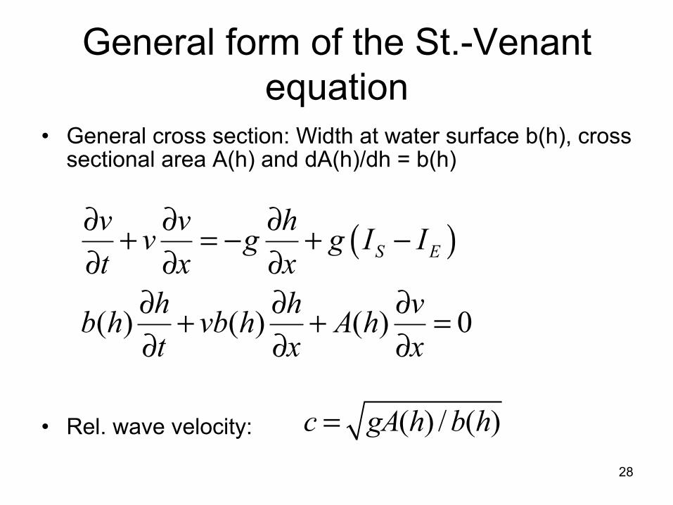
General form of the St.-Venant equation

•  General cross section: Width at water surface b(h), cross sectional area A(h) and dA(h)/dh = b(h)

•  Rel. wave velocity:

( )

( ) ( ) ( ) 0

S Ev v hv g g I It x x

h h vb h vb h A ht x x

∂ ∂ ∂+ = − + −∂ ∂ ∂

∂ ∂ ∂+ + =∂ ∂ ∂

( ) / ( )c gA h b h=28

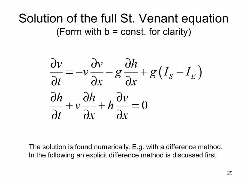
Solution of the full St. Venant equation (Form with b = const. for clarity)

( )

0

S Ev v hv g g I It x xh h vv ht x x

∂ ∂ ∂= − − + −∂ ∂ ∂∂ ∂ ∂+ + =∂ ∂ ∂

The solution is found numerically. E.g. with a difference method. In the following an explicit difference method is discussed first.

29