BMÜ-357 SAYISAL GÖRÜNTÜ İŞLEME

MATLAB UYGULAMALARIYrd. Doç. Dr. İlhan AYDIN

Örnek-1

• imfinfo(‘cameraman.tif ’)

• I1=imread(‘cameraman.tif ’);

• imwrite(I1,’cameraman.jpg’,’jpg’);

• imfinfo(‘cameraman.jpg’)

A=imread(‘cameraman.tif ’);

imshow(A);

imagesc(A);

axis image;

axis off;

colormap(gray);

Örnek:

B=rand(256).1000;

imshow(B);

imagesc(B);

axis image;

axis off;

colormap(gray);

colorbar;

imshow(B,[0 1000]);

Örnek:

B=imread('cell.tif');

C=imread('spine.tif');

D=imread('onion.png');

subplot(3,1,1); imagesc(B); axis image;

axis off; colormap(gray);

subplot(3,1,2); imagesc(C); axis image; axis off;

colormap(jet);

subplot(3,1,3); imshow(D);

Örnek:

B=imread('cell.tif'); % Read in 8-bit intensity image of cell

imtool(B); % examine grayscale image in interactive

viewer

D=imread('onion.png'); % Read in 8-bit colour image.

imtool(D); % examine RGB image in interactive viewer

B(25,50) % print pixel value at location (25,50)

B(25,50) = 255; % set pixel value at (25,50) to white

imshow(B); % view resulting changes in image

D(25,50, :) % print RGB pixel value at location

(25,50)

D(25,50, 1) % print only the red value at (25,50)

D(25,50,:)=[255,255, 255]; % set pixel value to RGB white

imshow(D); % view resulting changes in image

Örnek:

D=imread('onion.png'); % Read in 8-bit RGB colour image.

Dgray = rgb2gray(D); % convert it to a grayscale image

subplot(2,1,1); imshow(D);

axis image; % display both side by side

subplot(2,1,2); imshow(Dgray);

Örnek:

A=imread('cameraman.tif'); % Read in image

subplot(1,2,1), imshow(A); % Display image

B = imadd(A, 100); % Add 100 pixel values to image A

subplot(1,2,2), imshow(B); % Display result image B

Örnek:

A=imread('cameraman.tif');

subplot(1,2,1), imshow(A);

B = imcomplement(A);

subplot(1,2,2), imshow(B);

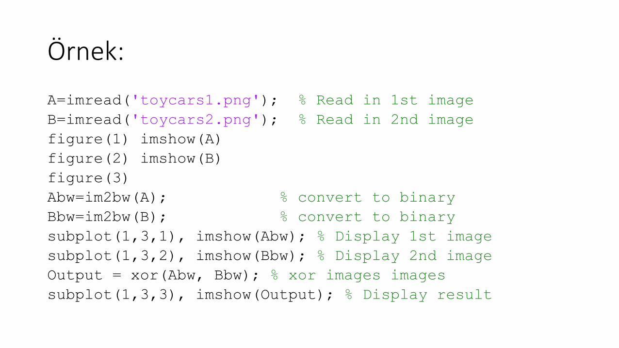
Örnek:

A=imread('toycars1.png'); % Read in 1st image

B=imread('toycars2.png'); % Read in 2nd image

figure(1) imshow(A)

figure(2) imshow(B)

figure(3)

Abw=im2bw(A); % convert to binary

Bbw=im2bw(B); % convert to binary

subplot(1,3,1), imshow(Abw); % Display 1st image

subplot(1,3,2), imshow(Bbw); % Display 2nd image

Output = xor(Abw, Bbw); % xor images images

subplot(1,3,3), imshow(Output); % Display result

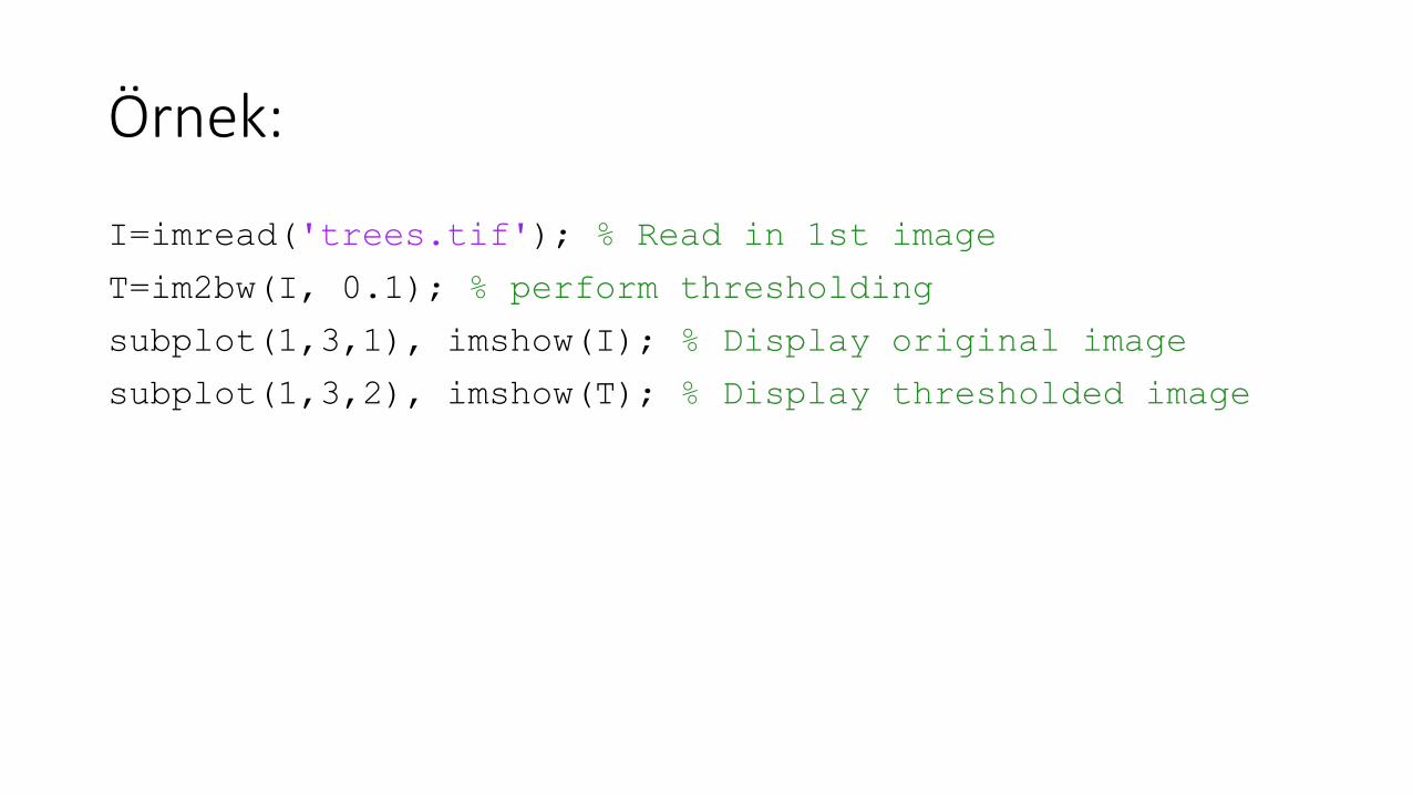
Örnek:

I=imread('trees.tif'); % Read in 1st image

T=im2bw(I, 0.1); % perform thresholding

subplot(1,3,1), imshow(I); % Display original image

subplot(1,3,2), imshow(T); % Display thresholded image

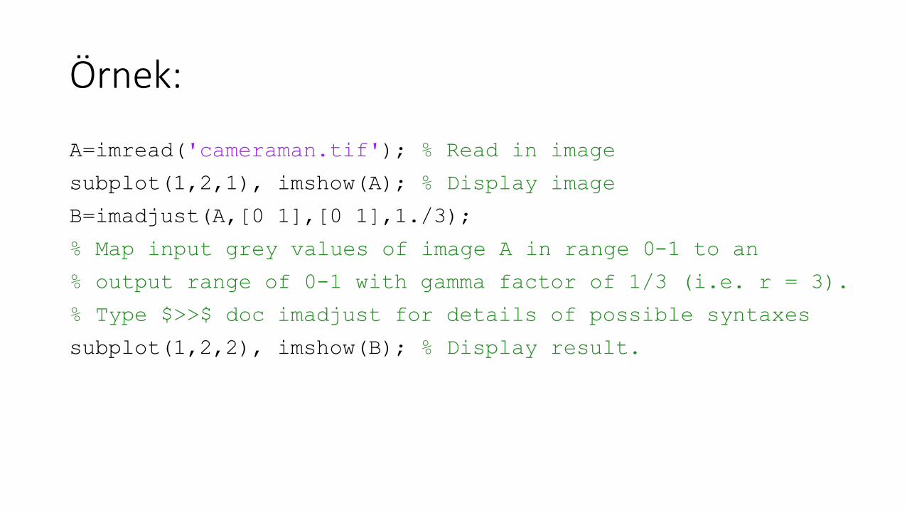
Örnek:

A=imread('cameraman.tif'); % Read in image

subplot(1,2,1), imshow(A); % Display image

B=imadjust(A,[0 1],[0 1],1./3);

% Map input grey values of image A in range 0-1 to an

% output range of 0-1 with gamma factor of 1/3 (i.e. r = 3).

% Type $>>$ doc imadjust for details of possible syntaxes

subplot(1,2,2), imshow(B); % Display result.

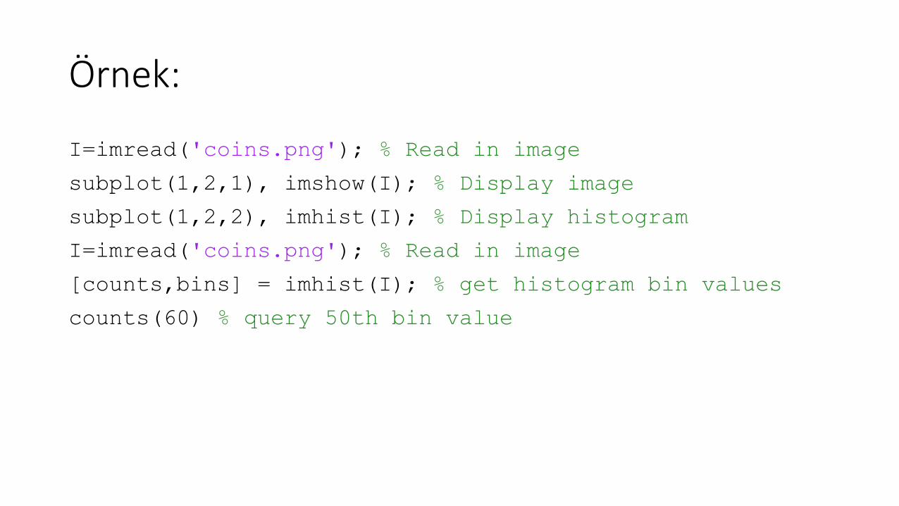
Örnek:

I=imread('coins.png'); % Read in image

subplot(1,2,1), imshow(I); % Display image

subplot(1,2,2), imhist(I); % Display histogram

I=imread('coins.png'); % Read in image

[counts,bins] = imhist(I); % get histogram bin values

counts(60) % query 50th bin value

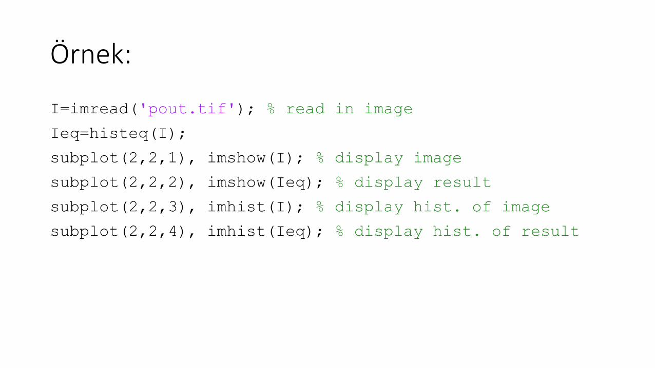
Örnek:

I=imread('pout.tif'); % read in image

Ieq=histeq(I);

subplot(2,2,1), imshow(I); % display image

subplot(2,2,2), imshow(Ieq); % display result

subplot(2,2,3), imhist(I); % display hist. of image

subplot(2,2,4), imhist(Ieq); % display hist. of result

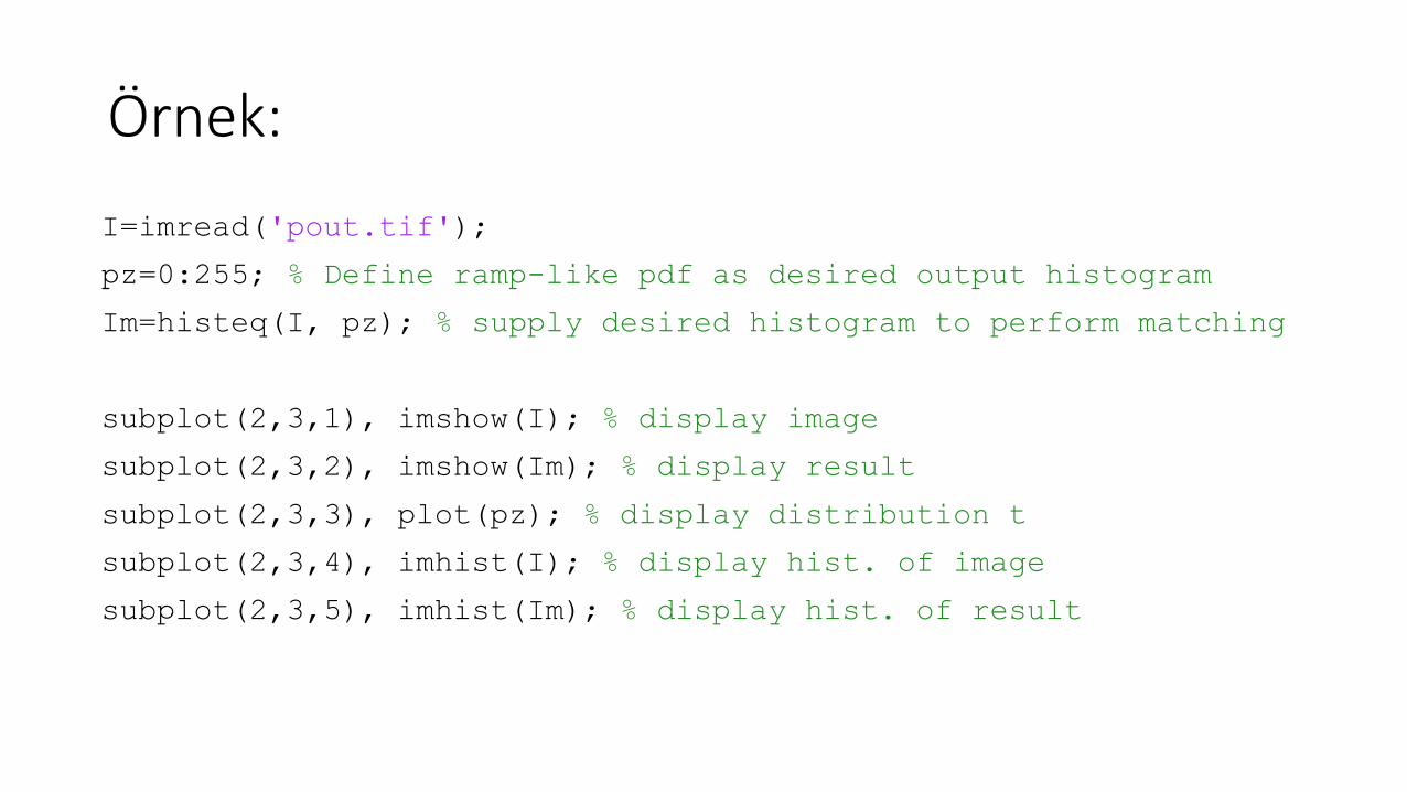
Örnek:

I=imread('pout.tif');

pz=0:255; % Define ramp-like pdf as desired output histogram

Im=histeq(I, pz); % supply desired histogram to perform matching

subplot(2,3,1), imshow(I); % display image

subplot(2,3,2), imshow(Im); % display result

subplot(2,3,3), plot(pz); % display distribution t

subplot(2,3,4), imhist(I); % display hist. of image

subplot(2,3,5), imhist(Im); % display hist. of result

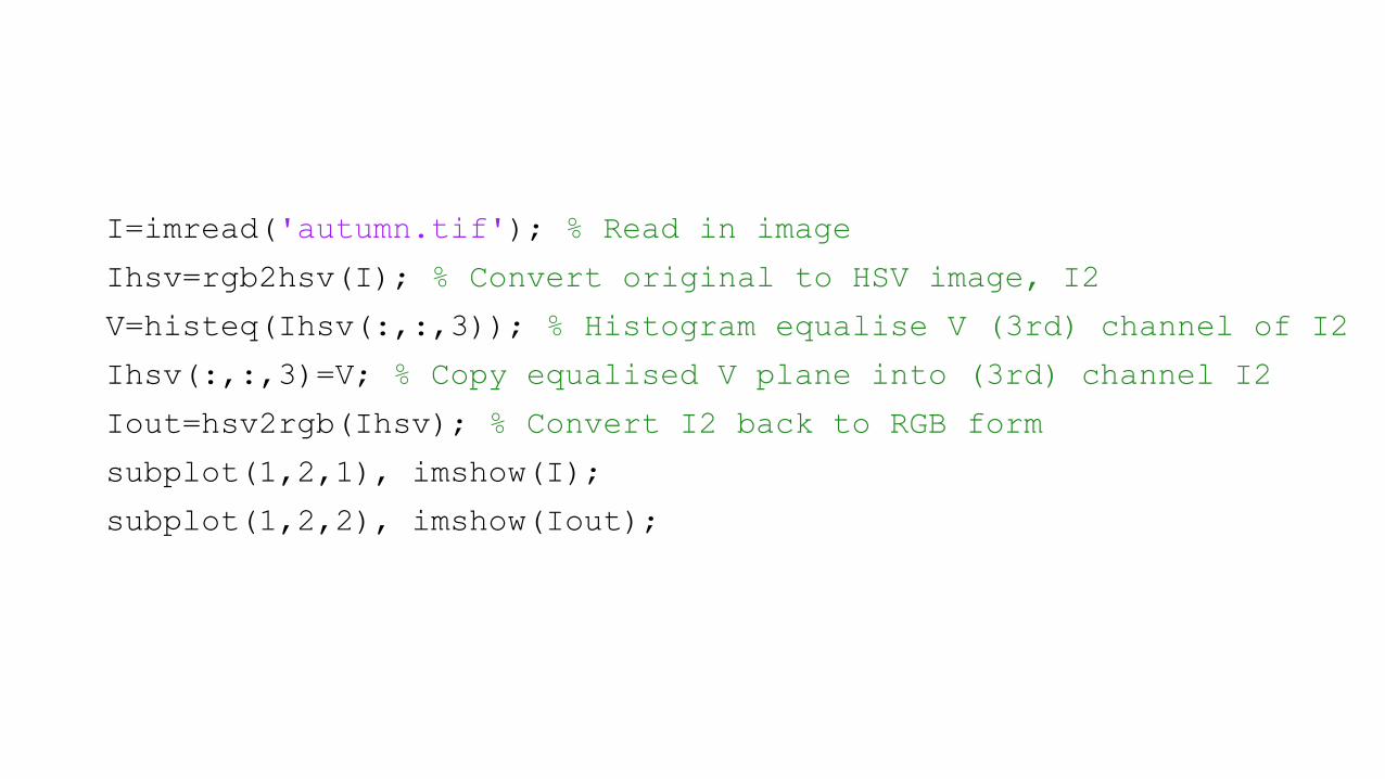
I=imread('autumn.tif'); % Read in image

Ihsv=rgb2hsv(I); % Convert original to HSV image, I2

V=histeq(Ihsv(:,:,3)); % Histogram equalise V (3rd) channel of I2

Ihsv(:,:,3)=V; % Copy equalised V plane into (3rd) channel I2

Iout=hsv2rgb(Ihsv); % Convert I2 back to RGB form

subplot(1,2,1), imshow(I);

subplot(1,2,2), imshow(Iout);

Örnek:

A=imread('peppers.png'); % Read in image

subplot(1,2,1), imshow(A); % Display image

k = fspecial('motion', 50, 54); % create a 5x5 convolution kernel

B = imfilter(A, k, 'symmetric'); % apply using symmetric mirroring at edges

subplot(1,2,2), imshow(B); % Display result image B

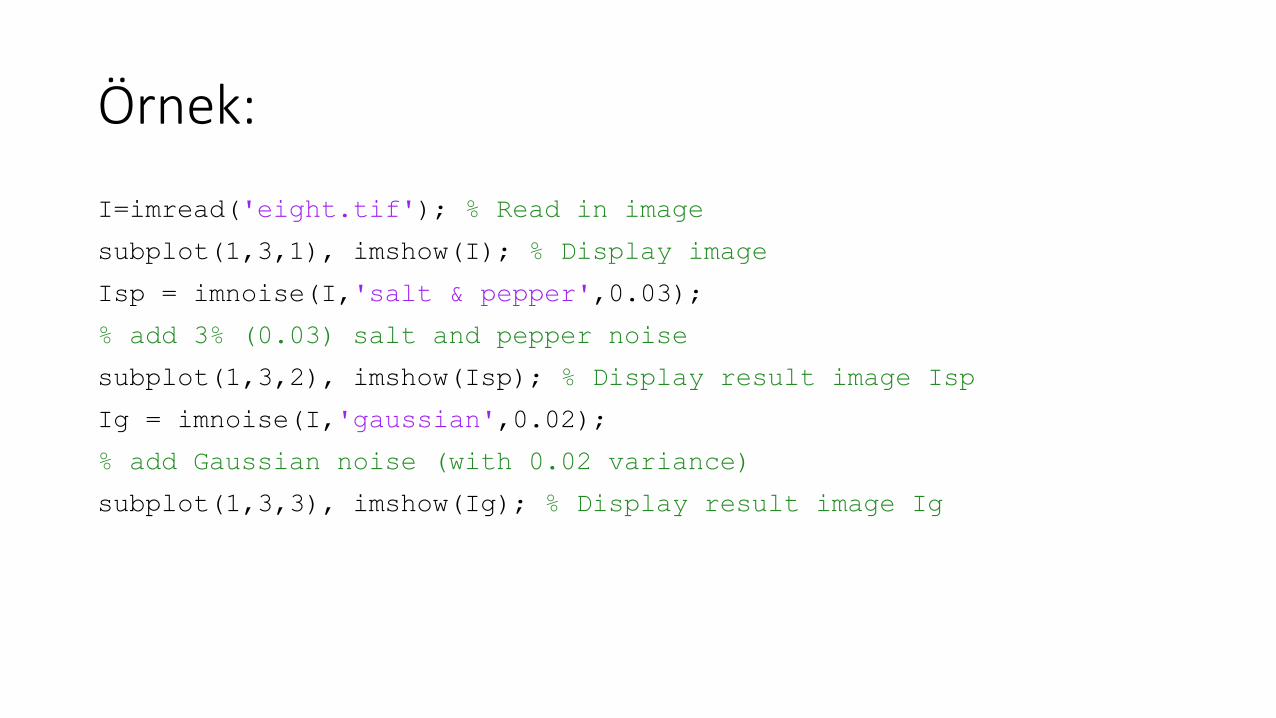
Örnek:

I=imread('eight.tif'); % Read in image

subplot(1,3,1), imshow(I); % Display image

Isp = imnoise(I,'salt & pepper',0.03);

% add 3% (0.03) salt and pepper noise

subplot(1,3,2), imshow(Isp); % Display result image Isp

Ig = imnoise(I,'gaussian',0.02);

% add Gaussian noise (with 0.02 variance)

subplot(1,3,3), imshow(Ig); % Display result image Ig

Örnek devamk = ones(3,3) / 9; % define mean filter

I_m = imfilter(I,k); % apply to original image

Isp_m = imfilter(Isp,k); % apply to salt and pepper image

Ig_m = imfilter(Ig,k); % apply tp gaussian image

subplot(1,3,1), imshow(I_m); % Display result image

subplot(1,3,2), imshow(Isp_m); % Display result image

subplot(1,3,3), imshow(Ig_m); % Display result image

I_m = medfilt2(I,[3 3]); % apply to original image

Isp_m = medfilt2(Isp,[3 3]); % apply to salt and pepper image

Ig_m =medfilt2(Ig,[3 3]); % apply tp gaussian image

subplot(1,3,1), imshow(I_m); % Display result image

subplot(1,3,2), imshow(Isp_m); % Display result image

subplot(1,3,3), imshow(Ig_m); % Display result image

Örnek: function fftshow(f,type)

if nargin<2

type='log';

end

if(type=='log')

f1=log(1+abs(f));

fm=max(f1(:));

imshow(im2uint8(f1/fm));

elseif (type=='abs')

fa=abs(f);

fm=max(fa(:));

imshow(fa/fm);

else

error('Hatalý secim')

end

>>A=imread('cameraman.tif');>> cf=fftshift(fft2(A));>> fftshow(cf,'log')

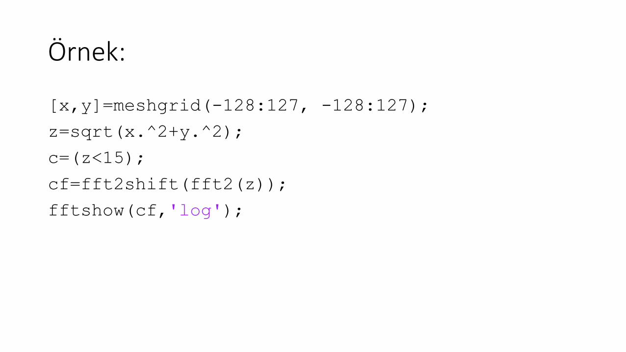
Örnek:

[x,y]=meshgrid(-128:127, -128:127);

z=sqrt(x.^2+y.^2);

c=(z<15);

cf=fft2shift(fft2(z));

fftshow(cf,'log');

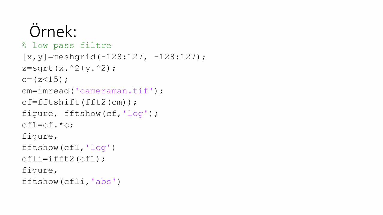
Örnek: % low pass filtre

[x,y]=meshgrid(-128:127, -128:127);

z=sqrt(x.^2+y.^2);

c=(z<15);

cm=imread('cameraman.tif');

cf=fftshift(fft2(cm));

figure, fftshow(cf,'log');

cf1=cf.*c;

figure,

fftshow(cf1,'log')

cfli=ifft2(cf1);

figure,

fftshow(cfli,'abs')