Embed Size (px)
Citation preview

BVP of ODE 1
Boundary-Value Problems for Ordinary
Differential Equations
NTNU
Tsung-Min Hwang
December 20, 2003
Department of Mathematics – NTNU Tsung-Min Hwang December 20, 2003

BVP of ODE 2
1 – Mathematical Theories . . . . . . . . . . . . . . . . . . . . . . . . . . . . . 4
2 – Finite Difference Method For Linear Problems . . . . . . . . . . . . . . . . . 15
2.1 – The Finite Difference Formulation . . . . . . . . . . . . . . . . . . . . . . 15
2.2 – Convergence Analysis . . . . . . . . . . . . . . . . . . . . . . . . . . . 19
3 – Shooting Methods . . . . . . . . . . . . . . . . . . . . . . . . . . . . . . . 22
Department of Mathematics – NTNU Tsung-Min Hwang December 20, 2003

BVP of ODE 3
The two-point boundary-value problems (BVP) considered in this chapter involve a
second-order differential equation together with boundary condition in the following form:
y′′ = f(x, y, y′)
y(a) = α, y(b) = β(1)
The numerical procedures for finding approximate solutions to the initial-value problems can
not be adapted to the solution of this problem since the specification of conditions involve
two different points, x = a and x = b. New techniques are introduced in this chapter for
handling problems (1) in which the conditions imposed are of a boundary-value rather than
an initial-value type.
Department of Mathematics – NTNU Tsung-Min Hwang December 20, 2003

BVP of ODE 3
The two-point boundary-value problems (BVP) considered in this chapter involve a
second-order differential equation together with boundary condition in the following form:
y′′ = f(x, y, y′)
y(a) = α, y(b) = β(1)
The numerical procedures for finding approximate solutions to the initial-value problems can
not be adapted to the solution of this problem since the specification of conditions involve
two different points, x = a and x = b.
New techniques are introduced in this chapter for
handling problems (1) in which the conditions imposed are of a boundary-value rather than
an initial-value type.
Department of Mathematics – NTNU Tsung-Min Hwang December 20, 2003

BVP of ODE 3
The two-point boundary-value problems (BVP) considered in this chapter involve a
second-order differential equation together with boundary condition in the following form:
y′′ = f(x, y, y′)
y(a) = α, y(b) = β(1)
The numerical procedures for finding approximate solutions to the initial-value problems can
not be adapted to the solution of this problem since the specification of conditions involve
two different points, x = a and x = b. New techniques are introduced in this chapter for
handling problems (1) in which the conditions imposed are of a boundary-value rather than
an initial-value type.
Department of Mathematics – NTNU Tsung-Min Hwang December 20, 2003

BVP of ODE 4
1 – Mathematical Theories
Before considering numerical methods, a few mathematical theories about the two-point
boundary-value problem (1), such as the existence and uniqueness of solution, shall be
discussed in this section.
Theorem 1 Suppose that f in (1) is continuous on the set
D = {(x, y, y′)|a ≤ x ≤ b, −∞ < y < ∞, −∞ < y′ < ∞} ,
and that∂f
∂yand
∂f
∂y′are also continuous on D. If
1.∂f
∂y(x, y, y′) > 0 for all (x, y, y′) ∈ D, and
2. a constant M exists, with
∣
∣
∣
∣
∂f
∂y′(x, y, y′)
∣
∣
∣
∣
≤ M , ∀ (x, y, y′) ∈ D,
then (1) has a unique solution.
Department of Mathematics – NTNU Tsung-Min Hwang December 20, 2003

BVP of ODE 5
When the function f(x, y, y′) has the special form
f(x, y, y′) = p(x)y′ + q(x)y + r(x),
the differential equation become a so-called linear problem. The previous theorem can be
simplified for this case.
Corollary 1 If the linear two-point boundary-value problem
y′′ = p(x)y′ + q(x)y + r(x)
y(a) = α, y(b) = β
satisfies
1. p(x), q(x), and r(x) are continuous on [a, b], and
2. q(x) > 0 on [a, b],
then the problem has a unique solution.
Department of Mathematics – NTNU Tsung-Min Hwang December 20, 2003

BVP of ODE 6
Many theories and application models consider the boundary-value problem in a special
form as follows.
y′′ = f(x, y)
y(0) = 0, y(1) = 0
We will show that this simple form can be derived from the original problem by simple
techniques such as changes of variables and linear transformation. To do this, we begin by
changing the variable. Suppose that the original problem is
y′′ = f(x, y)
y(a) = α, y(b) = β(2)
where y = y(x). Now let λ = b − a and define a new variable
t =x − a
b − a=
1
λ(x − a).
Department of Mathematics – NTNU Tsung-Min Hwang December 20, 2003

BVP of ODE 7
That is, x = a + λt. Notice that t = 0 corresponds to x = a, and t = 1 corresponds to
x = b. Then we define
z(t) = y(a + λt) = y(x)
with λ = b − a. This gives
z′(t) =d
dtz(t) =
d
dty(a + λt) =
[
d
dxy(x)
] [
d
dt(a + λt)
]
= λy′(x)
and, analogously,
z′′(t) =d
dtz′(t) = λ2y′′(x) = λ2f(x, y(x)) = λ2f(a + λt, z(t)).
Likewise the boundary conditions are changed to
z(0) = y(a) = α and z(1) = y(b) = β.
Department of Mathematics – NTNU Tsung-Min Hwang December 20, 2003
BVP of ODE 8
With all these together, the problem (2) is transformed into
z′′(t) = λ2f(a + λt, z(t))
z(0) = α, z(1) = β(3)
Thus, if y(x) is a solution for (2), then z(t) = y(a + λt) is a solution for the
boundary-value problem (3). Conversely, if z(t) is a solution for (3), then
y(x) = z( 1λ(x − a)) is a solution for (2).
Example 1 Simplify the boundary conditions of the following equation by use of changing
variables.
y′′ = sin(xy) + y2
y(1) = 3, y(4) = 7
Solution: In this problem a = 1, b = 4, hence λ = 3. Now define the new variable
t = 13 (x − 1), hence x = 1 + 3t, and let z(t) = y(x) = y(1 + 3t). Then
Department of Mathematics – NTNU Tsung-Min Hwang December 20, 2003

BVP of ODE 9
λ2f(a + λt, z) = 9[
sin(1 + 3t)z + z2]
,
and the original equation is reduced to
z′′(t) = 9 sin((1 + 3t)z) + 9z2
z(0) = 3, z(1) = 7
To reduce a two-point boundary-value problem
z′′(t) = g(t, z)
z(0) = α, z(1) = β
to a homogeneous system, let
u(t) = z(t) − [α + (β − α)t]
then u′′(t) = z′′(t), and
u(0) = z(0) − α = 0 and u(1) = z(1) − β = 0
Department of Mathematics – NTNU Tsung-Min Hwang December 20, 2003

BVP of ODE 10
Moreover,
g(t, z) = g(t, u + α + (β − α)t) ≡ h(t, u).
The system is now transformed into
u′′(t) = h(t, u)
u(0) = 0, u(1) = 0
Example 2 Reduce the system
z′′ = [5z − 10t + 35 + sin(3z − 6t + 21)]et
z(0) = −7, z(1) = −5
to a homogeneous problem by linear transformation technique.
Solution: Let
u(t) = z(t) − [−7 + (−5 + 7)t] = z(t) − 2t + 7.
Department of Mathematics – NTNU Tsung-Min Hwang December 20, 2003

BVP of ODE 11
Then z(t) = u(t) + 2t − 7, and
u′′ = z′′ = [5z − 10t + 35 + sin(3z − 6t + 21)]et
= [5(u + 2t − 7) − 10t + 35 + sin(3(u + 2t − 7) − 6t + 21)]et
= [5u + sin(3u)]et
The system is transformed to
u′′(t) = [5u + sin(3u)]et
u(0) = u(1) = 0
Example 3 Reduce the following two-point boundary-value problem
y′′ = y2 + 3 − x2 + xy
y(3) = 7, y(5) = 9
to a homogeneous system.
Department of Mathematics – NTNU Tsung-Min Hwang December 20, 2003

BVP of ODE 12
Solution: In the original system, a = 3, b = 5, α = 7, β = 9. Let λ = b − a = 2 and
define a new variable
t =1
2(x − 3) =⇒ x = 2t + 3.
Let the function z(t) = y(x) = y(2t + 3). Then
z′′(t) = λ2y′′(2t + 3) = λ2f(2t + 3, u)
= 4[z2 + 3 − (2t + 3)2 + (2t + 3)z]
= 4[z2 + 3z + 2tz − 4t2 − 12t − 6]
The original problem is first transformed into
z′′(t) = 4[z2 + 3z + 2tz − 4t2 − 12t − 6]
z(0) = 7, z(1) = 9
Next let
u(t) = z(t) − [7 + 2t], or equivalently, z(t) = u(t) + 2t + 7.
Department of Mathematics – NTNU Tsung-Min Hwang December 20, 2003

BVP of ODE 13
Then
u′′(t)=4[(z + 2t + 7)2 + 3(u + 2t + 7) + 2t(u + 2t + 7) − 4t2 − 12t − 6]
= 4[u2 + 6tu + 17u + 4t2 + 36t + 64].
The original problem is transformed into the following homogeneous system
u′′(t) = 4[u2 + 6tu + 17u + 4t2 + 36t + 64]
u(0) = u(1) = 0
Theorem 2 The boundary-value problem
y′′ = f(x, y)
y(0) = 0, y(1) = 0
has a unique solution if∂f
∂yis continuous, non-negative, and bounded in the strip
0 ≤ x ≤ 1 and −∞ < y < ∞.
Department of Mathematics – NTNU Tsung-Min Hwang December 20, 2003

BVP of ODE 14
Theorem 3 If f is a continuous function of (s, t) in the domain 0 ≤ s ≤ 1 and
−∞ < t < ∞ such that
|f(s, t1) − f(s, t2)| ≤ K|t1 − t2|, (K < 8).
Then the boundary-value problem
y′′ = f(x, y)
y(0) = 0, y(1) = 0
has a unique solution in C[0, 1].
Department of Mathematics – NTNU Tsung-Min Hwang December 20, 2003

BVP of ODE 15
2 – Finite Difference Method For Linear Problems
We consider finite difference method for solving the linear two-point boundary-value problem
of the form
y′′ = p(x)y′ + q(x)y + r(x)
y(a) = α, y(b) = β.(4)
Methods involving finite differences for solving boundary-value problems replace each of the
derivatives in the differential equation by an appropriate difference-quotient approximation.
2.1 – The Finite Difference Formulation
First, partition the interval [a, b] into n equally-spaced subintervals by points
a = x0 < x1 < . . . < xn < xn = b. Each mesh point xi can be computed by
xi = a + i ∗ h, i = 0, 1, . . . , n, with h =b − a
n
where h is called the mesh size.
Department of Mathematics – NTNU Tsung-Min Hwang December 20, 2003

BVP of ODE 15
2 – Finite Difference Method For Linear Problems
We consider finite difference method for solving the linear two-point boundary-value problem
of the form
y′′ = p(x)y′ + q(x)y + r(x)
y(a) = α, y(b) = β.(4)
Methods involving finite differences for solving boundary-value problems replace each of the
derivatives in the differential equation by an appropriate difference-quotient approximation.
2.1 – The Finite Difference Formulation
First, partition the interval [a, b] into n equally-spaced subintervals by points
a = x0 < x1 < . . . < xn < xn = b.
Each mesh point xi can be computed by
xi = a + i ∗ h, i = 0, 1, . . . , n, with h =b − a
n
where h is called the mesh size.
Department of Mathematics – NTNU Tsung-Min Hwang December 20, 2003

BVP of ODE 15
2 – Finite Difference Method For Linear Problems
We consider finite difference method for solving the linear two-point boundary-value problem
of the form
y′′ = p(x)y′ + q(x)y + r(x)
y(a) = α, y(b) = β.(4)
Methods involving finite differences for solving boundary-value problems replace each of the
derivatives in the differential equation by an appropriate difference-quotient approximation.
2.1 – The Finite Difference Formulation
First, partition the interval [a, b] into n equally-spaced subintervals by points
a = x0 < x1 < . . . < xn < xn = b. Each mesh point xi can be computed by
xi = a + i ∗ h, i = 0, 1, . . . , n, with h =b − a
n
where h is called the mesh size.
Department of Mathematics – NTNU Tsung-Min Hwang December 20, 2003

BVP of ODE 16
At the interior mesh points, xi, for i = 1, 2, . . . , n − 1, the differential equation to be
approximated satisfies
y′′(xi) = p(xi)y′(xi) + q(xi)y(xi) + r(xi). (5)
The central finite difference formulae
y′(xi) =y(xi+1) − y(xi−1)
2h−
h2
6y(3)(ηi), (6)
for some ηi in the interval (xi−1, xi+1), and
y′′(xi) =y(xi+1) − 2y(xi) + y(xi−1)
h2−
h2
12y(4)(ξi), (7)
for some ξi in the interval (xi−1, xi+1), can be derived from Taylor’s theorem by
expanding y about xi.
Let ui denote the approximate value of yi = y(xi). If y ∈ C4[a, b], then a finite difference
method with truncation error of order O(h2) can be obtained by using the approximations
Department of Mathematics – NTNU Tsung-Min Hwang December 20, 2003

BVP of ODE 16
At the interior mesh points, xi, for i = 1, 2, . . . , n − 1, the differential equation to be
approximated satisfies
y′′(xi) = p(xi)y′(xi) + q(xi)y(xi) + r(xi). (5)
The central finite difference formulae
y′(xi) =y(xi+1) − y(xi−1)
2h−
h2
6y(3)(ηi), (6)
for some ηi in the interval (xi−1, xi+1),
and
y′′(xi) =y(xi+1) − 2y(xi) + y(xi−1)
h2−
h2
12y(4)(ξi), (7)
for some ξi in the interval (xi−1, xi+1), can be derived from Taylor’s theorem by
expanding y about xi.
Let ui denote the approximate value of yi = y(xi). If y ∈ C4[a, b], then a finite difference
method with truncation error of order O(h2) can be obtained by using the approximations
Department of Mathematics – NTNU Tsung-Min Hwang December 20, 2003

BVP of ODE 16
At the interior mesh points, xi, for i = 1, 2, . . . , n − 1, the differential equation to be
approximated satisfies
y′′(xi) = p(xi)y′(xi) + q(xi)y(xi) + r(xi). (5)
The central finite difference formulae
y′(xi) =y(xi+1) − y(xi−1)
2h−
h2
6y(3)(ηi), (6)
for some ηi in the interval (xi−1, xi+1), and
y′′(xi) =y(xi+1) − 2y(xi) + y(xi−1)
h2−
h2
12y(4)(ξi), (7)
for some ξi in the interval (xi−1, xi+1), can be derived from Taylor’s theorem by
expanding y about xi.
Let ui denote the approximate value of yi = y(xi). If y ∈ C4[a, b], then a finite difference
method with truncation error of order O(h2) can be obtained by using the approximations
Department of Mathematics – NTNU Tsung-Min Hwang December 20, 2003

BVP of ODE 16
At the interior mesh points, xi, for i = 1, 2, . . . , n − 1, the differential equation to be
approximated satisfies
y′′(xi) = p(xi)y′(xi) + q(xi)y(xi) + r(xi). (5)
The central finite difference formulae
y′(xi) =y(xi+1) − y(xi−1)
2h−
h2
6y(3)(ηi), (6)
for some ηi in the interval (xi−1, xi+1), and
y′′(xi) =y(xi+1) − 2y(xi) + y(xi−1)
h2−
h2
12y(4)(ξi), (7)
for some ξi in the interval (xi−1, xi+1), can be derived from Taylor’s theorem by
expanding y about xi.
Let ui denote the approximate value of yi = y(xi).
If y ∈ C4[a, b], then a finite difference
method with truncation error of order O(h2) can be obtained by using the approximations
Department of Mathematics – NTNU Tsung-Min Hwang December 20, 2003

BVP of ODE 16
At the interior mesh points, xi, for i = 1, 2, . . . , n − 1, the differential equation to be
approximated satisfies
y′′(xi) = p(xi)y′(xi) + q(xi)y(xi) + r(xi). (5)
The central finite difference formulae
y′(xi) =y(xi+1) − y(xi−1)
2h−
h2
6y(3)(ηi), (6)
for some ηi in the interval (xi−1, xi+1), and
y′′(xi) =y(xi+1) − 2y(xi) + y(xi−1)
h2−
h2
12y(4)(ξi), (7)
for some ξi in the interval (xi−1, xi+1), can be derived from Taylor’s theorem by
expanding y about xi.
Let ui denote the approximate value of yi = y(xi). If y ∈ C4[a, b], then a finite difference
method with truncation error of order O(h2) can be obtained by using the approximations
Department of Mathematics – NTNU Tsung-Min Hwang December 20, 2003

BVP of ODE 17
y′(xi) ≈ui+1 − ui−1
2hand y′′(xi) ≈
ui+1 − 2ui + ui−1
h2
for y′(xi) and y′′(xi), respectively.
Furthermore, let
pi = p(xi), qi = q(xi), ri = r(xi).
The discrete version of equation (4) is then
ui+1 − 2ui + ui−1
h2= pi
ui+1 − ui−1
2h+ qiui + ri, i = 1, 2, . . . , n − 1, (8)
together with boundary conditions u0 = α and un = β. Equation (8) can be written in the
form(
1 +h
2pi
)
ui−1 −(
2 + h2qi
)
ui +
(
1 −h
2pi
)
ui+1 = h2ri, (9)
for i = 1, 2, . . . , n − 1. In (8), u1, u2, . . . , un−1 are the unknown, and there are n − 1
linear equations to be solved. The resulting system of linear equations can be expressed in
the matrix form
Au = f, (10)
Department of Mathematics – NTNU Tsung-Min Hwang December 20, 2003
BVP of ODE 17
y′(xi) ≈ui+1 − ui−1
2hand y′′(xi) ≈
ui+1 − 2ui + ui−1
h2
for y′(xi) and y′′(xi), respectively. Furthermore, let
pi = p(xi), qi = q(xi), ri = r(xi).
The discrete version of equation (4) is then
ui+1 − 2ui + ui−1
h2= pi
ui+1 − ui−1
2h+ qiui + ri, i = 1, 2, . . . , n − 1, (8)
together with boundary conditions u0 = α and un = β. Equation (8) can be written in the
form(
1 +h
2pi
)
ui−1 −(
2 + h2qi
)
ui +
(
1 −h
2pi
)
ui+1 = h2ri, (9)
for i = 1, 2, . . . , n − 1. In (8), u1, u2, . . . , un−1 are the unknown, and there are n − 1
linear equations to be solved. The resulting system of linear equations can be expressed in
the matrix form
Au = f, (10)
Department of Mathematics – NTNU Tsung-Min Hwang December 20, 2003

BVP of ODE 17
y′(xi) ≈ui+1 − ui−1
2hand y′′(xi) ≈
ui+1 − 2ui + ui−1
h2
for y′(xi) and y′′(xi), respectively. Furthermore, let
pi = p(xi), qi = q(xi), ri = r(xi).
The discrete version of equation (4) is then
ui+1 − 2ui + ui−1
h2= pi
ui+1 − ui−1
2h+ qiui + ri, i = 1, 2, . . . , n − 1, (8)
together with boundary conditions u0 = α and un = β.
Equation (8) can be written in the
form(
1 +h
2pi
)
ui−1 −(
2 + h2qi
)
ui +
(
1 −h
2pi
)
ui+1 = h2ri, (9)
for i = 1, 2, . . . , n − 1. In (8), u1, u2, . . . , un−1 are the unknown, and there are n − 1
linear equations to be solved. The resulting system of linear equations can be expressed in
the matrix form
Au = f, (10)
Department of Mathematics – NTNU Tsung-Min Hwang December 20, 2003

BVP of ODE 17
y′(xi) ≈ui+1 − ui−1
2hand y′′(xi) ≈
ui+1 − 2ui + ui−1
h2
for y′(xi) and y′′(xi), respectively. Furthermore, let
pi = p(xi), qi = q(xi), ri = r(xi).
The discrete version of equation (4) is then
ui+1 − 2ui + ui−1
h2= pi
ui+1 − ui−1
2h+ qiui + ri, i = 1, 2, . . . , n − 1, (8)
together with boundary conditions u0 = α and un = β. Equation (8) can be written in the
form(
1 +h
2pi
)
ui−1 −(
2 + h2qi
)
ui +
(
1 −h
2pi
)
ui+1 = h2ri, (9)
for i = 1, 2, . . . , n − 1.
In (8), u1, u2, . . . , un−1 are the unknown, and there are n − 1
linear equations to be solved. The resulting system of linear equations can be expressed in
the matrix form
Au = f, (10)
Department of Mathematics – NTNU Tsung-Min Hwang December 20, 2003

BVP of ODE 17
y′(xi) ≈ui+1 − ui−1
2hand y′′(xi) ≈
ui+1 − 2ui + ui−1
h2
for y′(xi) and y′′(xi), respectively. Furthermore, let
pi = p(xi), qi = q(xi), ri = r(xi).
The discrete version of equation (4) is then
ui+1 − 2ui + ui−1
h2= pi
ui+1 − ui−1
2h+ qiui + ri, i = 1, 2, . . . , n − 1, (8)
together with boundary conditions u0 = α and un = β. Equation (8) can be written in the
form(
1 +h
2pi
)
ui−1 −(
2 + h2qi
)
ui +
(
1 −h
2pi
)
ui+1 = h2ri, (9)
for i = 1, 2, . . . , n − 1. In (8), u1, u2, . . . , un−1 are the unknown, and there are n − 1
linear equations to be solved.
The resulting system of linear equations can be expressed in
the matrix form
Au = f, (10)
Department of Mathematics – NTNU Tsung-Min Hwang December 20, 2003

BVP of ODE 17
y′(xi) ≈ui+1 − ui−1
2hand y′′(xi) ≈
ui+1 − 2ui + ui−1
h2
for y′(xi) and y′′(xi), respectively. Furthermore, let
pi = p(xi), qi = q(xi), ri = r(xi).
The discrete version of equation (4) is then
ui+1 − 2ui + ui−1
h2= pi
ui+1 − ui−1
2h+ qiui + ri, i = 1, 2, . . . , n − 1, (8)
together with boundary conditions u0 = α and un = β. Equation (8) can be written in the
form(
1 +h
2pi
)
ui−1 −(
2 + h2qi
)
ui +
(
1 −h
2pi
)
ui+1 = h2ri, (9)
for i = 1, 2, . . . , n − 1. In (8), u1, u2, . . . , un−1 are the unknown, and there are n − 1
linear equations to be solved. The resulting system of linear equations can be expressed in
the matrix form
Au = f, (10)
Department of Mathematics – NTNU Tsung-Min Hwang December 20, 2003

BVP of ODE 18
where
A =
−2 − h2q1 1 −
h
2p1
1 +h
2p2 −2 − h2q2 1 −
h
2p2
. . .. . .
. . .
. . .. . .
. . .
1 +h
2pn−2 −2 − h2qn−2 1 −
h
2pn−2
1 +h
2pn−1 −2 − h2qn−1
,
u =
u1
u2
...
un−2
un−1
, and f =
h2r1 −(
1 + h2 p1
)
α
h2r2
...
h2rn−2
h2rn−1 −(
1 − h2 pn−1
)
β
Department of Mathematics – NTNU Tsung-Min Hwang December 20, 2003

BVP of ODE 19
Since the matrix A is tridiagonal, this system can be solved by a special Gaussian
elimination in O(n2) flops.
Theorem 4 Suppose that p(x), q(x), and r(x) in (4) are continuous on [a, b], and
q(x) > 0 on [a, b]. Then (10) has a unique solution provided that h < 2/L, where
L = maxa≤x≤b |p(x)|.
2.2 – Convergence Analysis
We shall analyze that when h converges to zero, the solution ui of the discrete problem (8)
converges to the solution yi of the original continuous problem (5).
yi satisfies the following system of equations
yi+1 − 2yi + yi−1
h2−
h2
12y(4)(ξi) = pi
(
yi+1 − yi−1
2h−
h2
6y(3)(ηi)
)
+ qiyi + ri,
(11)
for i = 1, 2, . . . , n − 1. Subtract (8) from (11) and let ei = yi − ui, the result is
ei+1 − 2ei + ei−1
h2= pi
ei+1 − ei−1
2h+ qiei + h2gi, i = 1, 2, . . . , n − 1,
Department of Mathematics – NTNU Tsung-Min Hwang December 20, 2003

BVP of ODE 19
Since the matrix A is tridiagonal, this system can be solved by a special Gaussian
elimination in O(n2) flops.
Theorem 4 Suppose that p(x), q(x), and r(x) in (4) are continuous on [a, b], and
q(x) > 0 on [a, b]. Then (10) has a unique solution provided that h < 2/L, where
L = maxa≤x≤b |p(x)|.
2.2 – Convergence Analysis
We shall analyze that when h converges to zero, the solution ui of the discrete problem (8)
converges to the solution yi of the original continuous problem (5).
yi satisfies the following system of equations
yi+1 − 2yi + yi−1
h2−
h2
12y(4)(ξi) = pi
(
yi+1 − yi−1
2h−
h2
6y(3)(ηi)
)
+ qiyi + ri,
(11)
for i = 1, 2, . . . , n − 1.
Subtract (8) from (11) and let ei = yi − ui, the result is
ei+1 − 2ei + ei−1
h2= pi
ei+1 − ei−1
2h+ qiei + h2gi, i = 1, 2, . . . , n − 1,
Department of Mathematics – NTNU Tsung-Min Hwang December 20, 2003
BVP of ODE 19
Since the matrix A is tridiagonal, this system can be solved by a special Gaussian
elimination in O(n2) flops.
Theorem 4 Suppose that p(x), q(x), and r(x) in (4) are continuous on [a, b], and
q(x) > 0 on [a, b]. Then (10) has a unique solution provided that h < 2/L, where
L = maxa≤x≤b |p(x)|.
2.2 – Convergence Analysis
We shall analyze that when h converges to zero, the solution ui of the discrete problem (8)
converges to the solution yi of the original continuous problem (5).
yi satisfies the following system of equations
yi+1 − 2yi + yi−1
h2−
h2
12y(4)(ξi) = pi
(
yi+1 − yi−1
2h−
h2
6y(3)(ηi)
)
+ qiyi + ri,
(11)
for i = 1, 2, . . . , n − 1. Subtract (8) from (11) and let ei = yi − ui, the result is
ei+1 − 2ei + ei−1
h2= pi
ei+1 − ei−1
2h+ qiei + h2gi, i = 1, 2, . . . , n − 1,
Department of Mathematics – NTNU Tsung-Min Hwang December 20, 2003

BVP of ODE 20
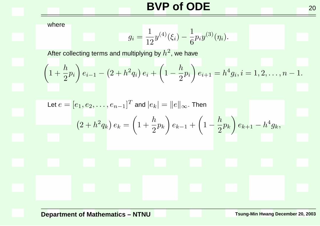
where
gi =1
12y(4)(ξi) −
1
6piy
(3)(ηi).
After collecting terms and multiplying by h2, we have(
1 +h
2pi
)
ei−1 −(
2 + h2qi
)
ei +
(
1 −h
2pi
)
ei+1 = h4gi, i = 1, 2, . . . , n − 1.
Let e = [e1, e2, . . . , en−1]T and |ek| = ‖e‖∞. Then
(
2 + h2qk
)
ek =
(
1 +h
2pk
)
ek−1 +
(
1 −h
2pk
)
ek+1 − h4gk,
and, hence
∣
∣2 + h2qk
∣
∣ |ek| ≤
∣
∣
∣
∣
1 +h
2pk
∣
∣
∣
∣
|ek−1| +
∣
∣
∣
∣
1 −h
2pk
∣
∣
∣
∣
|ek+1| + h4|gk|
≤
∣
∣
∣
∣
1 +h
2pk
∣
∣
∣
∣
‖e‖∞ +
∣
∣
∣
∣
1 −h
2pk
∣
∣
∣
∣
‖e‖∞ + h4‖g‖∞
Department of Mathematics – NTNU Tsung-Min Hwang December 20, 2003

BVP of ODE 20
where
gi =1
12y(4)(ξi) −
1
6piy
(3)(ηi).
After collecting terms and multiplying by h2, we have(
1 +h
2pi
)
ei−1 −(
2 + h2qi
)
ei +
(
1 −h
2pi
)
ei+1 = h4gi, i = 1, 2, . . . , n − 1.
Let e = [e1, e2, . . . , en−1]T and |ek| = ‖e‖∞.
Then
(
2 + h2qk
)
ek =
(
1 +h
2pk
)
ek−1 +
(
1 −h
2pk
)
ek+1 − h4gk,
and, hence
∣
∣2 + h2qk
∣
∣ |ek| ≤
∣
∣
∣
∣
1 +h
2pk
∣
∣
∣
∣
|ek−1| +
∣
∣
∣
∣
1 −h
2pk
∣
∣
∣
∣
|ek+1| + h4|gk|
≤
∣
∣
∣
∣
1 +h
2pk
∣
∣
∣
∣
‖e‖∞ +
∣
∣
∣
∣
1 −h
2pk
∣
∣
∣
∣
‖e‖∞ + h4‖g‖∞
Department of Mathematics – NTNU Tsung-Min Hwang December 20, 2003
BVP of ODE 20
where
gi =1
12y(4)(ξi) −
1
6piy
(3)(ηi).
After collecting terms and multiplying by h2, we have(
1 +h
2pi
)
ei−1 −(
2 + h2qi
)
ei +
(
1 −h
2pi
)
ei+1 = h4gi, i = 1, 2, . . . , n − 1.
Let e = [e1, e2, . . . , en−1]T and |ek| = ‖e‖∞. Then
(
2 + h2qk
)
ek =
(
1 +h
2pk
)
ek−1 +
(
1 −h
2pk
)
ek+1 − h4gk,
and, hence
∣
∣2 + h2qk
∣
∣ |ek| ≤
∣
∣
∣
∣
1 +h
2pk
∣
∣
∣
∣
|ek−1| +
∣
∣
∣
∣
1 −h
2pk
∣
∣
∣
∣
|ek+1| + h4|gk|
≤
∣
∣
∣
∣
1 +h
2pk
∣
∣
∣
∣
‖e‖∞ +
∣
∣
∣
∣
1 −h
2pk
∣
∣
∣
∣
‖e‖∞ + h4‖g‖∞
Department of Mathematics – NTNU Tsung-Min Hwang December 20, 2003

BVP of ODE 20
where
gi =1
12y(4)(ξi) −
1
6piy
(3)(ηi).
After collecting terms and multiplying by h2, we have(
1 +h
2pi
)
ei−1 −(
2 + h2qi
)
ei +
(
1 −h
2pi
)
ei+1 = h4gi, i = 1, 2, . . . , n − 1.
Let e = [e1, e2, . . . , en−1]T and |ek| = ‖e‖∞. Then
(
2 + h2qk
)
ek =
(
1 +h
2pk
)
ek−1 +
(
1 −h
2pk
)
ek+1 − h4gk,
and, hence
∣
∣2 + h2qk
∣
∣ |ek| ≤
∣
∣
∣
∣
1 +h
2pk
∣
∣
∣
∣
|ek−1| +
∣
∣
∣
∣
1 −h
2pk
∣
∣
∣
∣
|ek+1| + h4|gk|
≤
∣
∣
∣
∣
1 +h
2pk
∣
∣
∣
∣
‖e‖∞ +
∣
∣
∣
∣
1 −h
2pk
∣
∣
∣
∣
‖e‖∞ + h4‖g‖∞
Department of Mathematics – NTNU Tsung-Min Hwang December 20, 2003

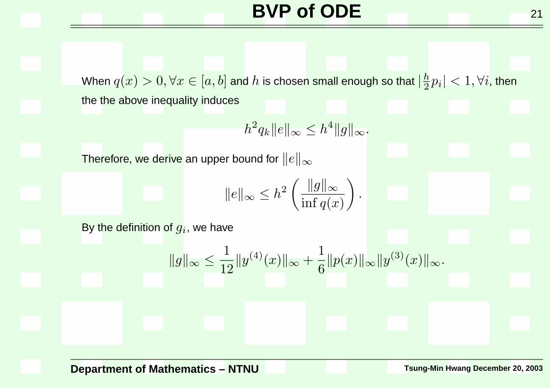
BVP of ODE 21
When q(x) > 0, ∀x ∈ [a, b] and h is chosen small enough so that |h2 pi| < 1, ∀i, then
the the above inequality induces
h2qk‖e‖∞ ≤ h4‖g‖∞.
Therefore, we derive an upper bound for ‖e‖∞
‖e‖∞ ≤ h2
(
‖g‖∞inf q(x)
)
.
By the definition of gi, we have
‖g‖∞ ≤1
12‖y(4)(x)‖∞ +
1
6‖p(x)‖∞‖y(3)(x)‖∞.
Hence‖g‖∞
inf q(x) is a bound independent of h. Thus we can conclude that ‖e‖∞ is O(h2) as
h → 0.
Department of Mathematics – NTNU Tsung-Min Hwang December 20, 2003

BVP of ODE 21
When q(x) > 0, ∀x ∈ [a, b] and h is chosen small enough so that |h2 pi| < 1, ∀i, then
the the above inequality induces
h2qk‖e‖∞ ≤ h4‖g‖∞.
Therefore, we derive an upper bound for ‖e‖∞
‖e‖∞ ≤ h2
(
‖g‖∞inf q(x)
)
.
By the definition of gi, we have
‖g‖∞ ≤1
12‖y(4)(x)‖∞ +
1
6‖p(x)‖∞‖y(3)(x)‖∞.
Hence‖g‖∞
inf q(x) is a bound independent of h.
Thus we can conclude that ‖e‖∞ is O(h2) as
h → 0.
Department of Mathematics – NTNU Tsung-Min Hwang December 20, 2003

BVP of ODE 21
When q(x) > 0, ∀x ∈ [a, b] and h is chosen small enough so that |h2 pi| < 1, ∀i, then
the the above inequality induces
h2qk‖e‖∞ ≤ h4‖g‖∞.
Therefore, we derive an upper bound for ‖e‖∞
‖e‖∞ ≤ h2
(
‖g‖∞inf q(x)
)
.
By the definition of gi, we have
‖g‖∞ ≤1
12‖y(4)(x)‖∞ +
1
6‖p(x)‖∞‖y(3)(x)‖∞.
Hence‖g‖∞
inf q(x) is a bound independent of h. Thus we can conclude that ‖e‖∞ is O(h2) as
h → 0.
Department of Mathematics – NTNU Tsung-Min Hwang December 20, 2003

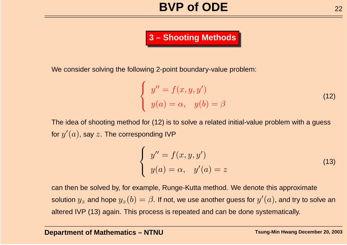
BVP of ODE 22
3 – Shooting Methods
We consider solving the following 2-point boundary-value problem:
y′′ = f(x, y, y′)
y(a) = α, y(b) = β(12)
The idea of shooting method for (12) is to solve a related initial-value problem with a guess
for y′(a), say z. The corresponding IVP
y′′ = f(x, y, y′)
y(a) = α, y′(a) = z(13)
can then be solved by, for example, Runge-Kutta method. We denote this approximate
solution yz and hope yz(b) = β. If not, we use another guess for y′(a), and try to solve an
altered IVP (13) again. This process is repeated and can be done systematically.
Department of Mathematics – NTNU Tsung-Min Hwang December 20, 2003

BVP of ODE 22
3 – Shooting Methods
We consider solving the following 2-point boundary-value problem:
y′′ = f(x, y, y′)
y(a) = α, y(b) = β(12)
The idea of shooting method for (12) is to solve a related initial-value problem with a guess
for y′(a), say z.
The corresponding IVP
y′′ = f(x, y, y′)
y(a) = α, y′(a) = z(13)
can then be solved by, for example, Runge-Kutta method. We denote this approximate
solution yz and hope yz(b) = β. If not, we use another guess for y′(a), and try to solve an
altered IVP (13) again. This process is repeated and can be done systematically.
Department of Mathematics – NTNU Tsung-Min Hwang December 20, 2003

BVP of ODE 22
3 – Shooting Methods
We consider solving the following 2-point boundary-value problem:
y′′ = f(x, y, y′)
y(a) = α, y(b) = β(12)
The idea of shooting method for (12) is to solve a related initial-value problem with a guess
for y′(a), say z. The corresponding IVP
y′′ = f(x, y, y′)
y(a) = α, y′(a) = z(13)
can then be solved by, for example, Runge-Kutta method.
We denote this approximate
solution yz and hope yz(b) = β. If not, we use another guess for y′(a), and try to solve an
altered IVP (13) again. This process is repeated and can be done systematically.
Department of Mathematics – NTNU Tsung-Min Hwang December 20, 2003

BVP of ODE 22
3 – Shooting Methods
We consider solving the following 2-point boundary-value problem:
y′′ = f(x, y, y′)
y(a) = α, y(b) = β(12)
The idea of shooting method for (12) is to solve a related initial-value problem with a guess
for y′(a), say z. The corresponding IVP
y′′ = f(x, y, y′)
y(a) = α, y′(a) = z(13)
can then be solved by, for example, Runge-Kutta method. We denote this approximate
solution yz and hope yz(b) = β.
If not, we use another guess for y′(a), and try to solve an
altered IVP (13) again. This process is repeated and can be done systematically.
Department of Mathematics – NTNU Tsung-Min Hwang December 20, 2003

BVP of ODE 22
3 – Shooting Methods
We consider solving the following 2-point boundary-value problem:
y′′ = f(x, y, y′)
y(a) = α, y(b) = β(12)
The idea of shooting method for (12) is to solve a related initial-value problem with a guess
for y′(a), say z. The corresponding IVP
y′′ = f(x, y, y′)
y(a) = α, y′(a) = z(13)
can then be solved by, for example, Runge-Kutta method. We denote this approximate
solution yz and hope yz(b) = β. If not, we use another guess for y′(a), and try to solve an
altered IVP (13) again.
This process is repeated and can be done systematically.
Department of Mathematics – NTNU Tsung-Min Hwang December 20, 2003
BVP of ODE 22
3 – Shooting Methods
We consider solving the following 2-point boundary-value problem:
y′′ = f(x, y, y′)
y(a) = α, y(b) = β(12)
The idea of shooting method for (12) is to solve a related initial-value problem with a guess
for y′(a), say z. The corresponding IVP
y′′ = f(x, y, y′)
y(a) = α, y′(a) = z(13)
can then be solved by, for example, Runge-Kutta method. We denote this approximate
solution yz and hope yz(b) = β. If not, we use another guess for y′(a), and try to solve an
altered IVP (13) again. This process is repeated and can be done systematically.
Department of Mathematics – NTNU Tsung-Min Hwang December 20, 2003

BVP of ODE 23
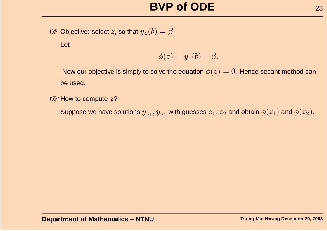
☞ Objective: select z, so that yz(b) = β.
Let
φ(z) = yz(b) − β.
Now our objective is simply to solve the equation φ(z) = 0. Hence secant method can
be used.
☞ How to compute z?
Suppose we have solutions yz1, yz2
with guesses z1, z2 and obtain φ(z1) and φ(z2).
If these guesses can not generate satisfactory solutions, we can obtain another guess
z3 by the secant method
z3 = z2 − φ(z2)z2 − z1
φ(z2) − φ(z1).
In general
zk+1 = zk − φ(zk)zk − zk−1
φ(zk) − φ(zk−1).
Department of Mathematics – NTNU Tsung-Min Hwang December 20, 2003

BVP of ODE 23
☞ Objective: select z, so that yz(b) = β.
Let
φ(z) = yz(b) − β.
Now our objective is simply to solve the equation φ(z) = 0.
Hence secant method can
be used.
☞ How to compute z?
Suppose we have solutions yz1, yz2
with guesses z1, z2 and obtain φ(z1) and φ(z2).
If these guesses can not generate satisfactory solutions, we can obtain another guess
z3 by the secant method
z3 = z2 − φ(z2)z2 − z1
φ(z2) − φ(z1).
In general
zk+1 = zk − φ(zk)zk − zk−1
φ(zk) − φ(zk−1).
Department of Mathematics – NTNU Tsung-Min Hwang December 20, 2003

BVP of ODE 23
☞ Objective: select z, so that yz(b) = β.
Let
φ(z) = yz(b) − β.
Now our objective is simply to solve the equation φ(z) = 0. Hence secant method can
be used.
☞ How to compute z?
Suppose we have solutions yz1, yz2
with guesses z1, z2 and obtain φ(z1) and φ(z2).
If these guesses can not generate satisfactory solutions, we can obtain another guess
z3 by the secant method
z3 = z2 − φ(z2)z2 − z1
φ(z2) − φ(z1).
In general
zk+1 = zk − φ(zk)zk − zk−1
φ(zk) − φ(zk−1).
Department of Mathematics – NTNU Tsung-Min Hwang December 20, 2003

BVP of ODE 23
☞ Objective: select z, so that yz(b) = β.
Let
φ(z) = yz(b) − β.
Now our objective is simply to solve the equation φ(z) = 0. Hence secant method can
be used.
☞ How to compute z?
Suppose we have solutions yz1, yz2
with guesses z1, z2 and obtain φ(z1) and φ(z2).
If these guesses can not generate satisfactory solutions, we can obtain another guess
z3 by the secant method
z3 = z2 − φ(z2)z2 − z1
φ(z2) − φ(z1).
In general
zk+1 = zk − φ(zk)zk − zk−1
φ(zk) − φ(zk−1).
Department of Mathematics – NTNU Tsung-Min Hwang December 20, 2003

BVP of ODE 24
☞ Special BVP:
y′′ = u(x) + v(x)y + w(x)y′
y(a) = α, y(b) = β(14)
where u(x), v(x), w(x) are continuous in [a, b].
Suppose we have solved (14) twice with initial guesses z1 and z2, and obtain
approximate solutions y1 and y2, hence
y1′′ = u + vy1 + wy1
′
y1(a) = α, y1′(a) = z1
and
y2′′ = u + vy2 + wy2
′
y2(a) = α, y2′(a) = z2
Now let
y(x) = λy1(x) + (1 − λ)y2(x)
for some parameter λ, we can show
y′′ = u + vy + wy′
Department of Mathematics – NTNU Tsung-Min Hwang December 20, 2003

BVP of ODE 24
☞ Special BVP:
y′′ = u(x) + v(x)y + w(x)y′
y(a) = α, y(b) = β(14)
where u(x), v(x), w(x) are continuous in [a, b].
Suppose we have solved (14) twice with initial guesses z1 and z2, and obtain
approximate solutions y1 and y2,
hence
y1′′ = u + vy1 + wy1
′
y1(a) = α, y1′(a) = z1
and
y2′′ = u + vy2 + wy2
′
y2(a) = α, y2′(a) = z2
Now let
y(x) = λy1(x) + (1 − λ)y2(x)
for some parameter λ, we can show
y′′ = u + vy + wy′
Department of Mathematics – NTNU Tsung-Min Hwang December 20, 2003

BVP of ODE 24
☞ Special BVP:
y′′ = u(x) + v(x)y + w(x)y′
y(a) = α, y(b) = β(14)
where u(x), v(x), w(x) are continuous in [a, b].
Suppose we have solved (14) twice with initial guesses z1 and z2, and obtain
approximate solutions y1 and y2, hence
y1′′ = u + vy1 + wy1
′
y1(a) = α, y1′(a) = z1
and
y2′′ = u + vy2 + wy2
′
y2(a) = α, y2′(a) = z2
Now let
y(x) = λy1(x) + (1 − λ)y2(x)
for some parameter λ, we can show
y′′ = u + vy + wy′
Department of Mathematics – NTNU Tsung-Min Hwang December 20, 2003

BVP of ODE 24
☞ Special BVP:
y′′ = u(x) + v(x)y + w(x)y′
y(a) = α, y(b) = β(14)
where u(x), v(x), w(x) are continuous in [a, b].
Suppose we have solved (14) twice with initial guesses z1 and z2, and obtain
approximate solutions y1 and y2, hence
y1′′ = u + vy1 + wy1
′
y1(a) = α, y1′(a) = z1
and
y2′′ = u + vy2 + wy2
′
y2(a) = α, y2′(a) = z2
Now let
y(x) = λy1(x) + (1 − λ)y2(x)
for some parameter λ,
we can show
y′′ = u + vy + wy′
Department of Mathematics – NTNU Tsung-Min Hwang December 20, 2003

BVP of ODE 24
☞ Special BVP:
y′′ = u(x) + v(x)y + w(x)y′
y(a) = α, y(b) = β(14)
where u(x), v(x), w(x) are continuous in [a, b].
Suppose we have solved (14) twice with initial guesses z1 and z2, and obtain
approximate solutions y1 and y2, hence
y1′′ = u + vy1 + wy1
′
y1(a) = α, y1′(a) = z1
and
y2′′ = u + vy2 + wy2
′
y2(a) = α, y2′(a) = z2
Now let
y(x) = λy1(x) + (1 − λ)y2(x)
for some parameter λ, we can show
y′′ = u + vy + wy′
Department of Mathematics – NTNU Tsung-Min Hwang December 20, 2003

BVP of ODE 25
and
y(a) = λy1(a) + (1 − λ)y2(a) = α
We can select λ so that y(b) = β.
β = y(b) = λy1(b) + (1 − λ)y2(b)
= λ(y1(b) − y2(b)) + y2(b)
⇒ λ =β − y2(b)
(y1(b) − y2(b))
In practice, we can solve the following two IVPs (in parallel)
y′′ = u(x) + v(x)y + w(x)y′
y(a) = α, y′(a) = 0
and
y′′ = u(x) + v(x)y + w(x)y′
y(a) = α, y′(a) = 1
Department of Mathematics – NTNU Tsung-Min Hwang December 20, 2003

BVP of ODE 26
i.e.,
y′1 = y3
y3′ = y1
′′ = u + vy1 + wy1′ = u + vy1 + wy3
y1(a) = α, y3(a) = y1′(a) = 0
and
y2′ = y4
y4′ = u + vy2 + wy4
y2(a) = α, y4(a) = 1
to obtain approximate solutions y1 and y2, then compute λ and form the solution y.
Department of Mathematics – NTNU Tsung-Min Hwang December 20, 2003