简介 I Introduction - CUHKkthau/download/483 SEM AMOS total Oct 2009 handout... · Amos KT Hau Chinese University of Hong Kong 2010/9/3 3 KT HAU SEM p. 13 Additional notes on EFA

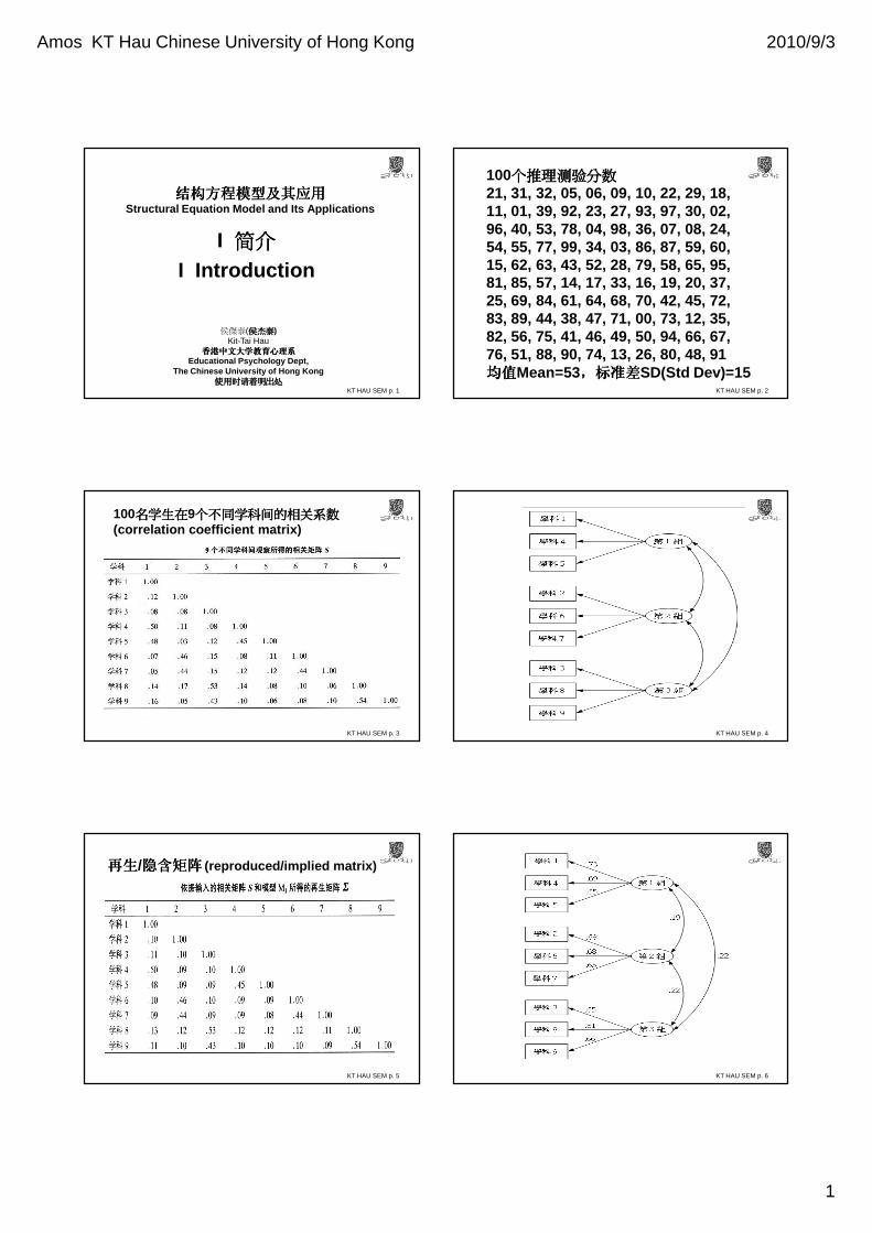
Amos KT Hau Chinese University of Hong Kong 2010/9/3

1

KT HAU SEM p. 1

结构方程模型及其应用结构方程模型及其应用结构方程模型及其应用结构方程模型及其应用Structural Equation Model and Its Applications

I 简介简介简介简介

I Introduction

侯傑泰(侯杰泰侯杰泰侯杰泰侯杰泰)Kit-Tai Hau

香港中文大学教育心理系香港中文大学教育心理系香港中文大学教育心理系香港中文大学教育心理系Educational Psychology Dept,

The Chinese University of Hong Kong使用时请着明出处使用时请着明出处使用时请着明出处使用时请着明出处

KT HAU SEM p. 2

100个推理测验分数个推理测验分数个推理测验分数个推理测验分数21, 31, 32, 05, 06, 09, 10, 22, 29, 18, 11, 01, 39, 92, 23, 27, 93, 97, 30, 02,96, 40, 53, 78, 04, 98, 36, 07, 08, 24,54, 55, 77, 99, 34, 03, 86, 87, 59, 60,15, 62, 63, 43, 52, 28, 79, 58, 65, 95, 81, 85, 57, 14, 17, 33, 16, 19, 20, 37, 25, 69, 84, 61, 64, 68, 70, 42, 45, 72,83, 89, 44, 38, 47, 71, 00, 73, 12, 35,82, 56, 75, 41, 46, 49, 50, 94, 66, 67, 76, 51, 88, 90, 74, 13, 26, 80, 48, 91 均值均值均值均值Mean=53，，，，标准差标准差标准差标准差SD(Std Dev)=15

KT HAU SEM p. 3

100名学生在名学生在名学生在名学生在9个不同学科间的相关系数个不同学科间的相关系数个不同学科间的相关系数个不同学科间的相关系数(correlation coefficient matrix)

KT HAU SEM p. 4

KT HAU SEM p. 5

再生再生再生再生/隐含矩阵隐含矩阵隐含矩阵隐含矩阵 (reproduced/implied matrix)

KT HAU SEM p. 6


2

KT HAU SEM p. 7 KT HAU SEM p. 8

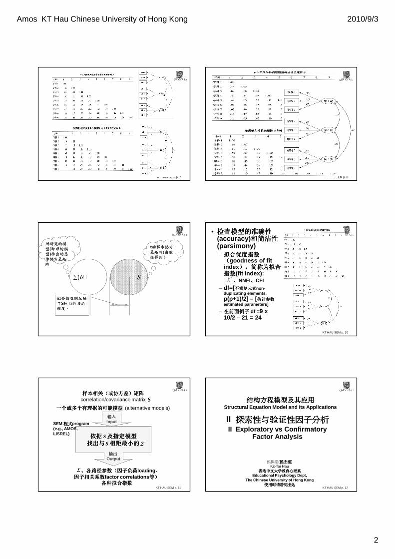
拟合指数则反映拟合指数则反映了了SS和和接近接近程度。程度。

xx的样本协方的样本协方差矩阵差矩阵((由数由数据得到）据得到）

SS

( )θ∑

所研究的模所研究的模型型((即理论模即理论模型型))推出的总推出的总体协方差矩体协方差矩阵阵

∑(θ)

KT HAU SEM p. 10

• 检查模型的准确性检查模型的准确性检查模型的准确性检查模型的准确性(accuracy) 和简洁性和简洁性和简洁性和简洁性(parsimony)– 拟合优度指数拟合优度指数拟合优度指数拟合优度指数（（（（goodness of fit index ），），），），简称为拟合简称为拟合简称为拟合简称为拟合指数指数指数指数(fit index):

、、、、NNFI、、、、CFI– df=[ 不重复元素不重复元素不重复元素不重复元素non-

duplicating elements,p(p+1)/2] – [ 估计参数估计参数估计参数估计参数estimated parameters]

– 在前面例子在前面例子在前面例子在前面例子 df =9 x 10/2 – 21 = 24

2χ

KT HAU SEM p. 11

依据依据依据依据及指定模型及指定模型及指定模型及指定模型找出与找出与找出与找出与相距最小的相距最小的相距最小的相距最小的

样本相关样本相关样本相关样本相关（（（（或协方差或协方差或协方差或协方差））））矩阵矩阵矩阵矩阵correlation/covariance matrix

一个或多个有理据的可能模型一个或多个有理据的可能模型一个或多个有理据的可能模型一个或多个有理据的可能模型 (alternative models)

ΣSS

输出输出输出输出Output

输入输入输入输入InputSEM 程式程式程式程式program

(e.g., AMOS, LISREL)

S

、、、、各路径参数各路径参数各路径参数各路径参数（（（（因子负荷因子负荷因子负荷因子负荷loading 、、、、

因子相关系数因子相关系数因子相关系数因子相关系数factor correlations 等等等等））））各种拟合指数各种拟合指数各种拟合指数各种拟合指数

Σ

KT HAU SEM p. 12


II 探索性与验证性因探索性与验证性因探索性与验证性因探索性与验证性因子子子子分析分析分析分析II Exploratory vs Confirmatory

Factor Analysis





3

KT HAU SEM p. 13

Additional notes on EFA

Exploratory Factor Analyses (EFA)• In the above analyses, we have a

structure in mind to test, this process is called confirmatory factor analysis (CFA)

• It is also possible that we have no “theory”in mind to test, i.e., we have the following research questions:– How many cluster of subjects are there? How

do these 9 subjects relate to each of these clusters (factors)?

– Which of these subjects are more closely related/correlated than others?

KT HAU SEM p. 14

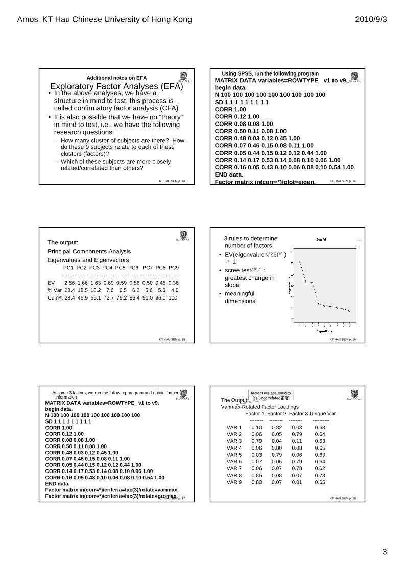
Using SPSS, run the following program MATRIX DATA variables=ROWTYPE_ v1 to v9.begin data.N 100 100 100 100 100 100 100 100 100SD 1 1 1 1 1 1 1 1 1CORR 1.00CORR 0.12 1.00CORR 0.08 0.08 1.00CORR 0.50 0.11 0.08 1.00CORR 0.48 0.03 0.12 0.45 1.00CORR 0.07 0.46 0.15 0.08 0.11 1.00CORR 0.05 0.44 0.15 0.12 0.12 0.44 1.00CORR 0.14 0.17 0.53 0.14 0.08 0.10 0.06 1.00CORR 0.16 0.05 0.43 0.10 0.06 0.08 0.10 0.54 1.00END data.Factor matrix in(corr=*)/plot=eigen.

KT HAU SEM p. 15

The output:

Principal Components Analysis

Eigenvalues and EigenvectorsPC1 PC2 PC3 PC4 PC5 PC6 PC7 PC8 PC9 ------ ------ ------ ------ ------ ------ ------ ------ ------

EV 2.56 1.66 1.63 0.69 0.59 0.56 0.50 0.45 0.36% Var 28.4 18.5 18.2 7.6 6.5 6.2 5.6 5.0 4.0Cum% 28.4 46.9 65.1 72.7 79.2 85.4 91.0 96.0 100.

KT HAU SEM p. 16

3 rules to determine number of factors

• EV(eigenvalue特征值 ) ≧ 1

• scree test碎石: greatest change inslope

• meaningful dimensions

KT HAU SEM p. 17

Assume 3 factors, we run the following program and obtain further information

MATRIX DATA variables=ROWTYPE_ v1 to v9.begin data.N 100 100 100 100 100 100 100 100 100SD 1 1 1 1 1 1 1 1 1CORR 1.00CORR 0.12 1.00CORR 0.08 0.08 1.00CORR 0.50 0.11 0.08 1.00CORR 0.48 0.03 0.12 0.45 1.00CORR 0.07 0.46 0.15 0.08 0.11 1.00CORR 0.05 0.44 0.15 0.12 0.12 0.44 1.00CORR 0.14 0.17 0.53 0.14 0.08 0.10 0.06 1.00CORR 0.16 0.05 0.43 0.10 0.06 0.08 0.10 0.54 1.00END data.Factor matrix in(corr=*)/criteria=fac(3)/rotate=var imax.Factor matrix in(corr=*)/criteria=fac(3)/rotate=pro max. KT HAU SEM p. 18

The Output:Varimax-Rotated Factor Loadings

Factor 1 Factor 2 Factor 3 Unique Var-------- -------- -------- ----------

VAR 1 0.10 0.82 0.03 0.68VAR 2 0.06 0.05 0.79 0.64VAR 3 0.79 0.04 0.11 0.63VAR 4 0.06 0.80 0.08 0.65VAR 5 0.03 0.79 0.06 0.63VAR 6 0.07 0.05 0.79 0.64VAR 7 0.06 0.07 0.78 0.62VAR 8 0.85 0.08 0.07 0.73VAR 9 0.80 0.07 0.01 0.65

factors are assumed to be uncorrelated正交正交正交正交


4

KT HAU SEM p. 19

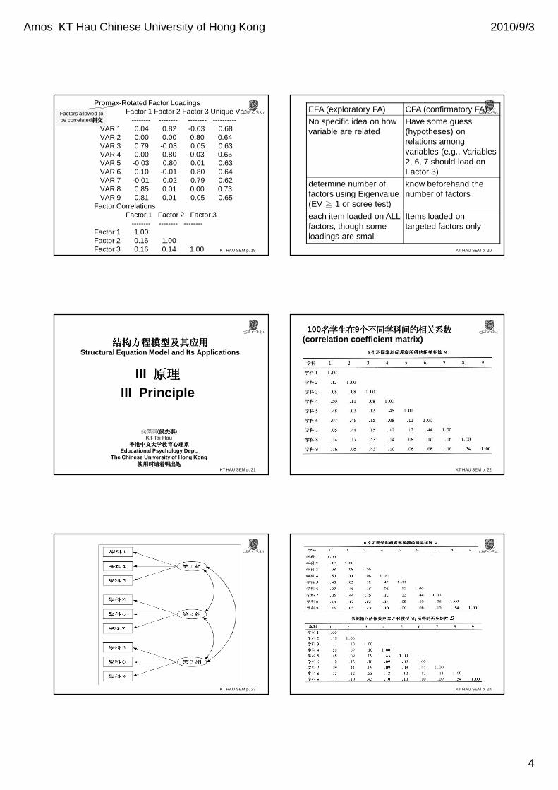
Promax-Rotated Factor LoadingsFactor 1 Factor 2 Factor 3 Unique Var

-------- -------- -------- ----------VAR 1 0.04 0.82 -0.03 0.68VAR 2 0.00 0.00 0.80 0.64VAR 3 0.79 -0.03 0.05 0.63VAR 4 0.00 0.80 0.03 0.65VAR 5 -0.03 0.80 0.01 0.63VAR 6 0.10 -0.01 0.80 0.64VAR 7 -0.01 0.02 0.79 0.62VAR 8 0.85 0.01 0.00 0.73VAR 9 0.81 0.01 -0.05 0.65

Factor Correlations Factor 1 Factor 2 Factor 3

-------- -------- --------Factor 1 1.00Factor 2 0.16 1.00Factor 3 0.16 0.14 1.00

Factors allowed to be correlated斜交斜交斜交斜交

KT HAU SEM p. 20

EFA (exploratory FA) CFA (confirmatory FA)

No specific idea on how variable are related

Have some guess (hypotheses) on relations among variables (e.g., Variables 2, 6, 7 should load on Factor 3)

determine number of factors using Eigenvalue (EV ≧ 1 or scree test)

know beforehand the number of factors

each item loaded on ALL factors, though some loadings are small

Items loaded on targeted factors only

KT HAU SEM p. 21


III 原原原原理理理理

III Principle




KT HAU SEM p. 22

100名学生在名学生在名学生在名学生在9个不同学科间的相关系数个不同学科间的相关系数个不同学科间的相关系数个不同学科间的相关系数(correlation coefficient matrix)



5





6



_________________________________________________________________________________________________

(no. of estimated parameters)模型模型模型模型 df NNFI CFI 需要估计的参数个数需要估计的参数个数需要估计的参数个数需要估计的参数个数

2χ______________________________________________________________________________________________

M1 24 40 .973 .982 21 = 9 Load + 9 Uniq + 3 Corr

M2 27 503 .294 .471 18 = 9 Load + 9 Uniq

M3 26 255 .647 .745 19 = 9 Load + 9 Uniq + 1 Corr

M4 26 249 .656 .752 19 = 9 Load + 9 Uniq + 1 Corr

M5 27 263 .649 .727 18 = 9 Load + 9 Uniq

M6 24 422 .337 .558 21 = 9 Load + 9 Uniq + 3 Corr

M7 21 113 .826 .898 24 = 9 Load + 9 Uniq + 6 Corr______________________________________________________________________________________________

KT HAU SEM p. 35

模型比较 (Model Comparison)• 自由度(df), 拟合程度 (fit), 不能保证最好，可能存在更简洁(parsimonious) 又拟合(fit)得很好的模型

• 输入输入输入输入Input:– 相关（或协方差）矩阵correlation/covariance

matrix

– 一个或多个有理据的可能模型 (alternative models)

• 输出输出输出输出Output:– 既符合某指定模型，又与差异最小的矩阵

– 估计各路径参数parameter（因子负荷loading、因子相关系数factor correlations等）。

– 计算出各种拟合指数(goodness of fit indexes)

Σ

S

S

KT HAU SEM p. 36

依据依据依据依据及指定模型及指定模型及指定模型及指定模型找出与找出与找出与找出与相距最小的相距最小的相距最小的相距最小的

样本相关样本相关样本相关样本相关（（（（或协方差或协方差或协方差或协方差））））矩阵矩阵矩阵矩阵correlation/covariance matrix

一个或多个有理据的可能模型一个或多个有理据的可能模型一个或多个有理据的可能模型一个或多个有理据的可能模型 (alternative models)

ΣSS

输出输出输出输出Output

输入输入输入输入InputSEM 程式程式程式程式program

(e.g., LISREL)

S

、、、、各路径参数各路径参数各路径参数各路径参数（（（（因子负荷因子负荷因子负荷因子负荷loading 、、、、

因子相关系数因子相关系数因子相关系数因子相关系数factor correlations 等等等等））））各种拟合指数各种拟合指数各种拟合指数各种拟合指数

Σ


7

KT HAU SEM p. 37

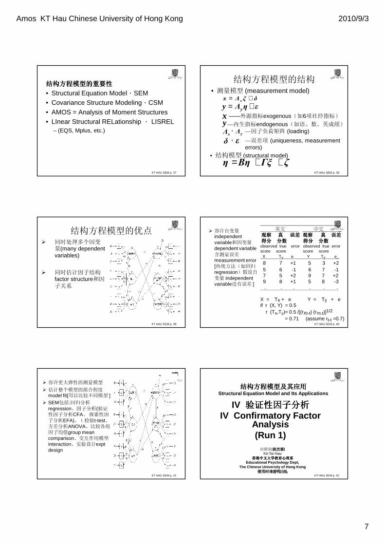
结构方程模型的重要性结构方程模型的重要性结构方程模型的重要性结构方程模型的重要性

• Structural Equation Model，SEM• Covariance Structure Modeling，CSM

• AMOS = Analysis of Moment Structures• LInear Structural RELationship ， LISREL

– (EQS, Mplus, etc.)

KT HAU SEM p. 38

结构方程模型的结构• 测量模型 (measurement model)

,,

δξΛx x +=εηΛy y +=

x ——外源指标exogenous（如6项社经指标）

y —内生指标endogenous（如语、数、英成绩）

xΛ yΛ

δ ε —误差项 (uniqueness, measurement errors)

• 结构模型 (structural model)ζΓξΒηη ++=

KT HAU SEM p. 39

结构方程模型的优点� 同时处理多个因变

量(many dependent variables)

� 同时估计因子结构factor structure和因子关系

KT HAU SEM p. 40

� 容许自变量independent variable和因变量dependent variable含测量误差measurement error [传统方法（如回归regression）假设自变量 independent variable没有误差 ]

_______________________________________

英文中文 _观察观察观察观察真真真真误差误差误差误差观察观察观察观察真真真真误差误差误差误差得分得分得分得分分数分数分数分数得分得分得分得分分数分数分数分数observed true error observed true errorscore score score scoreX Tx e Y Ty e_

8 7 +1 5 3 +25 6 -1 6 7 -17 5 +2 9 7 +29 8 +1 5 8 -3. . . . . .

X = Tx + e Y = Ty + eif r (X, Y) = 0.5

r (Tx,Ty)= 0.5 /[(rXt-t) (rYt-t)]1/2

= 0.71 (assume rt-t =0.7)

KT HAU SEM p. 41

� 容许更大弹性的测量模型

� 估计整个模型的拟合程度model fit[用以比较不同模型 ]

� SEM包括:回归分析regression、因子分析(验证性因子分析CFA、探索性因子分析EFA)、ｔ检验t-test、方差分析ANOVA、比较各组因子均值group mean comparison、交互作用模型interaction、实验设计expt design

KT HAU SEM p. 42


IV 验证性因子分析验证性因子分析验证性因子分析验证性因子分析IV Confirmatory Factor

Analysis(Run 1)





8

KT HAU SEM p. 43

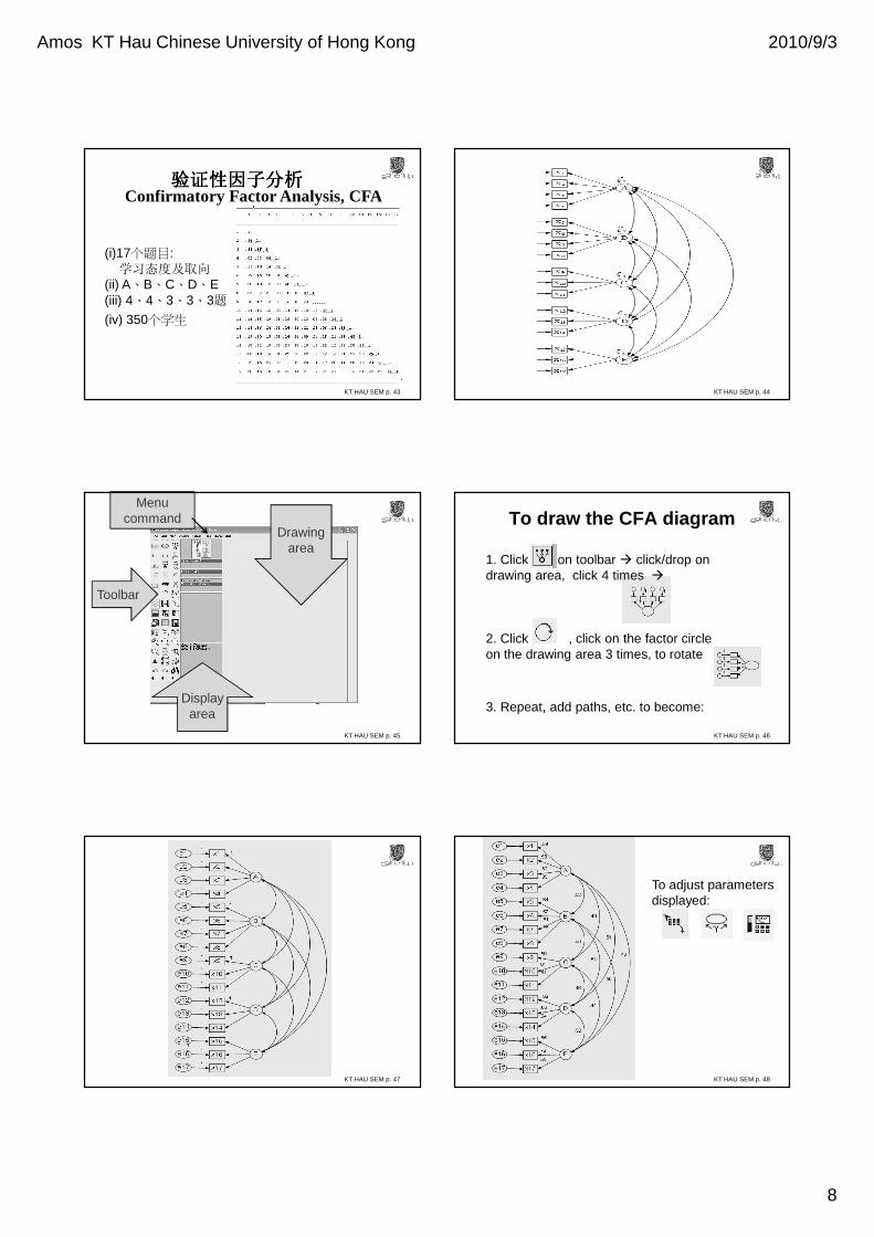
验证性因子分析验证性因子分析验证性因子分析验证性因子分析

(i)17个题目:学习态度及取向

(ii) A、B、C、D、E(iii) 4、4、3、3、3题

(iv) 350个学生

Confirmatory Factor Analysis, CFA

KT HAU SEM p. 44

KT HAU SEM p. 45

Menu command

Toolbar

Drawing area

Display area

To draw the CFA diagram

KT HAU SEM p. 46

1. Click on toolbar � click/drop on drawing area, click 4 times �

2. Click , click on the factor circle on the drawing area 3 times, to rotate

3. Repeat, add paths, etc. to become:


To adjust parameters displayed:


9

KT HAU SEM p. 49

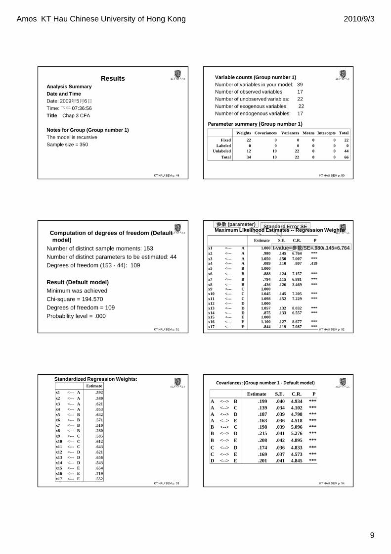
ResultsAnalysis SummaryDate and TimeDate: 2009年5月6日

Time: 下午 07:36:56Title Chap 3 CFA

Notes for Group (Group number 1)The model is recursiveSample size = 350

KT HAU SEM p. 50

Variable counts (Group number 1)Number of variables in your model: 39Number of observed variables: 17Number of unobserved variables: 22Number of exogenous variables: 22Number of endogenous variables: 17

Weights Covariances Variances Means Intercepts Total

Fixed 22 0 0 0 0 22Labeled 0 0 0 0 0 0

Unlabeled 12 10 22 0 0 44

Total 34 10 22 0 0 66

Parameter summary (Group number 1)

Computation of degrees of freedom (Default model)

Number of distinct sample moments: 153

Number of distinct parameters to be estimated: 44

Degrees of freedom (153 - 44): 109

Result (Default model)Minimum was achieved

Chi-square = 194.570

Degrees of freedom = 109

Probability level = .000

KT HAU SEM p. 51

Standard Error SE参数参数参数参数 (parameter)

KT HAU SEM p. 52

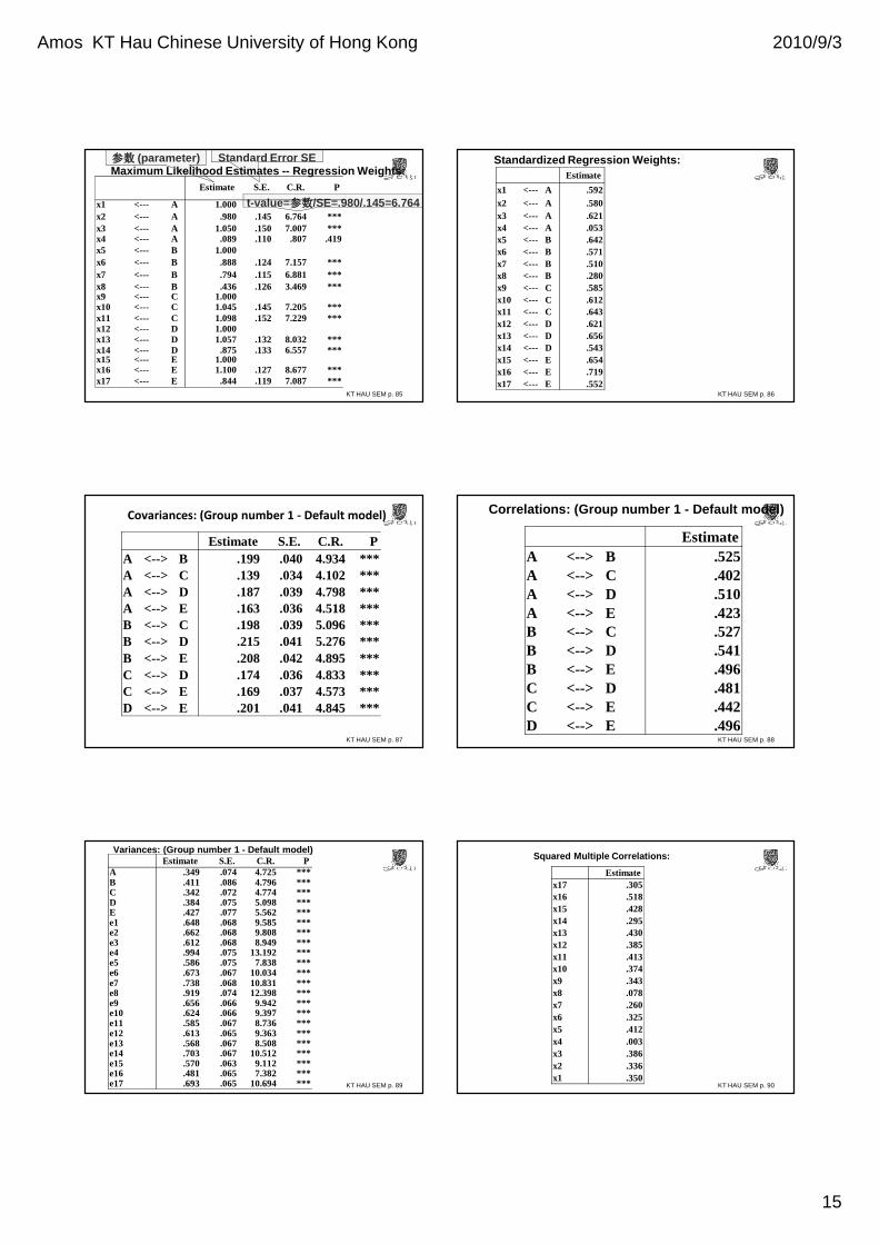
Maximum Likelihood Estimates -- Regression Weights:

t-value=参数参数参数参数/SE=.980/.145=6.764

Estimate S.E. C.R. P

x1 <--- A 1.000x2 <--- A .980 .145 6.764 ***x3 <--- A 1.050 .150 7.007 ***x4 <--- A .089 .110 .807 .419x5 <--- B 1.000x6 <--- B .888 .124 7.157 ***x7 <--- B .794 .115 6.881 ***x8 <--- B .436 .126 3.469 ***x9 <--- C 1.000x10 <--- C 1.045 .145 7.205 ***x11 <--- C 1.098 .152 7.229 ***x12 <--- D 1.000x13 <--- D 1.057 .132 8.032 ***x14 <--- D .875 .133 6.557 ***x15 <--- E 1.000x16 <--- E 1.100 .127 8.677 ***x17 <--- E .844 .119 7.087 ***

Standardized Regression Weights:

KT HAU SEM p. 53

Estimate

x1 <--- A .592x2 <--- A .580x3 <--- A .621x4 <--- A .053x5 <--- B .642x6 <--- B .571x7 <--- B .510x8 <--- B .280x9 <--- C .585x10 <--- C .612x11 <--- C .643x12 <--- D .621x13 <--- D .656x14 <--- D .543x15 <--- E .654x16 <--- E .719x17 <--- E .552

KT HAU SEM p. 54

Covariances: (Group number 1 - Default model)

Estimate S.E. C.R. P

A <--> B .199 .040 4.934 ***A <--> C .139 .034 4.102 ***A <--> D .187 .039 4.798 ***A <--> E .163 .036 4.518 ***B <--> C .198 .039 5.096 ***B <--> D .215 .041 5.276 ***B <--> E .208 .042 4.895 ***

C <--> D .174 .036 4.833 ***C <--> E .169 .037 4.573 ***D <--> E .201 .041 4.845 ***


10

KT HAU SEM p. 55

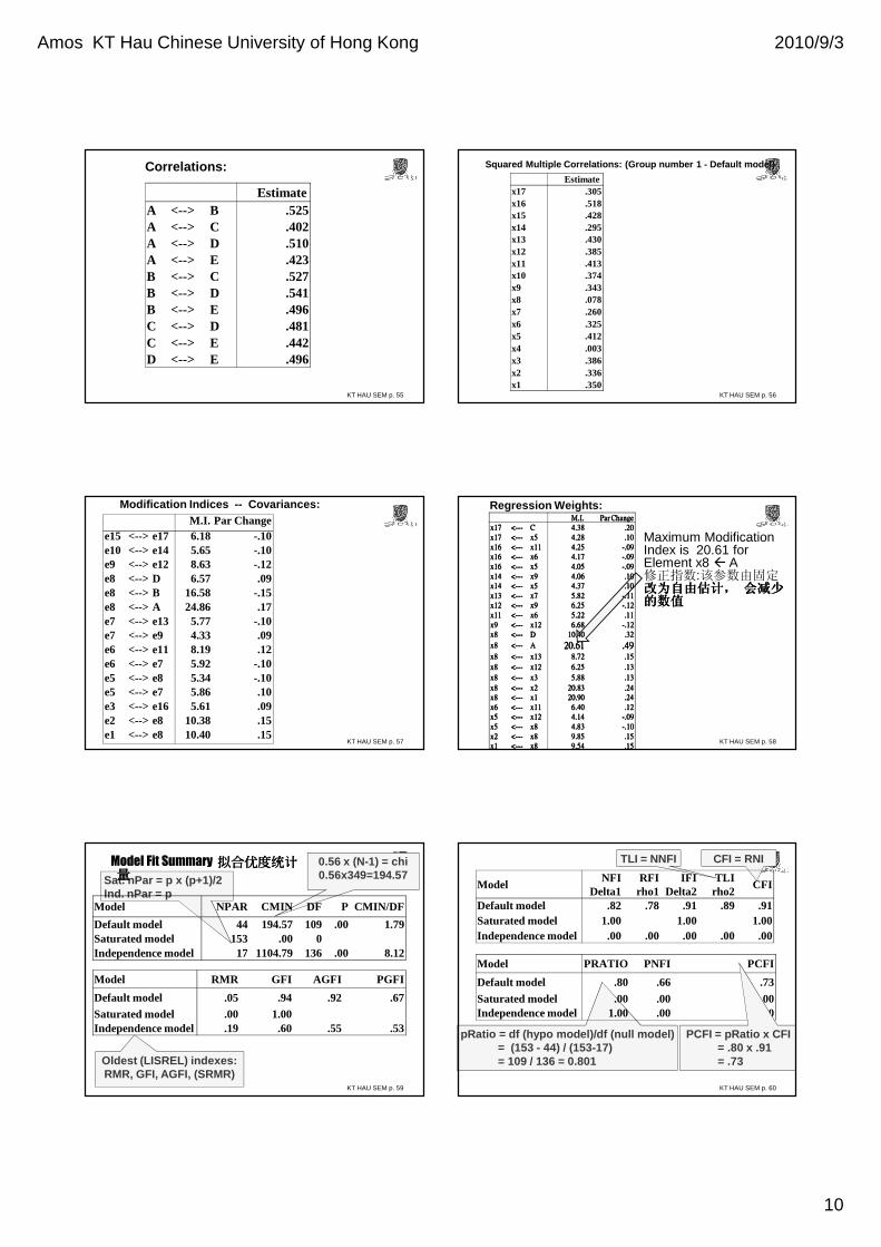
Correlations:

EstimateA <--> B .525A <--> C .402A <--> D .510A <--> E .423B <--> C .527B <--> D .541B <--> E .496C <--> D .481C <--> E .442D <--> E .496

KT HAU SEM p. 56

Squared Multiple Correlations: (Group number 1 - Def ault model)

Estimatex17 .305x16 .518x15 .428x14 .295x13 .430x12 .385x11 .413x10 .374x9 .343x8 .078x7 .260x6 .325x5 .412x4 .003x3 .386x2 .336x1 .350

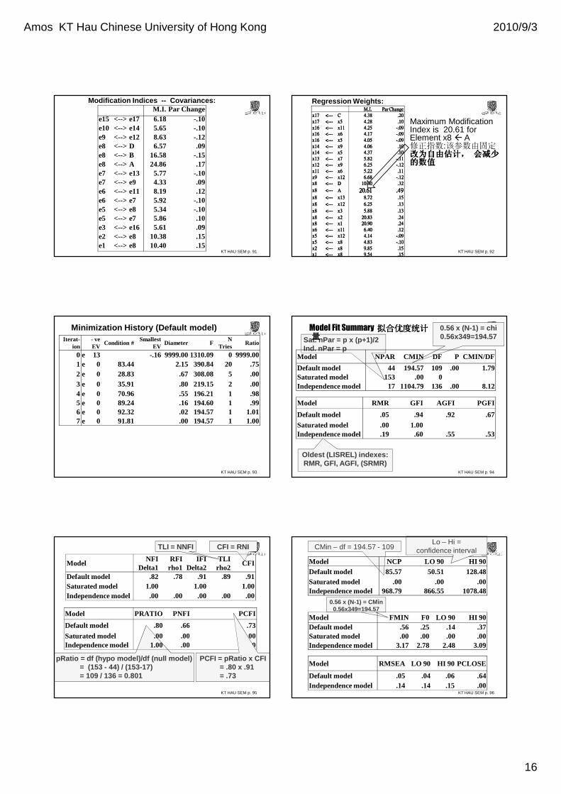
Modification Indices -- Covariances:

KT HAU SEM p. 57

M.I. Par Changee15 <--> e17 6.18 -.10e10 <--> e14 5.65 -.10e9 <--> e12 8.63 -.12e8 <--> D 6.57 .09e8 <--> B 16.58 -.15e8 <--> A 24.86 .17e7 <--> e13 5.77 -.10e7 <--> e9 4.33 .09e6 <--> e11 8.19 .12e6 <--> e7 5.92 -.10e5 <--> e8 5.34 -.10e5 <--> e7 5.86 .10e3 <--> e16 5.61 .09e2 <--> e8 10.38 .15e1 <--> e8 10.40 .15

Regression Weights:M.I.M.I.M.I.M.I. Par ChangePar ChangePar ChangePar Change

x17x17x17x17 <<<<------------ CCCC 4.384.384.384.38 .20.20.20.20

x17x17x17x17 <<<<------------ x5x5x5x5 4.284.284.284.28 .10.10.10.10

x16x16x16x16 <<<<------------ x11x11x11x11 4.254.254.254.25 ----.09.09.09.09

x16x16x16x16 <<<<------------ x6x6x6x6 4.174.174.174.17 ----.09.09.09.09

x16x16x16x16 <<<<------------ x5x5x5x5 4.054.054.054.05 ----.09.09.09.09

x14x14x14x14 <<<<------------ x9x9x9x9 4.064.064.064.06 .10.10.10.10

x14x14x14x14 <<<<------------ x5x5x5x5 4.374.374.374.37 .10.10.10.10

x13x13x13x13 <<<<------------ x7x7x7x7 5.825.825.825.82 ----.11.11.11.11

x12x12x12x12 <<<<------------ x9x9x9x9 6.256.256.256.25 ----.12.12.12.12

x11x11x11x11 <<<<------------ x6x6x6x6 5.225.225.225.22 .11.11.11.11

x9x9x9x9 <<<<------------ x12x12x12x12 6.686.686.686.68 ----.12.12.12.12

x8x8x8x8 <<<<------------ DDDD 10.4010.4010.4010.40 .32.32.32.32

x8x8x8x8 <<<<------------ AAAA 20.6120.6120.6120.61 .49.49.49.49x8x8x8x8 <<<<------------ x13x13x13x13 8.728.728.728.72 .15.15.15.15

x8x8x8x8 <<<<------------ x12x12x12x12 6.256.256.256.25 .13.13.13.13

x8x8x8x8 <<<<------------ x3x3x3x3 5.885.885.885.88 .13.13.13.13

x8x8x8x8 <<<<------------ x2x2x2x2 20.8320.8320.8320.83 .24.24.24.24

x8x8x8x8 <<<<------------ x1x1x1x1 20.9020.9020.9020.90 .24.24.24.24

x6x6x6x6 <<<<------------ x11x11x11x11 6.406.406.406.40 .12.12.12.12

x5x5x5x5 <<<<------------ x12x12x12x12 4.144.144.144.14 ----.09.09.09.09

x5x5x5x5 <<<<------------ x8x8x8x8 4.834.834.834.83 ----.10.10.10.10

x2x2x2x2 <<<<------------ x8x8x8x8 9.859.859.859.85 .15.15.15.15

x1x1x1x1 <<<<------------ x8x8x8x8 9.549.549.549.54 .15.15.15.15KT HAU SEM p. 58

Maximum Modification Index is 20.61 for Element x8 A修正指数:该参数由固定改为自由估计改为自由估计改为自由估计改为自由估计，，，，会减少会减少会减少会减少的数值的数值的数值的数值

Sat. nPar = p x (p+1)/2Ind. nPar = p

0.56 x (N-1) = chi0.56x349=194.57

KT HAU SEM p. 59

Model Fit Summary 拟合优度统计拟合优度统计拟合优度统计拟合优度统计量量量量

Model NPAR CMIN DF P CMIN/DF

Default model 44 194.57 109 .00 1.79Saturated model 153 .00 0Independence model 17 1104.79 136 .00 8.12

Model RMR GFI AGFI PGFI

Default model .05 .94 .92 .67Saturated model .00 1.00Independence model .19 .60 .55 .53

Oldest (LISREL) indexes: RMR, GFI, AGFI, (SRMR)

pRatio = df (hypo model)/df (null model)= (153 - 44) / (153-17)= 109 / 136 = 0.801

KT HAU SEM p. 60

TLI = NNFI CFI = RNI

ModelNFI

Delta1RFI

rho1IFI

Delta2TLI

rho2CFI

Default model .82 .78 .91 .89 .91Saturated model 1.00 1.00 1.00Independence model .00 .00 .00 .00 .00

Model PRATIO PNFI PCFI

Default model .80 .66 .73

Saturated model .00 .00 .00Independence model 1.00 .00 .00

PCFI = pRatio x CFI= .80 x .91= .73


11

KT HAU Amos p. 61

Completely Standardized Solution

KT HAU SEM p. 62

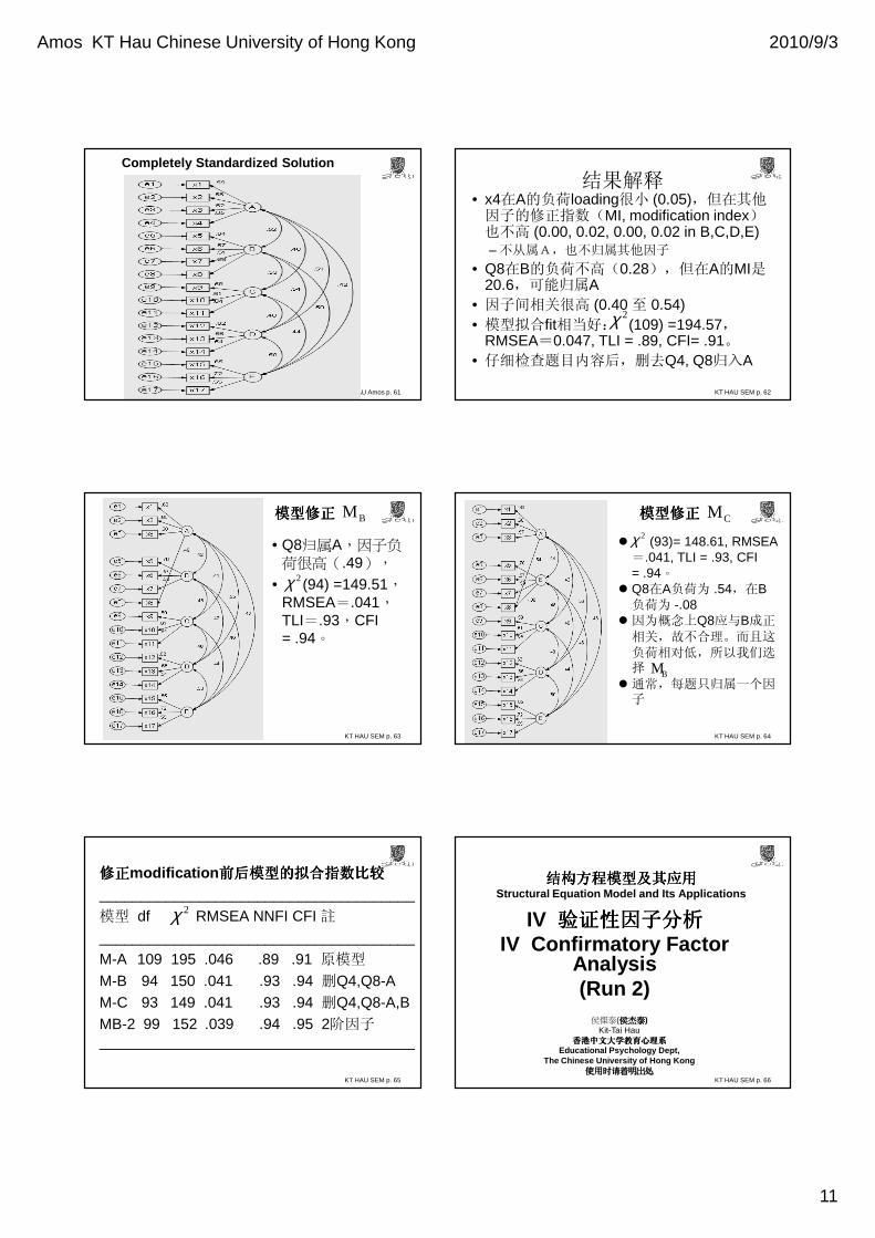
结果解释• x4在A的负荷loading很小 (0.05)，但在其他因子的修正指数（MI, modification index）也不高 (0.00, 0.02, 0.00, 0.02 in B,C,D,E)– 不从属Ａ，也不归属其他因子

• Q8在B的负荷不高（0.28），但在A的MI是20.6，可能归属A

• 因子间相关很高 (0.40 至 0.54)• 模型拟合fit相当好： (109) =194.57，

RMSEA＝0.047, TLI = .89, CFI= .91。• 仔细检查题目内容后，删去Q4, Q8归入A

2χ

KT HAU SEM p. 63

2χ

• Q8归属A，因子负荷很高（.49），

• (94) =149.51，RMSEA＝.041，TLI＝.93，CFI = .94。

模型修正模型修正模型修正模型修正 BM

KT HAU SEM p. 64

模型修正模型修正模型修正模型修正 CM

� (93)= 148.61, RMSEA＝.041, TLI = .93, CFI = .94。

� Q8在A负荷为 .54，在B负荷为 -.08

� 因为概念上Q8应与B成正相关，故不合理。而且这负荷相对低，所以我们选择

� 通常，每题只归属一个因子

2χ

BM

KT HAU SEM p. 65

修正修正修正修正modification 前后模型的拟合指数比较前后模型的拟合指数比较前后模型的拟合指数比较前后模型的拟合指数比较

______________________________________

模型 df RMSEA NNFI CFI 註______________________________________

M-A 109 195 .046 .89 .91 原模型

M-B 94 150 .041 .93 .94 删Q4,Q8-AM-C 93 149 .041 .93 .94 删Q4,Q8-A,BMB-2 99 152 .039 .94 .95 2阶因子______________________________________

2χ

KT HAU SEM p. 66


IV 验证性因子分析验证性因子分析验证性因子分析验证性因子分析IV Confirmatory Factor

Analysis(Run 2)





12

KT HAU SEM p. 67

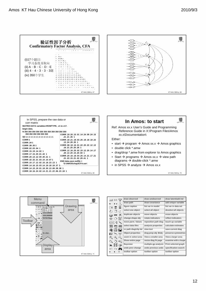
验证性因子分析验证性因子分析验证性因子分析验证性因子分析

(i)17个题目:学习态度及取向

(ii) A、B、C、D、E(iii) 4、4、3、3、3题

(iv) 350个学生

Confirmatory Factor Analysis, CFA

KT HAU SEM p. 68

In SPSS, prepare the raw data or corr matrix

MATRIX DATA variables=ROWTYPE_ v1 to v17.begin data.N 350 350 350 350 350 350 350 350 350 350 350

350 350 350 350 350 350SD 1 1 1 1 1 1 1 1 1 1 1 1 1 1 1 1 1 CORR 1CORR .34 1CORR .38 .35 1CORR .02 .03 .04 1CORR .15 .19 .14 .02 1CORR .17 .15 .20 .01 .42 1CORR .20 .13 .12 .00 .40 .21 1CORR .32 .32 .21 .03 .10 .10 .07 1CORR .10 .17 .12 .02 .15 .18 .23 .13 1CORR .14 .16 .15 .03 .14 .19 .18 .18 .37 1CORR .14 .15 .19 .01 .18 .30 .13 .08 .38 .38 1CORR .18 .16 .24 .02 .14 .21 .21 .22 .06 .23 .18 1

KT HAU SEM p. 69

CORR .19 .20 .15 .01 .14 .24 .09 .24 .15 .21 .21 .45 1

CORR .18 .21 .18 .03 .25 .18 .18 .18 .22 .12 .24 .28 .35 1

CORR .08 .18 .16 .01 .22 .20 .22 .12 .12 .16 .21 .25 .20 .26 1

CORR .12 .16 .25 .02 .15 .12 .20 .14 .17 .20 .14 .20 .15 .20 .50 1

CORR .20 .16 .18 .04 .25 .14 .21 .17 .21 .21 .23 .15 .21 .22 .29 .41 1

END data.save outfile = ‘D:\AMOS\chap3CFA.sav‘.

In Amos: to startRef: Amos xx.x User’s Guide and Programming

Reference Guide in X:\Program Files\Amos xx.x\Documentation\

Either:

• start � program � Amos xx.x � Amos graphics

• double click *.amw

• drag/drop *.amw from explorer to Amos graphics

• Start � programs � Amos xx.x � view path diagrams � double-click *.amw

• in SPSS � analyze � Amos xx.x

KT HAU SEM p. 70

KT HAU SEM p. 71

Menu command

Toolbar

Drawing area

Display area

KT HAU SEM p. 72

draw observed draw unobserved draw latent/add ind

draw path draw covariance add unique variable

figure caption list var in model list var in data set

select one object select all object deselect all objec ts

duplicate objects move objects erase objects

change shape obj rotate indicators reflect indicators

move parm. Values reposition path diag touch up variabl e

select data files analysis properties calculate estima tes

cc path diag/clip bd view text save current diag

Object properties drag prop obj ��obj preserve symmetries

zoom in select area View a smaller area View a larger area

Show entire page resize diag fit page examine with a lou pe

Bayesian multiple-gp analysis Print selected graph

undo prev change undo previous undo specification sear ch

toolbar option toolbar option toolbar option


13

KT HAU SEM p. 73

View input path diagram (model specification)

View output path diagram

Group numberModel selection

Unstandardized /standardized estimatesInteraction process

*.amw files

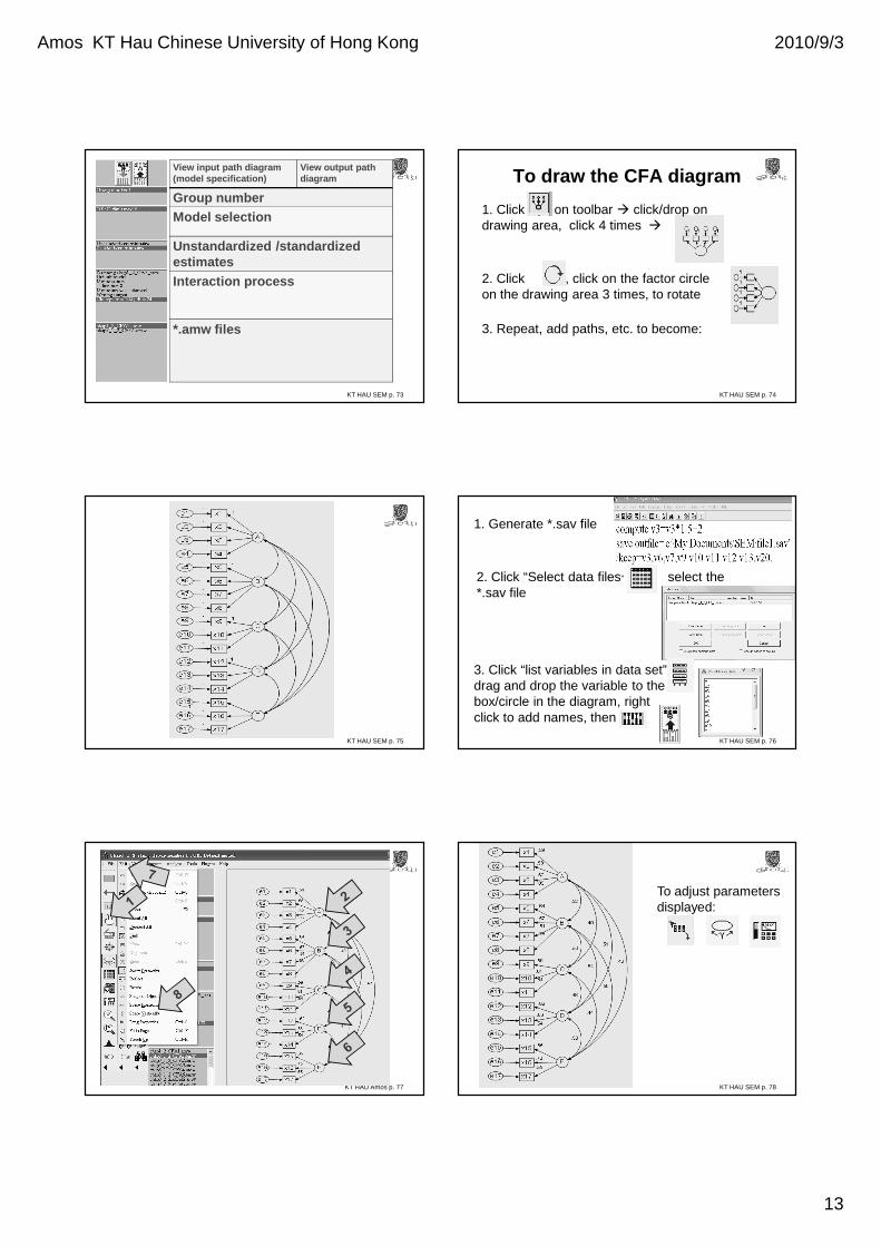
To draw the CFA diagram

KT HAU SEM p. 74

1. Click on toolbar � click/drop on drawing area, click 4 times �

2. Click , click on the factor circle on the drawing area 3 times, to rotate

3. Repeat, add paths, etc. to become:


2. Click “Select data files” select the *.sav file

3. Click “list variables in data set” drag and drop the variable to the box/circle in the diagram, right click to add names, then

1. Generate *.sav file

KT HAU Amos p. 77 KT HAU SEM p. 78

To adjust parameters displayed:


14

KT HAU SEM p. 79

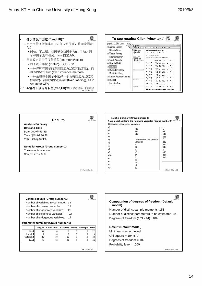
• 什么情况下固定什么情况下固定什么情况下固定什么情况下固定 (fixed, FI) ？？？？

– 两个变量（指标或因子）间没有关系，将元素固定为0

• 例如，不从属，将因子负荷固定为0。又如，因子和因子没有相关，固定为0。

– 需要设定因子的度量单位(set metric/scale)

• 因子没有单位 (metric)，无法计算。

• 一种将所有因子的方差固定为1(或其他常数)，简称为固定方差法 (fixed variance method)

• 一种是在每个因子中选择一个负荷固定为1(或其他常数)，简称为固定负荷法(fixed loading), as in Amos for CFA

• 什么情况下设定为自由什么情况下设定为自由什么情况下设定为自由什么情况下设定为自由(free,FR) :所有需要估计的参数KT HAU SEM p. 80

To see results: Click “view text”

KT HAU SEM p. 81

ResultsAnalysis SummaryDate and TimeDate: 2009年5月6日

Time: 下午 07:36:56Title Chap 3 CFA

Notes for Group (Group number 1)The model is recursiveSample size = 350

Variable Summary (Group number 1)Your model contains the following variables (Group number 1)Observed, endogenous variables

x1x2

x3x4x5

x6x7

x8x9x10

x11x12

x13x14

KT HAU SEM p. 82

x15x16x17

Unobserved, exogenous variablesAe1e2e3e4Be5e6e7e8

Ce9e10e11De12e13e14Ee15e16e17

KT HAU SEM p. 83

Variable counts (Group number 1)Number of variables in your model: 39Number of observed variables: 17Number of unobserved variables: 22Number of exogenous variables: 22Number of endogenous variables: 17

Weights Covariances Variances Means Intercepts Total

Fixed 22 0 0 0 0 22Labeled 0 0 0 0 0 0

Unlabeled 12 10 22 0 0 44

Total 34 10 22 0 0 66

Parameter summary (Group number 1)

Computation of degrees of freedom (Default model)

Number of distinct sample moments: 153

Number of distinct parameters to be estimated: 44

Degrees of freedom (153 - 44): 109

Result (Default model)Minimum was achieved

Chi-square = 194.570

Degrees of freedom = 109

Probability level = .000

KT HAU SEM p. 84


15

Standard Error SE参数参数参数参数 (parameter)

KT HAU SEM p. 85

Maximum Likelihood Estimates -- Regression Weights:

t-value=参数参数参数参数/SE=.980/.145=6.764Estimate S.E. C.R. P

x1 <--- A 1.000x2 <--- A .980 .145 6.764 ***x3 <--- A 1.050 .150 7.007 ***x4 <--- A .089 .110 .807 .419x5 <--- B 1.000x6 <--- B .888 .124 7.157 ***x7 <--- B .794 .115 6.881 ***x8 <--- B .436 .126 3.469 ***x9 <--- C 1.000x10 <--- C 1.045 .145 7.205 ***x11 <--- C 1.098 .152 7.229 ***x12 <--- D 1.000x13 <--- D 1.057 .132 8.032 ***x14 <--- D .875 .133 6.557 ***x15 <--- E 1.000x16 <--- E 1.100 .127 8.677 ***x17 <--- E .844 .119 7.087 ***

Standardized Regression Weights:

KT HAU SEM p. 86

Estimate

x1 <--- A .592x2 <--- A .580x3 <--- A .621x4 <--- A .053x5 <--- B .642x6 <--- B .571x7 <--- B .510x8 <--- B .280x9 <--- C .585x10 <--- C .612x11 <--- C .643x12 <--- D .621x13 <--- D .656x14 <--- D .543x15 <--- E .654x16 <--- E .719x17 <--- E .552

KT HAU SEM p. 87

Covariances: (Group number 1 - Default model)

Estimate S.E. C.R. PA <--> B .199 .040 4.934 ***A <--> C .139 .034 4.102 ***A <--> D .187 .039 4.798 ***A <--> E .163 .036 4.518 ***B <--> C .198 .039 5.096 ***B <--> D .215 .041 5.276 ***B <--> E .208 .042 4.895 ***C <--> D .174 .036 4.833 ***C <--> E .169 .037 4.573 ***D <--> E .201 .041 4.845 ***

KT HAU SEM p. 88

Correlations: (Group number 1 - Default model)

EstimateA <--> B .525A <--> C .402A <--> D .510A <--> E .423B <--> C .527B <--> D .541B <--> E .496C <--> D .481C <--> E .442D <--> E .496

KT HAU SEM p. 89

Variances: (Group number 1 - Default model)Estimate S.E. C.R. P

A .349 .074 4.725 ***B .411 .086 4.796 ***C .342 .072 4.774 ***D .384 .075 5.098 ***E .427 .077 5.562 ***e1 .648 .068 9.585 ***e2 .662 .068 9.808 ***e3 .612 .068 8.949 ***e4 .994 .075 13.192 ***e5 .586 .075 7.838 ***e6 .673 .067 10.034 ***e7 .738 .068 10.831 ***e8 .919 .074 12.398 ***e9 .656 .066 9.942 ***e10 .624 .066 9.397 ***e11 .585 .067 8.736 ***e12 .613 .065 9.363 ***e13 .568 .067 8.508 ***e14 .703 .067 10.512 ***e15 .570 .063 9.112 ***e16 .481 .065 7.382 ***e17 .693 .065 10.694 *** KT HAU SEM p. 90

Squared Multiple Correlations:

Estimatex17 .305x16 .518x15 .428x14 .295x13 .430x12 .385x11 .413x10 .374x9 .343x8 .078x7 .260x6 .325x5 .412x4 .003x3 .386x2 .336x1 .350


16

Modification Indices -- Covariances:

KT HAU SEM p. 91

M.I. Par Changee15 <--> e17 6.18 -.10e10 <--> e14 5.65 -.10e9 <--> e12 8.63 -.12e8 <--> D 6.57 .09e8 <--> B 16.58 -.15e8 <--> A 24.86 .17e7 <--> e13 5.77 -.10e7 <--> e9 4.33 .09e6 <--> e11 8.19 .12e6 <--> e7 5.92 -.10e5 <--> e8 5.34 -.10e5 <--> e7 5.86 .10e3 <--> e16 5.61 .09e2 <--> e8 10.38 .15e1 <--> e8 10.40 .15

Regression Weights:M.I.M.I.M.I.M.I. Par ChangePar ChangePar ChangePar Change

x17x17x17x17 <<<<------------ CCCC 4.384.384.384.38 .20.20.20.20

x17x17x17x17 <<<<------------ x5x5x5x5 4.284.284.284.28 .10.10.10.10

x16x16x16x16 <<<<------------ x11x11x11x11 4.254.254.254.25 ----.09.09.09.09

x16x16x16x16 <<<<------------ x6x6x6x6 4.174.174.174.17 ----.09.09.09.09

x16x16x16x16 <<<<------------ x5x5x5x5 4.054.054.054.05 ----.09.09.09.09

x14x14x14x14 <<<<------------ x9x9x9x9 4.064.064.064.06 .10.10.10.10

x14x14x14x14 <<<<------------ x5x5x5x5 4.374.374.374.37 .10.10.10.10

x13x13x13x13 <<<<------------ x7x7x7x7 5.825.825.825.82 ----.11.11.11.11

x12x12x12x12 <<<<------------ x9x9x9x9 6.256.256.256.25 ----.12.12.12.12

x11x11x11x11 <<<<------------ x6x6x6x6 5.225.225.225.22 .11.11.11.11

x9x9x9x9 <<<<------------ x12x12x12x12 6.686.686.686.68 ----.12.12.12.12

x8x8x8x8 <<<<------------ DDDD 10.4010.4010.4010.40 .32.32.32.32

x8x8x8x8 <<<<------------ AAAA 20.6120.6120.6120.61 .49.49.49.49x8x8x8x8 <<<<------------ x13x13x13x13 8.728.728.728.72 .15.15.15.15

x8x8x8x8 <<<<------------ x12x12x12x12 6.256.256.256.25 .13.13.13.13

x8x8x8x8 <<<<------------ x3x3x3x3 5.885.885.885.88 .13.13.13.13

x8x8x8x8 <<<<------------ x2x2x2x2 20.8320.8320.8320.83 .24.24.24.24

x8x8x8x8 <<<<------------ x1x1x1x1 20.9020.9020.9020.90 .24.24.24.24

x6x6x6x6 <<<<------------ x11x11x11x11 6.406.406.406.40 .12.12.12.12

x5x5x5x5 <<<<------------ x12x12x12x12 4.144.144.144.14 ----.09.09.09.09

x5x5x5x5 <<<<------------ x8x8x8x8 4.834.834.834.83 ----.10.10.10.10

x2x2x2x2 <<<<------------ x8x8x8x8 9.859.859.859.85 .15.15.15.15

x1x1x1x1 <<<<------------ x8x8x8x8 9.549.549.549.54 .15.15.15.15KT HAU SEM p. 92

Maximum Modification Index is 20.61 for Element x8 A修正指数:该参数由固定改为自由估计改为自由估计改为自由估计改为自由估计，，，，会减少会减少会减少会减少的数值的数值的数值的数值

Minimization History (Default model)Iterat-

ion- veEV

Condition #Smallest

EVDiameter F

N Tries

Ratio

0 e 13 -.16 9999.00 1310.09 0 9999.001 e 0 83.44 2.15 390.84 20 .752 e 0 28.83 .67 308.08 5 .003 e 0 35.91 .80 219.15 2 .004 e 0 70.96 .55 196.21 1 .985 e 0 89.24 .16 194.60 1 .996 e 0 92.32 .02 194.57 1 1.017 e 0 91.81 .00 194.57 1 1.00

KT HAU SEM p. 93

Sat. nPar = p x (p+1)/2Ind. nPar = p

0.56 x (N-1) = chi0.56x349=194.57

KT HAU SEM p. 94

Model Fit Summary 拟合优度统计拟合优度统计拟合优度统计拟合优度统计量量量量

Model NPAR CMIN DF P CMIN/DF

Default model 44 194.57 109 .00 1.79Saturated model 153 .00 0Independence model 17 1104.79 136 .00 8.12

Model RMR GFI AGFI PGFI

Default model .05 .94 .92 .67Saturated model .00 1.00Independence model .19 .60 .55 .53

Oldest (LISREL) indexes: RMR, GFI, AGFI, (SRMR)

pRatio = df (hypo model)/df (null model)= (153 - 44) / (153-17)= 109 / 136 = 0.801

KT HAU SEM p. 95

TLI = NNFI CFI = RNI

ModelNFI

Delta1RFI

rho1IFI

Delta2TLI

rho2CFI

Default model .82 .78 .91 .89 .91Saturated model 1.00 1.00 1.00Independence model .00 .00 .00 .00 .00

Model PRATIO PNFI PCFI

Default model .80 .66 .73

Saturated model .00 .00 .00Independence model 1.00 .00 .00

PCFI = pRatio x CFI= .80 x .91= .73

0.56 x (N-1) = CMin0.56x349=194.57

CMin – df = 194.57 - 109

Model NCP LO 90 HI 90Default model 85.57 50.51 128.48Saturated model .00 .00 .00Independence model 968.79 866.55 1078.48

KT HAU SEM p. 96

Lo – Hi =confidence interval

Model FMIN F0 LO 90 HI 90Default model .56 .25 .14 .37Saturated model .00 .00 .00 .00Independence model 3.17 2.78 2.48 3.09

Model RMSEA LO 90 HI 90 PCLOSE

Default model .05 .04 .06 .64Independence model .14 .14 .15 .00


17

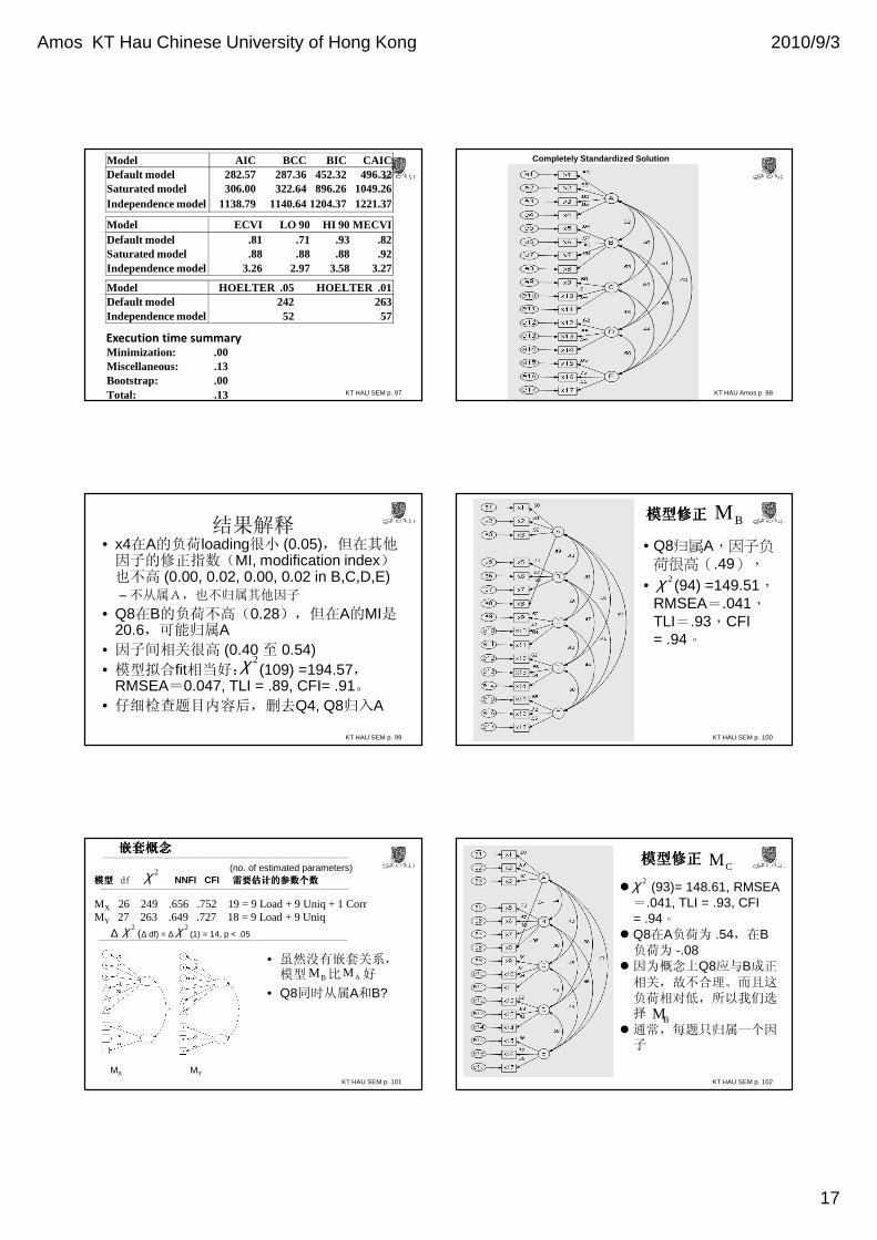
Model AIC BCC BIC CAICDefault model 282.57 287.36 452.32 496.32Saturated model 306.00 322.64 896.26 1049.26Independence model 1138.79 1140.64 1204.37 1221.37

KT HAU SEM p. 97

Model ECVI LO 90 HI 90 MECVIDefault model .81 .71 .93 .82Saturated model .88 .88 .88 .92Independence model 3.26 2.97 3.58 3.27

Model HOELTER .05 HOELTER .01Default model 242 263Independence model 52 57

Minimization: .00Miscellaneous: .13Bootstrap: .00Total: .13

Execution time summary

KT HAU Amos p. 98

Completely Standardized Solution

KT HAU SEM p. 99

结果解释• x4在A的负荷loading很小 (0.05)，但在其他因子的修正指数（MI, modification index）也不高 (0.00, 0.02, 0.00, 0.02 in B,C,D,E)– 不从属Ａ，也不归属其他因子

• Q8在B的负荷不高（0.28），但在A的MI是20.6，可能归属A

• 因子间相关很高 (0.40 至 0.54)• 模型拟合fit相当好： (109) =194.57，

RMSEA＝0.047, TLI = .89, CFI= .91。• 仔细检查题目内容后，删去Q4, Q8归入A

2χ

KT HAU SEM p. 100

2χ

• Q8归属A，因子负荷很高（.49），

• (94) =149.51，RMSEA＝.041，TLI＝.93，CFI = .94。

模型修正模型修正模型修正模型修正 BM

KT HAU SEM p. 101

• 虽然没有嵌套关系，模型比好

• Q8同时从属A和B?

_______________________________________________________________________________________

(no. of estimated parameters)模型模型模型模型 df NNFI CFI 需要估计的参数个数需要估计的参数个数需要估计的参数个数需要估计的参数个数________________________________________________________________________________________

MX 26 249 .656 .752 19 = 9 Load + 9 Uniq + 1 CorrMY 27 263 .649 .727 18 = 9 Load + 9 Uniq

________________________________________________________________________________________∆ (∆ df) = ∆ (1) = 14, p < .052χ 2χ

BM AM

MX MY

嵌套概念嵌套概念嵌套概念嵌套概念

2χ

KT HAU SEM p. 102

模型修正模型修正模型修正模型修正CM

� (93)= 148.61, RMSEA＝.041, TLI = .93, CFI = .94。

� Q8在A负荷为 .54，在B负荷为 -.08

� 因为概念上Q8应与B成正相关，故不合理。而且这负荷相对低，所以我们选择

� 通常，每题只归属一个因子

2χ

BM


18

KT HAU SEM p. 103

修正修正修正修正modification 前后模型的拟合指数比较前后模型的拟合指数比较前后模型的拟合指数比较前后模型的拟合指数比较

______________________________________

模型 df RMSEA NNFI CFI 註______________________________________

M-A 109 195 .046 .89 .91 原模型

M-B 94 150 .041 .93 .94 删Q4,Q8-AM-C 93 149 .041 .93 .94 删Q4,Q8-A,BMB-2 99 152 .039 .94 .95 2阶因子______________________________________

2χ

KT HAU SEM p. 104


V 多质多法模型多质多法模型多质多法模型多质多法模型V multitrait-multimethod

(MTMM)




KT HAU SEM p. 105

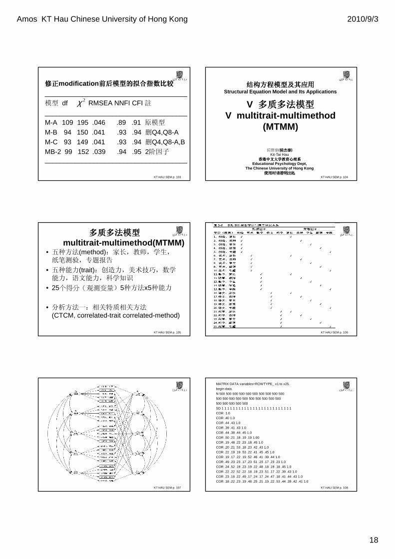
多质多法模型多质多法模型多质多法模型多质多法模型multitrait-multimethod(MTMM)

• 五种方法(method)：家长，教师，学生，纸笔测验，专题报告

• 五种能力(trait)：创造力，美术技巧，数学能力，语文能力，科学知识

• 25个得分（观测变量）5种方法x5种能力

• 分析方法一：相关特质相关方法(CTCM, correlated-trait correlated-method)

KT HAU SEM p. 106

KT HAU SEM p. 107

MATRIX DATA variables=ROWTYPE_ x1 to x25.

begin data.

N 500 500 500 500 500 500 500 500 500 500

500 500 500 500 500 500 500 500 500 500

500 500 500 500 500

SD 1 1 1 1 1 1 1 1 1 1 1 1 1 1 1 1 1 1 1 1 1 1 1 1 1

COR 1.0

COR .40 1.0

COR .44 .43 1.0

COR .39 .41 .43 1.0

COR .44 .38 .44 .45 1.0

COR .50 .21 .18 .19 .19 1.00

COR .19 .48 .22 .23 .18 .45 1.0

COR .20 .21 .53 .18 .23 .42 .43 1.0

COR .22 .19 .19 .53 .22 .41 .45 .45 1.0

COR .19 .17 .22 .19 .52 .46 .41 .39 .44 1.0

COR .49 .23 .23 .17 .23 .51 .23 .17 .23 .23 1.0

COR .24 .52 .19 .23 .19 .22 .48 .18 .19 .18 .45 1.0

COR .22 .22 .52 .22 .18 .19 .23 .51 .17 .22 .39 .43 1.0

COR .23 .18 .22 .49 .17 .24 .17 .24 .47 .18 .41 .44 .43 1.0

COR .18 .22 .23 .19 .48 .25 .21 .19 .22 .53 .44 .39 .42 .41 1.0

KT HAU SEM p. 108


19

KT HAU SEM p. 109

COR .48 .23 .18 .23 .23 .48 .18 .23 .25 .24 .55 .23 .19 .24 .23 1.0

COR .22 .51 .17 .19 .21 .19 .51 .19 .23 .23 .23 .52 .23 .19 .17 .43 1.0

COR .23 .22 .48 .22 .19 .23 .23 .53 .23 .22 .24 .22 .47 .22 .19 .45 .39 1.0

COR .19 .23 .23 .53 .22 .24 .19 .24 .53 .19 .21 .24 .23 .48 .23 .42 .46 .45 1.0

COR .20 .24 .17 .23 .49 .21 .16 .19 .19 .51 .24 .18 .24 .22 .52 .41 .43 .39 .45 1.0

COR .51 .22 .18 .19 .18 .52 .25 .24 .24 .23 .49 .24 .21 .24 .24 .53 .24 .23 .23 .24 1.0

COR .22 .53 .23 .18 .17 .25 .53 .17 .18 .24 .19 .52 .18 .19 .17 .24 .49 .19 .21 .21 .45 1.0

COR .19 .22 .47 .22 .23 .22 .23 .47 .17 .17 .23 .22 .47 .21 .24 .23 .23 .53 .24 .23 .41 .45 1.0

COR .22 .23 .22 .52 .21 .19 .17 .24 .53 .19 .19 .19 .18 .53 .22 .19 .21 .18 .51 .18 .43 .41 .45 1.0

COR .20 .24 .19 .19 .49 .18 .19 .19 .23 .52 .23 .17 .23 .19 .52 .24 .18 .24 .17 .25 .44 .42 .43 .41 1.0

END data.

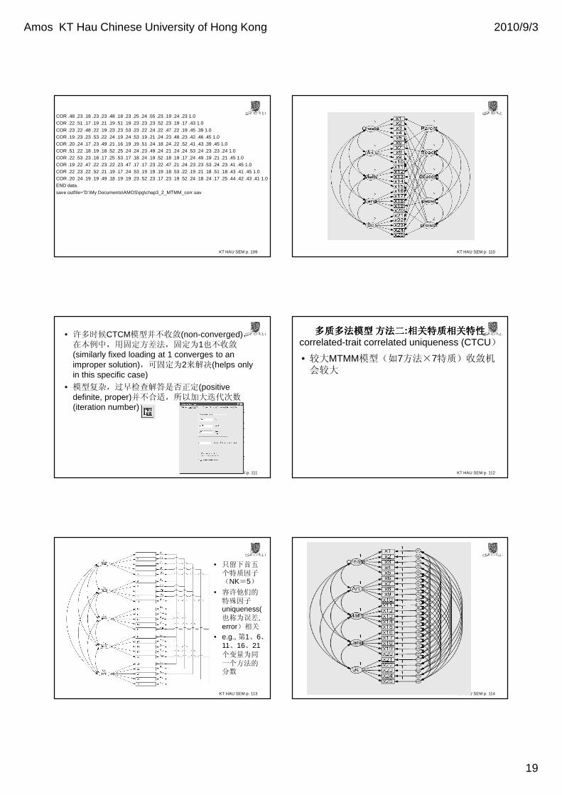
save outfile='D:\My Documents\AMOS\pg\chap3_2_MTMM_corr.sav

KT HAU SEM p. 110

KT HAU SEM p. 111

• 许多时候CTCM模型并不收敛(non-converged)，在本例中，用固定方差法，固定为1也不收敛(similarly fixed loading at 1 converges to an improper solution)，可固定为2来解决(helps only in this specific case)

• 模型复杂，过早检查解答是否正定(positive definite, proper)并不合适，所以加大迭代次数(iteration number)

KT HAU SEM p. 112

多质多法模型多质多法模型多质多法模型多质多法模型方法二方法二方法二方法二:相关特质相关特性相关特质相关特性相关特质相关特性相关特质相关特性correlated-trait correlated uniqueness (CTCU）

• 较大MTMM模型（如7方法×7特质）收敛机会较大

KT HAU SEM p. 113

• 只留下首五个特质因子（NK＝5）

• 容许他们的特殊因子uniqueness(也称为误差, error）相关

• e.g., 第1、6、11、16、21个变量为同一个方法的分数

KT HAU SEM p. 114


20

Checking• proper solutions

• fit reasonably well

• assuming all items are correctly oriented (all +ve related), then

– in CTCM: all trait and method effect loadings� all +ve;

– in CTCU: all trait method loadings +ve; all CU +ve/zero

– correlations among traits or among methods: depend on theory



VI 全模型全模型全模型全模型

VI Full model




KT HAU SEM p. 117

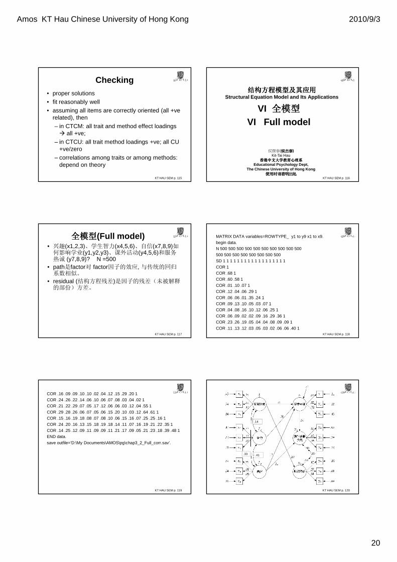
全模型全模型全模型全模型(Full model)• 兴趣(x1,2,3)、学生智力(x4,5,6)、自信(x7,8,9)如何影响学业(y1,y2,y3)、课外活动(y4,5,6)和服务热诚 (y7,8,9)? N =500

• path是factor对 factor因子的效应, 与传统的回归系数相似。

• residual (结构方程残差)是因子的残差（未被解释的部份）方差。

MATRIX DATA variables=ROWTYPE_ y1 to y9 x1 to x9.begin data.N 500 500 500 500 500 500 500 500 500 500

500 500 500 500 500 500 500 500SD 1 1 1 1 1 1 1 1 1 1 1 1 1 1 1 1 1 1

COR 1COR .68 1COR .60 .58 1

COR .01 .10 .07 1COR .12 .04 .06 .29 1

COR .06 .06 .01 .35 .24 1COR .09 .13 .10 .05 .03 .07 1COR .04 .08 .16 .10 .12 .06 .25 1

COR .06 .09 .02 .02 .09 .16 .29 .36 1COR .23 .26 .19 .05 .04 .04 .08 .09 .09 1

COR .11 .13 .12 .03 .05 .03 .02 .06 .06 .40 1KT HAU SEM p. 118

COR .16 .09 .09 .10 .10 .02 .04 .12 .15 .29 .20 1COR .24 .26 .22 .14 .06 .10 .06 .07 .08 .03 .04 .02 1COR .21 .22 .29 .07 .05 .17 .12 .06 .06 .03 .12 .04 .55 1

COR .29 .28 .26 .06 .07 .05 .06 .15 .20 .10 .03 .12 .64 .61 1COR .15 .16 .19 .18 .08 .07 .08 .10 .06 .15 .16 .07 .25 .25 .16 1

COR .24 .20 .16 .13 .15 .18 .19 .18 .14 .11 .07 .16 .19 .21 .22 .35 1COR .14 .25 .12 .09 .11 .09 .09 .11 .21 .17 .09 .05 .21 .23 .18 .39 .48 1END data.

save outfile='D:\My Documents\AMOS\pg\chap3_2_Full_corr.sav'.


.14

.33 .41


21

KT HAU SEM p. 121

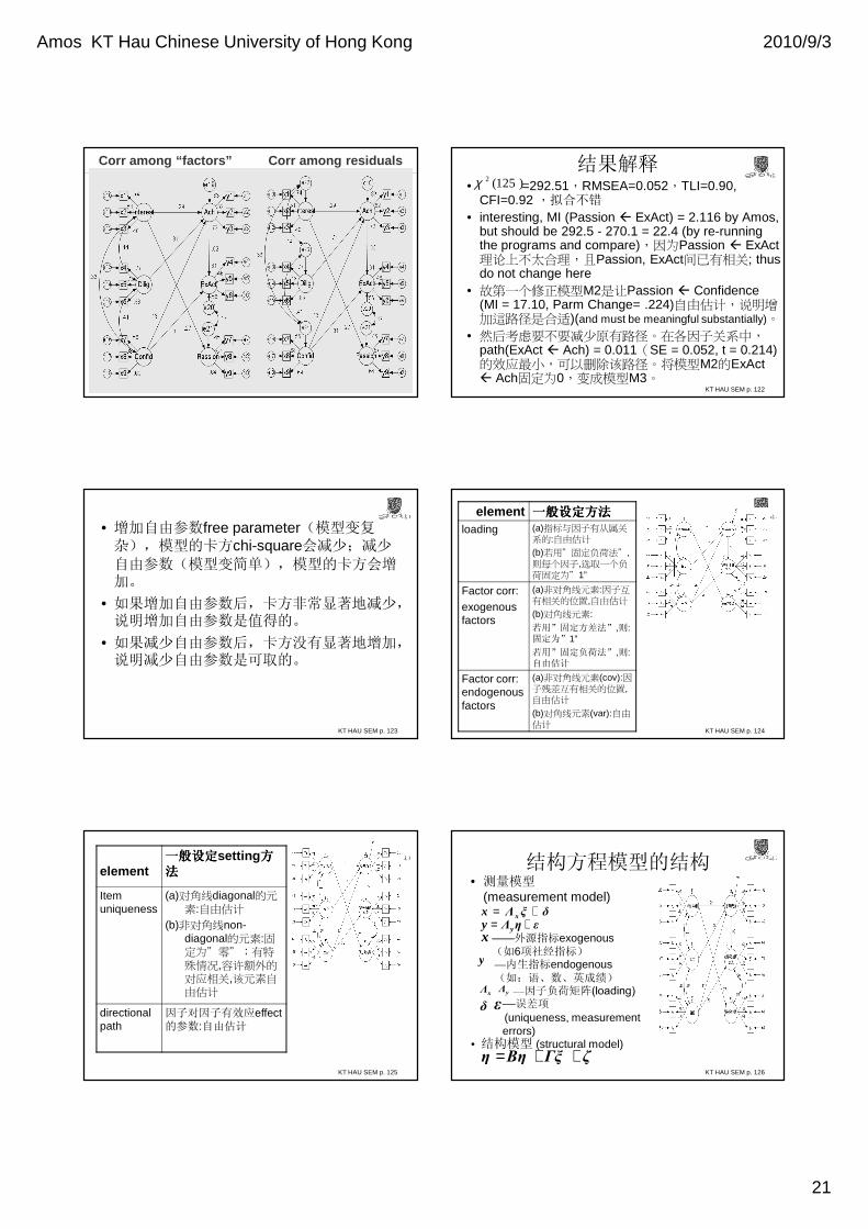
Corr among “factors” Corr among residuals

KT HAU SEM p. 122

结果解释• =292.51，RMSEA=0.052，TLI=0.90,

CFI=0.92 ，拟合不错

• interesting, MI (Passion ExAct) = 2.116 by Amos, but should be 292.5 - 270.1 = 22.4 (by re-running the programs and compare)，因为Passion ExAct 理论上不太合理，且Passion, ExAct间已有相关; thus do not change here

• 故第一个修正模型M2是让Passion Confidence (MI = 17.10, Parm Change= .224)自由估计，说明增加這路径是合适)(and must be meaningful substantially)。

• 然后考虑要不要减少原有路径。在各因子关系中，path(ExAct Ach) = 0.011（SE = 0.052, t = 0.214)的效应最小，可以删除该路径。将模型M2的ExAct Ach固定为0，变成模型M3。

)125(2χ

KT HAU SEM p. 123

• 增加自由参数free parameter（模型变复杂），模型的卡方chi-square会减少；减少

自由参数（模型变简单），模型的卡方会增加。

• 如果增加自由参数后，卡方非常显著地减少，说明增加自由参数是值得的。

• 如果减少自由参数后，卡方没有显著地增加，说明减少自由参数是可取的。

KT HAU SEM p. 124

element 一般设定方法一般设定方法一般设定方法一般设定方法

loading (a)指标与因子有从属关系的:自由估计

(b)若用”固定负荷法”,则每个因子,选取一个负荷固定为”1”

Factor corr:exogenous factors

(a)非对角线元素:因子互有相关的位置,自由估计

(b)对角线元素:

若用”固定方差法”,则: 固定为”1”

若用”固定负荷法”,则:自由估计

Factor corr: endogenous factors

(a)非对角线元素(cov):因子残差互有相关的位置,自由估计

(b)对角线元素(var):自由估计

KT HAU SEM p. 125

element一般设定一般设定一般设定一般设定setting 方方方方法法法法

Item uniqueness

(a)对角线diagonal的元素:自由估计

(b)非对角线non-diagonal的元素:固定为”零”；有特殊情况,容许额外的对应相关,该元素自由估计

directional path

因子对因子有效应effect的参数:自由估计

KT HAU SEM p. 126

结构方程模型的结构• 测量模型

(measurement model)δξΛx x +=εηΛy y +=

x ——外源指标exogenous（如6项社经指标）

y —内生指标endogenous（如：语、数、英成绩）

xΛ yΛ

δ ε—误差项(uniqueness, measurement errors)

• 结构模型 (structural model)ζΓξΒηη ++=


22

KT HAU SEM p. 127


VII 高高高高阶阶阶阶因子分析因子分析因子分析因子分析VII High-order Factor Analysis




KT HAU SEM p. 128

高高高高阶阶阶阶因子分析因子分析因子分析因子分析(high-order factor analysis)

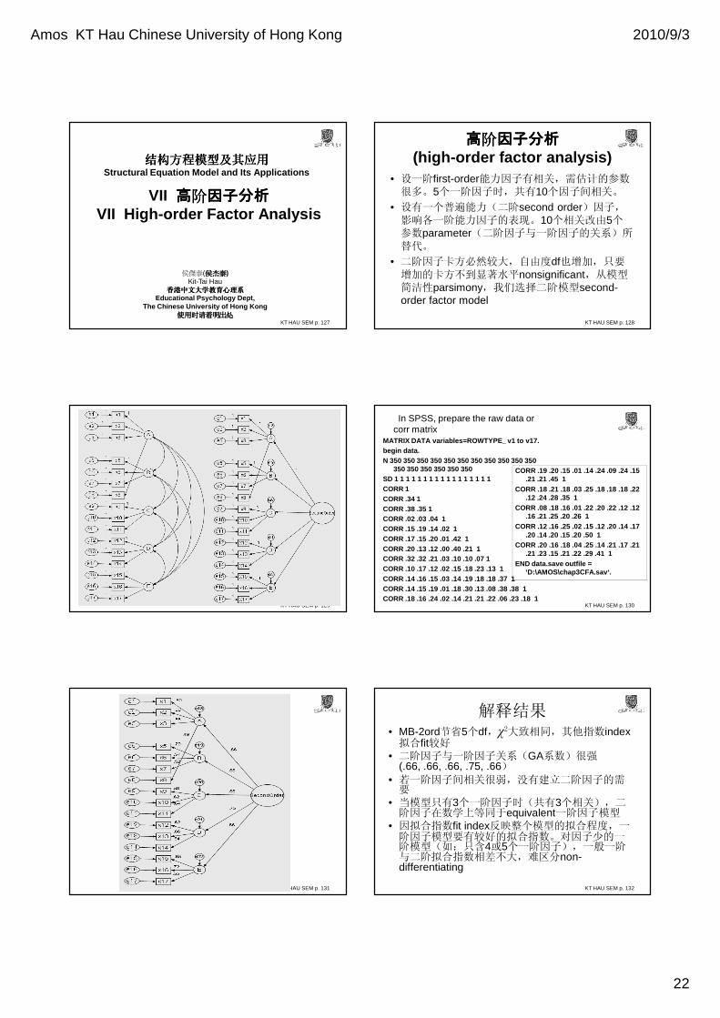
• 设一阶first-order能力因子有相关，需估计的参数很多。5个一阶因子时，共有10个因子间相关。

• 设有一个普遍能力（二阶second order）因子，影响各一阶能力因子的表现。10个相关改由5个参数parameter（二阶因子与一阶因子的关系）所替代。

• 二阶因子卡方必然较大，自由度df也增加，只要增加的卡方不到显著水平nonsignificant，从模型简洁性parsimony，我们选择二阶模型second-order factor model

KT HAU SEM p. 129

In SPSS, prepare the raw data or corr matrix

MATRIX DATA variables=ROWTYPE_ v1 to v17.begin data.N 350 350 350 350 350 350 350 350 350 350 350

350 350 350 350 350 350SD 1 1 1 1 1 1 1 1 1 1 1 1 1 1 1 1 1 CORR 1CORR .34 1CORR .38 .35 1CORR .02 .03 .04 1CORR .15 .19 .14 .02 1CORR .17 .15 .20 .01 .42 1CORR .20 .13 .12 .00 .40 .21 1CORR .32 .32 .21 .03 .10 .10 .07 1CORR .10 .17 .12 .02 .15 .18 .23 .13 1CORR .14 .16 .15 .03 .14 .19 .18 .18 .37 1CORR .14 .15 .19 .01 .18 .30 .13 .08 .38 .38 1CORR .18 .16 .24 .02 .14 .21 .21 .22 .06 .23 .18 1

KT HAU SEM p. 130

CORR .19 .20 .15 .01 .14 .24 .09 .24 .15 .21 .21 .45 1

CORR .18 .21 .18 .03 .25 .18 .18 .18 .22 .12 .24 .28 .35 1

CORR .08 .18 .16 .01 .22 .20 .22 .12 .12 .16 .21 .25 .20 .26 1

CORR .12 .16 .25 .02 .15 .12 .20 .14 .17 .20 .14 .20 .15 .20 .50 1

CORR .20 .16 .18 .04 .25 .14 .21 .17 .21 .21 .23 .15 .21 .22 .29 .41 1

END data.save outfile = ‘D:\AMOS\chap3CFA.sav‘.


解释结果• MB-2ord节省5个df，χ2大致相同，其他指数index拟合fit较好

• 二阶因子与一阶因子关系（GA系数）很强(.66, .66, .66, .75, .66）

• 若一阶因子间相关很弱，没有建立二阶因子的需要

• 当模型只有3个一阶因子时（共有3个相关），二阶因子在数学上等同于equivalent一阶因子模型

• 因拟合指数fit index反映整个模型的拟合程度，一阶因子模型要有较好的拟合指数。对因子少的一阶模型（如：只含4或5个一阶因子），一般一阶与二阶拟合指数相差不大，难区分non-differentiating


23

KT HAU SEM p. 133

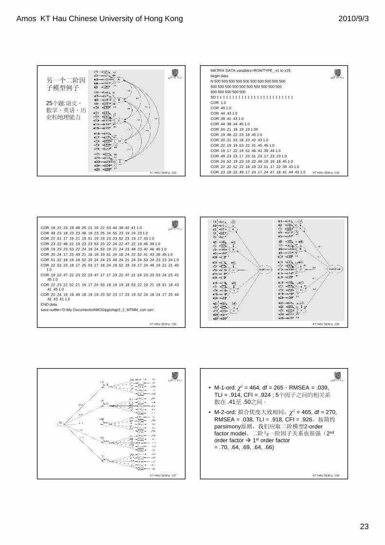
另一个二阶因子模型例子

25个题:语文、数学、英语、历史和地理能力

MATRIX DATA variables=ROWTYPE_ x1 to x25.begin data.N 500 500 500 500 500 500 500 500 500 500500 500 500 500 500 500 500 500 500 500500 500 500 500 500SD 1 1 1 1 1 1 1 1 1 1 1 1 1 1 1 1 1 1 1 1 1 1 1 1 1 COR 1.0COR .40 1.0COR .44 .43 1.0COR .39 .41 .43 1.0 COR .44 .38 .44 .45 1.0COR .50 .21 .18 .19 .19 1.00COR .19 .48 .22 .23 .18 .45 1.0COR .20 .21 .53 .18 .23 .42 .43 1.0COR .22 .19 .19 .53 .22 .41 .45 .45 1.0COR .19 .17 .22 .19 .52 .46 .41 .39 .44 1.0COR .49 .23 .23 .17 .23 .51 .23 .17 .23 .23 1.0COR .24 .52 .19 .23 .19 .22 .48 .18 .19 .18 .45 1.0COR .22 .22 .52 .22 .18 .19 .23 .51 .17 .22 .39 .43 1.0COR .23 .18 .22 .49 .17 .24 .17 .24 .47 .18 .41 .44 .43 1.0 KT HAU SEM p. 134

COR .18 .22 .23 .19 .48 .25 .21 .19 .22 .53 .44 .39 .42 .41 1.0COR .48 .23 .18 .23 .23 .48 .18 .23 .25 .24 .55 .23 .19 .24 .23 1.0COR .22 .51 .17 .19 .21 .19 .51 .19 .23 .23 .23 .52 .23 .19 .17 .43 1.0COR .23 .22 .48 .22 .19 .23 .23 .53 .23 .22 .24 .22 .47 .22 .19 .45 .39 1.0 COR .19 .23 .23 .53 .22 .24 .19 .24 .53 .19 .21 .24 .23 .48 .23 .42 .46 .45 1.0COR .20 .24 .17 .23 .49 .21 .16 .19 .19 .51 .24 .18 .24 .22 .52 .41 .43 .39 .45 1.0COR .51 .22 .18 .19 .18 .52 .25 .24 .24 .23 .49 .24 .21 .24 .24 .53 .24 .23 .23 .24 1.0 COR .22 .53 .23 .18 .17 .25 .53 .17 .18 .24 .19 .52 .18 .19 .17 .24 .49 .19 .21 .21 .45

1.0COR .19 .22 .47 .22 .23 .22 .23 .47 .17 .17 .23 .22 .47 .21 .24 .23 .23 .53 .24 .23 .41

.45 1.0 COR .22 .23 .22 .52 .21 .19 .17 .24 .53 .19 .19 .19 .18 .53 .22 .19 .21 .18 .51 .18 .43

.41 .45 1.0COR .20 .24 .19 .19 .49 .18 .19 .19 .23 .52 .23 .17 .23 .19 .52 .24 .18 .24 .17 .25 .44

.42 .43 .41 1.0 END data.save outfile='D:\My Documents\AMOS\pg\chap3_2_MTMM_corr.sav'.



• M-1-ord: χ2 = 464, df = 265，RMSEA = .039, TLI = .914, CFI = .924 ; 5个因子之间的相关系数在 .41至 .50之间。

• M-2-ord: 拟合优度大致相同，χ2 = 465, df = 270, RMSEA = .038, TLI = .918, CFI = .926。按简约parsimony原则，我们应取二阶模型2-order factor model。二阶与一阶因子关系也很强（2nd

order factor � 1st order factor= .70, .64, .69, .64, .66)


24

KT HAU SEM p. 139

一般在二阶因子模型中一般在二阶因子模型中一般在二阶因子模型中一般在二阶因子模型中：：：：• 一阶因子间一阶因子间一阶因子间一阶因子间不再容许相关不再容许相关不再容许相关不再容许相关• 二阶与一阶因子间路径二阶与一阶因子间路径二阶与一阶因子间路径二阶与一阶因子间路径:方向是方向是方向是方向是由二由二由二由二

阶至一阶阶至一阶阶至一阶阶至一阶• 二阶与一阶因子各路径中二阶与一阶因子各路径中二阶与一阶因子各路径中二阶与一阶因子各路径中, 我们取我们取我们取我们取其其其其

中一个固定为中一个固定为中一个固定为中一个固定为1(固定负荷法固定负荷法固定负荷法固定负荷法)• 对只有对只有对只有对只有3个或以下个或以下个或以下个或以下一阶因子一阶因子一阶因子一阶因子,不再构划不再构划不再构划不再构划

二阶因子二阶因子二阶因子二阶因子• 何时宁取二阶模型何时宁取二阶模型何时宁取二阶模型何时宁取二阶模型，，，，要考虑要考虑要考虑要考虑：：：：

– 二阶二阶二阶二阶自由度较对应一阶模型为大自由度较对应一阶模型为大自由度较对应一阶模型为大自由度较对应一阶模型为大

– 二阶模型较对应一阶模型二阶模型较对应一阶模型二阶模型较对应一阶模型二阶模型较对应一阶模型简单简单简单简单(parsimonious)

– 二阶的二阶的二阶的二阶的χχχχ2较一阶为大较一阶为大较一阶为大较一阶为大– 若二阶模型简化甚多若二阶模型简化甚多若二阶模型简化甚多若二阶模型简化甚多，，，，但但但但χχχχ2增加增加增加增加

不多不多不多不多(模型拟合恶化不严重模型拟合恶化不严重模型拟合恶化不严重模型拟合恶化不严重），），），），则则则则宁取二阶模型宁取二阶模型宁取二阶模型宁取二阶模型

• 在在在在LISREL中设定高阶因子中设定高阶因子中设定高阶因子中设定高阶因子,可可可可– 二阶因子用二阶因子用二阶因子用二阶因子用ξξξξ ,一阶因子用一阶因子用一阶因子用一阶因子用ηηηη代表代表代表代表– 二阶与一阶因子均用二阶与一阶因子均用二阶与一阶因子均用二阶与一阶因子均用ηηηη代表代表代表代表 KT HAU SEM p. 140


VIII 单纯形模型单纯形模型单纯形模型单纯形模型

VIII simplex model




KT HAU SEM p. 141

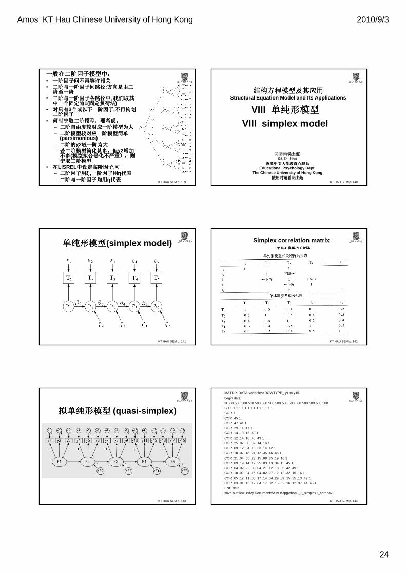
单纯形模型单纯形模型单纯形模型单纯形模型(simplex model)

KT HAU SEM p. 142

Simplex correlation matrix

KT HAU SEM p. 143

拟单纯形模型拟单纯形模型拟单纯形模型拟单纯形模型 (quasi-simplex)

MATRIX DATA variables=ROWTYPE_ y1 to y15.

begin data.

N 500 500 500 500 500 500 500 500 500 500 500 500 500 500 500

SD 1 1 1 1 1 1 1 1 1 1 1 1 1 1 1

COR 1

COR .45 1

COR .47 .41 1

COR .29 .11 .17 1

COR .14 .19 .13 .49 1

COR .12 .14 .18 .46 .43 1

COR .25 .07 .08 .32 .14 .16 1

COR .09 .12 .04 .15 .33 .14 .42 1

COR .10 .07 .18 .24 .12 .35 .46 .45 1

COR .21 .04 .05 .23 .15 .08 .35 .19 .16 1

COR .09 .19 .14 .12 .25 .03 .13 .34 .15 .45 1

COR .04 .02 .22 .09 .04 .21 .12 .18 .35 .42 .49 1

COR .18 .02 .04 .16 .04 .02 .27 .12 .12 .32 .15 .16 1

COR .05 .12 .11 .05 .17 .14 .04 .29 .09 .15 .35 .13 .49 1

COR .03 .01 .13 .12 .04 .17 .02 .15 .32 .16 .12 .37 .44 .45 1

END data.

save outfile='D:\My Documents\AMOS\pg\chap3_2_simplex1_corr.sav'.

KT HAU SEM p. 144


25



KT HAU SEM p. 149

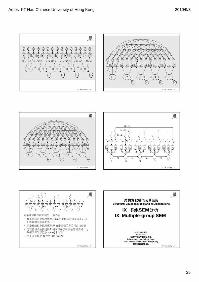
对单纯或拟单纯形模型,一般而言

• 对单指标的单纯型模型, 首尾两个指标的误差方差，我们需强制为零或相等

• 多指标的拟单纯形模型,所有指针误差方差可自由估计

• 用误差相关去描述跨年相同对应学科误差的相关时，这些相关应为正值(positive)才合理

• 加了误差相关,模式的自由度减少

KT HAU SEM p. 150


IX 多组多组多组多组SEM分析分析分析分析IX Multiple-group SEM





26

KT HAU SEM p. 151

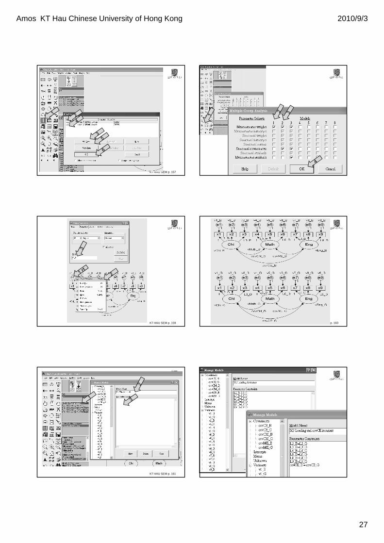
多组多组多组多组SEM分析分析分析分析

(multiple-group SEM)• 第一类:多组验证性因子分析multiple-group CFA（或路径分析path analyses）– 各组（例如男、女组）的因子结构factor

structure是否相同？某些路径path参数parameter/coefficient在不同的组是否有显著差异significant difference？(与比较多组回归系数regression coefficients in multiple group是否相同类似)

• 第二类:各组的因子均值是否相同(Multiple-group Mean Structure Analysis)。这与传统方差分析ANOVA相似 (通常需要先做第一类分析)

KT HAU SEM p. 152

多组验证性因子分析多组验证性因子分析多组验证性因子分析多组验证性因子分析multiple-group CFA

1. 形态相同（configural/pattern invariance）

2. 因子负荷factor loading LX等同invariance3. 误差方差uniqueness TD等同invariance4. 因子方差factor variance, diagonal of PH

等同invariance

5. 因子协方差factor covariance PH 等同invariance

KT HAU SEM p. 153

表表表表4-2 多组验证性因子分析各模型的拟合指数多组验证性因子分析各模型的拟合指数多组验证性因子分析各模型的拟合指数多组验证性因子分析各模型的拟合指数Model df chi-2 RMSEA TLI CFIM0,M男生单独估计 24 49.57 .042 .966 .977M0,F女生单独估计 24 44.93 .035 .974 .982M1 两组同时估计, no Inv 48 94.50 .027 .970 .980M2 Loading Inv 54 107.19 .028 .969 .977M3 Ld, PH(3,1) Inv 55 107.52 .027 .970 .977M4 Ld, FacCov Inv 60 109.32 .025 .974 .979M5 Ld、FacCov、U Inv 69 131.21 .026 .972 .973M7 Ld,FacCov,U,Intrcpt Inv;

Fac meanFree 75 132.23 .024 .976 .975M8 Ld,FacCov,U,Intrcpt,

Fac mean Inv 78 146.80 .026 .973 .970

KT HAU SEM p. 154

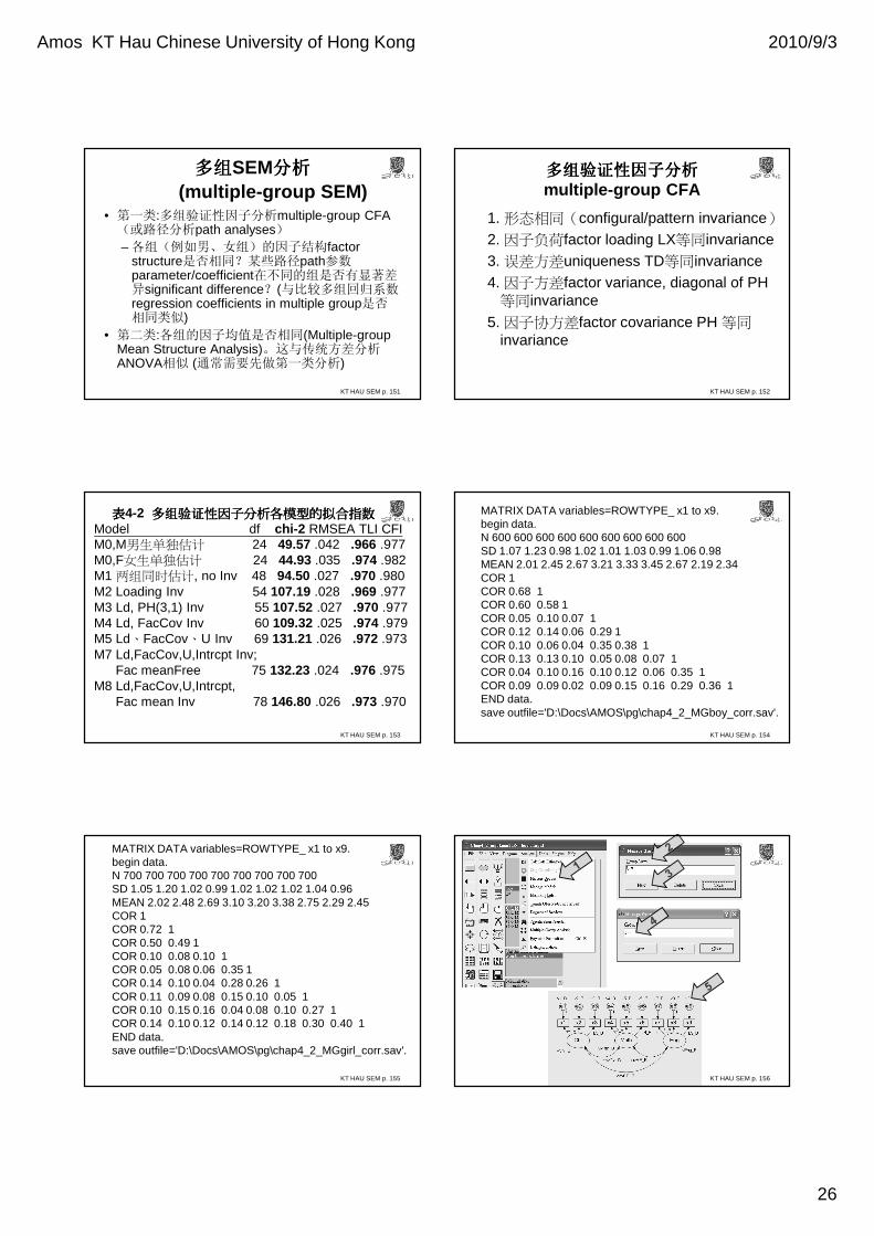
MATRIX DATA variables=ROWTYPE_ x1 to x9.begin data.N 600 600 600 600 600 600 600 600 600SD 1.07 1.23 0.98 1.02 1.01 1.03 0.99 1.06 0.98MEAN 2.01 2.45 2.67 3.21 3.33 3.45 2.67 2.19 2.34COR 1COR 0.68 1COR 0.60 0.58 1COR 0.05 0.10 0.07 1COR 0.12 0.14 0.06 0.29 1COR 0.10 0.06 0.04 0.35 0.38 1COR 0.13 0.13 0.10 0.05 0.08 0.07 1COR 0.04 0.10 0.16 0.10 0.12 0.06 0.35 1COR 0.09 0.09 0.02 0.09 0.15 0.16 0.29 0.36 1END data.save outfile='D:\Docs\AMOS\pg\chap4_2_MGboy_corr.sav'.

MATRIX DATA variables=ROWTYPE_ x1 to x9.begin data.N 700 700 700 700 700 700 700 700 700SD 1.05 1.20 1.02 0.99 1.02 1.02 1.02 1.04 0.96MEAN 2.02 2.48 2.69 3.10 3.20 3.38 2.75 2.29 2.45COR 1COR 0.72 1COR 0.50 0.49 1COR 0.10 0.08 0.10 1COR 0.05 0.08 0.06 0.35 1COR 0.14 0.10 0.04 0.28 0.26 1COR 0.11 0.09 0.08 0.15 0.10 0.05 1COR 0.10 0.15 0.16 0.04 0.08 0.10 0.27 1COR 0.14 0.10 0.12 0.14 0.12 0.18 0.30 0.40 1END data.save outfile='D:\Docs\AMOS\pg\chap4_2_MGgirl_corr.sav'.



27





28


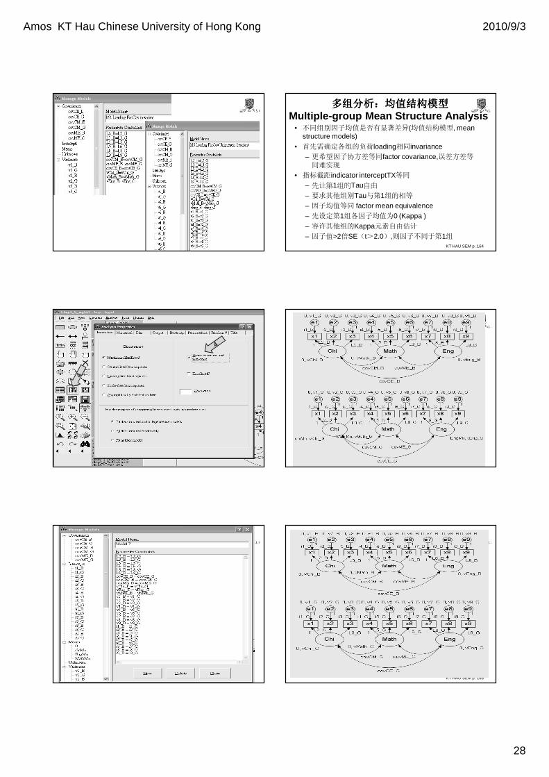
多组分析多组分析多组分析多组分析：：：：均值结构模型均值结构模型均值结构模型均值结构模型Multiple-group Mean Structure Analysis

• 不同组别因子均值是否有显著差异(均值结构模型, mean structure models)

• 首先需确定各组的负荷loading相同invariance– 更希望因子协方差等同factor covariance,误差方差等同难实现

• 指标截距indicator interceptTX等同

– 先让第1组的Tau自由

– 要求其他组别Tau与第1组的相等

– 因子均值等同 factor mean equivalence– 先设定第1组各因子均值为0 (Kappa )– 容许其他组的Kappa元素自由估计

– 因子值>2倍SE（t＞2.0）,则因子不同于第1组




29

KT HAU SEM p. 169

• 结果显示:

– 第2组(女)的KA元素（即语文、数学、英语均值mean）为0.019, -0.102和0.083

– 对应的SE为0.054, 0.041, 0.036

– t-值为0.352、-2.470、2.331

– 这表示:

• 语文自信 -- 男(均值为0)女(均值为0.019)无差异 (t=0.352, n.s.)

• 男生（均值为0）的数学自信高于女生（均值＝ -0.102, t = 2.470）

• 女生的英语自信（均值＝ 0.083）则高于男生（均值为0, t = 2.331）

KT HAU SEM p. 170

多组比较的次序在SEM内,比较多组的因子均值, 一般依下述次序，遂项加上条件:

• 各组因子与指标的从属关系(形态)相同

• 各组因子负荷(loading)相同

• 各组因子间相关(协方差) (variance/covariance)相同

• 各组指标误差(特性)方差(uniqueness)相同

• 各组指标截距(Tau)相同

• 各组因子均值相同(Kappa)

KT HAU SEM p. 171

多组比较检查多组比较检查多组比较检查多组比较检查原則原則原則原則

• 在检查等同条件时,未加等同条件,模型较复杂(df较小)

• 加了等同条件,模型较简单parsimonious (df较大)

• 未加”等同”条件, χ2较小(拟合较好)• 加”等同”条件, χ2较大(拟合较差)• 加”等同”条件,若模型简化甚多,但拟合优只是轻微恶化,则”等同”成立及合理

• 加”等同”条件,若模型简化不多,但拟合优严重恶化,则各组并不等同(等同不成立)

KT HAU SEM p. 172

等同检查等同检查等同检查等同检查第一组第一组第一组第一组其它组别其它组别其它组别其它组别检查检查检查检查(每组解答洽当每组解答洽当每组解答洽当每组解答洽当proper 外外外外…)

型态等同依先验(a priori)模型,估计各参数(parameter)

依先验模型,估计各自由参数

每组拟合优良good fit

Load等同估计各自由Loading

Loading invariant 拟合优fit无严重恶化

var/covar等同

估计各自由var/covar

var/covar invariant

拟合优fit无严重恶化

uniqueness等同

估计各自由uniqueness

uniqueness invariant


intercept 等同

自由估计intercept intercept invariant


Factor mean 等同

fixed at zero freely estimated 每组mean与第一组(或他组)无显著差异significant difference

多组比较设定方法多组比较设定方法多组比较设定方法多组比较设定方法

KT HAU SEM p. 173


X 专题专题专题专题: 结构方程建模和结构方程建模和结构方程建模和结构方程建模和

分析步骤分析步骤分析步骤分析步骤X Issues: Model

Specification and analyses侯傑泰(侯杰泰侯杰泰侯杰泰侯杰泰)

Kit-Tai Hau香港中文大学教育心理系香港中文大学教育心理系香港中文大学教育心理系香港中文大学教育心理系

Educational Psychology Dept, The Chinese University of Hong Kong

使用时请着明出处使用时请着明出处使用时请着明出处使用时请着明出处KT HAU SEM p. 174

专题专题专题专题: 结构方程建模和分析步骤结构方程建模和分析步骤结构方程建模和分析步骤结构方程建模和分析步骤Model Specification and analyses

A. 验证模型与产生模型Confirmatory, Model generation

• 纯粹验证（strictly confirmatory，SC）

• 心目中只有一个模型

• 这类分析不多，无论接受还是拒绝，仍希望有更佳的选择

• 选择模型（alternative models，AM）

• 从拟合的优劣，决定那个模型最为可取

• 但我们仍常做一些轻微修改，成为MG类的分析


30

KT HAU SEM p. 175

• 产生模型（model generating，MG)

• 先提出一个或多个基本模型

• 基于理论或数据，找出模型中拟合欠佳的部份

• 修改模型，通过同一或其他样本，检查修正模型model respecification的拟合程度，目的在于产生一个最佳模型

KT HAU SEM p. 176

B. 结构方程分析步骤• 模型建构（model specification）,指定

• 观测变量与潜变量（因子）的关系

• 各潜变量间的相互关系（指定哪些因子间有相关或直接效应direct effect）

• 在复杂的模型中，可以限制constrain因子负荷loading或因子相关系数等参数的数值或关系（例如，2个因子间相关系数correlation等于0.3；2个因子负荷必须相等）

• 模型拟合(model fitting)• 通常用 ML作模型参数的估计(versus 回归分

析，通常用所最小二乘方法拟合模型，相应的参数估计称为最小二乘估计 )

KT HAU SEM p. 177

C. 模型评价（model assessment）

– 结构方程的解solution是否适当proper，估计是否

收敛，各参数估计值是否在合理范围内（例如，相关系数在 +1与－1之内）

χ2

KT HAU SEM p. 178

– 参数与预设模型的关系是否合理。当然数据分析可能出现一些预期以外的结果，但各参数绝不应出现一些互相矛盾，与先验假设有严重冲突的现象

– 检视多个不同类型的整体拟合指数，如NNFI/TLI、CFI、RMSEA 和χ2等

– 含较多因子的复杂模型中，无论是否删去某一两个路径（固定它们为0），对整个模型拟合影响不大

– 应当先检查每一个测量模型 measurement model

KT HAU SEM p. 179

• D.模型修正模型修正模型修正模型修正（（（（model modification ））））– 依据理论或有关假设，提出一个或数个合理的先验模型a priori model

– 检查潜变量（因子）与指标（题目）间的关系，建立测量模型measurement model

– 可能增删或重组题目– 若用同一样本数据去修正重组测量模型，再检查新模型的拟合指数，这十分接近探索性因素分析（exploratory factor analysis，EFA），所得拟合指数，不足以说明数据支持或验证模型

– 可以循序渐进地，每次只检查含2个因子的模型，确立测量模型部分的合理后，最后才将所有因子合并成预设的先验模型，作一个总体检查

– 对每一模型，检查标准误、t值、标准化残差std residuals、修正指数Modification index MI、参数期望改变值expected change、及各种拟合指数fit index，据此修改模型并重复步骤。

– 这最后的模型是依据某一个样本数据修改而成，最好用另一个独立样本，交互确定cross-validate

KT HAU SEM p. 180

参数估计和拟合函数参数估计和拟合函数参数估计和拟合函数参数估计和拟合函数

Parameter Estimation and Fit Function• 目标是找一些参数parameter使得再生/隐含implied/

reproduced 协方差矩阵与样本协方差矩阵“差距”最小

• 拟合透過拟合函数fit function• 多种拟合函数，参数估计值可能不同

– 工具变量 (IV, instrumental variable)；– 两阶段最小二乘 ( TSLS, two-stage least squares)；– 无加权最小二乘 (ULS, unweighted least squares)；– 最大似然 (ML, maximum likelihood)；– 广义最小二乘 (GLS, generalized least squares)；– 一般加权最小二乘 (WLS, generally weighted least sq)– 对角加权最小二乘 (DWLS, diagonally weighted least sq)

)(θΣ S


31

KT HAU SEM p. 181


XI 专题专题专题专题: 涉及数据的问题涉及数据的问题涉及数据的问题涉及数据的问题XI Issues on data




KT HAU SEM p. 182

专题专题专题专题: 涉及数据的问题涉及数据的问题涉及数据的问题涉及数据的问题

issues on data• 样本容量Sample Size

– 样本:愈大愈好

– 每个因子上多设计几题，预试协助删去一些不好的题目

– 最后每个因子应有3个或更多的题目

• 数据类型Data Type– 绝大部份分析基于皮尔逊（Pearson）相关(假設等比/等距数据interval/ratio data)

– 来自等级（顺序）量表（ordinal scale），改用多项（polyserial）相关系数，并与渐近方差矩阵(asymptotical covariance matrix，ACM)合用，以WLS法拟合模型，除非N很大，额外需要的ACM矩阵多不稳定

KT HAU SEM p. 183

• 可否应用相关矩阵作分析？– SEM建立在方差和协方差分析上– 用相关矩阵，大多数情况下正确– 在某些况下并不正确(见Cudeck, 1989 ):

• 限制因子方差为 1，同时限制某指标的因子负荷不等于零

• 同一个因子，限制其两个或以上指标的因子负荷，不等于零

• 同一个因子的两个或以上指标，限制其因子负荷相同

• 不同因子的两个或以上指标，限制其因子负荷相同

• 限制两个或以上内生潜变量的误差相等

KT HAU SEM p. 184

专题专题专题专题:涉及模型拟合涉及模型拟合涉及模型拟合涉及模型拟合fitting 的问题的问题的问题的问题

• 忽略测量误差measurement error所引致的错误

– 方差（变异量）variance

• x变异量var＝变异量＋误差变异量

• 除非 var 等于零，传统统计高估了变量的真正变异量

– 相关correlation和回归参数regression coefficient

ξ δδ

))var()var((* xξγγ =

71.0)7.0(5.0 212 ==ξηr

( ) 21yyxxxy rrrr =ξη

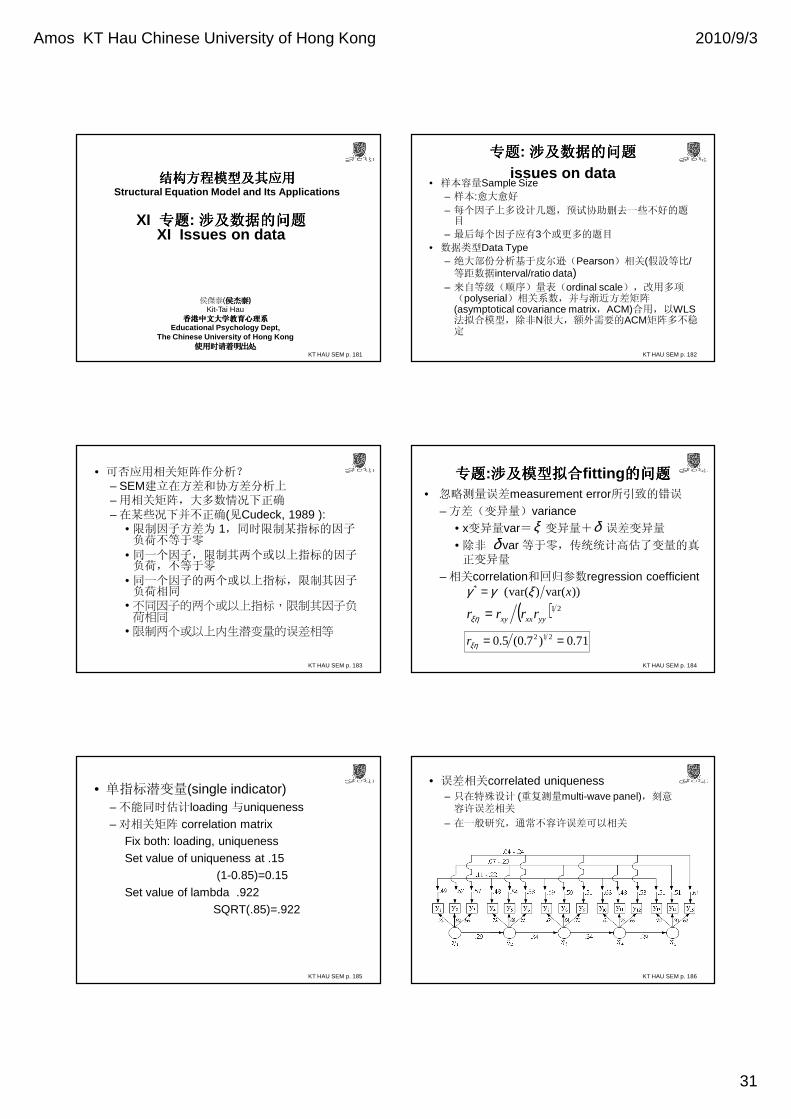
KT HAU SEM p. 185

• 单指标潜变量(single indicator)– 不能同时估计loading 与uniqueness

– 对相关矩阵 correlation matrixFix both: loading, uniqueness

Set value of uniqueness at .15

(1-0.85)=0.15

Set value of lambda .922

SQRT(.85)=.922

KT HAU SEM p. 186

• 误差相关correlated uniqueness– 只在特殊设计 (重复测量multi-wave panel)，刻意容许误差相关

– 在一般研究，通常不容许误差可以相关


32

KT HAU SEM p. 187

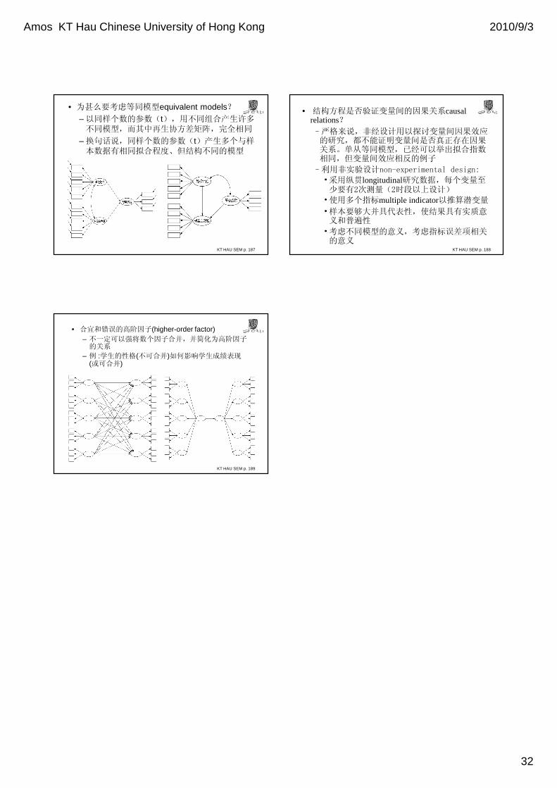
• 为甚么要考虑等同模型equivalent models？

– 以同样个数的参数（t），用不同组合产生许多不同模型，而其中再生协方差矩阵，完全相同

– 换句话说，同样个数的参数（t）产生多个与样本数据有相同拟合程度、但结构不同的模型

KT HAU SEM p. 188

• 结构方程是否验证变量间的因果关系causal relations？–严格来说，非经设计用以探讨变量间因果效应的研究，都不能证明变量间是否真正存在因果关系。单从等同模型，已经可以举出拟合指数相同，但变量间效应相反的例子

–利用非实验设计non-experimental design:

•采用纵贯longitudinal研究数据，每个变量至少要有2次测量（2时段以上设计）

•使用多个指标multiple indicator以推算潜变量

•样本要够大并具代表性，使结果具有实质意义和普遍性

•考虑不同模型的意义，考虑指标误差项相关的意义

KT HAU SEM p. 189

• 合宜和错误的高阶因子(higher-order factor)– 不一定可以强将数个因子合并，并简化为高阶因子的关系

– 例 :学生的性格(不可合并)如何影响学生成绩表现(或可合并)