Embed Size (px)
Citation preview

CafeMol 0.2.0 manual
Hiroo Kenzaki,
Nobuyasu Koga, Shinji Fujiwara, Naoto Hori, Ryo Kanada,
Kei-ichi Okazaki, Xin-Qiu Yao, and
Shoji Takada
Department of Biophysics, Kyoto University
August 10, 2009c©Kyoto University

ii
Contents
0.1 Contributors . . . . . . . . . . . . . . . . . . . . . . . . . . . vii
0.2 License . . . . . . . . . . . . . . . . . . . . . . . . . . . . . . . vii
0.3 Bug reports . . . . . . . . . . . . . . . . . . . . . . . . . . . . viii
0.4 Acknowledgement . . . . . . . . . . . . . . . . . . . . . . . . . viii
1 Introduction 1
1.1 Concept of coarse-grained MD . . . . . . . . . . . . . . . . . 1
1.2 Simulating proteins at work . . . . . . . . . . . . . . . . . . . 4
2 Getting started 5
2.1 About the code . . . . . . . . . . . . . . . . . . . . . . . . . . 5
2.2 How to install CafeMol . . . . . . . . . . . . . . . . . . . . . . 5
2.3 How to execute CafeMol . . . . . . . . . . . . . . . . . . . . . 6
2.4 Size limit and memory resource . . . . . . . . . . . . . . . . . 7
3 Simulation methods 9
3.1 Units in CafeMol . . . . . . . . . . . . . . . . . . . . . . . . . 9
3.2 Model and energy function . . . . . . . . . . . . . . . . . . . 9
3.2.1 Off-lattice Go model for proteins . . . . . . . . . . . . 9
3.2.2 Multiple-basin model for proteins . . . . . . . . . . . . 12
3.2.3 Elastic network model of proteins . . . . . . . . . . . . 15
3.2.4 DNA model . . . . . . . . . . . . . . . . . . . . . . . . 15
3.2.5 Lipid model . . . . . . . . . . . . . . . . . . . . . . . . 15
3.2.6 Interaction between molecules . . . . . . . . . . . . . . 15
3.3 Molecular move algorithm . . . . . . . . . . . . . . . . . . . . 15
3.3.1 Constant temperature “Newtonian” dynamics . . . . . 15
3.3.2 Langevin MD . . . . . . . . . . . . . . . . . . . . . . . 16
3.3.3 Simple minimization (not implemented) . . . . . . . . 18
3.4 Simulation protocol . . . . . . . . . . . . . . . . . . . . . . . . 18
3.4.1 Constant temperature MD . . . . . . . . . . . . . . . 18
3.4.2 Searching TF . . . . . . . . . . . . . . . . . . . . . . . 18
3.4.3 Simulated annealing . . . . . . . . . . . . . . . . . . . 19
3.4.4 Minimization (not implemented) . . . . . . . . . . . . 19
3.4.5 Switching Go potential . . . . . . . . . . . . . . . . . . 19
iii
iv CONTENTS
3.4.6 Switching bias in multiple basin potential . . . . . . . 19
4 Files and data format 21
4.1 Input files . . . . . . . . . . . . . . . . . . . . . . . . . . . . . 21
4.1.1 PDB file (.pdb) . . . . . . . . . . . . . . . . . . . . . . 21
4.1.2 Native-info file(.ninfo) . . . . . . . . . . . . . . . . . . 22
4.1.3 Input file (.inp) . . . . . . . . . . . . . . . . . . . . . . 26
4.1.4 Parameter file (.para) . . . . . . . . . . . . . . . . . . 26
4.2 Output files . . . . . . . . . . . . . . . . . . . . . . . . . . . . 28
4.2.1 PDB file (.pdb) . . . . . . . . . . . . . . . . . . . . . . 28
4.2.2 CARD coordinate (.crd) and velocity (.velo) . . . . . 28
4.2.3 DCD coordinate (.dcd) and velocity (.vdcd) . . . . . . 30
4.2.4 Movie file (.movie) . . . . . . . . . . . . . . . . . . . . 31
4.2.5 Data file (.data) . . . . . . . . . . . . . . . . . . . . . 32
4.2.6 Time-series file (.ts) . . . . . . . . . . . . . . . . . . . 32
4.2.7 Native-info file(.ninfo) . . . . . . . . . . . . . . . . . . 34
5 Input file: How to make 35
5.1 General rules of input files . . . . . . . . . . . . . . . . . . . . 35
5.2 <<<< filenames (required) . . . . . . . . . . . . . . . . . . . 36
5.3 <<<< job cntl (required) . . . . . . . . . . . . . . . . . . . . 38
5.4 <<<< unit and state (required) . . . . . . . . . . . . . . . . 39
5.5 <<<< initial structure (optional) . . . . . . . . . . . . . . . 41
5.6 <<<< initial lipid (not implemented) . . . . . . . . . . . . . 42
5.7 <<<< energy function (required) . . . . . . . . . . . . . . . 42
5.8 <<<< md information (required) . . . . . . . . . . . . . . . 45
5.9 <<<< sequence (optional) . . . . . . . . . . . . . . . . . . . 48
5.10 <<<< searching tf (optional) . . . . . . . . . . . . . . . . . . 48
5.11 <<<< annealing (optional) . . . . . . . . . . . . . . . . . . . 49
5.12 <<<< multiple go (optional) . . . . . . . . . . . . . . . . . . 49
5.13 <<<< native info simN (N can be 1, 2,,,)(optional) . . . . . 50
5.13.1 All-in-one-file style . . . . . . . . . . . . . . . . . . . . 51
5.13.2 One-by-one-file style . . . . . . . . . . . . . . . . . . . 51
5.14 <<<< redefine para (optional) . . . . . . . . . . . . . . . . . 51
5.15 <<<< energy para (optional) . . . . . . . . . . . . . . . . . . 52
5.16 <<<< neighbor dist (optional) . . . . . . . . . . . . . . . . . 53
5.17 <<<< mass friction (optional)] . . . . . . . . . . . . . . . . . 53
5.18 <<<< del interaction (optional) . . . . . . . . . . . . . . . . 54
5.19 <<<< bridge para (optional) . . . . . . . . . . . . . . . . . . 54
5.20 <<<< pulling para (optional) . . . . . . . . . . . . . . . . . 55
5.21 <<<< anchor para (optional) . . . . . . . . . . . . . . . . . 55
5.22 <<<< fix para (optional) . . . . . . . . . . . . . . . . . . . . 56
5.23 <<<< elastic network (optional) . . . . . . . . . . . . . . . . 56
5.24 <<<< in box (optional) . . . . . . . . . . . . . . . . . . . . . 56

CONTENTS v
6 Examples: Input and output 59
6.1 Protein native dynamics and (un)folding with Go model atconstant T . . . . . . . . . . . . . . . . . . . . . . . . . . . . 596.1.1 Input & Output . . . . . . . . . . . . . . . . . . . . . 59
6.2 Automatic TF search . . . . . . . . . . . . . . . . . . . . . . . 596.2.1 Input & Output . . . . . . . . . . . . . . . . . . . . . 60
6.3 Conformational transition simulation with multiple basin modelat constant temperature . . . . . . . . . . . . . . . . . . . . . 606.3.1 Input & Output . . . . . . . . . . . . . . . . . . . . . 60
6.4 Cyclic conformational change simulation by switching Go modelat constant temperature . . . . . . . . . . . . . . . . . . . . . 606.4.1 Input & Output . . . . . . . . . . . . . . . . . . . . . 60
6.5 Rotary motion of F1-ATPase by switching Go model at con-stant temperature . . . . . . . . . . . . . . . . . . . . . . . . 616.5.1 Input & Output . . . . . . . . . . . . . . . . . . . . . 61

vi CONTENTS

Preface
CafeMol is a general-purpose coarse-grained (CG) biomolecular modelingand simulation software. It can simulate proteins, nucleic acids, lipid mem-brane and their mixture with various CG models. (At this stage, though,only the protein part is publicly available)
0.1 Contributors
The main contributor of CafeMol is Hiroo Kenzaki. The chief contributorfor the earlier version of CafeMol, called CaFold(Koga and Takada 2001),is Nobuyasu Koga. Other key contributors of CafeMol are (in alphabeticalorder), Shinji Fujiwara, Naoto Hori, Ryo Kanada, Kei-ichi Okazaki, andXin-Qiu Yao. The CafeMol project is directed by Shoji Takada.
Contact address is [email protected].
0.2 License
CafeMol is the non-commercial software that the user can use, modify, andimprove the CafeMol source code at ones own expense. The source code ofCafeMol is available for the internal use only at this moment: The user shallnot distribute or transfer CafeMol, and any modifications, improvements, orderivatives to CafeMol that the user may create.
CafeMol is a research tool still in the development stage, that is beingsupplied “as is,” without any accompanying services or improvements fromdevelopers and the program is distributed to enable users to utilize CafeMolin their researches. Developers accept no obligation to provide maintenancenor does it guarantee expected functionality of CafeMol or of any part ofCafeMol.
Any published work which utilizes CafeMol should include the citationsuch as “The CafeMol project, H. Kenzaki, N. Koga, S. Fujiwara, N. Hori, R.Kanada, K. Okazaki, X. Yao, and S. Takada, url; http://www.cafemol.org”.
vii
viii PREFACE
0.3 Bug reports
CafeMol is an infant program, most likely with many bugs. We are of courseeager to remove them as much as possible. Thus, we strongly ask users to re-port bugs when they find them. Contact address is [email protected].
0.4 Acknowledgement
CafeMol contains a set of IO utility subroutines, UTILKOTO, coded byShigeru Obara. CafeMol development has been supported by Research andDevelopment of the Next-Generation Integrated Simulation of Living Mat-ter, a part of the Development and Use of the Next-Generation Supercom-puter Project of the Ministry of Education, Culture, Sports, Science andTechnology.
Chapter 1
Introduction
CafeMol is a general-purpose coarse-grained (CG) biomolecular modelingand simulation software. It can simulate proteins, nucleic acids, lipid mem-brane, and their mixture with various CG models. (At this stage, though,only the protein part is publicly available)
1.1 Concept of coarse-grained MD
Molecular dynamics (MD) simulation of biomolecules has long been used fora variety of studies in biology at molecular level. Majority of them employall-atom representation with some force fields and classical mechanics asthe principle of dynamics. Albeit their enormous success, all-atom MDsstill have serious limitation in time scale. All-atom MD reaches up to atbest microsecond at the moment, but typical biological phenomena takemilliseconds, seconds, or longer. Thus, most of biologically relevant eventscannot be simulated directly by all-atom MDs, unfortunately. In such asituation, a strategy of coarse-graining the molecular representation has beentaken many occasion. CafeMol is developed on this line. By coarse-graining,we can easily simulate biological events that correspond to much longer timescale. Such a coarse-grained (CG) model is designed often based on someknowledge of all-atom models. Multiscale simulation methods often provideus methods to determine parameters in CG model based on all-atom model.
Coarse graining is not a unique procedure at all. Each CG model isbased on its developer’s perspectives. CafeMol takes quite a characteris-tic approach of coarse-graining, which is based on specific perspectives onbiomolecular system. Here, we briefly describe it.
Proteins have evolved to have ability of folding to their own native struc-tures. Even if a protein is intrinsically disordered as an isolated molecule, itmost often folds upon binding to its partner and thus foldability in this con-text, means the ability to fold upon binding. If we look at native structures
1
2 CHAPTER 1. INTRODUCTION
of proteins in PDB, we notice that, overall, most side-chains are extremelywell-packed in their cores. Whenever you find a charge in the core, it iseither paired with counter charge or functionally essential. Thus, exceptfunctional reason, the interaction at the native is highly consistent, whichwas termed many years ago “consistency principle” by Go(Go 1983). Pro-teins gained, through evolution, the foldability by minimizing the frustrationat their native structures, which is called “principle of the minimum frus-tration” by Wolynes(Bryngelson and Wolynes 1987). The effective energytakes the minimal value at the native, and as the conformation deviatesfrom the native, the energy, on average, increases, which leads to funnel-likepicture of the energy landscape, first invented by Onuchic(Leopold, Mon-tal, and Onuchic 1992). We emphasize that completeness of the side-chainspacking are outstanding, in particular. In this sense, the native state is ofsome similarity to crystal or amorphous. On the other hand, the denaturedstate is characterized with low-level side-chain packing and large fluctuationand thus resembles fluid. Coarse-graining is relatively easy for fluid phasebecause it is essentially statistical ensemble that decides the property ofpolymers. All you need is statistical average over the ensemble, which makescoarse-graining easier. The native state, however, is more difficult to be de-scribed by CG model because it is defined by high level of side-chain packing,a very specific and non-self-averaging property. If the side-chain architectureis lost by coarse-graining, very surely you lose those specific interactions, tosome extent. Thus physics based coarse-graining is not very effective forapproximating the native state. This is the stage we should bring the evo-lutionary perspective. Remember that we know that proteins have evolvedto have the minimal frustration. This principle can be used as a guidingprinciple for coarse-graining. Namely, we assume, as an extreme, that allthe interactions found at the native structure are attractive. Simultane-ously, we require that the protein can take nearly random coil at sufficientlyhigh temperature. These two extreme requirements lead to the so-called Gomodel, first developed in the lattice representation of proteins. However, ofcourse, protein dynamics near the native is not well approximated by thelattice representation. Indeed, protein dynamics near the native structuremay be well-approximated by quasi-harmonic potential, such as elastic net-work model (ENM) of Tirion(Tirion 1996). The ENM model is good onlynear the native and is not appropriate for the denatured state. A modelthat is similar to the ENM near the native structure and simultaneouslythat share the concept of the lattice Go model is required. This led to theidea of off-lattice Go model. Off-lattice Go model represents quasi-harmonicfluctuation near the native structure and simultaneously realize perfect fun-nel energy landscape. So, Go model is often called the perfect-funnel model,the native-centric model, or structure-based model. CafeMol employs off-lattice Go model developed by Clementi, Nyemyer, and Onuchic(Clementi,Nymeyer, and Onuchic 2000), and its derivative, as a basic CG model for
1.1. CONCEPT OF COARSE-GRAINED MD 3
proteins.
In contrast, lipid membrane is fluid-like. It is well-known that lipids candiffuse laterally in lipid membrane, which directly suggest fluidity. Fluctu-ation on vertical direction is also noticeable. Thus, physics-based coarse-graining is expected to work better for lipid membrane. Indeed, transfer-able CG models of membrane have been developed and widely used. It isalso noted that lipids are much shorter polymer than proteins and lipidsthemselves are not explicitly encoded in genome. Thus no direct evolution-ary pressure exists so that lipid take a specific structure. Structure-basedmodel, or Go model is not appropriate. Thus, Go model is not used at allfor lipid membrane in CafeMol.
Nucleic acids are in between proteins and lipids, as for the degree ofevolutionary design. Some RNAs work as ribozyme, for which Go modeldescription is perhaps the best choice because base sequence for these RNAmust have evolved to have the foldability. DNA makes duplex in most situ-ations, and thus Go-like description is useful to support the B-DNA duplexshape. Yet, since nucleic acids always contain a lot of negative charges, elec-trostatic interactions play major roles in every situations, and thus physicalinteraction energy is also of crucial importance. CafeMol employs CG modelof duplex DNA that combine Go-like interaction and physical interactions.
Perhaps, the most difficult decision is about the interaction between dif-ferent biomolecules. Candidates are physical interactions, Go interactions,and both of them. We recommend to classify inter-molecular interactionsinto two types: (sequence-) specific and generic. The specific interaction, bydefinition, is specific to the particular pair of molecules, and thus is sequencedependent. It is also characterized by relatively high affinity. Thus, removalof side-chain architecture in the CG model lose the van der Waals packingand, most likely, destabilizes the specific interaction. Simultaneously, it canbe thought that the specific interaction was designed by the evolutionarypressure. They together legitimate the use of Go interaction for the spe-cific interaction. (There is no problem to add physical interaction, togetherwith Go interaction, to the specific interaction) On the other hand, genericinteraction is often weak and, by definition, does not sensitively depend onthe sequence. Thus, coarse-graining may not destabilize the generic interac-tion very seriously. Thus, we recommend to use physical interaction for thegeneric interactions. For example, interactions between proteins and lipidmembranes are generic. Protein-DNA interactions depend on the cases. Thecomplex of transcription factor and DNA is best modeled by both Go andphysical interactions. Nucleosome may be modeled by physical interactionsbetween histone proteins and duplex DNA.

4 CHAPTER 1. INTRODUCTION
1.2 Simulating proteins at work
Biomolecules, primarily proteins and some RNA’s work as biomolecular ma-chines. To understand the working principles of such machines, moleculardynamics simulations are potentially very powerful because they providetime-dependent structural information. By using CG model, we can simu-late the protein dynamics in a time scale comparable to that the biomolec-ular machines indeed work. Yet, the long-time simulation alone is not suf-ficient to simulate such machines at work, because proteins actively move(work) driven by some external energy source. Often, the energy source isof chemical nature, e.g., chemical reaction, ion passage, and so on. CG MDcannot directly deal with such chemical events. For mimicking these energysource, we proposed to “switch” the energy function in certain ways(Kogaand Takada 2006). By switching, we put some energy into the system. Pro-teins start to “work” as machines.
One of the key advantages of CafeMol, in comparison with other MDpackages, is to equip various means to conduct dynamic “switching” simu-lations, which try to mimic energy source given into the system and switch onthe active motion of the machines. Molecular motors such as F1-ATPase(Kogaand Takada 2006) and kinesin are wonderful examples of these functions.
Chapter 2
Getting started
2.1 About the code
CafeMol is written in FORTRAN90 with MPI and C pre-processing direc-tives. Thus, it can run virtually any computer that has both FORTRAN90and C compiler. In an ordinary way, files having extension ’.F90’ are auto-matically and firstly pre-processed by C compiler.
2.2 How to install CafeMol
The following steps are typically needed.
1. Download CafeMol xxx.tar.gz file, and extract it.
$tar zxvf CafeMol xxx.tar.gz
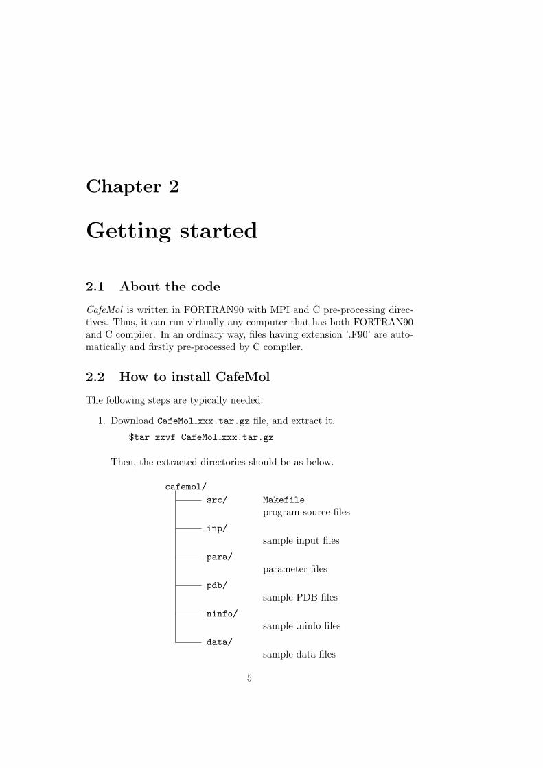
Then, the extracted directories should be as below.
cafemol/
src/ Makefile
program source files
inp/
sample input files
para/
parameter files
pdb/
sample PDB files
ninfo/
sample .ninfo files
data/
sample data files
5
6 CHAPTER 2. GETTING STARTED
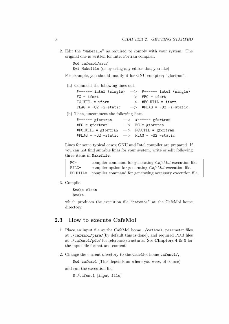
2. Edit the “Makefile” as required to comply with your system. Theoriginal one is written for Intel Fortran compiler.
$cd cafemol/src/
$vi Makefile (or by using any editor that you like)
For example, you should modify it for GNU compiler; “gfortran”,
(a) Comment the following lines out.
#------ intel (single) —> #------ intel (single)
FC = ifort —> #FC = ifort
FC UTIL = ifort —> #FC UTIL = ifort
FLAG = -O2 -i-static —> #FLAG = -O2 -i-static
(b) Then, uncomment the following lines.
#------ gfortran —> #------ gfortran
#FC = gfortran —> FC = gfortran
#FC UTIL = gfortran —> FC UTIL = gfortran
#FLAG = -O2 -static —> FLAG = -O2 -static
Lines for some typical cases; GNU and Intel compiler are prepared. Ifyou can not find suitable lines for your system, write or edit followingthree items in Makefile.
FC= compiler command for generating CafeMol execution file.FALG= compiler option for generating CafeMol execution file.FC UTIL= compiler command for generating accessory execution file.
3. Compile.
$make clean
$make
which produces the execution file “cafemol” at the CafeMol homedirectory.
2.3 How to execute CafeMol
1. Place an input file at the CafeMol home ./cafemol, parameter filesat ./cafemol/para/(by default this is done), and required PDB filesat ./cafemol/pdb/ for reference structures. See Chapters 4 & 5 forthe input file format and contents.
2. Change the current directory to the CafeMol home cafemol/,
$cd cafemol (This depends on where you were, of course)
and run the execution file,
$./cafemol [input file]
2.4. SIZE LIMIT AND MEMORY RESOURCE 7
If you use MPI, command should be
$impijob ./cafemol [input file]
(This is an example in case of Intel MPI.)
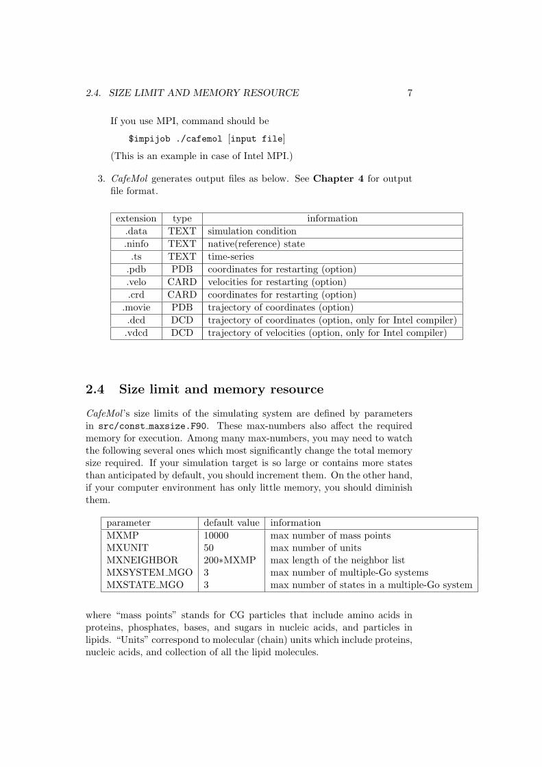
3. CafeMol generates output files as below. See Chapter 4 for outputfile format.
extension type information
.data TEXT simulation condition
.ninfo TEXT native(reference) state
.ts TEXT time-series
.pdb PDB coordinates for restarting (option)
.velo CARD velocities for restarting (option)
.crd CARD coordinates for restarting (option)
.movie PDB trajectory of coordinates (option)
.dcd DCD trajectory of coordinates (option, only for Intel compiler)
.vdcd DCD trajectory of velocities (option, only for Intel compiler)
2.4 Size limit and memory resource
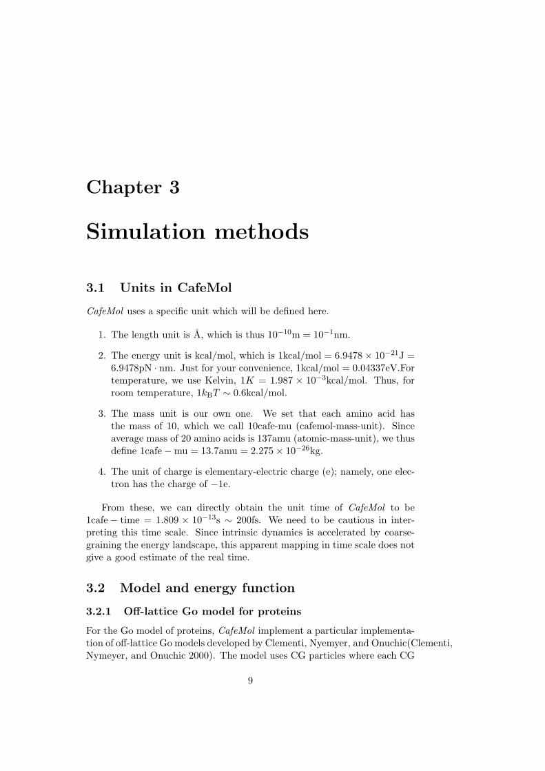
CafeMol ’s size limits of the simulating system are defined by parametersin src/const maxsize.F90. These max-numbers also affect the requiredmemory for execution. Among many max-numbers, you may need to watchthe following several ones which most significantly change the total memorysize required. If your simulation target is so large or contains more statesthan anticipated by default, you should increment them. On the other hand,if your computer environment has only little memory, you should diminishthem.
parameter default value information
MXMP 10000 max number of mass pointsMXUNIT 50 max number of unitsMXNEIGHBOR 200∗MXMP max length of the neighbor listMXSYSTEM MGO 3 max number of multiple-Go systemsMXSTATE MGO 3 max number of states in a multiple-Go system
where “mass points” stands for CG particles that include amino acids inproteins, phosphates, bases, and sugars in nucleic acids, and particles inlipids. “Units” correspond to molecular (chain) units which include proteins,nucleic acids, and collection of all the lipid molecules.

8 CHAPTER 2. GETTING STARTED
Regarding the memory usage, MXMP has the largest impact. In par-ticular, the neighbor list array is probably the largest array used in thecode.
Chapter 3
Simulation methods
3.1 Units in CafeMol
CafeMol uses a specific unit which will be defined here.
1. The length unit is A, which is thus 10−10m = 10−1nm.
2. The energy unit is kcal/mol, which is 1kcal/mol = 6.9478× 10⁻²¹J =6.9478pN · nm. Just for your convenience, 1kcal/mol = 0.04337eV.Fortemperature, we use Kelvin, 1K = 1.987 × 10⁻³kcal/mol. Thus, forroom temperature, 1kBT ∼ 0.6kcal/mol.
3. The mass unit is our own one. We set that each amino acid hasthe mass of 10, which we call 10cafe-mu (cafemol-mass-unit). Sinceaverage mass of 20 amino acids is 137amu (atomic-mass-unit), we thusdefine 1cafe−mu = 13.7amu = 2.275× 10⁻²⁶kg.
4. The unit of charge is elementary-electric charge (e); namely, one elec-tron has the charge of −1e.
From these, we can directly obtain the unit time of CafeMol to be1cafe− time = 1.809 × 10⁻¹³s ∼ 200fs. We need to be cautious in inter-preting this time scale. Since intrinsic dynamics is accelerated by coarse-graining the energy landscape, this apparent mapping in time scale does notgive a good estimate of the real time.
3.2 Model and energy function
3.2.1 Off-lattice Go model for proteins
For the Go model of proteins, CafeMol implement a particular implementa-tion of off-lattice Go models developed by Clementi, Nyemyer, and Onuchic(Clementi,Nymeyer, and Onuchic 2000). The model uses CG particles where each CG
9
10 CHAPTER 3. SIMULATION METHODS
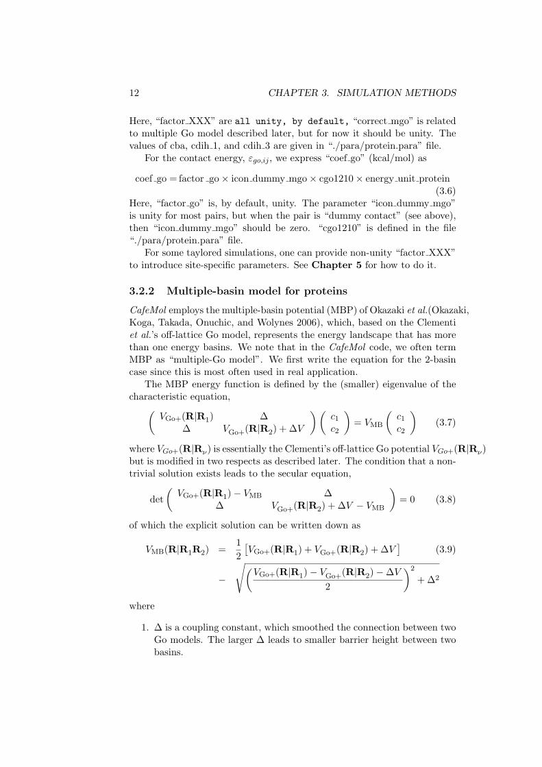
particle represents an amino acid, most often represented as Cα atoms (canbe Cβ , or the center of mass of amino acids, though). For a protein withthe number of amino acids naa , the off-lattice Go model is defined by thepotential energy function,
VGo(R|R0) =∑
ibd
Kb,ibd(bibd − bibd,0)2 +
∑
iba
Kθ,iba(θiba − θiba,0)2 (3.1)
+∑
idih
{
K(1)φ,idih[1− cos(φidih − φidih,0)] + K
(3)φ,idih[1− cos 3(φidih − φidih,0)]
}
+nat contact∑
i<j−3
εgo,ij
[
5
(
rij0
rij
)12
− 6
(
rij0
rij
)10]
+non−native∑
i<j−3
εev
(
d
rij
)12
where
1. R: Cartesian coordinates of the simulated protein as 3naa-dimensionalvector
2. bibd: ibd-th virtual bond length defined as |ribd+1−ribd| of the simulatedprotein, where ri stands for the Cartesian coordinate of the i-th aminoacid (=CG particle).(1 ≤ ibd ≤ naa − 1)
3. θiba: iba-th bond angle between two consecutive virtual bond vectors,riba − riba+1, and riba+2 − riba+1 of the simulated proteins (1 ≤ iba ≤naa − 2)
4. φidih: idih-th dihedral angle around the idih + 1-th virtual bondridih+2 − ridih+1 of the simulated protein. (1 ≤ idih ≤ naa − 3)
5. rij : Distance between i-th and j-th amino acids of the simulated pro-teins.
6. R0: Cartesian coordinates of the native (sometime called reference orfiducial) structure as 3naa-dimensional vector, which corresponds tothe bottom of the folding funnel.
7. All other parameters that have the subscript 0 are the constants whichhave the values of the corresponding variables at the native structureR0.
8. Kb,ibd, Kθ,iba, K(1)φ,idih, K
(3)φ,idih, εgo,ij , εev, and d are the parameters. For
the former 5 parameters, Clementi et al.’s original model uses homoge-neous setting, i.e., the same values for the entire systems. In CafeMol,however, one can uses site-specific parameters, i.e., the parameter val-ues that depend on residues, upon request.

3.2. MODEL AND ENERGY FUNCTION 11
9.nat contact∑
i<j−3: Summation over “native contact pairs”, which are pairs of
amino acids that are physically close to each other at the native (orthe reference) structure. If one of the non-hydrogen atoms in the i-thamino acid is within a threshold distance (inside CafeMol, defined bydfcontact) from one of non-hydrogen atoms in the j-th amino acid, wedefine the pair of the i-th and the j-th amino acids as being nativecontact. Only non-local pairs defined by i < j − 3 are taken intoaccount.
Here, we emphasize that, even though CafeMol uses one bead (mostoften located at Cα atom) per amino acid as the dynamic variablein MD simulations, the native contacts are defined by using ALL-ATOM INFORMATION of the native (reference) structure. Thus,the pdb structure given for the native structure must contain all-atomcoordinates.
10.non−native∑
i<j−3: Summation over pairs that are not in the native contact
pair set. Only non-local pairs defined by i < j − 3 are taken intoaccount.
Inside CafeMol , the parameter values of Kb,ibd, Kθ,iba, K(1)φ,idih, K
(3)φ,idih,
εgo,ij are expressed as the products of several factors.
For example, Kb,ibd, which has the internal name “coef bd” (kcal/mol/A2)is expressed as
coef bd = factor bd× correct mgo× cbd× energy unit protein (3.2)
where “factor bd” and “correct mgo” are unity, by default, and the valueof “cbd” is indicated in “./para/protein.para” file, and one can change it inthe input file, as is described in Chapter 5. The “energy unit protein” isa scaling factor that (approximately) connects energy scale of the proteinmodel to kcal/mol unit. These data will be output in the native-info file(See Chapter 4).
The form is essentially the same for all the local terms. Kθ,iba, K(1)φ,idih,
K(3)φ,idih respectively, are termed “coef ba”, “coef dih1”, and “coef dih2”,
which are given as
coef ba = factor ba× correct mgo× cba× energy unit protein (3.3)
coef dih1 = factor dih× correct mgo× cdih 1× energy unit protein (3.4)
coef dih3 = factor dih× correct mgo× cdih 3× energy unit protein (3.5)
12 CHAPTER 3. SIMULATION METHODS
Here, “factor XXX” are all unity, by default, “correct mgo” is relatedto multiple Go model described later, but for now it should be unity. Thevalues of cba, cdih 1, and cdih 3 are given in “./para/protein.para” file.
For the contact energy, εgo,ij , we express “coef go” (kcal/mol) as
coef go = factor go× icon dummy mgo× cgo1210× energy unit protein(3.6)
Here, “factor go” is, by default, unity. The parameter “icon dummy mgo”is unity for most pairs, but when the pair is “dummy contact” (see above),then “icon dummy mgo” should be zero. “cgo1210” is defined in the file“./para/protein.para” file.
For some taylored simulations, one can provide non-unity “factor XXX”to introduce site-specific parameters. See Chapter 5 for how to do it.
3.2.2 Multiple-basin model for proteins
CafeMol employs the multiple-basin potential (MBP) of Okazaki et al.(Okazaki,Koga, Takada, Onuchic, and Wolynes 2006), which, based on the Clementiet al.’s off-lattice Go model, represents the energy landscape that has morethan one energy basins. We note that in the CafeMol code, we often termMBP as “multiple-Go model”. We first write the equation for the 2-basincase since this is most often used in real application.
The MBP energy function is defined by the (smaller) eigenvalue of thecharacteristic equation,
(
VGo+(R|R1) ∆∆ VGo+(R|R2) + ∆V
)(
c1
c2
)
= VMB
(
c1
c2
)
(3.7)
where VGo+(R|Rν) is essentially the Clementi’s off-lattice Go potential VGo+(R|Rν)but is modified in two respects as described later. The condition that a non-trivial solution exists leads to the secular equation,
det
(
VGo+(R|R1)− VMB ∆∆ VGo+(R|R2) + ∆V − VMB
)
= 0 (3.8)
of which the explicit solution can be written down as
VMB(R|R1R2) =1
2
[
VGo+(R|R1) + VGo+(R|R2) + ∆V]
(3.9)
−
√
(
VGo+(R|R1)− VGo+(R|R2)−∆V
2
)2
+ ∆2
where
1. ∆ is a coupling constant, which smoothed the connection between twoGo models. The larger ∆ leads to smaller barrier height between twobasins.

3.2. MODEL AND ENERGY FUNCTION 13
2. ∆V is to modulate the relative energies of the two basins.
As a reaction coordinate,
χ = ln
(
c2
c1
)
(3.10)
is a convenient quantity. It is negative when the system is in the state 1 andis positive when the system is in the state 2.
Now, VGo+(R|Rν) is to be defined. As was noted, this is conceptuallyjust VGo(R|Rν) of Clementi et al. Purely by technical reasons, we need tointroduce two modifications. We write the VGo+(R|Rν) in the sum of threeterms,
VGo+(R|Rν) = Vlocal(R|Rν) + Vnative-attr(R|Rν) + Vrepul(R|Rν) (3.11)
where the first term is
Vlocal(R|Rν) =∑
ibd
Kb,ibd(bibd − bibd,ν)2 +
∑
iba
Kθ,iba(θiba − θiba,ν)2
+∑
idih
{
K(1)φ,idih[1− cos(φidih − φidih,ν)] (3.12)
+ K(3)φ,idih[1− cos 3(φidih − φidih,ν)]
}
This local potential is slightly different from that of VGo(R|Rν): Namely,three of the K’s are now dependent on i in the following ways;
Kbi = Kb ×min
[
1,ǫb,max
Kb(bi,1 − bi,2)2
]
(3.13)
Kθi = Kθ ×min
[
1,ǫθ,max
Kθ(θi,1 − θi,2)2
]
(3.14)
K(1)φi = K
(1)φ ×min
1,ǫφ,max
K(1)φ [1− cos(φi,1 − φi,2)] + K
(3)φ [1− cos 3(φi,1 − φi,2)]
(3.15)
K(3)φi = K
(3)φ ×min
1,ǫφ,max
K(1)φ [1− cos(φi,1 − φi,2)] + K
(3)φ [1− cos 3(φi,1 − φi,2)]
(3.16)This is introduced so that spring constants should be weakened where
large change is observed between two reference structures. ǫb,max, ǫθ,max and
14 CHAPTER 3. SIMULATION METHODS
ǫφ,max are the cutoffs that define the “large change”. We note that becauseof this, Vlocal(R|{Rν}) is not just a function of the reference structure Rν ,but also depends on other reference structures.
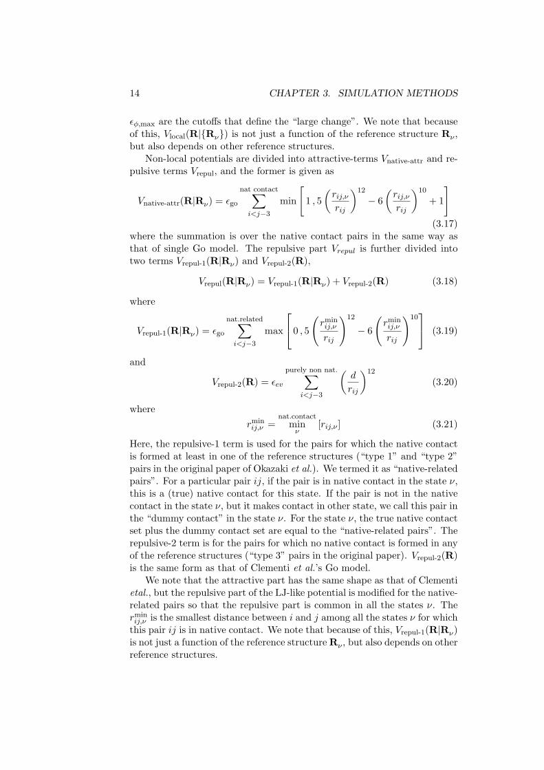
Non-local potentials are divided into attractive-terms Vnative-attr and re-pulsive terms Vrepul, and the former is given as
Vnative-attr(R|Rν) = ǫgo
nat contact∑
i<j−3
min
[
1 , 5
(
rij,ν
rij
)12
− 6
(
rij,ν
rij
)10
+ 1
]
(3.17)where the summation is over the native contact pairs in the same way asthat of single Go model. The repulsive part Vrepul is further divided intotwo terms Vrepul-1(R|Rν) and Vrepul-2(R),
Vrepul(R|Rν) = Vrepul-1(R|Rν) + Vrepul-2(R) (3.18)
where
Vrepul-1(R|Rν) = ǫgo
nat.related∑
i<j−3
max
0 , 5
(
rminij,ν
rij
)12
− 6
(
rminij,ν
rij
)10
(3.19)
and
Vrepul-2(R) = ǫev
purely non nat.∑
i<j−3
(
d
rij
)12
(3.20)
where
rminij,ν =
nat.contactmin
ν[rij,ν ] (3.21)
Here, the repulsive-1 term is used for the pairs for which the native contactis formed at least in one of the reference structures (“type 1” and “type 2”pairs in the original paper of Okazaki et al.). We termed it as “native-relatedpairs”. For a particular pair ij, if the pair is in native contact in the state ν,this is a (true) native contact for this state. If the pair is not in the nativecontact in the state ν, but it makes contact in other state, we call this pair inthe “dummy contact” in the state ν. For the state ν, the true native contactset plus the dummy contact set are equal to the “native-related pairs”. Therepulsive-2 term is for the pairs for which no native contact is formed in anyof the reference structures (“type 3” pairs in the original paper). Vrepul-2(R)is the same form as that of Clementi et al.’s Go model.
We note that the attractive part has the same shape as that of Clementietal., but the repulsive part of the LJ-like potential is modified for the native-related pairs so that the repulsive part is common in all the states ν. Therminij,ν is the smallest distance between i and j among all the states ν for which
this pair ij is in native contact. We note that because of this, Vrepul-1(R|Rν)is not just a function of the reference structure Rν , but also depends on otherreference structures.
3.3. MOLECULAR MOVE ALGORITHM 15
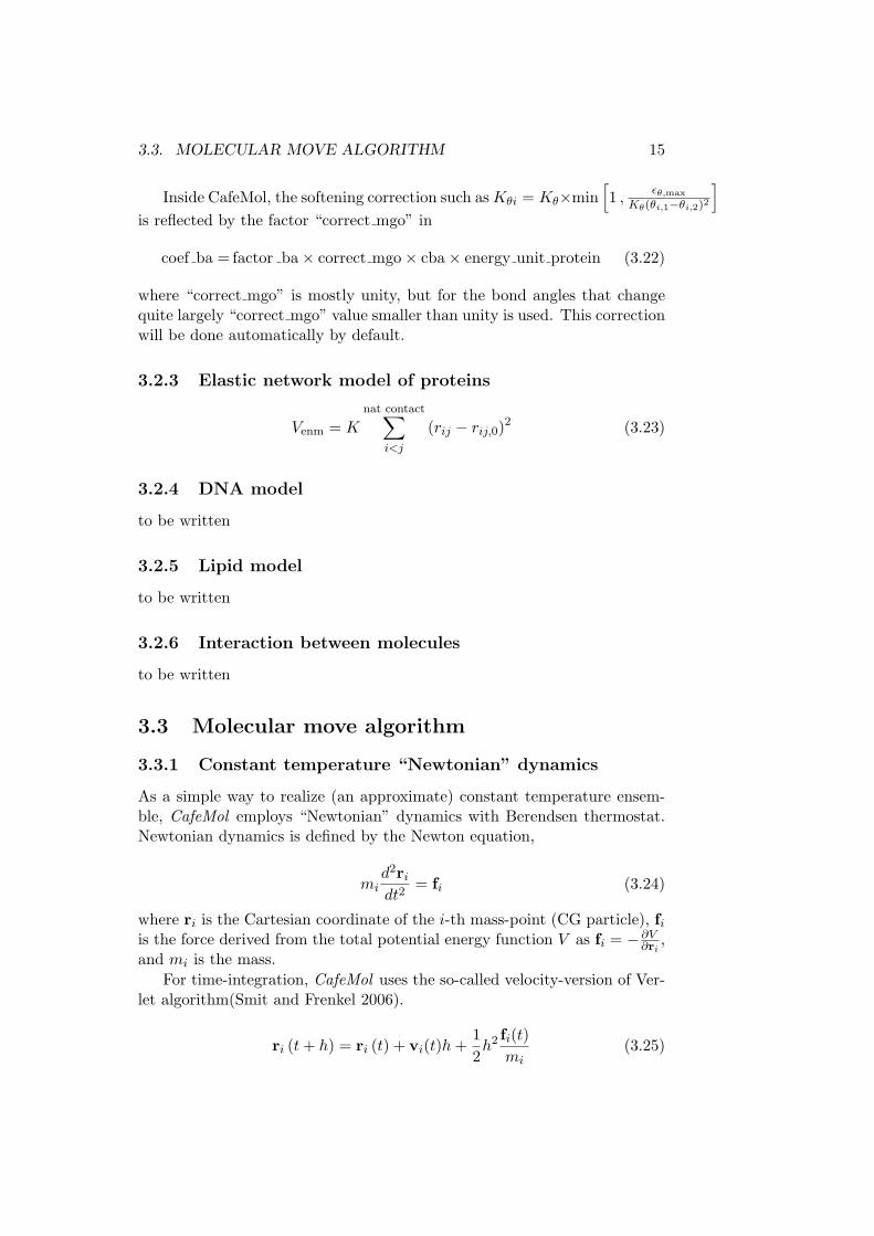
Inside CafeMol, the softening correction such as Kθi = Kθ×min[
1 ,ǫθ,max
Kθ(θi,1−θi,2)2
]
is reflected by the factor “correct mgo” in
coef ba = factor ba× correct mgo× cba× energy unit protein (3.22)
where “correct mgo” is mostly unity, but for the bond angles that changequite largely “correct mgo” value smaller than unity is used. This correctionwill be done automatically by default.
3.2.3 Elastic network model of proteins
Venm = Knat contact∑
i<j
(rij − rij,0)2 (3.23)
3.2.4 DNA model
to be written
3.2.5 Lipid model
to be written
3.2.6 Interaction between molecules
to be written
3.3 Molecular move algorithm
3.3.1 Constant temperature “Newtonian” dynamics
As a simple way to realize (an approximate) constant temperature ensem-ble, CafeMol employs “Newtonian” dynamics with Berendsen thermostat.Newtonian dynamics is defined by the Newton equation,
mid2ri
dt2= fi (3.24)
where ri is the Cartesian coordinate of the i-th mass-point (CG particle), fiis the force derived from the total potential energy function V as fi = − ∂V
∂ri,
and mi is the mass.
For time-integration, CafeMol uses the so-called velocity-version of Ver-let algorithm(Smit and Frenkel 2006).
ri (t + h) = ri (t) + vi(t)h +1
2h2 fi(t)
mi(3.25)
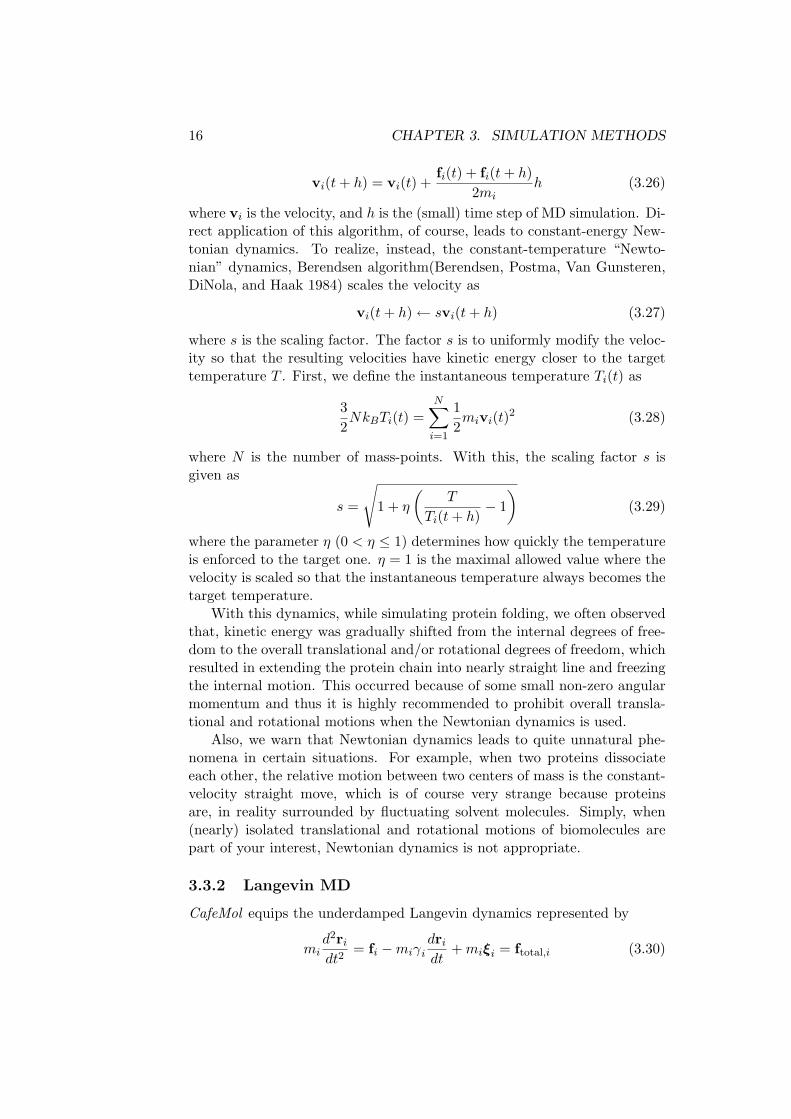
16 CHAPTER 3. SIMULATION METHODS
vi(t + h) = vi(t) +fi(t) + fi(t + h)
2mih (3.26)
where vi is the velocity, and h is the (small) time step of MD simulation. Di-rect application of this algorithm, of course, leads to constant-energy New-tonian dynamics. To realize, instead, the constant-temperature “Newto-nian” dynamics, Berendsen algorithm(Berendsen, Postma, Van Gunsteren,DiNola, and Haak 1984) scales the velocity as
vi(t + h)← svi(t + h) (3.27)
where s is the scaling factor. The factor s is to uniformly modify the veloc-ity so that the resulting velocities have kinetic energy closer to the targettemperature T . First, we define the instantaneous temperature Ti(t) as
3
2NkBTi(t) =
N∑
i=1
1
2mivi(t)
2 (3.28)
where N is the number of mass-points. With this, the scaling factor s isgiven as
s =
√
1 + η
(
T
Ti(t + h)− 1
)
(3.29)
where the parameter η (0 < η ≤ 1) determines how quickly the temperatureis enforced to the target one. η = 1 is the maximal allowed value where thevelocity is scaled so that the instantaneous temperature always becomes thetarget temperature.
With this dynamics, while simulating protein folding, we often observedthat, kinetic energy was gradually shifted from the internal degrees of free-dom to the overall translational and/or rotational degrees of freedom, whichresulted in extending the protein chain into nearly straight line and freezingthe internal motion. This occurred because of some small non-zero angularmomentum and thus it is highly recommended to prohibit overall transla-tional and rotational motions when the Newtonian dynamics is used.
Also, we warn that Newtonian dynamics leads to quite unnatural phe-nomena in certain situations. For example, when two proteins dissociateeach other, the relative motion between two centers of mass is the constant-velocity straight move, which is of course very strange because proteinsare, in reality surrounded by fluctuating solvent molecules. Simply, when(nearly) isolated translational and rotational motions of biomolecules arepart of your interest, Newtonian dynamics is not appropriate.
3.3.2 Langevin MD
CafeMol equips the underdamped Langevin dynamics represented by
mid2ri
dt2= fi −miγi
dri
dt+ miξi = ftotal,i (3.30)

3.3. MOLECULAR MOVE ALGORITHM 17
where mi is the mass, fi is the force derived from the total potential energyfunction V as fi = − ∂V
∂ri, γi is the friction coefficient, and ξi is the random
force (divided by the mass) The latter is a white and Gaussian random forcewith the mean 〈ξi(t)〉 = 0 and the variance 〈ξi(t)ξi(t
′)〉 = 2m−1i γikBTδ(t−
t′)1, where the bracket means the canonical ensemble average, and 1 is a3×3 unit matrix.
For time integration, CafeMol uses a simple algorithm developed byHoneycutt-Thirumalai(Honeycutt and Thirumalai 1992) (or Guo-Thirumalai(Guoand Thirumalai 1995)). Based on the velocity version of the Verlet algo-rithm, this formula is derived by the Taylor expansion about γh and thus isvalid for small γh case. The coordinate update in Verlet formula is
ri (t + h) = ri (t) + vi(t)h +1
2h2 ftotal,i(t)
mi(3.31)
Replacing ftotal,i(t) with its three components, we get,
ri (t + h) = ri (t) + vi(t)h
(
1−γih
2
)
(3.32)
+1
2h2
(
fi(t)
mi+ ξi(t)
)
This is the formula for the coordinate updates in CafeMol. For velocityupdate, the original Verlet formula gives
vi(t + h) = vi(t) +ftotal,i(t) + ftotal,i(t + h)
2mih (3.33)
where ftotal,i(t + h) depends on the velocity at t + h, and thus the formulaneed to be solved self-consistently. We can only derive the closed formulafor small γh limit. Namely, we can get
vi(t + h)
(
1 +γih
2
)
= vi(t)
(
1−γih
2
)
(3.34)
+h
2
(
fi(t)
mi−
fi(t + h)
mi+ ξi(t) + ξi(t + h)
)
Using the approximation
(
1 +γih
2
)
−1
= 1−γih
2+
(
γih
2
)2
+ ... (3.35)
we end up with the formula,
vi(t + h) = vi(t)
(
1−γih
2
)
[
1−γih
2+
(
γih
2
)2]
(3.36)
+h
2
(
1−γih
2
)(
fi(t)
mi−
fi(t + h)
mi+ ξi(t) + ξi(t + h)
)

18 CHAPTER 3. SIMULATION METHODS
where we note that the first line contains a third order term, which can beomitted, but is harmless too. CafeMol exactly uses the above formula forthe velocity update. The random force ξi(t) in finite time step is drawnfrom the Gaussian (normal) distribution with its mean
〈ξi(t)〉 = 0 (3.37)
and its variance⟨
ξi(t)ξi(t′)⟩
=2γikBT
mi
δt,t′
h1 (3.38)
The Langevin dynamics has no problems that we raised in the sectionon constant-temperature Newtonian dynamics. There are some drawbacksin Langevin dynamics, too. First, while simulating protein folding, we ob-served that folding is less cooperative near the transition state and thus isless efficient. For some proteins, we could simulate reversible folding onlywith Newtonian dynamics, but not with Langevin dynamics. Another lim-itation of Langevin dynamics, though perhaps related to the first one, isits ignorance of hydrodynamics interaction. Usually, ignorance of hydrody-namic interaction slows down translational and rotational motion of macro-molecules represented as collection of many small particles. Yet, for generaluse in simulations of biomolecular complex, Langevin dynamics is the firstchoice in CafeMol, at the moment.
3.3.3 Simple minimization (not implemented)
to be written
3.4 Simulation protocol
3.4.1 Constant temperature MD
The constant temperature MD is the most standard simulation protocol inCafeMol. Currently, one can use either constant-temperature “Newtonian”dynamics or Langevin dynamics.
3.4.2 Searching TF
CafeMol uses a bisection method to automatically compute the folding tran-sition temperature TF . Namely, you first specify, in the input file, the lowerand upper bounds of TF . CafeMol first simulates the protein at the mid-point temperature of the upper and lower bounds and see if the protein isnear native conformation for more than half of the simulated time. If yes,this temperature is set as the new lower bound of TF . Otherwise, the simu-lated temperature was set as the new upper bound of TF . With the new setof the lower and the upper bounds, CafeMol repeats the simulation. This
3.4. SIMULATION PROTOCOL 19
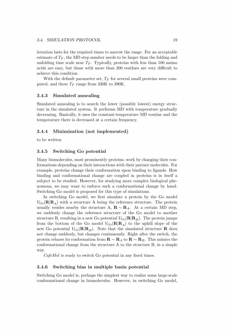
iteration lasts for the required times to narrow the range. For an acceptableestimate of TF , the MD step number needs to be larger than the folding andunfolding time scale near TF . Typically, proteins with less than 100 aminoacids are easy, but those with more than 200 residues are very difficult toachieve this condition.
With the default parameter set, TF for several small proteins were com-puted, and these TF range from 330K to 390K.
3.4.3 Simulated annealing
Simulated annealing is to search the lower (possibly lowest) energy struc-ture in the simulated system. It performs MD with temperature graduallydecreasing. Basically, it uses the constant-temperature MD routine and thetemperature there is decreased at a certain frequency.
3.4.4 Minimization (not implemented)
to be written
3.4.5 Switching Go potential
Many biomolecules, most prominently proteins, work by changing their con-formations depending on their interactions with their partner molecules. Forexample, proteins change their conformation upon binding to ligands. Howbinding and conformational change are coupled in proteins is in itself asubject to be studied. However, for studying more complex biological phe-nomena, we may want to enforce such a conformational change by hand.Switching Go model is proposed for this type of simulations.
In switching Go model, we first simulate a protein by the Go modelVGo(R|RA) with a structure A being the reference structure. The proteinusually resides nearby the structure A, R ∼ RA. At a certain MD step,we suddenly change the reference structure of the Go model to anotherstructure B, resulting in a new Go potential VGo(R|RB). The protein jumpsfrom the bottom of the Go model VGo(R|RA) to the uphill slope of thenew Go potential VGo(R|RB). Note that the simulated structure R doesnot change suddenly, but changes continuously. Right after the switch, theprotein relaxes its conformation from R ∼ RA to R ∼ RB. This mimics theconformational change from the structure A to the structure B, in a simpleway.
CafeMol is ready to switch Go potential in any fixed times.
3.4.6 Switching bias in multiple basin potential
Switching Go model is, perhaps the simplest way to realize some large-scaleconformational change in biomolecules. However, in switching Go model,
20 CHAPTER 3. SIMULATION METHODS
the protein is “excited” to the new potential and the resulting procedure isnothing but the relaxation on the new Go potential surface. This resemblesto the photo-activated process. Biologically, however, many events are ther-mally activated and thus overcoming energy barrier by thermal fluctuationmay be of essential importance, in some cases. To realize this thermally ac-tivated conformational transition, CafeMol uses the multiple-basin model.We first simulate a protein with the multiple-basin model with the struc-ture A and B being two basins.VMB(R|RARB, ∆V ) where ∆V is positiveand sufficiently large so that the basin A is more stable. The protein mostlyresides in the basin A R ∼ RA. At a certain MD step, we suddenly changethe bias ∆V to a negative and sufficiently large absolute value so that thebasin B is now more stable. Soon after the switch, the protein would stillfluctuate in the basin A, but after a while, it overcomes the barrier to reachthe more stable basin B, through thermal fluctuation.
We can couple the switch bias in MBP and switch in the reference struc-ture as in the case of switching Go model.
Chapter 4
Files and data format
The input/output of CafeMol is realized through several files that havedifferent formats. Specifically, for input, there are four kinds of files, namely“PDB file”,“native-info file”, “input file”, and “parameter file”, respectively.On the other hand, for output, there are totally nine files: “PDB file”,“movie file”, “CARD coordinate”, “CARD velocity”, “DCD coordinate”,“DCD velocity”, “data file”, “time-series file”, and “native-info file”. (ForGNU compiler, “DCD” format is not supported.) Note that for a particularsimulation not all the files are needed or generated. Moreover, for the samepurpose, you may have multiple options of file format to choose.
CafeMol implements several tools to convert one file format to the other.For example, using crd2pdb and pdb2crd one can convert the format between“PDB” and “CARD coordinate”. Similarly, movie2dcd and dcd2movie areused to convert the format between “movie” and “DCD coordinate”. Exceptfor PDB, CARD, and DCD format, the same general rules as described inSection 5.1 are applied.
In this chapter, we explain one by one the data format of above files,as well as their basic purpose. We describe the format in two ways. Onesimply indicates the data-type by using some abbreviations, e.g. “int” forinteger, “real” for real, and “char” for character; it is used for free-column-width data format. The other employs the FORTRAN-style description offormatted output, for fixed-column-width data.
4.1 Input files
4.1.1 PDB file (.pdb)
The standard PDB (Protein Data Bank) format is adopted for providing theinformation of “sequence”, “initial conformation”, and “native structure”.Typically you may have multiple PDB files and you can specify the purposeof each file by configuring the “input file” (see Chapter 5). Please access
21
22 CHAPTER 4. FILES AND DATA FORMAT
the website http://www.wwpdb.org/docs.html for an accurate explanationof PDB format.
4.1.2 Native-info file(.ninfo)
Although the simplest way to define the native structure information is touse the PDB file (see above), the native-info file provides an alternative wayto describe the native structure, which is more flexible. For switching-Gosimulation, in particular, this type of input is mandatory. Typically, this fileis originally generated automatically by a previous simulation of the relatedsystem, and you may need to edit these files for your final target system. Itis also possible, in principle to prepare it by yourself.
Note that CafeMol allows two styles of native-info input: all-in-one-file style and one-by-one-file style. For the former, CafeMol reads native-structure information of all the system from one file. In this case, the abso-lute amino acids indices, i.e. imp1, imp2, etc., are used for indicating themass-point numbers as input data. For the case of one-by-one-file style, youneed to prepare native-info files separately for every intra- and inter-units.In this case, local interaction sets (bond length, bond angle, and dihedralangle) are required only in the intra-unit files and it reads intra-unit indicessuch as imp1un, imp2un, etc.
The data in a native-info file are managed into blocks, as shown below(data-types are indicated in parenthesis):
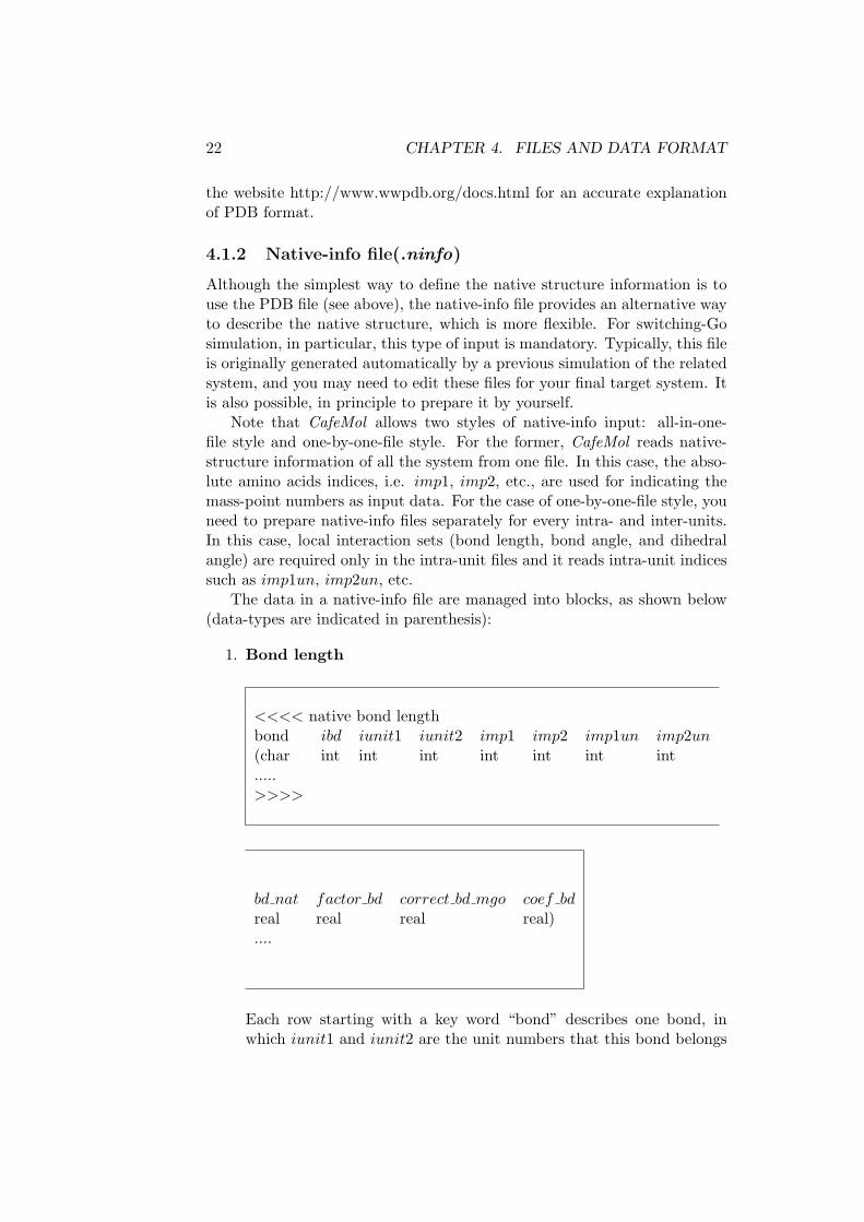
1. Bond length
<<<< native bond lengthbond ibd iunit1 iunit2 imp1 imp2 imp1un imp2un(char int int int int int int int.....>>>>
bd nat factor bd correct bd mgo coef bdreal real real real)....
Each row starting with a key word “bond” describes one bond, inwhich iunit1 and iunit2 are the unit numbers that this bond belongs

4.1. INPUT FILES 23
to (these two are always the same!), ibd is the bond number, imp1 andimp2 are the indices of N- and C-terminal amino acids, respectively,imp1un and imp2un are the intra-unit indices of the same two aminoacids, and bd nat is the native length of the bond. Typically, there arealso comment lines that start with asterisks (“∗”).
In the energy function of bond length, the coefficient is expressed as aproduct of a number of parameters:
coef bd(kcal/mol) = factor bd× correct bd mgo× cbd× energy unit protein
where factor bd = local unit × factor sec bd, local unit is overallweight of the local interaction for a unit, factor sec bd is the weightrelated to secondary structure (not implemented in current version),and correct bd mgo is for the weakening of local strain energy onsome particular sites when doing multiple-basin Go simulation. Bothfactor bd and correct bd mgo are site-specific parameters. cbd andenergy unit protein are constant coefficients of the energy function,for which you can find the explanation in Chapter 3.
As mentioned above, usage of columns is somewhat different betweenall-in-one-file style and one-by-one-file style. For the all-in-one-filecase, the 5th and the 6th columns are read as input data, while forthe one-by-one-file case, the 7th and the 8th columns are read as inputdata. This means that, in either case, there are some columns thatare not used. Still you should keep these unused columns as they are.Also noted is that for the one-by-one-file case, this block should be inthe intra-unit native-info files.
2. Bond angle
The data block for bond angle term is stored as following:
<<<< native bond anglesangl iba iunit1 iunit2 imp1 imp2 imp3 imp1un(char int int int int int int int.....>>>>
24 CHAPTER 4. FILES AND DATA FORMAT
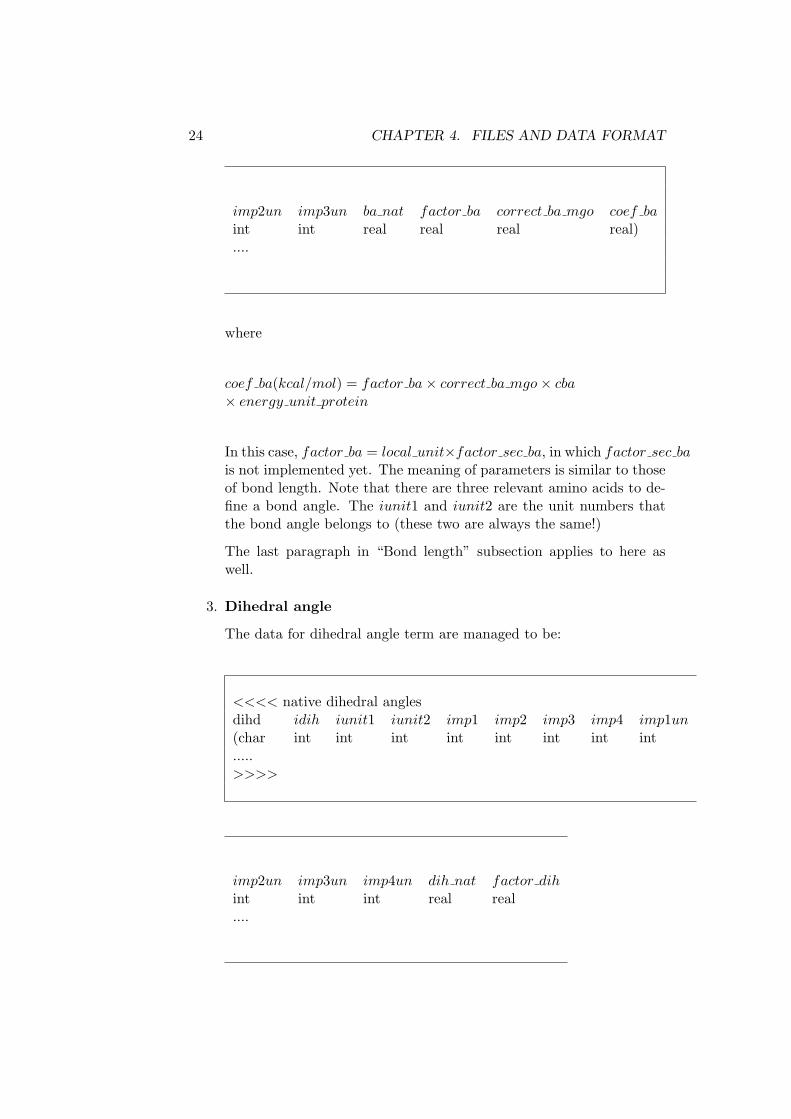
imp2un imp3un ba nat factor ba correct ba mgo coef baint int real real real real)....
where
coef ba(kcal/mol) = factor ba× correct ba mgo× cba× energy unit protein
In this case, factor ba = local unit×factor sec ba, in which factor sec bais not implemented yet. The meaning of parameters is similar to thoseof bond length. Note that there are three relevant amino acids to de-fine a bond angle. The iunit1 and iunit2 are the unit numbers thatthe bond angle belongs to (these two are always the same!)
The last paragraph in “Bond length” subsection applies to here aswell.
3. Dihedral angle
The data for dihedral angle term are managed to be:
<<<< native dihedral anglesdihd idih iunit1 iunit2 imp1 imp2 imp3 imp4 imp1un(char int int int int int int int int.....>>>>
imp2un imp3un imp4un dih nat factor dihint int int real real....

4.1. INPUT FILES 25
correct dih mgo coef dih 1 coef dih 3real real real)....
where
coef dih 1(kcal/mol) = factor dih× correct dih mgo× cdih 1× energy unit protein
and
coef dih 3(kcal/mol) = factor dih× correct dih mgo× cdih 3× energy unit protein.
are coefficients for the 2π-period and 23π-period terms of the energy
function, respectively. Similarly, you can find the meaning of eachparameter by looking up above explanation for the bond length. Notethat four amino acids are needed to define a dihedral angle.
The last paragraph in “Bond length” subsection applies to here aswell.
4. Native contact
The information of native contact is described as following:
<<<< native contactcontact icon iunit1 iunit2 imp1 imp2 imp1un imp2un(char int int int int int int int....>>>>
go nat factor go dummy mgo coef goreal real int real)....
26 CHAPTER 4. FILES AND DATA FORMAT
For most parameters, you can find counterparts in the case of localinteraction mentioned above. Here are some specialties:
coef go(kcal/mol) = factor go× dummy mgo× cgo1210× energy unit protein
where factor go = go unit × factor x, go unit is overall weight ofthe non-local interaction within a particular unit (or between a pairof units for the case of inter-unit contact), and factor x is a site-dependent weight which is not implemented in current version of CafeMol.dummy mgo is a boolean parameter indicating real contact (=1) ordummy-contact (=0). Please see Chapter 3 for detailed explana-tion. cgo1210 and energy unit protein are constant coefficients of theenergy function as mentioned above.
Again, we emphasize that CafeMol reads the absolute amino acids in-dices, i.e. imp1 and imp2 for the case of all-in-one-file style, while it readsintra-unit indices imp1un, and imp2un for the case of one-by-one-file style.
4.1.3 Input file (.inp)
Input file is the central file for users to configure a simulation. Please seeChapter 5 for a detailed explanation.
4.1.4 Parameter file (.para)
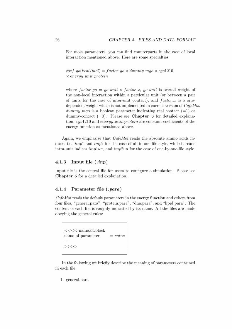
CafeMol reads the default parameters in the energy function and others fromfour files, “general.para”, “protein.para”, “dna.para”, and “lipid.para”. Thecontent of each file is roughly indicated by its name. All the files are madeobeying the general rules:
<<<< name of blockname of parameter = value.....>>>>
In the following we briefly describe the meaning of parameters containedin each file.
1. general.para
4.1. INPUT FILES 27
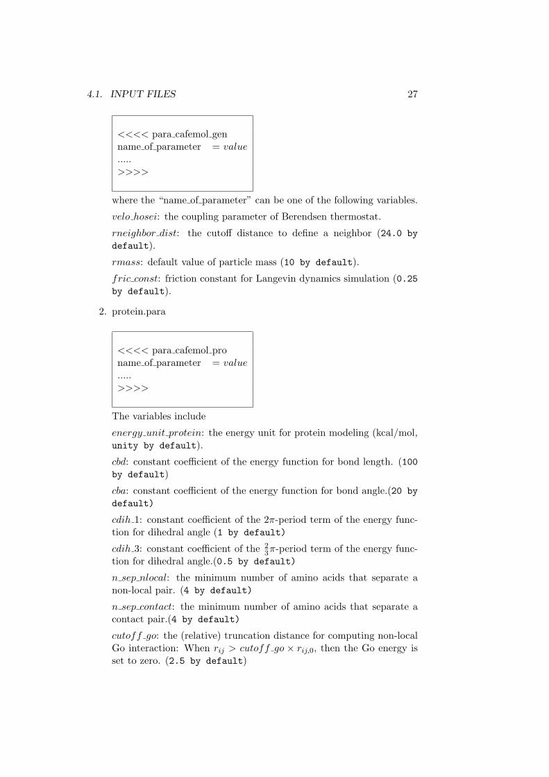
<<<< para cafemol genname of parameter = value.....>>>>
where the “name of parameter” can be one of the following variables.
velo hosei: the coupling parameter of Berendsen thermostat.
rneighbor dist: the cutoff distance to define a neighbor (24.0 by
default).
rmass: default value of particle mass (10 by default).
fric const: friction constant for Langevin dynamics simulation (0.25by default).
2. protein.para
<<<< para cafemol proname of parameter = value.....>>>>
The variables include
energy unit protein: the energy unit for protein modeling (kcal/mol,unity by default).
cbd: constant coefficient of the energy function for bond length. (100by default)
cba: constant coefficient of the energy function for bond angle.(20 by
default)
cdih 1: constant coefficient of the 2π-period term of the energy func-tion for dihedral angle (1 by default)
cdih 3: constant coefficient of the 23π-period term of the energy func-
tion for dihedral angle.(0.5 by default)
n sep nlocal: the minimum number of amino acids that separate anon-local pair. (4 by default)
n sep contact: the minimum number of amino acids that separate acontact pair.(4 by default)
cutoff go: the (relative) truncation distance for computing non-localGo interaction: When rij > cutoff go × rij,0, then the Go energy isset to zero. (2.5 by default)
28 CHAPTER 4. FILES AND DATA FORMAT
cutoff exvol: the (relative) truncation distance for computing non-local non-native repulsion: When rij > cutoff go× d, then the repul-sive energy is set to zero. (2.0 by default)
dfcontact: the cutoff distance to define the native contact (6.5 by
default).
cgo1210: constant coefficient εgo of the energy function for non-localGo interaction.(0.3 by default)
cdist rep12: reference distance d in the non-native repulsive interac-tion of Clementi et al.’s Go model. (4 by default)
crep12: constant coefficient εev in the non-native repulsive interactionof Clementi et al.’s Go model. (0.2 by default)
3. dna.para
to be added
4. lipid.para
to be added
Note that the default parameter files are placed under the directory“./para” and we recommend that they remain unchanged.
4.2 Output files
4.2.1 PDB file (.pdb)
The output PDB file can be used as a restart file for a new simulation.Please access http://www.wwpdb.org/docs.html for the description of thisformat.
4.2.2 CARD coordinate (.crd) and velocity (.velo)
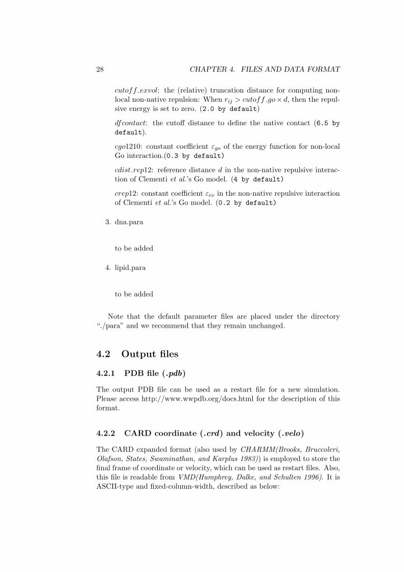
The CARD expanded format (also used by CHARMM(Brooks, Bruccoleri,Olafson, States, Swaminathan, and Karplus 1983)) is employed to store thefinal frame of coordinate or velocity, which can be used as restart files. Also,this file is readable from VMD(Humphrey, Dalke, and Schulten 1996). It isASCII-type and fixed-column-width, described as below:
4.2. OUTPUT FILES 29
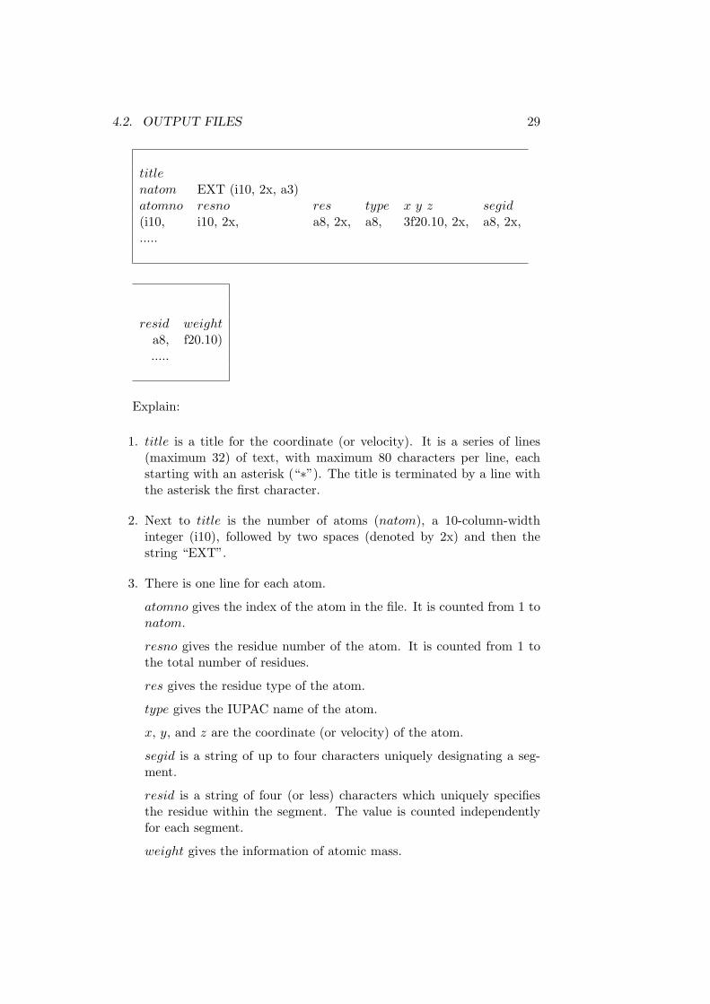
titlenatom EXT (i10, 2x, a3)atomno resno res type x y z segid(i10, i10, 2x, a8, 2x, a8, 3f20.10, 2x, a8, 2x,.....
resid weighta8, f20.10).....
Explain:
1. title is a title for the coordinate (or velocity). It is a series of lines(maximum 32) of text, with maximum 80 characters per line, eachstarting with an asterisk (“∗”). The title is terminated by a line withthe asterisk the first character.
2. Next to title is the number of atoms (natom), a 10-column-widthinteger (i10), followed by two spaces (denoted by 2x) and then thestring “EXT”.
3. There is one line for each atom.
atomno gives the index of the atom in the file. It is counted from 1 tonatom.
resno gives the residue number of the atom. It is counted from 1 tothe total number of residues.
res gives the residue type of the atom.
type gives the IUPAC name of the atom.
x, y, and z are the coordinate (or velocity) of the atom.
segid is a string of up to four characters uniquely designating a seg-ment.
resid is a string of four (or less) characters which uniquely specifiesthe residue within the segment. The value is counted independentlyfor each segment.
weight gives the information of atomic mass.

30 CHAPTER 4. FILES AND DATA FORMAT
4.2.3 DCD coordinate (.dcd) and velocity (.vdcd)
CafeMol adopts DCD format (also used by CHARMM(Brooks, Brucco-leri, Olafson, States, Swaminathan, and Karplus 1983) and NAMD(Phillips,Braun, Wang, Gumbart, Tajkhorshid, Villa, Chipot, Skeel, Kale, and Schulten2005). This format is readable by VMD(Humphrey, Dalke, and Schulten1996) so that one can watch the simulation movie) to save trajectory inbinary. (GNU compiler is not supported.) The format is described as fol-lowing:
blocksize1 hdr nset istrt nsavc nstep null(int char∗4 int int int int int∗4)
natom− nfreat delta null version blocksize1(int real int∗9 int int )
blocksize2 ntitle title blocksize2(int int char(80)∗ntitle int)
blocksize3 natom blocksize3(int int int)
blocksize4 x blocksize4(int real∗natom int)
blocksize5 y blocksize5(int real∗natom int)
blocksize6 z blocksize6(int real∗natom int)
Explain:
1. There are six types of blocks in the whole file starting and endingwith blocksize for each, containing simulation information, the title,the total number of atoms, and x-, y-, and z-coordinate (or velocity), respectively. The blocksize means the total bytes for a particularblock. For example, the size of the block 1 (blocksize1) must alwaysbe 84.
2. The first block describes parameters of simulation and it contains 8values plus 13 trivial zeros.
hdr is the header of the file, and it can be either “CORD” or “VELD”,for coordinate or velocity, respectively.
nset means the total number of frames in the trajectory.
4.2. OUTPUT FILES 31
istrt indicates the starting time-step. In most cases it is equal to 1,but it may also be larger than 1 when a continuous stimulation isperformed for a previous one.
nsavc is the frequency to save coordinate (or velocity) in the simula-tion.
nstep is the total number of time-steps of the simulation.
null means these positions are reserved. In this case it is an array offour integer zeros.
natom − nfreat means the number of free atoms (corresponding tofixed atoms in some cases). Currently it is set to be zero.
delta saves the step-size of the simulation.
null is an array of nine integer zeros.
version is set to be 24, which means we pretend to be a CHARMM24format.
3. The second block describes the title.
ntitle is the number of title lines, and it should be less than 33.
title is the real content of the title, which should be managed into singleor multiple lines with each line containing exactly 80 characters.
4. The third block saves simply the total number of atoms (natom) inthe trajectory.
5. Block No. 4-6 save the coordinate (or velocity).
x, y, and z are coordinate (or velocity) with respect to x-, y-, andz-axis, respectively.
Note that block No. 3-6 are repeated for a trajectory.
4.2.4 Movie file (.movie)
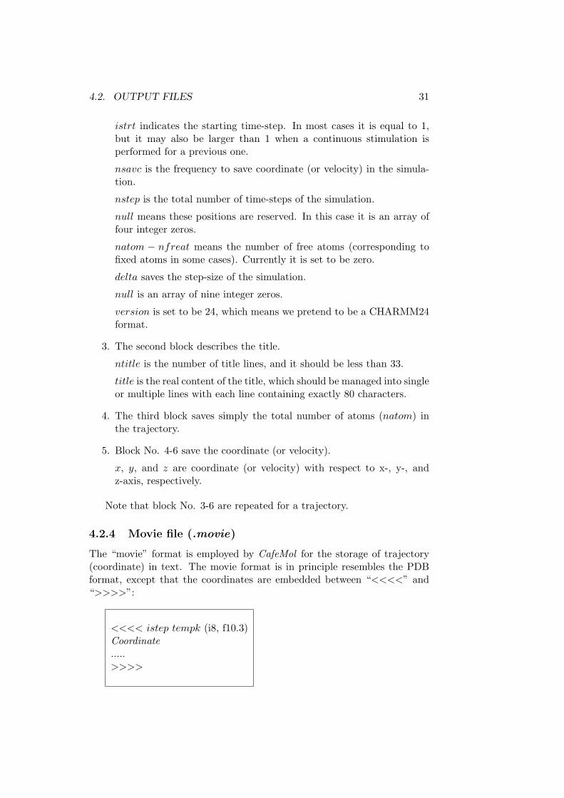
The “movie” format is employed by CafeMol for the storage of trajectory(coordinate) in text. The movie format is in principle resembles the PDBformat, except that the coordinates are embedded between “<<<<” and“>>>>”:
<<<< istep tempk (i8, f10.3)Coordinate.....>>>>
32 CHAPTER 4. FILES AND DATA FORMAT
where istep is the current time-step, and tempk is the temperature. Thecoordinates are collected with respect to unit, and for each unit the dataare embedded in a lower level block:
<< protein iunit (i3)Coordinate.....>>
where iunit represents the unit number.
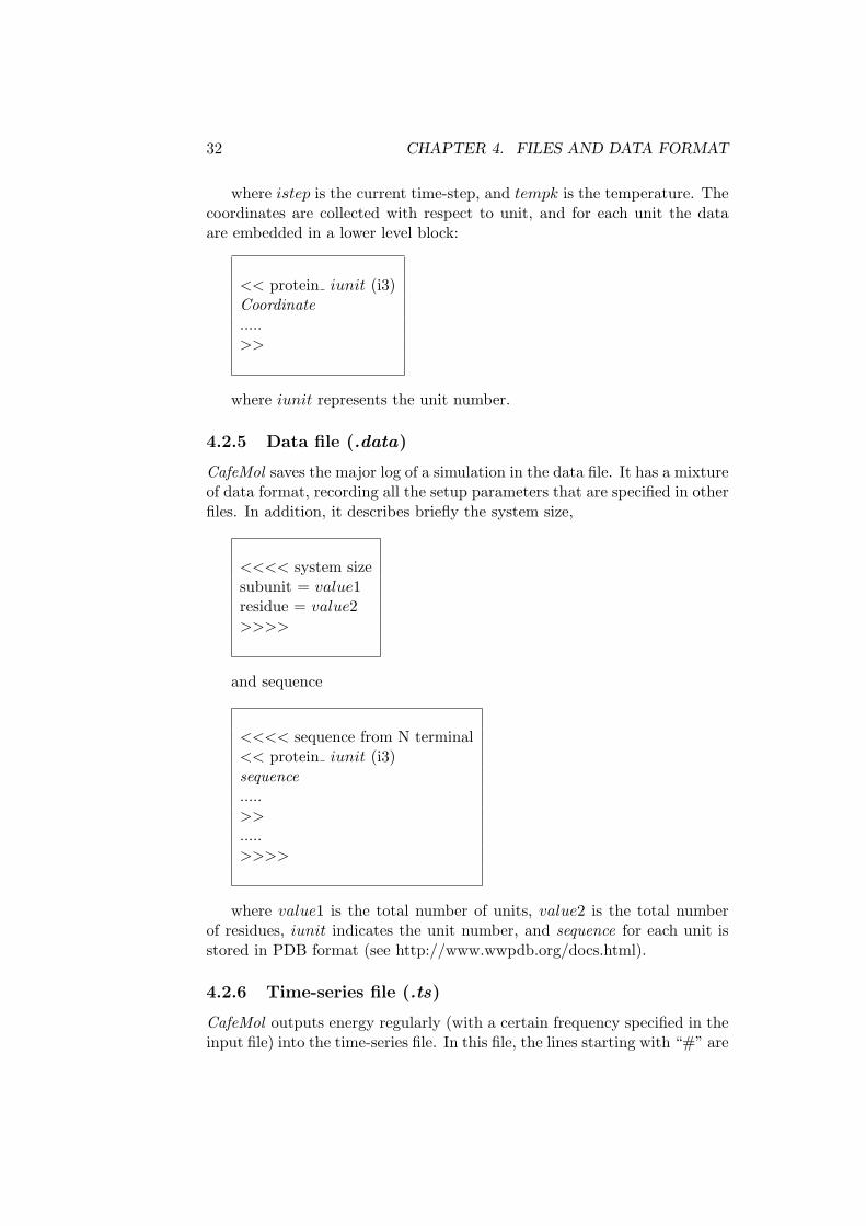
4.2.5 Data file (.data)
CafeMol saves the major log of a simulation in the data file. It has a mixtureof data format, recording all the setup parameters that are specified in otherfiles. In addition, it describes briefly the system size,
<<<< system sizesubunit = value1residue = value2>>>>
and sequence
<<<< sequence from N terminal<< protein iunit (i3)sequence.....>>.....>>>>
where value1 is the total number of units, value2 is the total numberof residues, iunit indicates the unit number, and sequence for each unit isstored in PDB format (see http://www.wwpdb.org/docs.html).
4.2.6 Time-series file (.ts)
CafeMol outputs energy regularly (with a certain frequency specified in theinput file) into the time-series file. In this file, the lines starting with “#” are

4.2. OUTPUT FILES 33
comments (so that it is skipped in gnuplot), and the others are time-seriesof some basic quantities, of which formats depend on simulations performed.It is a plain text format.
For the case that the system only contains simple Go models, the outputlooks like:
#unit step tempk radg etot velet qscore local go repul( int real real real real real)# all (int real real real real real real real real)# 1 (int real real real real real real real real)... ...
There is one non-comment line for each time-step reporting the results ofsome order parameters and total energy terms of the whole system. For thisline, variables are explained as following: step is the time-step, tempk is thetemperature, radg is the radius of gyration, etot is the total energy, velet isthe kinetic energy, and qscore is the fraction of native contacts.
The following comments lines report the information for each unit, aswell as its sum. In addition to the columns described above,.local is theenergy of local interaction, go is the energy of non-local Go interaction,and repul is the energy of repulsive interaction. Moreover, when “bridge”,“pulling”, “anchor”, or “in box” options are turned on (See Chapter 5), thecorresponding energy terms for these will be printed as additional columns(It is noted that etot in the non-comment line includes these energy terms).
For the case that the system contains multiple-basin Go model, the filelooks like:
# step tempk radg etot velet 1sys#unit step tempk radg etot velet qscore( int real real real real i3, a3# all (int real real real real real# 1a (int real real real real real.....

34 CHAPTER 4. FILES AND DATA FORMAT
ch a− b ... coef a qsco a estate a coef b qscore b estate b ...local go repulreal ... real real real real real real ...real real real)real real real).....
The third line is the summary data for each time-step, of which labels aregiven in the first comment line: the columns from step to velet describethe whole system in the same way as those in single Go case, while the fol-lowing columns describe data for each multiple-basin (MB) system (Systemnumbers are indicated by digits and state numbers by lowercase alphabets).Several columns from “1sys”, for example, describes results for the first MBsystem. Within the description of each MB system, the output for eachstate are also shown in order. ch a − b is the order parameter χ definedbetween states a and b. For system of more than two basins, the number ofch is larger than one, and they are output sequentially in this file. Then,coef a , qsco a, and estate a are the force coefficient, Q-score (the fractionof native contact), and energy, respectively, for state a.
Then, from the fourth line, as in the case of simple Go simulation, theinformation of each unit, as well as its sum is output as comment lines,of which labels are given in the second line. All variables have the samemeaning as the case of simple Go simulation explained above.
4.2.7 Native-info file(.ninfo)
The output native-info file is essentially the same format to the input native-info file. Please see 4.1.2 for a reference of such file format.
Chapter 5
Input file: How to make
5.1 General rules of input files
First of all, we expect (hope!) that CafeMol runs appropriately only whenan input file is prepared consistently throughout the file. When you use aninconsistent input file, CafeMol is not necessarily kind enough to stop withan error message, but quite often still runs and provides some results, butthose results are most likely meaningless. It is your responsibility to makea consistent input file!. You should read through the manual before doingsimulations.
The input file of CafeMol uses general rules. Knowledge of them will beessential to write and understand input files.
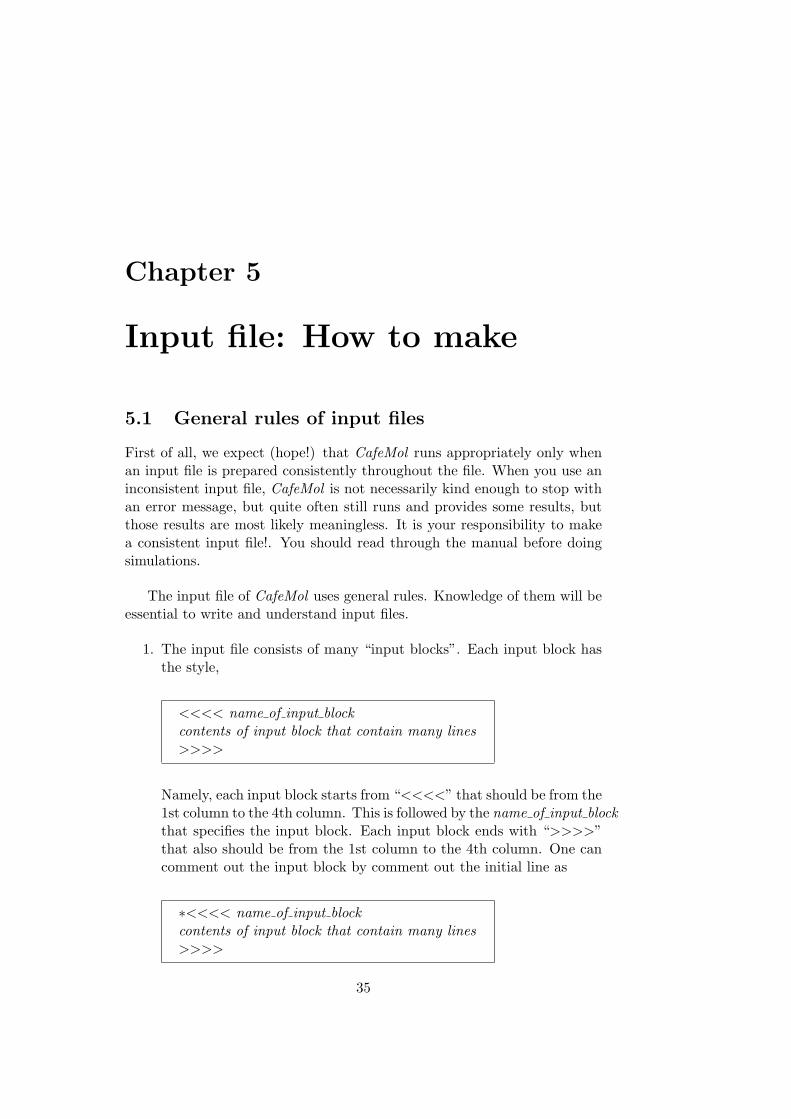
1. The input file consists of many “input blocks”. Each input block hasthe style,
<<<< name of input blockcontents of input block that contain many lines>>>>
Namely, each input block starts from “<<<<” that should be from the1st column to the 4th column. This is followed by the name of input blockthat specifies the input block. Each input block ends with “>>>>”that also should be from the 1st column to the 4th column. One cancomment out the input block by comment out the initial line as
∗<<<< name of input blockcontents of input block that contain many lines>>>>
35
36 CHAPTER 5. INPUT FILE: HOW TO MAKE
The above input block is entirely ignored.
For every CafeMol input files, several input blocks are required, andothers are optional. Orders of these input blocks are not essential.You can order them freely.
The input file is completely made of input blocks. Any message outof blocks are just ignored.
Within an input block, many lines are to be written. Orders of linesare free.
2. Lines that have “∗” in the 1st column are taken as comments. Blanklines are also ignored.
3. There are only two styles of lines in the input file, each of which willbe described in 4 and 5.
4. Many lines in input files contain the style,
name of parameter = value
For this, the style is quite flexible. Name of parameter can start fromany column. Between name of parameter and =, and between = andvalue, any length of space (including zero) is allowed. However, thereis a length limit for both left and right hand sides. value should be nolonger than 64 characters.
5. Many lines in input files starts from the UPPERCASE words.
PARAMETER ,,,,,
For this uppercase word, one has to write it from the 1st column. Onthese lines, usually up to the 1st space, the format is quite rigid.
5.2 <<<< filenames (required)
This input block sets paths, input and output filenames, and output dataformats.
The following line defines the directory where output data are saved.
path = directory (default “./data”)

5.2. <<<< FILENAMES (REQUIRED) 37
The next line sets the output file names up to the suffix.
filename = name of file (required)
The following specifies what types of output files you are requesting to get.
OUTPUT name of formats to be output (optional)
Out of 6 available formats, you can write any numbers of the formats. The 6available formats pdb, crd, velo, movie, dcd, and vdcd. The former 3 savesdata only about 10 times in a run and are used primarily for restart. Onthe other hand, the latter 3 saves data much more frequently and can beused for trajectory analysis and making movie.
1. pdb; PDB file format for (coordinate)
2. crd; CARD file format for (coordinate). This allows one to save longerdigits coordinates than the PDB format. For very large systems, thisformat is required.
3. velo; CARD file format for (velocity).
4. movie; PDB file format for trajectory (coordinate)
5. dcd; DCD file format for trajectory (coordinate), which can be putinto VMD for watching movie. (CafeMol compiled by GNU compilercan not run with this option.)
6. vdcd; DCD file format for trajectory (velocity), which may not beused very often. (CafeMol compiled by GNU compiler can not runwith this option.)
The next line defines the directory where the native (reference) structuresare prepared.
path pdb = directory (default “./pdb”)
The next line defines the directory where the initial structures are prepared.
path ini = directory (default “./pdb”)
38 CHAPTER 5. INPUT FILE: HOW TO MAKE
The following defines the directory where the native (reference) informationis prepared.
path natinfo = directory (default “./ninfo”)
An example of this input block is
<<<< filenamespath = ./datafilename = cafemol mgo 1chainOUTPUT crd velo dcd pdbpath pdb = ./pdbpath ini = ./pdbpath natinfo = ./ninfo>>>>
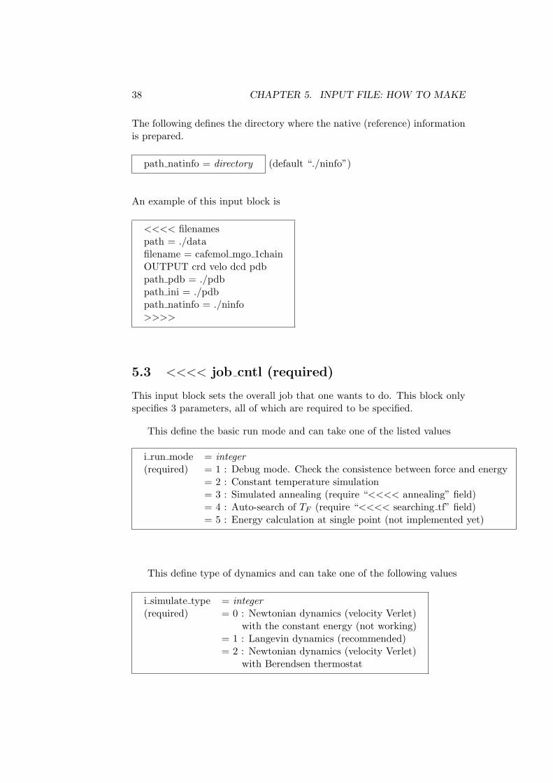
5.3 <<<< job cntl (required)
This input block sets the overall job that one wants to do. This block onlyspecifies 3 parameters, all of which are required to be specified.
This define the basic run mode and can take one of the listed values
i run mode = integer(required) = 1 : Debug mode. Check the consistence between force and energy
= 2 : Constant temperature simulation= 3 : Simulated annealing (require “<<<< annealing” field)= 4 : Auto-search of TF (require “<<<< searching tf” field)= 5 : Energy calculation at single point (not implemented yet)
This define type of dynamics and can take one of the following values
i simulate type = integer(required) = 0 : Newtonian dynamics (velocity Verlet)
with the constant energy (not working)= 1 : Langevin dynamics (recommended)= 2 : Newtonian dynamics (velocity Verlet)
with Berendsen thermostat
5.4. <<<< UNIT AND STATE (REQUIRED) 39
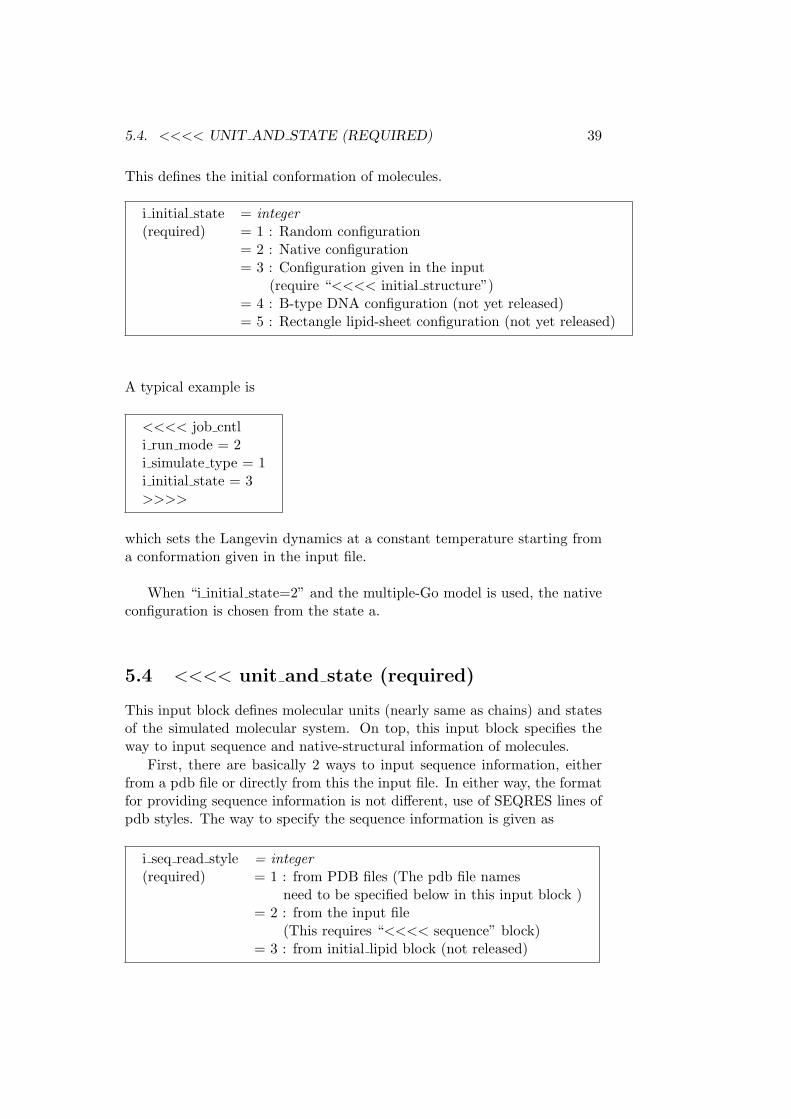
This defines the initial conformation of molecules.
i initial state = integer(required) = 1 : Random configuration
= 2 : Native configuration= 3 : Configuration given in the input
(require “<<<< initial structure”)= 4 : B-type DNA configuration (not yet released)= 5 : Rectangle lipid-sheet configuration (not yet released)
A typical example is
<<<< job cntli run mode = 2i simulate type = 1i initial state = 3>>>>
which sets the Langevin dynamics at a constant temperature starting froma conformation given in the input file.
When “i initial state=2” and the multiple-Go model is used, the nativeconfiguration is chosen from the state a.
5.4 <<<< unit and state (required)
This input block defines molecular units (nearly same as chains) and statesof the simulated molecular system. On top, this input block specifies theway to input sequence and native-structural information of molecules.
First, there are basically 2 ways to input sequence information, eitherfrom a pdb file or directly from this the input file. In either way, the formatfor providing sequence information is not different, use of SEQRES lines ofpdb styles. The way to specify the sequence information is given as
i seq read style = integer(required) = 1 : from PDB files (The pdb file names
need to be specified below in this input block )= 2 : from the input file
(This requires “<<<< sequence” block)= 3 : from initial lipid block (not released)
40 CHAPTER 5. INPUT FILE: HOW TO MAKE
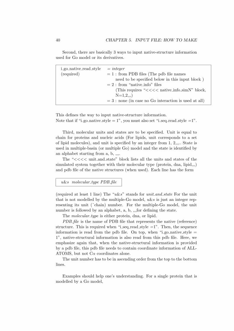
Second, there are basically 3 ways to input native-structure informationused for Go model or its derivatives.
i go native read style = integer(required) = 1 : from PDB files (The pdb file names
need to be specified below in this input block )= 2 : from “native info” files
(This requires “<<<< native info simN” block,N=1,2,,,)
= 3 : none (in case no Go interaction is used at all)
This defines the way to input native-structure information.
Note that if “i go native style = 1”, you must also set “i seq read style =1”.
Third, molecular units and states are to be specified. Unit is equal tochain for proteins and nucleic acids (For lipids, unit corresponds to a setof lipid molecules), and unit is specified by an integer from 1, 2,,,.. State isused in multiple-basin (or multiple Go) model and the state is identified byan alphabet starting from a, b, ,,,.
The “<<<< unit and state” block lists all the units and states of thesimulated system together with their molecular type (protein, dna, lipid,,,)and pdb file of the native structures (when used). Each line has the form
u&s molecular type PDB file
(required at least 1 line) The “u&s” stands for unit and state For the unitthat is not modelled by the multiple-Go model, u&s is just an integer rep-resenting its unit (˜chain) number. For the multiple-Go model, the unitnumber is followed by an alphabet, a, b, ,,,for defining the state.
The molecular type is either protein, dna, or lipid.
PDB file is the name of PDB file that represents the native (reference)structure. This is required when “i seq read style =1”. Then, the sequenceinformation is read from the pdb file. On top, when “i go native style =1”, native-structural information is also read from this pdb file. Here, weemphasize again that, when the native-structural information is providedby a pdb file, this pdb file needs to contain coordinate information of ALL-ATOMS, but not Cα coordinates alone.
The unit number has to be in ascending order from the top to the bottomlines.
Examples should help one’s understanding. For a single protein that ismodelled by a Go model,
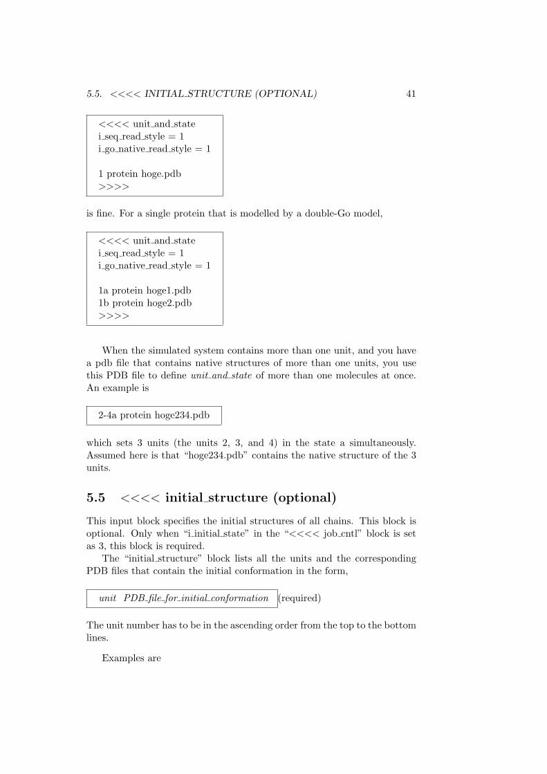
5.5. <<<< INITIAL STRUCTURE (OPTIONAL) 41
<<<< unit and statei seq read style = 1i go native read style = 1
1 protein hoge.pdb>>>>
is fine. For a single protein that is modelled by a double-Go model,
<<<< unit and statei seq read style = 1i go native read style = 1
1a protein hoge1.pdb1b protein hoge2.pdb>>>>
When the simulated system contains more than one unit, and you havea pdb file that contains native structures of more than one units, you usethis PDB file to define unit and state of more than one molecules at once.An example is
2-4a protein hoge234.pdb
which sets 3 units (the units 2, 3, and 4) in the state a simultaneously.Assumed here is that “hoge234.pdb” contains the native structure of the 3units.
5.5 <<<< initial structure (optional)
This input block specifies the initial structures of all chains. This block isoptional. Only when “i initial state” in the “<<<< job cntl” block is setas 3, this block is required.
The “initial structure” block lists all the units and the correspondingPDB files that contain the initial conformation in the form,
unit PDB file for initial conformation (required)
The unit number has to be in the ascending order from the top to the bottomlines.
Examples are

42 CHAPTER 5. INPUT FILE: HOW TO MAKE
<<<< initial structure1 hoge1.pdb2 hoge2.pdb>>>>
Note that you should not put the state id, a or b after the unit number evenif you are using multiple-Go model for some units; The initial structureshould be unique! As before, CafeMol accepts the assignment of more thanone unit simultaneously, like the form
<<<< initial structure1-2 hoge12.pdb>>>>
Of course, “hoge12.pdb” should contain the initial structures of the units 1and 2.
5.6 <<<< initial lipid (not implemented)
This input block is required only when the simulation system contains lipid.CafeMol has a simple and automatic lipid bilayer generator that places lipidmolecules with equal space in transverse and longitudinal directions to makea 2D square bilayer. This block is to specify some parameters needed togenerate lipid bilayer.
nmp transverse lipid =integer (required)nmp longitudinal lipid =integer (required)grid size lipid =real (required)
where the first two lines define the number of lipid molecules in x- andy-directions. The last line sets the in-plane distance between neighboringlipids in A.
5.7 <<<< energy function (required)
This input block sets the energy function used for each of simulating chains.This mostly sets the non-local interactions of Go model and multiple-Gomodel. The local part has no option except the choice of parameters, andthus no input line exists for the local interaction. This block consists of afew types of lines.
First, for each pair of unit and states, you need to define the type of
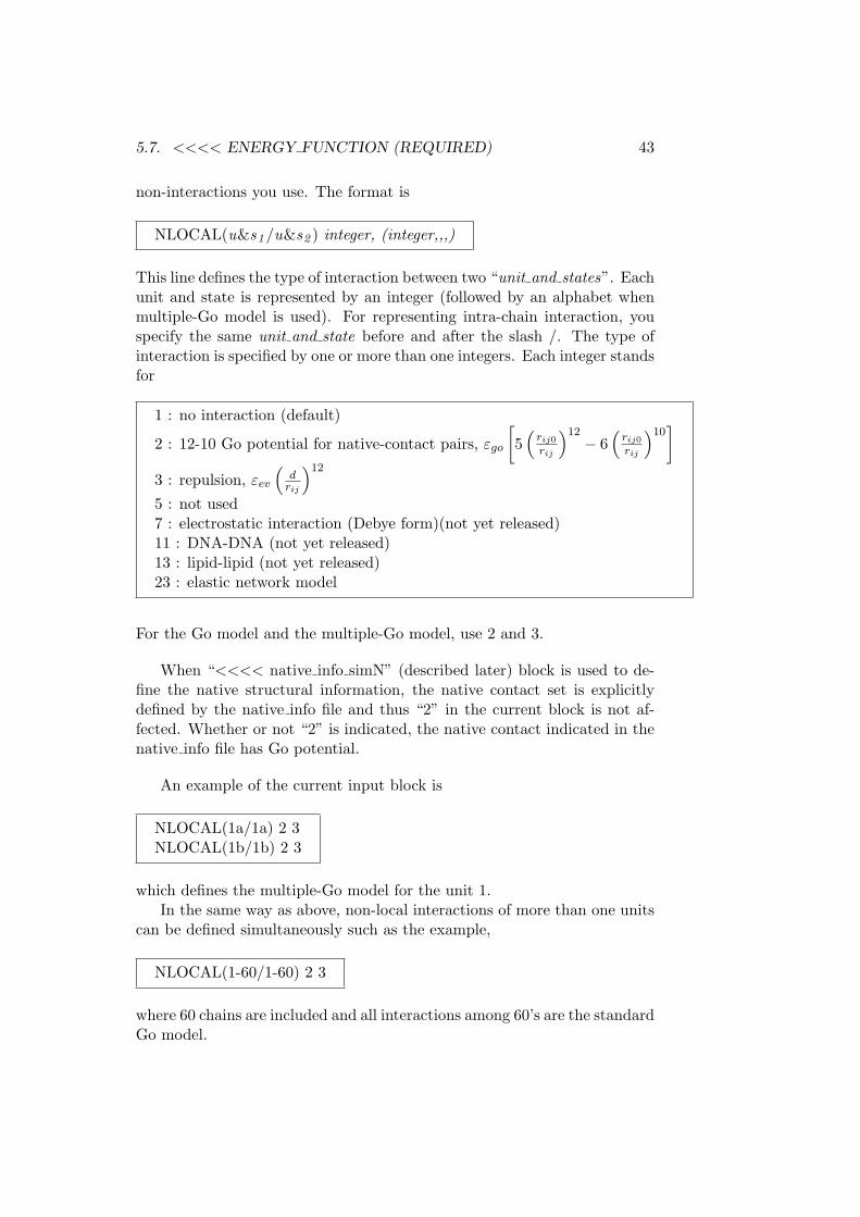
5.7. <<<< ENERGY FUNCTION (REQUIRED) 43
non-interactions you use. The format is
NLOCAL(u&s1/u&s2 ) integer, (integer,,,)
This line defines the type of interaction between two “unit and states”. Eachunit and state is represented by an integer (followed by an alphabet whenmultiple-Go model is used). For representing intra-chain interaction, youspecify the same unit and state before and after the slash /. The type ofinteraction is specified by one or more than one integers. Each integer standsfor
1 : no interaction (default)
2 : 12-10 Go potential for native-contact pairs, εgo
[
5(
rij0
rij
)12− 6
(
rij0
rij
)10]
3 : repulsion, εev
(
drij
)12
5 : not used7 : electrostatic interaction (Debye form)(not yet released)11 : DNA-DNA (not yet released)13 : lipid-lipid (not yet released)23 : elastic network model
For the Go model and the multiple-Go model, use 2 and 3.
When “<<<< native info simN” (described later) block is used to de-fine the native structural information, the native contact set is explicitlydefined by the native info file and thus “2” in the current block is not af-fected. Whether or not “2” is indicated, the native contact indicated in thenative info file has Go potential.
An example of the current input block is
NLOCAL(1a/1a) 2 3NLOCAL(1b/1b) 2 3
which defines the multiple-Go model for the unit 1.In the same way as above, non-local interactions of more than one units
can be defined simultaneously such as the example,
NLOCAL(1-60/1-60) 2 3
where 60 chains are included and all interactions among 60’s are the standardGo model.
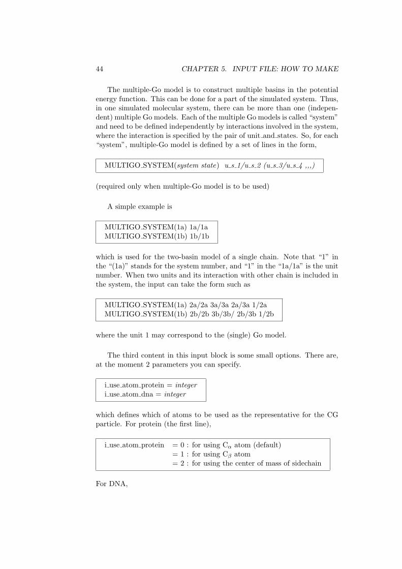
44 CHAPTER 5. INPUT FILE: HOW TO MAKE
The multiple-Go model is to construct multiple basins in the potentialenergy function. This can be done for a part of the simulated system. Thus,in one simulated molecular system, there can be more than one (indepen-dent) multiple Go models. Each of the multiple Go models is called “system”and need to be defined independently by interactions involved in the system,where the interaction is specified by the pair of unit and states. So, for each“system”, multiple-Go model is defined by a set of lines in the form,
MULTIGO SYSTEM(system state) u s 1/u s 2 (u s 3/u s 4 ,,,)
(required only when multiple-Go model is to be used)
A simple example is
MULTIGO SYSTEM(1a) 1a/1aMULTIGO SYSTEM(1b) 1b/1b
which is used for the two-basin model of a single chain. Note that “1” inthe “(1a)” stands for the system number, and “1” in the “1a/1a” is the unitnumber. When two units and its interaction with other chain is included inthe system, the input can take the form such as
MULTIGO SYSTEM(1a) 2a/2a 3a/3a 2a/3a 1/2aMULTIGO SYSTEM(1b) 2b/2b 3b/3b/ 2b/3b 1/2b
where the unit 1 may correspond to the (single) Go model.
The third content in this input block is some small options. There are,at the moment 2 parameters you can specify.
i use atom protein = integeri use atom dna = integer
which defines which of atoms to be used as the representative for the CGparticle. For protein (the first line),
i use atom protein = 0 : for using Cα atom (default)= 1 : for using Cβ atom= 2 : for using the center of mass of sidechain
For DNA,
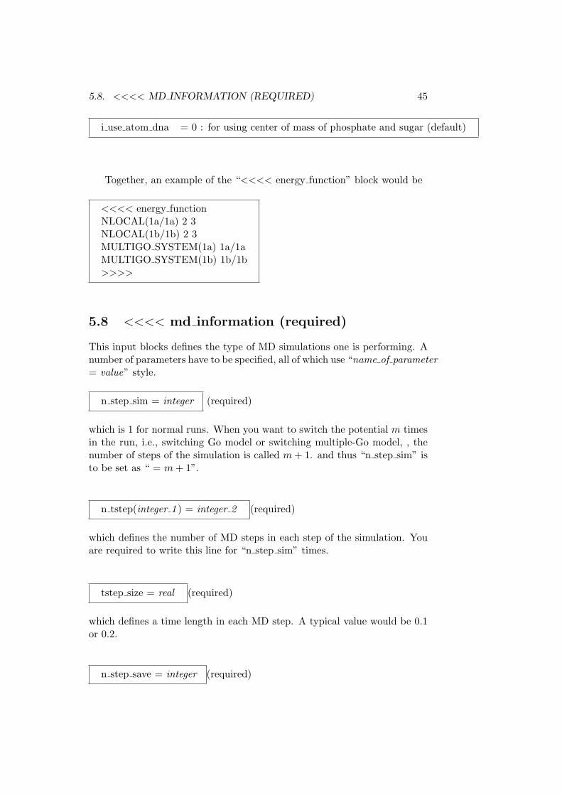
5.8. <<<< MD INFORMATION (REQUIRED) 45
i use atom dna = 0 : for using center of mass of phosphate and sugar (default)
Together, an example of the “<<<< energy function” block would be
<<<< energy functionNLOCAL(1a/1a) 2 3NLOCAL(1b/1b) 2 3MULTIGO SYSTEM(1a) 1a/1aMULTIGO SYSTEM(1b) 1b/1b>>>>
5.8 <<<< md information (required)
This input blocks defines the type of MD simulations one is performing. Anumber of parameters have to be specified, all of which use “name of parameter= value” style.
n step sim = integer (required)
which is 1 for normal runs. When you want to switch the potential m timesin the run, i.e., switching Go model or switching multiple-Go model, , thenumber of steps of the simulation is called m + 1. and thus “n step sim” isto be set as “ = m + 1”.
n tstep(integer 1 ) = integer 2 (required)
which defines the number of MD steps in each step of the simulation. Youare required to write this line for “n step sim” times.
tstep size = real (required)
which defines a time length in each MD step. A typical value would be 0.1or 0.2.
n step save = integer (required)
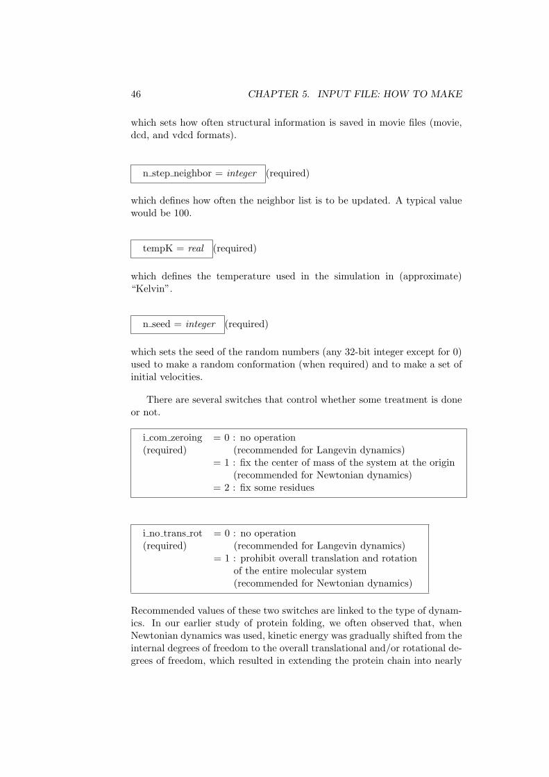
46 CHAPTER 5. INPUT FILE: HOW TO MAKE
which sets how often structural information is saved in movie files (movie,dcd, and vdcd formats).
n step neighbor = integer (required)
which defines how often the neighbor list is to be updated. A typical valuewould be 100.
tempK = real (required)
which defines the temperature used in the simulation in (approximate)“Kelvin”.
n seed = integer (required)
which sets the seed of the random numbers (any 32-bit integer except for 0)used to make a random conformation (when required) and to make a set ofinitial velocities.
There are several switches that control whether some treatment is doneor not.
i com zeroing = 0 : no operation(required) (recommended for Langevin dynamics)
= 1 : fix the center of mass of the system at the origin(recommended for Newtonian dynamics)
= 2 : fix some residues
i no trans rot = 0 : no operation(required) (recommended for Langevin dynamics)
= 1 : prohibit overall translation and rotationof the entire molecular system(recommended for Newtonian dynamics)
Recommended values of these two switches are linked to the type of dynam-ics. In our earlier study of protein folding, we often observed that, whenNewtonian dynamics was used, kinetic energy was gradually shifted from theinternal degrees of freedom to the overall translational and/or rotational de-grees of freedom, which resulted in extending the protein chain into nearly

5.8. <<<< MD INFORMATION (REQUIRED) 47
straight line (by this, with a small angular momentum, kinetic energy of ro-tation increases radically) and freezing the internal motion. This occurredbecause of some small non-zero angular momentum and thus it is highlyrecommended to prohibit overall translational and rotational motions whenthe Newtonian dynamics is used. Since the translational motion is inhibited,it is easier for the analysis to move the center of mass of the system to theorigin of the space coordinate. On the other hand, Langevin dynamics doesnot have this problem and thus it is recommended not to use this kind oftreatment.
i in box = 0 ; no operation (default)= 1 : put the entire system into a box of rectangular solid
(requires the input block “<<<< in box”)
i del int = 0 : no operation (default)= 1 : delete some interactions in a particular range
(requires the input block “<<<< del interaction”)
This is particularly useful when some portions of a protein is disordered andthus is not seen in the PDB structure, but you still need to include theseresidues in the simulation. In this case, you may model these disorderedloops by some software and use the modelled structure as the native. Yet,you do not want to rely heavily on these loop structure in the model. Then,it is recommended to delete Go-like interactions that are dependent on themodelled loops.
i redef para = 0 : no operation (default)= 1 : re-define some default parameters
(requires the input block “<<<< redefine para”)
Use of this option is suitable mostly for advanced users. What kinds ofparameters can be re-defined is not well documented and thus you need toread the source code for full use of this option.
i energy para = 0 : no operation (default)= 1 : re-scale some energy parameters
(requires the input block “<<<< energy para”
This is used when you want to re-scale strength of some interactions for some
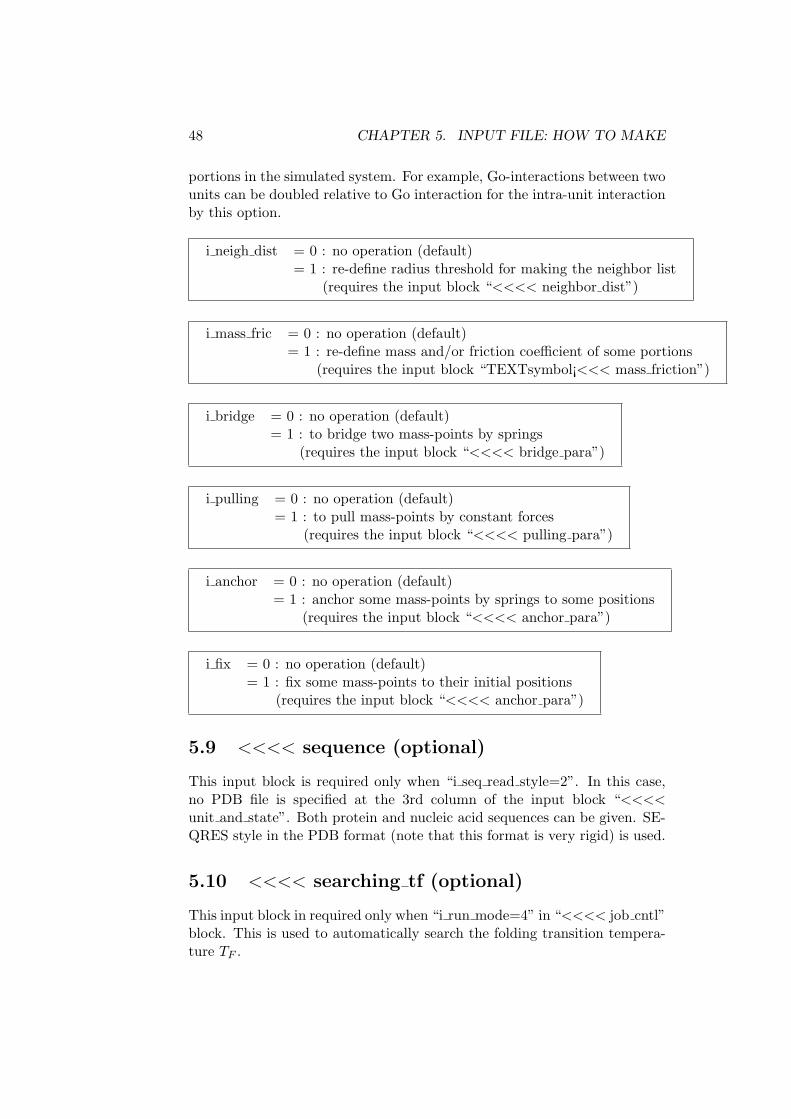
48 CHAPTER 5. INPUT FILE: HOW TO MAKE
portions in the simulated system. For example, Go-interactions between twounits can be doubled relative to Go interaction for the intra-unit interactionby this option.
i neigh dist = 0 : no operation (default)= 1 : re-define radius threshold for making the neighbor list
(requires the input block “<<<< neighbor dist”)
i mass fric = 0 : no operation (default)= 1 : re-define mass and/or friction coefficient of some portions
(requires the input block “TEXTsymbol¡<<< mass friction”)
i bridge = 0 : no operation (default)= 1 : to bridge two mass-points by springs
(requires the input block “<<<< bridge para”)
i pulling = 0 : no operation (default)= 1 : to pull mass-points by constant forces
(requires the input block “<<<< pulling para”)
i anchor = 0 : no operation (default)= 1 : anchor some mass-points by springs to some positions
(requires the input block “<<<< anchor para”)
i fix = 0 : no operation (default)= 1 : fix some mass-points to their initial positions
(requires the input block “<<<< anchor para”)
5.9 <<<< sequence (optional)
This input block is required only when “i seq read style=2”. In this case,no PDB file is specified at the 3rd column of the input block “<<<<unit and state”. Both protein and nucleic acid sequences can be given. SE-QRES style in the PDB format (note that this format is very rigid) is used.
5.10 <<<< searching tf (optional)
This input block in required only when “i run mode=4” in “<<<< job cntl”block. This is used to automatically search the folding transition tempera-ture TF .

5.11. <<<< ANNEALING (OPTIONAL) 49
tempK upper = real (required)tempK lower = real (required, should be smaller than tempK upper)
These two temperatures provide the upper and lower bounds of the TF .
5.11 <<<< annealing (optional)
This input block in required only when “i run mode=3” in “<<<< job cntl”block. This is to specify the parameters in the simulated annealing run.Parameters to be specified are the following three.
tempK init = real (required)tempK last = real (required, should be smaller than tempK init)itime change = integer (required)
By this, the simulated run starts with the temperature =“tempK init” (inKelvin) and ends with the temperature =“tempK last”. During the MDsteps, the temperature is linearly decreased “itime change” times.
5.12 <<<< multiple go (optional)
This is to specify parameters needed for multiple Go model simulations andthus is required only when “MULTIGO SYSTEM” lines exist in “<<<<energy function”.
bdemax mgo = real (required)
which sets the upper limit of the change in bond stretching energy ǫb,max(in“kcal/mol/A2” unit). A typical value is 100.
baemax mgo = real (required)
which sets the upper limit of the change in bond angle energy ǫθ,max(in“kcal/mol/radian2” unit). A typical value is 1.
dihemax mgo = real (required)
which sets the upper limit of the change in dihedral angle energy ǫφ,max(in“kcal/mol” unit). A typical value is 0.5.
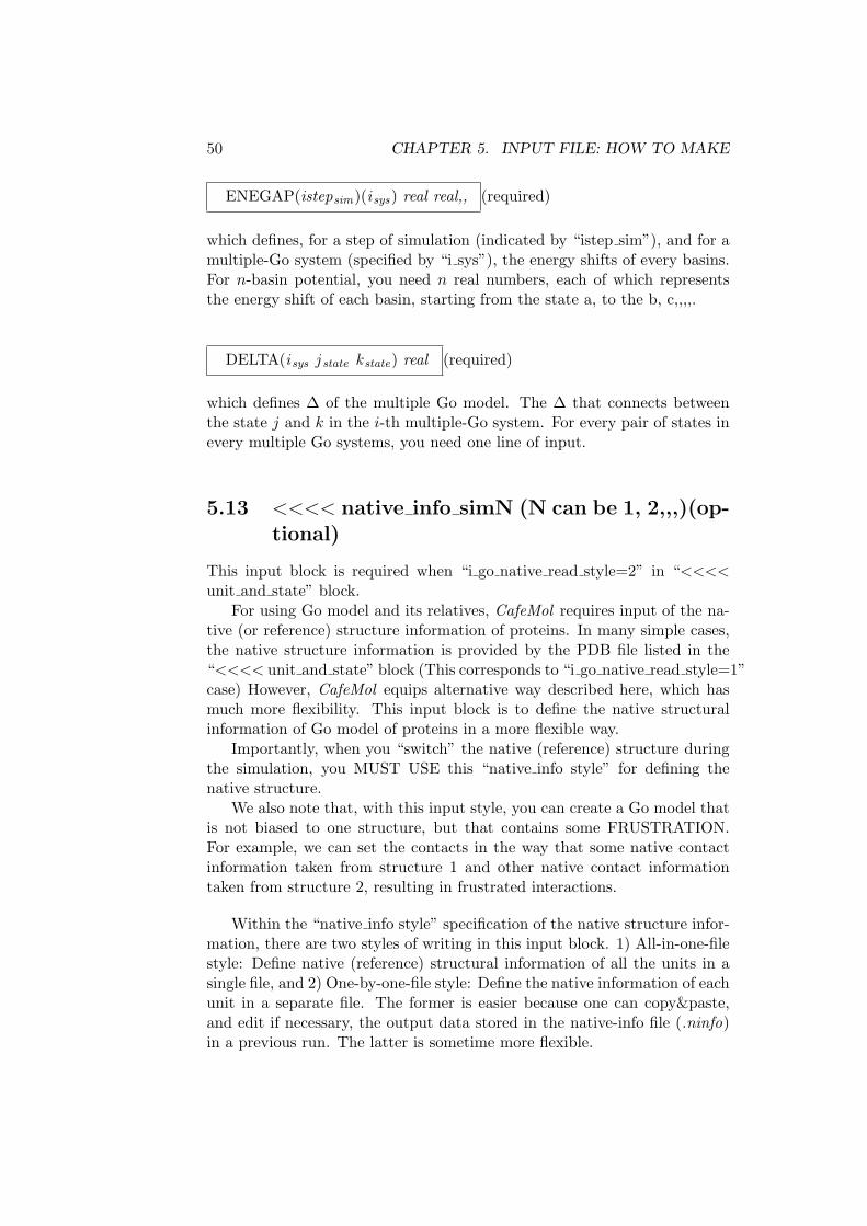
50 CHAPTER 5. INPUT FILE: HOW TO MAKE
ENEGAP(istepsim)(i sys) real real,, (required)
which defines, for a step of simulation (indicated by “istep sim”), and for amultiple-Go system (specified by “i sys”), the energy shifts of every basins.For n-basin potential, you need n real numbers, each of which representsthe energy shift of each basin, starting from the state a, to the b, c,,,,.
DELTA(i sys j state k state) real (required)
which defines ∆ of the multiple Go model. The ∆ that connects betweenthe state j and k in the i-th multiple-Go system. For every pair of states inevery multiple Go systems, you need one line of input.
5.13 <<<< native info simN (N can be 1, 2,,,)(op-tional)
This input block is required when “i go native read style=2” in “<<<<unit and state” block.
For using Go model and its relatives, CafeMol requires input of the na-tive (or reference) structure information of proteins. In many simple cases,the native structure information is provided by the PDB file listed in the“<<<< unit and state” block (This corresponds to “i go native read style=1”case) However, CafeMol equips alternative way described here, which hasmuch more flexibility. This input block is to define the native structuralinformation of Go model of proteins in a more flexible way.
Importantly, when you “switch” the native (reference) structure duringthe simulation, you MUST USE this “native info style” for defining thenative structure.
We also note that, with this input style, you can create a Go model thatis not biased to one structure, but that contains some FRUSTRATION.For example, we can set the contacts in the way that some native contactinformation taken from structure 1 and other native contact informationtaken from structure 2, resulting in frustrated interactions.
Within the “native info style” specification of the native structure infor-mation, there are two styles of writing in this input block. 1) All-in-one-filestyle: Define native (reference) structural information of all the units in asingle file, and 2) One-by-one-file style: Define the native information of eachunit in a separate file. The former is easier because one can copy&paste,and edit if necessary, the output data stored in the native-info file (.ninfo)in a previous run. The latter is sometime more flexible.

5.14. <<<< REDEFINE PARA (OPTIONAL) 51
The format for the native-info file is described in the Chapter 4. Weremark that the usage of the data is slightly, but importantly, differentbetween the two styles.
5.13.1 All-in-one-file style
By this, native structural information of all the units are given in a file. Inthe input file, all you need is to define the filename of it.
NINFO(all/ all) filename
where filename specifies the file name that contains all the native structuralinformation.
In this scheme, the columns of (absolute) sequential numbers of mp’s(imp1, imp2,,,,) in the native-info file are read (See Chapter 4).
5.13.2 One-by-one-file style
In this scheme, contents of the block are made of two types of lines. Thefirst is
NINFO(u&s1/u&s2 ) integer
which states that native structural information of the interaction betweenthe unit&state u&s1 and the unit&state u&s2 is defined in a file identifiedwith an integer. For systems with many units, many lines of this type are tobe written. These particular integer numbers are then linked to particularfiles in the second type of lines as
integer = filename
where the integer here should be equal to the integer found in lines of thefirst type. The filename is the name of the file that contains native structuralinformation.
We note that, in this scheme, the columns of sequential numbers of mpin each unit (e.g., imp1un, imp2un,,) in the native-info file are read. Thisstyle would be very useful to dynamically permutate the native-structuralinformation in the simulated complex, such as the case of F1-ATPase.
5.14 <<<< redefine para (optional)
This input block is required only when “i redef para=1” in “<<<< md information”block. Here, variety of input parameters can be modified from their default
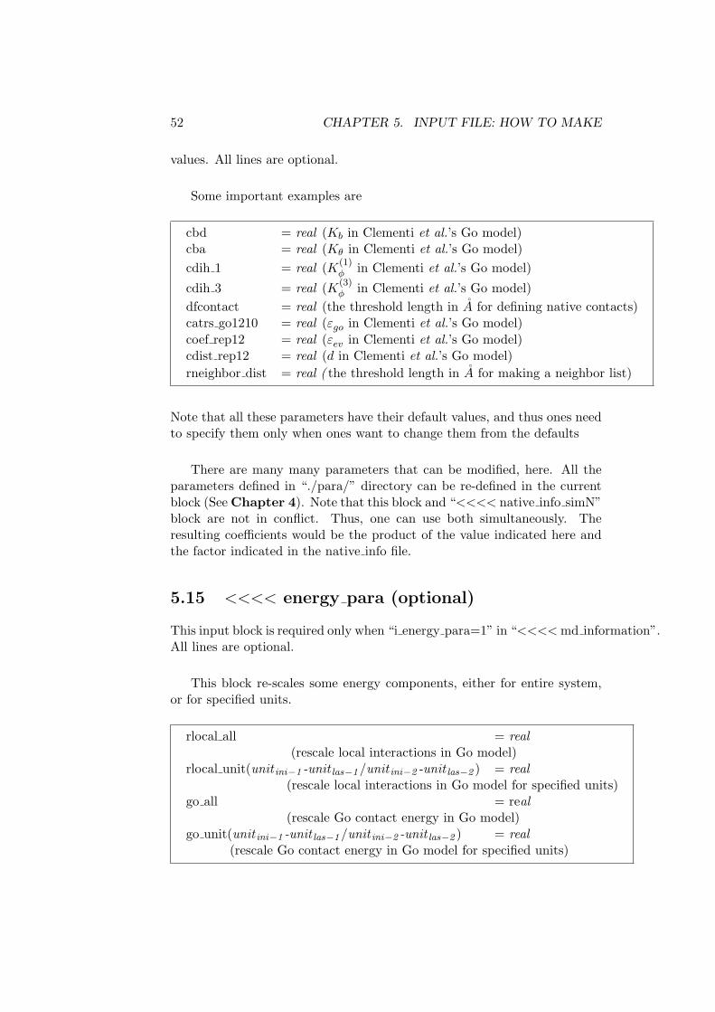
52 CHAPTER 5. INPUT FILE: HOW TO MAKE
values. All lines are optional.
Some important examples are
cbd = real (Kb in Clementi et al.’s Go model)cba = real (Kθ in Clementi et al.’s Go model)
cdih 1 = real (K(1)φ in Clementi et al.’s Go model)
cdih 3 = real (K(3)φ in Clementi et al.’s Go model)
dfcontact = real (the threshold length in A for defining native contacts)catrs go1210 = real (εgo in Clementi et al.’s Go model)
coef rep12 = real (εev in Clementi et al.’s Go model)cdist rep12 = real (d in Clementi et al.’s Go model)
rneighbor dist = real ( the threshold length in A for making a neighbor list)
Note that all these parameters have their default values, and thus ones needto specify them only when ones want to change them from the defaults
There are many many parameters that can be modified, here. All theparameters defined in “./para/” directory can be re-defined in the currentblock (See Chapter 4). Note that this block and “<<<< native info simN”block are not in conflict. Thus, one can use both simultaneously. Theresulting coefficients would be the product of the value indicated here andthe factor indicated in the native info file.
5.15 <<<< energy para (optional)
This input block is required only when “i energy para=1” in “<<<< md information”.All lines are optional.
This block re-scales some energy components, either for entire system,or for specified units.
rlocal all = real(rescale local interactions in Go model)
rlocal unit(unit ini−1 -unit las−1/unit ini−2 -unit las−2 ) = real(rescale local interactions in Go model for specified units)
go all = real(rescale Go contact energy in Go model)
go unit(unit ini−1 -unit las−1/unit ini−2 -unit las−2 ) = real(rescale Go contact energy in Go model for specified units)
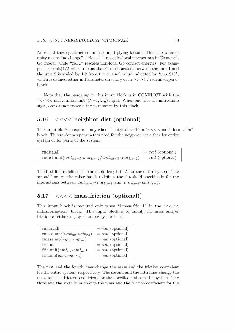
5.16. <<<< NEIGHBOR DIST (OPTIONAL) 53
Note that these parameters indicate multiplying factors. Thus the value ofunity means “no change”. “rlocal ,,” re-scales local interactions in Clementi’sGo model, while “go ,,,” rescales non-local Go contact energies. For exam-ple, “go unit(1/2)=1.2” means that Go interactions between the unit 1 andthe unit 2 is scaled by 1.2 from the original value indicated by “cgo1210”,which is defined either in Parameter directory or in “<<<< redefined para”block.
Note that the re-scaling in this input block is in CONFLICT with the“<<<< native info simN”(N=1, 2,,,) input. When one uses the native infostyle, one cannot re-scale the parameter by this block.
5.16 <<<< neighbor dist (optional)
This input block is required only when “i neigh dist=1” in “<<<< md information”block. This re-defines parameters used for the neighbor list either for entiresystem or for parts of the system.
rndist all = real (optional)rndist unit(unit ini−1 -unit las−1/unit ini−2 -unit las−2 ) = real (optional)
The first line redefines the threshold length in A for the entire system. Thesecond line, on the other hand, redefines the threshold specifically for theinteractions between unit ini−1 -unit las−1 and unit ini−2 -unit las−2 .
5.17 <<<< mass friction (optional)]
This input block is required only when “i mass fric=1” in the “<<<<md information” block. This input block is to modify the mass and/orfriction of either all, by chain, or by particles.
rmass all = real (optional)rmass unit(unit ini -unit las) = real (optional)rmass mp(mpini -mp las) = real (optional)fric all = real (optional)fric unit(unit ini -unit las) = real (optional)fric mp(mpini -mp las) = real (optional)
The first and the fourth lines change the mass and the friction coefficientfor the entire system, respectively. The second and the fifth lines change themass and the friction coefficient for the specified units in the system. Thethird and the sixth lines change the mass and the friction coefficient for the
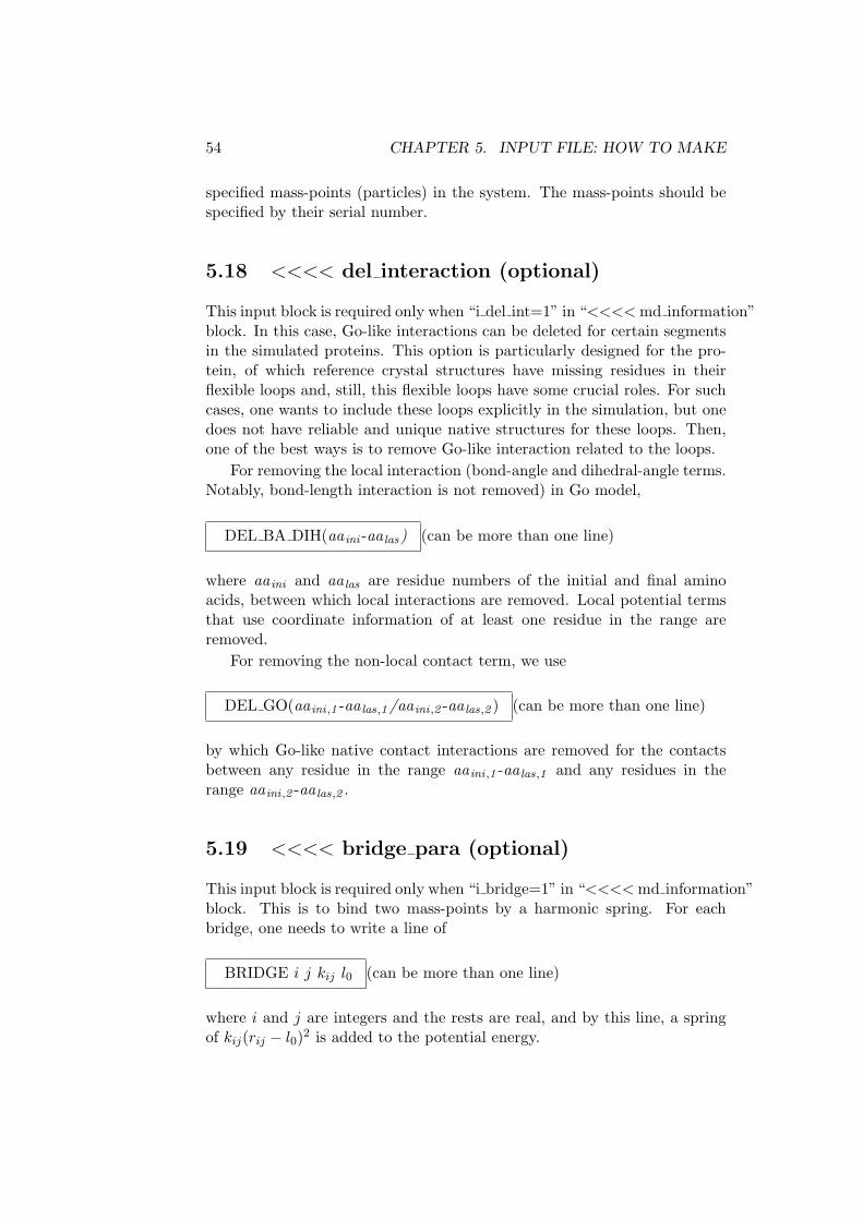
54 CHAPTER 5. INPUT FILE: HOW TO MAKE
specified mass-points (particles) in the system. The mass-points should bespecified by their serial number.
5.18 <<<< del interaction (optional)
This input block is required only when “i del int=1” in “<<<< md information”block. In this case, Go-like interactions can be deleted for certain segmentsin the simulated proteins. This option is particularly designed for the pro-tein, of which reference crystal structures have missing residues in theirflexible loops and, still, this flexible loops have some crucial roles. For suchcases, one wants to include these loops explicitly in the simulation, but onedoes not have reliable and unique native structures for these loops. Then,one of the best ways is to remove Go-like interaction related to the loops.
For removing the local interaction (bond-angle and dihedral-angle terms.Notably, bond-length interaction is not removed) in Go model,
DEL BA DIH(aa ini -aa las) (can be more than one line)
where aa ini and aa las are residue numbers of the initial and final aminoacids, between which local interactions are removed. Local potential termsthat use coordinate information of at least one residue in the range areremoved.
For removing the non-local contact term, we use
DEL GO(aa ini ,1 -aa las,1/aa ini ,2 -aa las,2 ) (can be more than one line)
by which Go-like native contact interactions are removed for the contactsbetween any residue in the range aa ini ,1 -aa las,1 and any residues in therange aa ini ,2 -aa las,2 .
5.19 <<<< bridge para (optional)
This input block is required only when “i bridge=1” in “<<<< md information”block. This is to bind two mass-points by a harmonic spring. For eachbridge, one needs to write a line of
BRIDGE i j kij l0 (can be more than one line)
where i and j are integers and the rests are real, and by this line, a springof kij(rij − l0)
2 is added to the potential energy.
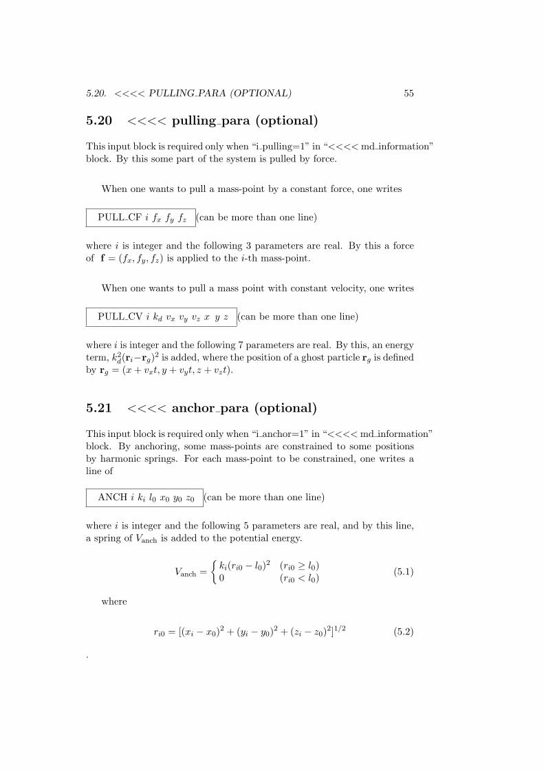
5.20. <<<< PULLING PARA (OPTIONAL) 55
5.20 <<<< pulling para (optional)
This input block is required only when “i pulling=1” in “<<<< md information”block. By this some part of the system is pulled by force.
When one wants to pull a mass-point by a constant force, one writes
PULL CF i fx fy fz (can be more than one line)
where i is integer and the following 3 parameters are real. By this a forceof f = (fx, fy, fz) is applied to the i-th mass-point.
When one wants to pull a mass point with constant velocity, one writes
PULL CV i kd vx vy vz x y z (can be more than one line)
where i is integer and the following 7 parameters are real. By this, an energyterm, k2
d(ri−rg)2 is added, where the position of a ghost particle rg is defined
by rg = (x + vxt, y + vyt, z + vzt).
5.21 <<<< anchor para (optional)
This input block is required only when “i anchor=1” in “<<<< md information”block. By anchoring, some mass-points are constrained to some positionsby harmonic springs. For each mass-point to be constrained, one writes aline of
ANCH i ki l0 x0 y0 z0 (can be more than one line)
where i is integer and the following 5 parameters are real, and by this line,a spring of Vanch is added to the potential energy.
Vanch =
{
ki(ri0 − l0)2 (ri0 ≥ l0)
0 (ri0 < l0)(5.1)
where
ri0 = [(xi − x0)2 + (yi − y0)
2 + (zi − z0)2]1/2 (5.2)
.
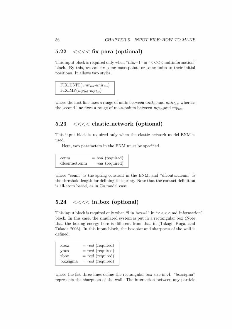
56 CHAPTER 5. INPUT FILE: HOW TO MAKE
5.22 <<<< fix para (optional)
This input block is required only when “i fix=1” in “<<<< md information”block. By this, we can fix some mass-points or some units to their initialpositions. It allows two styles,
FIX UNIT(unit ini -unit las)FIX MP(mpini -mp las)
where the first line fixes a range of units between unitiniand unitlas, whereasthe second line fixes a range of mass-points between mpiniand mplas.
5.23 <<<< elastic network (optional)
This input block is required only when the elastic network model ENM isused.
Here, two parameters in the ENM must be specified.
cenm = real (required)dfcontact enm = real (required)
where “cenm” is the spring constant in the ENM, and “dfcontact enm” isthe threshold length for defining the spring. Note that the contact definitionis all-atom based, as in Go model case.
5.24 <<<< in box (optional)
This input block is required only when “i in box=1” in “<<<< md information”block. In this case, the simulated system is put in a rectangular box (Notethat the boxing energy here is different from that in (Takagi, Koga, andTakada 2003). In this input block, the box size and sharpness of the wall isdefined.
xbox = real (required)ybox = real (required)zbox = real (required)boxsigma = real (required)
where the fist three lines define the rectangular box size in A. “boxsigma”represents the sharpness of the wall. The interaction between any particle

5.24. <<<< IN BOX (OPTIONAL) 57
with the wall is defined as
Vbox =
0 (d > 3σ)
Kbox
(
σd
)12(0.5σ < d < 3σ)
Kbox
(
σ0.5σ
)12 (1 + 120.5σ−d
0.5σ
)
(d < 0.5σ)
(5.3)
where d is the distance between the particle and the wall, σ represents thesharpness of the wall, “boxsigma”, Kbox is a large value (=10).

58 CHAPTER 5. INPUT FILE: HOW TO MAKE

Chapter 6
Examples: Input and output
Here, several examples of CafeMol runs are described. Comments and ex-planations for input format are included in ./inp/gbp mgo.inp.
6.1 Protein native dynamics and (un)folding withGo model at constant T
The first example is constant-temperature MD of a protein, SH3 domain,with the Go model. The example file is, as it is, to perform constant temper-ature (300K) Langevin MD of SH3 domain, a small β-sheet protein domainstarting from the native structure with pdb id=1srl.
6.1.1 Input & Output
The prepared input file is ./inp/sh3.inp, and PDB file for initial structureis ./pdb/1SRL.pdb. Just by changing the initial state to “i initial state=1”,one can simulate folding from a random conformation. Instead, if one re-places the temperature with “tempK=500”, say, one would observe quickunfolding.
The output files are given in ./data/sh3.*, where * corresponds to“data”, “ninfo”, and “ts”.
6.2 Automatic TF search
This example is to look for the folding transition temperature, TF at whichthe simulated protein reside in the native state for about half of the timeand is unfolded for the rest of time. The target protein is still SH3 domain.
59

60 CHAPTER 6. EXAMPLES: INPUT AND OUTPUT
6.2.1 Input & Output
The prepared input file is ./inp/sh3 stf.inp, and PDB file for initial struc-ture is ./pdb/1SRL.pdb.
The output files are given in ./data/sh3 stf.*, where * corresponds to“data”, “ninfo”, and “ts”.
6.3 Conformational transition simulation with mul-tiple basin model at constant temperature
This example conducts reversible closing and opening conformational changesof glutamine-binding protein with the multiple-basin potential.
6.3.1 Input & Output
The prepared input file is ./inp/gbp mgo1.inp, and PDB file for initialstructure is ./pdb/1WDN 2b.pdb. PDB files for reference structures are./pdb/1GGG 2.pdb and ./pdb/1WDN 2.pdb corresponding to open and closedstates, respectively.
The output files are given in ./data/gbp mgo1.*, where * correspondsto “data”, “ninfo”, and “ts”.
6.4 Cyclic conformational change simulation by switch-ing Go model at constant temperature
This is a simple example that employs “switching-Go” model. For the targetprotein of glutamine-binding protein, one starts the simulation using the Gomodel with the reference of the open conformation. At a certain time ofsimulation, one switches the reference structure into the closed one, whichpromptly induces large-scale conformation change of the protein.
Here, for switching, one uses the “native info” file as one of the inputdata. For this purpose, “all-in-one-file” style is more convenient and is usedin the example.
6.4.1 Input & Output
The prepared input file is ./inp/cafemol sw 1chain.inp, and PDB file forinitial structure is ./pdb/1GGG 2.pdb. As aforestated, while PDB file is notused for reference structure, ./ninfo/gbp1.ninfo and ./ninfo/gbp2.ninfo
are used.The output files are given in ./data/cafemool sw 1chain.*, where *
corresponds to “data”, “ninfo”, and “ts”.

6.5. ROTARY MOTION OF F1-ATPASE BY SWITCHING GO MODEL AT CONSTANT TEMPERATURE
6.5 Rotary motion of F1-ATPase by switching Gomodel at constant temperature
This is an example for simulation of rotary motion of F1-ATPase (We notethat the simulation scheme here is similar to, but not identical to, that in(Koga and Takada 2006)). It uses a minimal catalytic set, α3β3γ of whichX-ray structure of Walker (pdb id=1bmf.pdf) is used as the reference. Inthe crystal structure, chain pairs CD, AE, and BF are three pairs of αβ-subunits, in which the nucleotide-states are different each other; β-subunit ofchain D binds ADP, β-subunit of chain E is nucleotide-free (called empty),and β-subunit of chain F binds ATP-analog. Starting from this complexstructure, one switches the reference structures of the three αβ pairs so thatit drives chain CD into nucleotide-free state, chain AE into ATP-boundstate, and chain BF into ADP-bound state. After switching the potential,conformations of the α3β3 change, which is followed by the rotation of thecentral stalk γ that corresponds to chain G.
For this case, reference structures of the αβ-pair is permutated. Torealize it, the so-called “one-by-one-file” style “native info” files are utilized.
6.5.1 Input & Output
The prepared input file is ./inp/f1atp sw L onebyone.inp, and PDB filesfor initial structure are ./pdb/gamma.pdb and ./pdb/# *.pdb where # cor-responds to “alpha” and “beta”, and * corresponds to “E” and “TP”, and“DP”. The “native info” files are given in ./ninfo/f1atp *.ninfo, where *
corresponds to “alpha E”, “alpha TP”, “alpha DP”, “beta E”, “beta TP”,“beta DP”, “gamma”, “alphE betaE”, “alphE betaDP”, “alphTP betaE”,“alphTP betaTP”, “alphDP betaTP”, and “alphDP betaDP”.
The output files are given in ./data/f1atp sw L onebyone.*, where *
corresponds to “data”, “ninfo”, and “ts”.

62 CHAPTER 6. EXAMPLES: INPUT AND OUTPUT
Bibliography
Berendsen, H., J. Postma, W. Van Gunsteren, A. DiNola, and
J. Haak (1984): “Molecular dynamics with coupling to an external bath,”The Journal of Chemical Physics, 81, 3684.
Brooks, B., R. Bruccoleri, B. Olafson, D. States, S. Swami-
nathan, and M. Karplus (1983): “CHARMM: A program for macro-molecular energy, minimization, and dynamics calculations Supported inpart by grants from the National Science Foundation and the NationalInstitutes of Health.,” Journal of Computational Chemistry, 4(2).
Bryngelson, J., and P. Wolynes (1987): “Spin glasses and the statisticalmechanics of protein folding,” Proceedings of the National Academy ofSciences, 84(21), 7524–7528.
Clementi, C., H. Nymeyer, and J. Onuchic (2000): “Topological andenergetic factors: what determines the structural details of the transi-tion state ensemble and gen-routeh intermediates for protein folding? Aninvestigation for small globular proteins,” Journal of Molecular Biology,298(5), 937–953.
Go, N. (1983): “Theoretical studies of protein folding,” Annual review ofbiophysics and bioengineering, 12(1), 183–210.
Guo, Z., and D. Thirumalai (1995): “Kinetics of protein folding: nucle-ation mechanism, time scales, and pathways,” Biopolymers, 36(1).
Honeycutt, J., and D. Thirumalai (1992): “The nature of folded statesof globular proteins,” Biopolymers, 32(6).
Humphrey, W., A. Dalke, and K. Schulten (1996): “VMD: visualmolecular dynamics,” Journal of Molecular Graphics, 14(1), 33–38.
Koga, N., and S. Takada (2001): “Roles of native topology and chain-length scaling in protein folding: a simulation study with a Go-likemodel,” Journal of Molecular Biology, 313(1), 171–180.
63
64 BIBLIOGRAPHY
(2006): “Folding-based molecular simulations reveal mechanismsof the rotary motor F1–ATPase,” Proceedings of the National Academyof Sciences, 103(14), 5367.
Leopold, P., M. Montal, and J. Onuchic (1992): “Protein foldingfunnels: a kinetic approach to the sequence-structure relationship,” Pro-ceedings of the National Academy of Sciences, 89(18), 8721–8725.
Okazaki, K., N. Koga, S. Takada, J. Onuchic, and P. Wolynes
(2006): “Multiple-basin energy landscapes for large-amplitude conforma-tional motions of proteins: Structure-based molecular dynamics simula-tions,” Proceedings of the National Academy of Sciences, 103(32), 11844.
Phillips, J., R. Braun, W. Wang, J. Gumbart, E. Tajkhorshid,
E. Villa, C. Chipot, R. Skeel, L. Kale, and K. Schulten (2005):“Scalable molecular dynamics with NAMD,” Journal of ComputationalChemistry, 26(16), 1781.
Smit, B., and D. Frenkel (2006): Understanding molecular simulation:From algorithms to applications. Academic Press.
Takagi, F., N. Koga, and S. Takada (2003): “How protein thermo-dynamics and folding mechanisms are altered by the chaperonin cage:Molecular simulations,” Proceedings of the National Academy of Sciences,100(20), 11367–11372.
Tirion, M. (1996): “Large amplitude elastic motions in proteins from asingle-parameter, atomic analysis,” Physical Review Letters, 77(9), 1905–1908.


![Baritone (5tü) OJI] Piano Masanori Kato Naoto …Baritone (5tü) OJI] Piano Masanori Kato Naoto Sakiya, Violin Satoru Sakurada, Violin Kyoko Takano, Viola Hiroki Kadowaki, Cello ,9/22](https://img.pdfslide.tips/doc/110x75/5e697f7be7d31d7e267b19e4/baritone-5t-oji-piano-masanori-kato-naoto-baritone-5t-oji-piano-masanori.jpg)