Embed Size (px)
Citation preview
無線通信システム特論第 2回 無線通信路の基礎Advanced Radio Communication Systems2nd Class: Basics of Radio Propagation
Koichi AdachiApril 15, 2018
Advanced Wireless & Communication Research Center (AWCC)The University of Electro-Communications (UEC), JapanSlides available@ http://www.awcc.uec.ac.jp/adachilab/lecture/adv_commun

Basics of Radio Propagation

Course Outline and Weekly Schedule
1. (8/4) Introduction of Wireless Communications Systems2. (15/4) Basics of Radio Propagation ð Today3. (22/4) Probability and Fourier Transform4. (6/5) Matched Filter and Correlation Receiver5. (13/5) Maximum Likelihood Estimation6. (20/5) Antipodal Signaling7. (27/5) Basics of Modulation8. (3/6) Basics of Demodulation9. (10/6) Spread Spectrum
10. (17/6) Theory of Diversity11. (24/6) OFDM12. (1/7) Multi Antenna Transmission I13. (8/7) Multi Antenna Transmission II14. (22/7) Multiple Access Protocol15. (29/7) State of The Art Technology
Copyright ©K. Adachi, AWCC, UEC, 2018 2 / 47
Wireless Propagation Channel
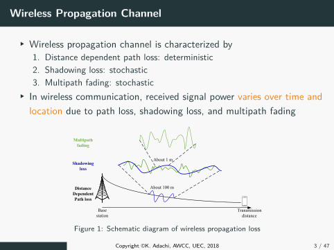
§ Wireless propagation channel is characterized by1. Distance dependent path loss: deterministic2. Shadowing loss: stochastic3. Multipath fading: stochastic
§ In wireless communication, received signal power varies over time andlocation due to path loss, shadowing loss, and multipath fading
Transmission
distance
Base
station
Distance
Dependent
Path loss
Shadowing
loss
Multipath
fading
About 100 m
About 1 m
Figure 1: Schematic diagram of wireless propagation loss
Copyright ©K. Adachi, AWCC, UEC, 2018 3 / 47
Wireless Propagation Channel
§ Path loss depends on the physical distance from a transmission pointto a reception point
§ Shadowing loss varies irregularly in the interval of from a few tens ofmeters to a few hundreds of meters
§ Multipath fading varies irregularly in the interval of about a half ofwavelength of a carrier frequency
Copyright ©K. Adachi, AWCC, UEC, 2018 4 / 47

Path loss
§ Line-of-sight (LoS) propagation environment:§ There is a direct radio wave propagation path from a transmitter to a
receiver§ Non line-of-sight (NLoS) propagation environment:
§ Due to the obstacles, there is no direct propagation path from atransmitter to a receiver
LoS environment
NLoS environment
Figure 2: LoS & NLoS environment.
Copyright ©K. Adachi, AWCC, UEC, 2018 5 / 47
Free Space Propagation
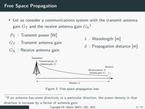
§ Let us consider a communications system with the transmit antennagain GT and the receive antenna gain GR
1
PT : Transmit power [W]GT : Transmit antenna gainGR : Receive antenna gain
λ : Wavelength [m]d : Propagation distance [m]
Receiver
Transmitter
Transmit power: Pt
Antenna gain: Gt
Receive power: Pr
Antenna gain: Gr
Distance: d
Figure 3: Free space propagation loss.
1If an antenna has some directivity in a particular direction, the power density in thatdirection is increase by a factor of antenna gain.
Copyright ©K. Adachi, AWCC, UEC, 2018 6 / 47
Free Space Propagation
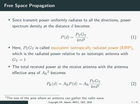
§ Since transmit power uniformly radiates to all the directions, powerspectrum density at the distance d becomes
P pdq “PTGT4πd2 . (1)
§ Here, PTGT is called equivalent isotropically radiated power (EIRP),which is the radiated power relative to an isotoropic antenna withGT “ 1
§ The total received power at the receive antenna with the antennaeffective area of AR
2 becomes
PRpdq “ ARP pdq “ ARPTGT4πd2 . (2)
2The size of the area where an antenna can gather the radio waveCopyright ©K. Adachi, AWCC, UEC, 2018 7 / 47

Antenna Effective Area
§ The antenna effective area AR is related the antenna gain GR asfollows:
ArR “λ2
4πGR. (3)
§ Thus, in a free space, received power is expressed as follows:
Friis transmission equation & Free-Space Propagation Loss
PRpdq “1
LppdqPTGTGR, (4a)
Lppdq “
ˆ
4πd
λ
˙2. (4b)
Copyright ©K. Adachi, AWCC, UEC, 2018 8 / 47
Received Power in dB Domain
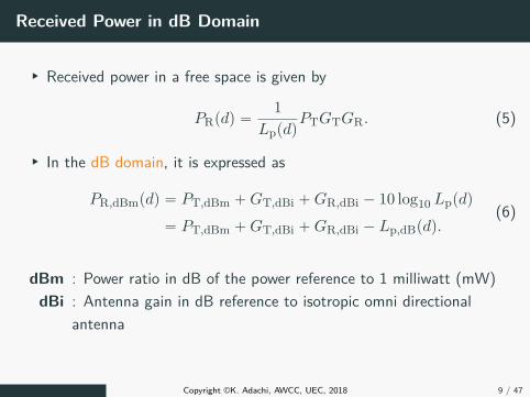
§ Received power in a free space is given by
PRpdq “1
LppdqPTGTGR. (5)
§ In the dB domain, it is expressed as
PR,dBmpdq “ PT,dBm ` GT,dBi ` GR,dBi ´ 10 log10 Lppdq
“ PT,dBm ` GT,dBi ` GR,dBi ´ Lp,dBpdq.(6)
dBm : Power ratio in dB of the power reference to 1 milliwatt (mW)dBi : Antenna gain in dB reference to isotropic omni directional
antenna
Copyright ©K. Adachi, AWCC, UEC, 2018 9 / 47
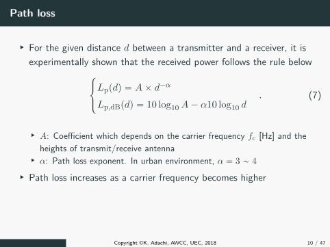
Path loss
§ For the given distance d between a transmitter and a receiver, it isexperimentally shown that the received power follows the rule below
$
&
%
Lppdq “ A ˆ d´α
Lp,dBpdq “ 10 log10 A ´ α10 log10 d. (7)
§ A: Coefficient which depends on the carrier frequency fc [Hz] and theheights of transmit/receive antenna
§ α: Path loss exponent. In urban environment, α “ 3 „ 4
§ Path loss increases as a carrier frequency becomes higher
Copyright ©K. Adachi, AWCC, UEC, 2018 10 / 47
Path Loss Exponent
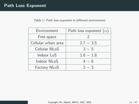
Table 1: Path loss exponent in different environment
Environment Path loss exponent (α)Free space 2
Cellular urban area 2.7 „ 3.5Cellular NLoS 3 „ 5
Indoor LoS 1.6 „ 1.8Indoor NLoS 4 „ 6Factory NLoS 2 „ 3
Copyright ©K. Adachi, AWCC, UEC, 2018 11 / 47
Practical Path Loss Model
§ However, in the practical scenario, there are a number of obstaclessuch as buildings between a transmitter and a receiver
§ Many monographs are obtained through propagation measurements§ Okumura-Hata model3 is one of the most famous path loss models that
are obtained from propagation measurements
3This name indicates Hata model which is an empirical formulation based on the dataset from Okumura model
Copyright ©K. Adachi, AWCC, UEC, 2018 12 / 47

Okumura-Hata Model i
§ Urban area4:
LPU,dBpdq “ 69.55 ` 26.16 ¨ log fc ´ 13.82 ¨ log hb ´ aphmq
` p44.9 ´ 6.55 ¨ log hbq ¨ log d. (8)
aphmq : Correction factor for antenna height of MT§ Small- and medium-size city:
aphmq “ p1.1 ¨ log fc ´ 0.7qhm ´ p1.56 ¨ log fc ´ 0.8q. (9)
Copyright ©K. Adachi, AWCC, UEC, 2018 13 / 47

Okumura-Hata Model ii
§ Large city:
aphmq “
#
8.29 ¨ plogp1.54 ¨ hmqq2 ´ 1.1 for 150 ď fc ď 200 rMHzs
3.2 ¨ plogp11.75 ¨ hmqq2 ´ 4.97 for 400 ď fc rMHzs ď 1500.
(10)
§ Suburban area:
LPS,dBpdq “ LPU,dBpdq ´ 2 ¨ plogpfc28qq2
´ 5.4. (11)
§ Open area:
LPO,dBpdq “ LPU,dBpdq ´ 4.78 ¨ plog fcq2
` 18.33 ¨ log fc ´ 40.94.
(12)
§ Parameters:
Copyright ©K. Adachi, AWCC, UEC, 2018 14 / 47

Okumura-Hata Model iii
fc : Carrier frequency [MHz] (150„1500 [MHz])hb : Effective height of BS antenna [m] (30„200 [m])hm : Height of MT antenna [m] (1„10 [m])
d : Distance [km] (1„20 [km])
Copyright ©K. Adachi, AWCC, UEC, 2018 15 / 47
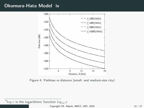
Okumura-Hata Model iv
−170
−160
−150
−140
−130
−120
−110
−100
4 8 12 16 20
fc=200 [MHz]
fc=400 [MHz]
fc=800 [MHz]
fc=1500 [MHz]
Pat
h l
oss
[dB
]
Distance, R [km]
Figure 4: Pathloss vs distance (small- and medium-size city)
4log x is the logarithmic function log10 xCopyright ©K. Adachi, AWCC, UEC, 2018 16 / 47

Shadowing
§ Radio waves radiated from a transmitter are blocked by obstacles suchas huge buildings ñ Shadowing
§ Temporal variation of shadowing is much slower compared to fastfading ñ The signal power over time is varying slowly
§ Due to shadowing, the average received power at the same distancesfrom a transmitter are different from each other
Copyright ©K. Adachi, AWCC, UEC, 2018 17 / 47

Shadowing i
§ It has been experimentally shown that the logarithm of the localaverage received power S follows the normal distribution with thestandard deviation of σ:
ppδq “1
?2πσ
exp
˜
´
`
δ ´ δ˘2
2σ2
¸
, (13)
where δ “ 10 log10 S
§ The distribution of S becomes
ppSq “10
ln 10¨
1?
2πσ2Sexp
ˆ
´p10 log10 S ´ Sq2
2σ2
˙
. (14)
Copyright ©K. Adachi, AWCC, UEC, 2018 18 / 47

Shadowing ii
0
0.05
0.1
0.15
0.2
-20 -15 -10 -5 0 5 10 15 20
p(η)
η
0
0.1
0.2
0.3
0.4
0.5
0.6
0.7
0.8
0 2 4 6 8 10
p(ξ)
ξ
2
2
1 ( )( ) exp
22g
η − µη = − σπσ
2
10
2
(10 log )10 1( ) exp
ln10 22f
ξ − µξ = ⋅ − σπσξ
1010ηξ =
Figure 5: Distribution of shadowing in log domain and real domain.
Copyright ©K. Adachi, AWCC, UEC, 2018 19 / 47
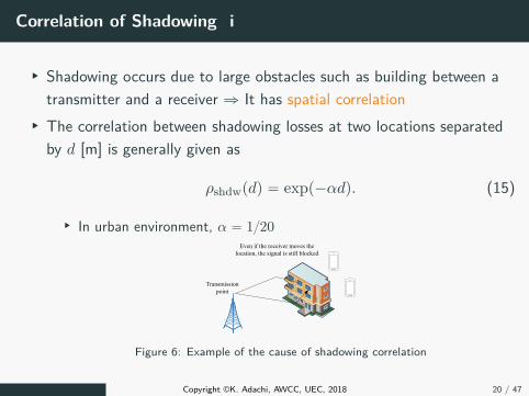
Correlation of Shadowing i
§ Shadowing occurs due to large obstacles such as building between atransmitter and a receiver ñ It has spatial correlation
§ The correlation between shadowing losses at two locations separatedby d [m] is generally given as
ρshdwpdq “ expp´αdq. (15)
§ In urban environment, α “ 120
Transmission
point
Even if the receiver moves the
location, the signal is still blocked
Figure 6: Example of the cause of shadowing correlation
Copyright ©K. Adachi, AWCC, UEC, 2018 20 / 47

Correlation of Shadowing ii
Figure 7: Example of correlated shadowing
Copyright ©K. Adachi, AWCC, UEC, 2018 21 / 47
Fast Fading
§ Radio waves reaching the surroundings of an MT are scattered(reflected and diffracted) by local scattererssñ These scattered radio waves form multiple propagation paths.
§ Received signal power varies significantly as an MT slightly movesbecause receiving condition from scatterers changes
Copyright ©K. Adachi, AWCC, UEC, 2018 22 / 47

Received Signal from View Point of Temporal Variation
§ Let’s consider the scenario when N plain waves created by the localscatterers are arriving at the receiving point
§ N plain waves are assumed to have the same amplitude but thedifferent phases
Point
(0,0)
Point
(x,y)
d x
y
Direction of arrival (DoA) of
nth plain wave, θn
Figure 8: The nth plain wave with direction of arrival (DoA) of θn
Copyright ©K. Adachi, AWCC, UEC, 2018 23 / 47

Fast Fading
§ The phase of the nth plain wave is advanced by ξnpx, yq relative tothe phase at p0, 0q
§ The phase difference ξnpx, yq is given by
ξnpx, yq “ 2πd
λ“ 2π
y cos θn ´ x sin θn
λ. (16)
§ The channel observed at the point px, yq is given by
hpx, yq “1
?N
N´1ÿ
n“0exp pj pξnpx, yq ` ϕnqq , (17)
where ϕn is the phase of the nth plain wave at the point px, yq
Copyright ©K. Adachi, AWCC, UEC, 2018 24 / 47

Received Signal from View Point of Temporal Variation
§ Let us consider the scenario when a receiver is moving along they-axis at the constant speed v [m/s]
38.7°θn
(0,0)
(x,y)=(0,vt)
d x
y
Moving at
v[m/s]
Figure 9: Doppler effect due to the movement of mobile terminal
Copyright ©K. Adachi, AWCC, UEC, 2018 25 / 47
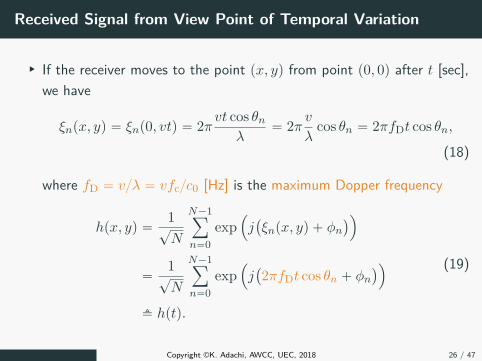
Received Signal from View Point of Temporal Variation
§ If the receiver moves to the point px, yq from point p0, 0q after t [sec],we have
ξnpx, yq “ ξnp0, vtq “ 2πvt cos θn
λ“ 2π
v
λcos θn “ 2πfDt cos θn,
(18)
where fD “ vλ “ vfcc0 [Hz] is the maximum Dopper frequency
hpx, yq “1
?N
N´1ÿ
n“0exp
´
j`
ξnpx, yq ` ϕn
˘
¯
“1
?N
N´1ÿ
n“0exp
´
j`
2πfDt cos θn ` ϕn
˘
¯
fi hptq.
(19)
Copyright ©K. Adachi, AWCC, UEC, 2018 26 / 47
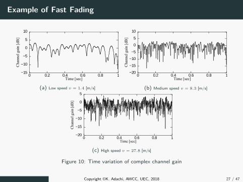
Example of Fast Fading
−15
−10
−5
0
5
10
0 0.2 0.4 0.6 0.8 1
Ch
ann
el g
ain
[d
B]
Time [sec]
(a) Low speed v “ 1.4 [m/s]
−20
−15
−10
−5
0
5
10
0 0.2 0.4 0.6 0.8 1
Ch
ann
el g
ain
[d
B]
Time [sec]
(b) Medium speed v “ 8.3 [m/s]
−20
−15
−10
−5
0
5
0 0.2 0.4 0.6 0.8 1
Ch
annel
gai
n [
dB
]
Time [sec]
(c) High speed v “ 27.8 [m/s]
Figure 10: Time variation of complex channel gain
Copyright ©K. Adachi, AWCC, UEC, 2018 27 / 47
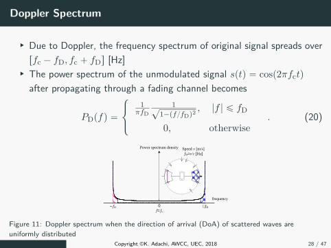
Doppler Spectrum
§ Due to Doppler, the frequency spectrum of original signal spreads overrfc ´ fD, fc ` fDs [Hz]
§ The power spectrum of the unmodulated signal sptq “ cosp2πfctq
after propagating through a fading channel becomes
PDpfq “
$
&
%
1πfD
1?1´pffDq2 , |f | ď fD
0, otherwise. (20)
0f=fc
+fD−fD
Speed v [m/s]
fD=v/c [Hz]Power spectrum density
frequency
Figure 11: Doppler spectrum when the direction of arrival (DoA) of scattered waves areuniformly distributed
Copyright ©K. Adachi, AWCC, UEC, 2018 28 / 47

Time Selective Fading
§ Due to Doppler, the amplitude of received signal fluctuates in timeñ Time selective fading
§ The time duration over which channel amplitude can be considered asconstant is called coherence time
§ The coherence time Tc and the maximum Doppler frequency fD havethe following relationship
Tc «1
fD. (21)
§ The 50% coherence time is given as
Tc “
d
916πf2
D»
0.423fD
. (22)
Copyright ©K. Adachi, AWCC, UEC, 2018 29 / 47

Channel Impulse Response
§ Reflectors existing between a transmitter and a receiver createsdifferent paths§ For example, if the propagation difference between the paths created by
multiple reflectors is 300 [m], the transmitted signal arrives at a receiverwith 1 µsec apart
§ If the time delay difference due to the reflectors is more than theinverse of the signal bandwidth W [Hz], multiple paths are created
Wireless
propagation
h(t)
Time Time delay
Am
pli
tude
Am
pli
tude
Each path is formed by a number of unresolvable paths
and is represented by one impulse hl(t)
t=0 t=0
Input impulse
τ0 τ1 τ2
Figure 12: Example of channel impulse response
Copyright ©K. Adachi, AWCC, UEC, 2018 30 / 47
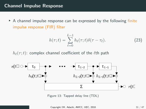
Channel Impulse Response
§ A channel impulse response can be expressed by the following finiteimpulse response (FIR) filter
hpτ ; tq “
L´1ÿ
ℓ“0hℓpτ ; tqδpτ ´ τℓq. (23)
hℓpτ ; tq: complex channel coefficient of the ℓth path
τ0 τL−1
h0(τ;t) hL−1(τ;t)hL−2(τ;t)
τL−2
Σ
s(t)
r(t)
Figure 13: Tapped delay line (TDL)
Copyright ©K. Adachi, AWCC, UEC, 2018 31 / 47
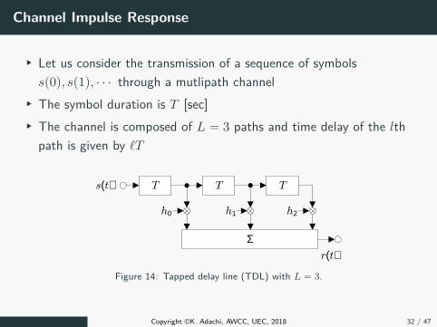
Channel Impulse Response
§ Let us consider the transmission of a sequence of symbolssp0q, sp1q, ¨ ¨ ¨ through a mutlipath channel
§ The symbol duration is T [sec]§ The channel is composed of L “ 3 paths and time delay of the lth
path is given by ℓT
T T
h0 h2h1
T
Σ
s(t)
r(t)
Figure 14: Tapped delay line (TDL) with L “ 3.
Copyright ©K. Adachi, AWCC, UEC, 2018 32 / 47

Channel Impulse Response
§ At time t “ 0, sp0q is transmitted§ At time t “ T , sp1q is transmitted and sp0q is received after
propagating the channel h0§ At time t “ 2T , sp2q is transmitted and sp0q and sp1q are received
after propagating the channel h1 and h0, respectively§ At time t “ 3T , sp3q is transmitted and sp0q, sp1q, and sp2q are
received after propagating the channel h2, h1, and h0, respectively
T T
h0 h2h1
T
Σ
s(3)
r(3T)=h2s(0)+h1s(1)+h0s(2)
s(2) s(1) s(0)
Figure 15: At time t “ 3T .
Copyright ©K. Adachi, AWCC, UEC, 2018 33 / 47

Channel Impulse Response
§ The received signal after propagating L resolvable paths is expressedas
rptq “ sptq b hpτ ; tq
“
ż 8
´8
spt ´ τqhpτ ; tqdτ
“
L´1ÿ
ℓ“0hℓptqspt ´ τℓq.
(24)
§ Please note that each path hℓptq is composed of unresolvable N plainwaves
Copyright ©K. Adachi, AWCC, UEC, 2018 34 / 47
Channel Impulse Response
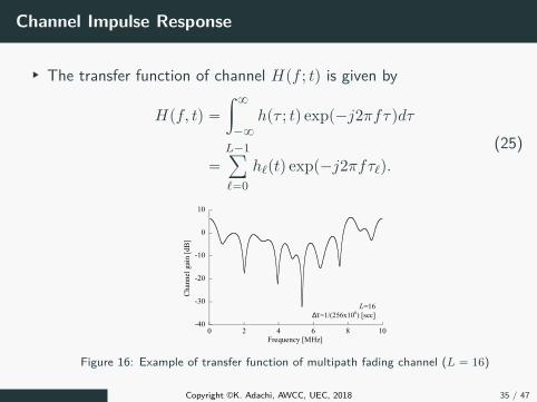
§ The transfer function of channel Hpf ; tq is given by
Hpf, tq “
ż 8
´8
hpτ ; tq expp´j2πfτqdτ
“
L´1ÿ
ℓ“0hℓptq expp´j2πfτℓq.
(25)
L=16
∆τ=1/(256x106) [sec]
-40
-30
-20
-10
0
10
0 2 4 6 8 10
Ch
ann
el g
ain
[d
B]
Frequency [MHz]
Figure 16: Example of transfer function of multipath fading channel (L “ 16)
Copyright ©K. Adachi, AWCC, UEC, 2018 35 / 47

Multipath Channel
§ If only one path exists, i.e., L “ 1, the transfer function is given by$
&
%
Hpf, tq “ h0ptq expp´j2πfτ0q
|Hpf, tq| “ |h0ptq|. (26)
ñ The transfer function Hpf, tq is constant over the frequency, i.e.,frequency non-selective channel
|H(f,t)|
f
|h0(t)|
Figure 17: Example of channel transfer function Hpf, tq when L “ 1
Copyright ©K. Adachi, AWCC, UEC, 2018 36 / 47

Multipath Channel
§ If there are two paths, i.e., L “ 2, the transfer function is given by$
’
&
’
%
Hpf, tq “ h0ptq expp´j2πfτ0q ` h1ptq expp´j2πfτ1q
|Hpf, tq| “ |h0 ptq| ˆ
ˇ
ˇ
ˇ
ˇ
1 `h1 ptq
h0 ptqexpp´j2πf∆τq
ˇ
ˇ
ˇ
ˇ
. (27)
ñ The transfer function Hpf, tq is a function of the frequency, i.e.,frequency selective channel
|H(f,t)|
f
∆f=1/∆τ1+|h1(t)/h0(t)|
1−|h1(t)/h0(t)|
If the difference between two paths
is ∆τ=1 [µsec], then ∆f=1 [MHz]
Figure 18: Example of channel transfer function Hpf, tq when L “ 2
Copyright ©K. Adachi, AWCC, UEC, 2018 37 / 47
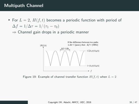
Multipath Channel
§ For L “ 2, Hpf, tq becomes a periodic function with period of∆f “ 1∆τ “ 1 pτ1 ´ τ0q
ñ Channel gain drops in a periodic manner
|H(f,t)|
f
∆f=1/∆τ1+|h1(t)/h0(t)|
1−|h1(t)/h0(t)|
If the difference between two paths
is ∆τ=1 [µsec], then ∆f=1 [MHz]
Figure 19: Example of channel transfer function Hpf, tq when L “ 2
Copyright ©K. Adachi, AWCC, UEC, 2018 38 / 47

Narrowband Channel and Broadband Channel
§ Narrowband channel§ Transfer function is almost constant within signal bandwidth§ All frequency components of the signal are affected by the same
amplitude and the phase change§ Broadband channel
§ Transfer function varies within signal bandwidth§ Different frequency components of signal are affected by the different
amplitude and the phase change
-15
-10
-5
0
5
0 2 4 6 8 10
| H(f
,t)|
[dB
]
Frequency f [MHz]
Broadband transmission
(Several MHz)
Narrowband transmission
(Several 10KHz)
Figure 20: Example of narrowband channel and broadband channelCopyright ©K. Adachi, AWCC, UEC, 2018 39 / 47

Power Delay Profile
§ Power delay profile represents how received signal power exists in thedelay time domain, which is defined as
Ωpτq fi E”
|hpτ ; tq|2ı
“
L´1ÿ
ℓ“0E
”
|hℓptq|2ı
δpτ ´ τℓq,
(28)
whereż 8
´8
Ωpτqdτ “ 1. (29)
Delay time τ
Ω(τ)
τ0 τ1 τ2 τL-1
Copyright ©K. Adachi, AWCC, UEC, 2018 40 / 47
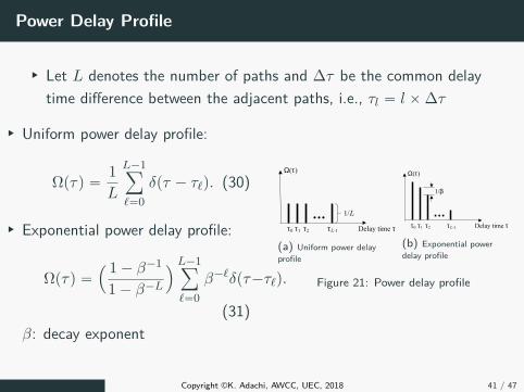
Power Delay Profile
§ Let L denotes the number of paths and ∆τ be the common delaytime difference between the adjacent paths, i.e., τl “ l ˆ ∆τ
§ Uniform power delay profile:
Ωpτq “1L
L´1ÿ
ℓ“0δpτ ´ τℓq. (30)
§ Exponential power delay profile:
Ωpτq “
´ 1 ´ β´1
1 ´ β´L
¯L´1ÿ
ℓ“0β´ℓδpτ´τℓq.
(31)β: decay exponent
Delay time τ
Ω(τ)
τ0 τ1 τ2 τL-1
1/L
(a) Uniform power delayprofile
Delay time ττ0 τ1 τ2 τL-1
1/β
Ω(τ)
(b) Exponential powerdelay profile
Figure 21: Power delay profile
Copyright ©K. Adachi, AWCC, UEC, 2018 41 / 47

Delay Spread
§ Delay spread5 indicates how much the channel spreads in time, whichis given by
τrms fi
d
ż 8
´8
Ωpτqpτ ´ τq2dτ, (32)
whereτ “
ż 8
´8
τΩpτqdτ. (33)
§ Delay spread is used to measure the channel frequency selectivity§ If the symbol duration (the inverse of the frequency bandwidth) is
much longer than the delay spread, the impact ofinter-symbol-interference (ISI) is negligible
5The most common metric for delay spread is root mean square (rms) delay spreadCopyright ©K. Adachi, AWCC, UEC, 2018 42 / 47
Coherence Bandwidth
§ The frequency bandwidth over which the channel transfer functioncan be considered as constant is called coherence bandwidth
§ The coherence bandwidth Wc and the delay spread τrms have thefollowing relationship
§ For frequency correlation above 0.9, the coherence bandwidth is approximately
Wc «1
50τrms. (34)
§ For frequency correlation above 0.5, the coherence bandwidth is approximately
Wc «1
5τrms. (35)
Copyright ©K. Adachi, AWCC, UEC, 2018 43 / 47
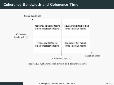
Coherence Bandwidth and Coherence Time
Frequency flat fading
Time nonselective fading
Frequency selective fading
Time nonselective fading
Frequency selective fading
Time selective fading
Frequency flat fading
Time selective fading
Signal bandwidth
Signal duration
Coherence time, Tc
Coherence
bandwidth, Wc
Figure 22: Coherence bandwidth and coherence time
Copyright ©K. Adachi, AWCC, UEC, 2018 44 / 47
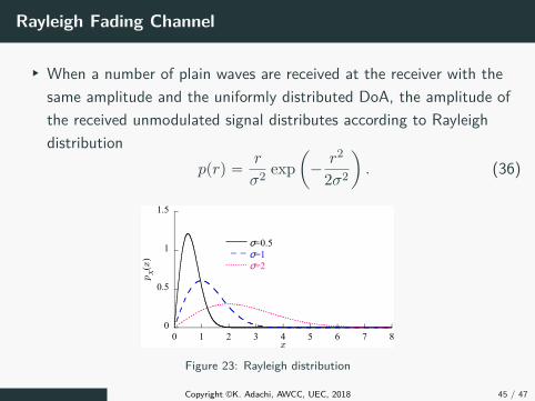
Rayleigh Fading Channel
§ When a number of plain waves are received at the receiver with thesame amplitude and the uniformly distributed DoA, the amplitude ofthe received unmodulated signal distributes according to Rayleighdistribution
pprq “r
σ2 expˆ
´r2
2σ2
˙
. (36)
0
0.5
1
1.5
0 1 2 3 4 5 6 7 8
σ=0.5σ=1σ=2
pX(x)
x
Figure 23: Rayleigh distribution
Copyright ©K. Adachi, AWCC, UEC, 2018 45 / 47
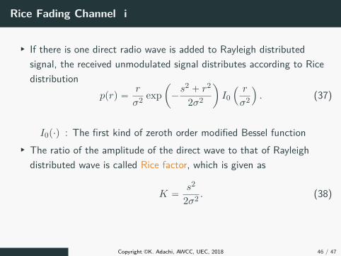
Rice Fading Channel i
§ If there is one direct radio wave is added to Rayleigh distributedsignal, the received unmodulated signal distributes according to Ricedistribution
pprq “r
σ2 expˆ
´s2 ` r2
2σ2
˙
I0
´ r
σ2
¯
. (37)
I0p¨q : The first kind of zeroth order modified Bessel function§ The ratio of the amplitude of the direct wave to that of Rayleigh
distributed wave is called Rice factor, which is given as
K “s2
2σ2 . (38)
Copyright ©K. Adachi, AWCC, UEC, 2018 46 / 47

Rice Fading Channel ii
0
0.2
0.4
0.6
0.8
1
0 2 4 6 8
K=0K=1K=10
pX(x)
x
Figure 24: Ricean distribution
Copyright ©K. Adachi, AWCC, UEC, 2018 47 / 47