Embed Size (px)
Citation preview

61
『学習院大学 経済論集』第55巻 第3号(2018年10月)
Local Change Analysis of Correlation of Education Level
to GDP in Indonesia
Alfan Presekal 1)
, Riri Fitri Sari 1)
, Yukari Shirota 2)
AbstractThis paper presents our work on analyzing data of provincial economic differences in Indonesia based
on GDP and education. The data were mainly obtained from the website of Indonesia Central Bureau of
Statistic (Badan Pusat Statistik/BPS). We performed local change analysis toward education level and
GDP of all provinces in Indonesia from 2010 to 2015. We classify the provinces into high GDP per
capita and low GDP per capita based on the average GDP per capita. From the analysis we gained the
highest correlation value of 0.84 of Junior High School at average education level provinces with low
GDP.
1. IntroductionIndonesia is the largest economy in South East Asia with tremendous economy potency. In 2012
Indonesia has already become the 16th-largest Economy in the world. It has potential to become the
seventh biggest economy worldwide by 2030 [1]. Afterward, according to the projection of the Price
Waterhouse Cooper Indonesia will become the 4th largest world economy by 2050 [2]. Hence,
Indonesia is a very important spot from business point of view. However, because there are various
geographical and cultural diversities, it is difficult to accurately spot economic characteristic for every
province in Indonesia. Figure 1 shows the geographical diversities of Indonesia as an archipelago and the
distribution of GDP diversities for every province in Indonesia.
In this paper, we focused on the analysis of provincial data of Indonesia on aspects of Gross Domestic
Product (GDP) and education level. The analysis has been conducted using statistical shape analysis.
This work uses the morphometric as method of the statistical shape analysis for information clustering.
This method was developed by the University of Leeds in 1998 which is commonly known as the
geometric statistic [4-6]. Using this method, we analyzed the transformation in the shape of an object
which is called as deformation. The challenge in transforming data sets which have different size,
orientation, and shape to become a coordinated system is complex problem. This transformation using a
coordinate system is called as register mark or landmark. By this method, we can quantify the shape of
an object by removing the information of location, rotation, and scale. In our previous works, this
1) Computer Engineering, Department of Electrical Engineering, Universitas Indonesia
2) Department of Management, Faculty of Economics, Gakushuin University

62
method has already been applied to other economic parameters [7-8]. In addition, application of the
method has been explained in the form of teaching materials [9].To perform the analysis, we used data mainly from Indonesia Central Statistics Bureau (Badan Pusat
Statistik/BPS). BPS is a non-department government agency which instituted by the Law Number 16
Year 1997. There are various data provided by BPS. Mainly the data was provided based on Indonesia
census program which have been held every 10 years. The latest census in Indonesia was conducted in
2010. Among many data available, this work focused on the data of GDP and data related with
education.
Hanushek et.al. proposed a standard method to estimate the impact of education to the economic growth
which is performed by comparing cross-country growth regression from the average annual growth in
Gross Domestic Product (GDP) per capita with schooling. Based on several literatures, there is a
significant positive association between schooling and GDP growth [10]. Figure 2 shows the comparison
between conditional year of schooling (x axis) and conditional growth (y axis) from many countries
worldwide. 0 value or vertical blue line which separate conditional years of schooling represents the
average years of schooling worldwide. On the right side of blue line represent country which has
duration of schooling longer than average duration of schooling worldwide. Mean the left side of the
vertical blue line represents the duration of schooling that is less than the average duration of schooling
worldwide. 0 (zero) value or horizontal blue line which separate the conditional growth represent the
average GDP growth worldwide. The points above the line represent countries which have higher GDP
growth than average. In contrast the points below the line represent countries which have lower GDP
growth. With regression analysis the average correlation shown as the red line. The report shows that
there is a correlation between average duration of schooling and growth of GDP by 0.58. Based on this
Figure 1: Province GDP per Person 2014 [3]

インドネシア州における教育レベルと GDPの関連の分析(白田)
63
data we have the hypothesis that the education and the GDP for every province in Indonesia have
positive correlations.
This paper consists of five sections. This first section, the Introduction explains the overview of this
research. Section 2, we briefly explain the education in Indonesia, as education become our main
parameter in this paper. Section 3 we explain the GDP, followed by section 4 which explains
methodology how we obtained the data. Section 5 explore the analytical part and the correlation between
Education and GDP. Finally, in Section 6 we conclude this paper.
2. Education in Indonesia Education in Indonesia mainly become the responsibility of the Ministry of Education and Culture
(Kementerian Pendidikan dan Kebudayaan) and Ministry of Religious Affairs (Kementerian Agama). Since October 2014, for higher education level (university) it no longer became responsibility of those
two ministries. The elected president Joko Widodo relocated Directorate-General of Higher Education
from the Ministry of Education to Ministry for Research and Technology. The directorate and ministry
merged into the Ministry for Research, Technology and Higher Education (Kementerian Riset dan
Pendidikan Tinggi). After this change The Ministry of Education and Culture only responsible for
primary, junior secondary, and senior secondary education.
In Indonesia, education system is classified into four levels. They are primary high school (grades 1-6), junior high school (grades 7-9), senior high school (grades 10-12), and higher education (university
level). Among them, the first two levels belong to the basic education system based on regulation in
Figure 2: Association between GDP Growth and Duration of Schooling [10]

64
Indonesia. According to the Indonesia Law No. 20 Year 2003, basic education is obligatory for every
Indonesia citizen.
Education as a part of the right of every Indonesian is regulated by the 1945 Constitution of the Republic
of Indonesia Article Number 31. Since the 4th amendment every year the government of Indonesia
devoted 20% of the government expenditure to education. The allocation 20% of central and local
government expenditure for education has been started from the year 2009. Based on the data from the
Ministry of Finance of Indonesia from 2009 to 2016, the expenditure on education has been doubled
from IDR 225.2 trillion to IDR 419.2 trillion. The total expenditure of Indonesia local governments on
education also increased from IDR 100.9 trillion in 2010 to IDR 188.3 trillion in 2015. On average, 33%
of local governments budget is allocated for basic education [11]. As shows in the Figure 3, the
percentage of education budget to GDP in Indonesia have been increasing from the year 2007 to 2015.
3. Gross Domestic Product Percentage of ProvincesIn this section we explain the GDP as an aspect of economic growth especially for every province in
Indonesia. GDP is the sum of value added that have been produced by all unit of production in certain
region. It also can be explained as the total value of final goods and services produced by the whole unit
of economic. There are three approaches to calculate the GDP as follows:
・ Production Approach: this approach measured the GDP based on the amount of value added
produced by the production unit in particular time and location.
・ Income Approach: this approach measured the GDP based on the amount of compensation received
by factors of production which contribute in production process in particular time and location.
・ Expenditure Approach: this approach measured the GDP based on the final demand components
Figure 3: Percentage of Annual Education Budget to GDP in Indonesia [12]

インドネシア州における教育レベルと GDPの関連の分析(白田)
65
which consist of: (1) household expenditure, (2) government expenditure, (3) gross fixed capital
formation, (4) change in inventories, and (5) net export.
All of the three approaches conceptually will provide the same result. With GDP data we can get the
overview information of macro economy. In this work we use the GDP data as one parameter to compare
every province in Indonesia. Data about Indonesia GDP for every province was obtained from BPS.
Figure 4: Total GDP for Every Province in 2017
Figure 5: GDP per Capita for Every Province in 2017 (source: bps.go.id)

66
Figure 4 shows total GDP for every province in Indonesia in 2017 and Figure 5 shows GDP per capita
from every province in 2017. From the figure we can observed that the GDP every province in Indonesia
is relatively diverse. The highest total GDP and GDP per capita is gained by DKI Jakarta. Provinces
which located in Java island also tend to have high GDP. The low GDP provinces are mostly located in
eastern part of Indonesia. With this diversity in GDP, we compare GDP head to head with the education
Indonesia and find the correlation between two information.
4. MethodologyTo perform the analysis first, we classified the data of GDP for every province by two categories, high
GDP and low GDP provinces. The high GDP province is a province which has the GDP per capita
higher than the national average in Indonesia. While, low GDP province is a province which has GDP
per capita lower than the national average in Indonesia. We got data of GDP per capita 2010 -2016 for
Every Provinces from BPS Website (source: https://www.bps.go.id/dynamictable/2015/10/07/957/-seri-
2010-produk-domestik-regional-bruto-per-kapita-atas-dasar-harga-berlaku-menurut-provinsi-2010-
2016-ribu-rupiah-.html). After classified the provinces based on the GDP and evaluate the differences
between higher GDP provinces and low GDP provinces with concern on the correlation between
education levels and GDP. The education level data for every province was obtained from BPS which
classify participation rate of education based on student age 7-12, 13-15, 16-18, and 19-24 (source:
https://www.bps.go.id/linkTableDinamis/view/id/1054). Based on schooling system in Indonesia, we
can infer that student with age 7-12 is primary/elementary school, student 13-15 is junior high school,
student 16-18 is senior high school, and 19-24 is university.
Participation rate data provided by BPS only available in form of percentage for every province. We
would like to get quantity of population which participate in certain education level. To get this data we
multiply percentage of participation rate by number of population on Equation 1.
Equation 1:
Q = R x PQ : Number of Population with Specific Education Level
R : Participation Rate (in percent) for Specific Education Level
P : Total Number of Population
We use this formula because specific data quantity of people with certain level of education is not
available. The latest best data only available based on Indonesia census 2010 (source: https://data.go.id/
dataset/jumlah-penduduk-berdasarkan-tingkat-pendidikan-dan-jenis-kelamin-per-kabupaten). We cannot
obtain the following year data after 2010 because in Indonesia national census only held every 10 years.
It means the next data may available in 2020. Not only data about education participation rate, data of
population also cannot be updated annually. The accurate population data based on real count was taken
in 2010. In order to get following years population from every provinces we use data from BPS (source:
https://www.bps.go.id/statictable/2009/02/20/1268/laju-pertumbuhan-penduduk-menurut-provinsi.html). With province growth rate data and total population in 2010 we can estimate annual population from

インドネシア州における教育レベルと GDPの関連の分析(白田)
67
population using Equation 2.
Equation 2
Pt = Poert
Pt : Projected total population in the following year
Po : Initial known total population
e : Exponent value 2.718282
r : Population growth rate
t : Time interval
With the available data and after mentioned method above we can obtain the information about GDP and
education from 2010 to 2015. With those datasets we perform statistical analysis.
5. Result and AnalysisIn this part we would like to show the result and analysis. We show the difference between high GDP
province and others, by concerning the correlation between the education level and GDP. The
classification of high GDP and low GDP province were conducted using average GDP from all provinces
in Indonesia. As shows in the Figure 6, province which located above blue line is classified as high GDP
province. On the other hand, bellow the line classified as low GDP province. For example, DKI Jakarta
classified as high GDP group, while Papua belong into the low GDP group.
To perform the analysis from the perspective of education, we use data of school participation as the
Figure 6: Gross Regional Domestic Product at 2010 Constant Market Prices by Province (Billion Rupiahs)

68
parameter of education. As show in the Figure 6, there are for school levels for analysis; they are (1) elementary schools, (2) junior high schools, (3) senior high schools, and (4) universities. Figure 7
shows the number of people for every level of education per province. Every province has four values
which are ordered from top are (1) elementary schools, (2) junior high schools, (3) senior high
schools, and (4) universities. We combine the four-value set into straight line there. Blue dot represents
number of elementary school graduate, orange dot represents number of junior high school graduate,
green dot represents number of senior high school graduate, and red dot represent the number of
university graduate. We show the data as a cumulative because we can infer that people with higher level
means already finish previous level of education. For example, people with university degree must be
have been finished elementary, junior, and senior high school. To get the latest education level for every
province, we can subtract the data by the higher education level. For example, to know number of
population which has latest education level is senior high school we can subtract the cumulative data
from senior high school with data of university graduate.
Figure 8 shows exclusive number of people with specific level of education by province in 2015. There
we connect each high school value by line and plot points on the senior high school values. The peak of
the senior high school lines is on the Jawa Barat (province ID number 12). The second peak is on Jawa
Timur (province ID number 15). Among Jawa Barat data, the largest one is senior high school (1) and
the second is the junior high school (2) and the fourth one is elementary school (4). Almost every
province has the same order as that of Jawa Barat. However, in some provinces such as Aceh, Sumatera
Utara, Jambi, Riau, Nusa, Tenggara Timur and Kalimantan Timur, the order is senior high school (1), university (2), junior high school (3) and elementary school (4).
Figure 7: Cumulative number of people in each education level by provinces (2015)

インドネシア州における教育レベルと GDPの関連の分析(白田)
69
We would like to find the relationship between the GDP and the education level. Then we calculated the
number of people correlation coefficients on the table 1. The number of school educated people are the
exclusive numbers; the school type shown there is their final school. As shown in Figure 8, the number
of elementary school persons is the smallest in each province. Therefore, in the whole provinces which
is an addition of the two groups, the correlation of the elementary school (0.68) is lower than others
(0.81-0.82). The correlation on the whole provinces GDP and total population of each province which
has no classification on GDP and school types was 0.81 (in the right side corner of the bottom line). The
total population of a province includes the non-educated people.
Based on the higher GDP provinces group results. The correlation is almost the same (0.59) on
university, senior high school, and junior high school. The correlation of 0.59 is much greater than that
of elementary people (0.46). The correlation with the total population was also 0.59. For the lower GDP
province groups. The correlation between the senior high school persons and GDP is the greatest (0.85) and secondly the correlation between the junior high school persons and GDP is great (0.83). These are
the top two in the lower GDP group. The correlation with the total population was also 0.86 which is
similar to these values of 0.85 and 0.83. The other school type correlations say that the correlation with
Figure 8: The exclusive number of each education level persons by provinces in 2015
Table 1: Comparison of Higher GDP Group and others

70
the elementary school one (0.77) is higher than that of university one (0.67).In Figure 9 to 12, the number of the educated people per level versus GDP by provinces. The large three-
dimensional marks represent that the province is a member of the high GDP group. The number of the
member is eight. The plot is a log-log plot to identify the lower GDP group members. In any school type,
Figure 9. The number of university graduate versus GDP by provinces in 2015(in Log-Log plot)
Figure 10. The number of senior high school graduate versus GDP by provinces in 2015 (in Log-Log plot)

インドネシア州における教育レベルと GDPの関連の分析(白田)
71
the order of the number of persons is almost same. The exception is Sumatra Utara of which order moves
5→ 4→ 7 → 5. The correlations of the higher GDP group were almost 0.59. The reason may be that
the order of the number of persons is almost the same.
We found the following things from the correlation coefficient analysis:
Figure 11: The number of junior high school graduate versus GDP by provinces in 2015 (in Log-Log plot)
Figure 12: The number of elementary school graduate versus GDP by provinces in 2015(Log-Log plot)

72
(1) The correlation of the higher GDP group is lower than that of the lower GDP group.
(2) In the higher GDP group, the correlation of university graduate is almost same as that of senior/
junior high school ones.
(3) In the lower GD group, the correlation of senior/junior high school are the greatest (0.82 and 0.81) and the next one is one of elementary school one (0.77). The smallest one is one of university
(0.67).
Education Level and GDP by ProvincesIn this part, we analyze the movement of the education level and the per capita GDP of provinces
between 2010 and 2015. As the parameter of the education, we use the percentage of junior high school
graduated persons. The reason why we selected the junior high school figure is the correlation coefficient
between the number of people with latest degree on junior high school to GDP is the largest in the lower
Figure 13: Percentage of junior high school graduate and per capita GDP by Provinces in 2010
Figure 14: Percentage of junior high school graduate and per capita GDP by Provinces in 2015

インドネシア州における教育レベルと GDPの関連の分析(白田)
73
GDP province group. Figure 13 and 14 shows the junior high school percentage and per capita GDP by
provinces in 2010 and 2015. In 2010, Kalimantan Timur was the top province in per capita GDP.
Subsequently in 2015, DKI Jakarta became the top per capita GDP province.
For the shape analysis, we have made the pre-shapes of the data in Figure 15. Figure 15 shows the pre-
shape change on the deformation from 2010 to 2015. The pre-shape shows a relative change among
provinces. In the pre-shape, the axis has no dimension. The Kalimantan Timur change shows the decline
of both indices; compared to the other provinces growth rate, the growth rate is smaller. To clarify the
local movement, we shall conduct the statistical shape analysis. The results are shows in Figure 13 and
14.
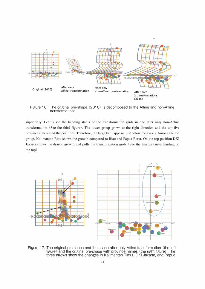
The addition of the two transformations on the original shape makes the 2015 pre-shape. To see the
difference of the scaling, Figure 17 shows the original pre-shape and one after the Affine transformation.
There the same color represents the same province. The Affine transformation shrinks the whole
provinces which means homogenization. Kalimantan Timur and DKI Jakarta relatively decrease in the
Figure 15: Pre-shape change of junior high school percentage and per capita GDP by provinces from 2010 (circle marks) to 2015 (cross marks)
74
superiority. Let us see the bending status of the transformation grids in one after only non-Affine
transformation (See the third figure). The lower group grows to the right direction and the top five
provinces decreased the positions. Therefore, the large bent appears just below the x-axis. Among the top
group, Kalimantan Riau shows the growth compared to Riau and Papua Barat. On the top position DKI
Jakarta shows the drastic growth and pulls the transformation grids (See the hairpin curve bending on
the top).
Figure 16: The original pre-shape (2010) is decomposed to the Affi ne and non-Affi ne transformations.
Figure 17. The original pre-shape and the shape after only Affi ne-transformation (the left fi gure) and the original pre-shape with province names (the right fi gure). The three arrows show the changes in Kalimantan Timur, DKI Jakarta, and Papua.

インドネシア州における教育レベルと GDPの関連の分析(白田)
75
The left figure in Figure 19 illustrates the partial warp #1 change on the original pre-shape. In the right
figure, we extract the net partial warp #1 movement. The change vector of each province makes the
straight line as shown there. In the straight line, the largest negative values are ones of Kalimantan Timur
and DKI Jakarta. On the other hand, the positive growth ones are Maluku, Aceh, D.I Yogyakarta, and
Maluku Utara. The bending status in the partial warp #1 can express most of the non-Affine
transformation.
Then we shall analyze the non-Affine transformation. The non-Affine transformation can be decomposed
to 30 partial warp eigenvectors. Figure 18 shows the eigenvalue amplitude of the original pre-shape
(2010). The value of the first eigenvalue is very large compared to others. Then we can say that the first
partial warp is the dominant one. Let us see the partial warp #1 in Figure 19.
6. ConclusionThis paper has presented an analysis based on the statistical shape analysis of provincial differences in
Indonesia which is based on the economic indicators, i.e. GDP percentage, population percentage, and
electricity by province. The result shows that the education level correlated to a high GDP performance.
In terms of education level by provinces and the GDP percentage, the deformation from 2010 and 2015
shows no significant changes on most of provinces. This result may indicate that the emerging economy
is happening in most of provinces in Indonesia. Moreover, among many level of education. Number of
junior high school graduate in evey provinces has most significant correlation with GDP.
AcknowledgementThis research was partly supported by funds from the Gakushuin University Research Institute for
Economics and Management as the research project in 2018.
Figure 18. Eigenvalue amplitude of the original (2010) pre-shape2015

76
References[1] Oberman, Raoul, et al. “The archipelago economy: Unleashing Indonesia’s potential.” McKinsey Global
Institute. 2012
[2] Hawksworth, John, and Danny Chan. “The World in 2050: Will the shift in global economic power
continue.” PwC’s Economics and Policy (E&P) team in the UK. 2015.
[3] The Economist. Tiger, tiger, almost bright. A guide to Indonesia’s politics and economics in graphics.
https://www.economist.com/graphic-detail/2016/03/04/tiger-tiger-almost-bright
[4] I. L. Dryden and K. V. Mardia, Statistical shape analysis. J. Wiley Chichester, 1998.
[5] K. Mardia, F. Bookstein, and J. Kent, “Alcohol, babies and the death penalty: Saving lives by analysing the
shape of the brain,” Significance, vol. 10, no. 3, pp. 12-16, 2013.
[6] I. L. Dryden and J. T. Kent, Geometry Driven Statistics. Wiley Online Library, 2015.
[7] S. Yukari, H. Takako, and S. Riri Fitri, “Visualization of time series statistical data by shape analysis (GDP
ratio changes among Asia countries),” Journal of Physics: Conference Series, vol. 971, no. 1, p.
Figure 19. Partial warp #1

インドネシア州における教育レベルと GDPの関連の分析(白田)
77
012013, 2018.
[8] Y. Shirota, R. F. Sari, T. Widiyani, and T. Hashimoto, “Visually Do Statistical Shape Analysis! as
TUTORAL,” in Data Science and Advanced Analytics (DSAA) Tokyo, Japan, 2017: IEEE
[9] T. Widiyani, Y. Shirota, and R. F. Sari, “A morphometries analysis method for craniofacial differences of
ancient humans,” in 2017 2nd International Conference on Automation, Cognitive Science, Optics,
Micro Electro-Mechanical System, and Information Technology (ICACOMIT), 2017, pp. 22-27.
[10] Hanushek, Eric A., and Ludger Wößmann. The role of education quality for economic growth. The World
Bank, 2007.
[11] Jasmina, Thia. “Public Spending and Learning Outcomes of Basic Education at the District Level in
Indonesia.” Economics and Finance in Indonesia 62.3. pp.180-190. 2016
[12] World Bank Open Data. Indonesia Percentage of Education Budget to GDP. https://data.worldbank.org/