Embed Size (px)
Citation preview
Central limit theorems and confidence sets in thecalibration of Lévy models and in deconvolution
D I S S E R T A T I O N
zur Erlangung des akademischen Grades
Dr. Rer. Nat.im Fach Mathematik
eingereicht an derMathematisch-Naturwissenschaftlichen Fakultät II
Humboldt-Universität zu Berlin
vonDipl.-Math. Jakob Söhl
Präsident der Humboldt-Universität zu Berlin:Prof. Dr. Jan-Hendrik Olbertz
Dekan der Mathematisch-Naturwissenschaftlichen Fakultät II:Prof. Dr. Elmar Kulke
Gutachter:1. Markus Reiß2. Vladimir Spokoiny3. Richard Nickl
Tag der Verteidigung: 21.03.2013
Abstract
Central limit theorems and confidence sets are studied in two different but relatednonparametric inverse problems, namely in the calibration of an exponential Lévymodel and in the deconvolution model.In the first set–up, an asset is modeled by an exponential of a Lévy process, option
prices are observed and the characteristic triplet of the Lévy process is estimated.We show that the estimators are almost surely well–defined. To this end, we provean upper bound for hitting probabilities of Gaussian random fields and apply thisto a Gaussian process related to the estimation method for Lévy models. We provejoint asymptotic normality for estimators of the volatility, the drift, the intensityand for pointwise estimators of the jump density. Based on these results, we con-struct confidence intervals and sets for the estimators. We show that the confidenceintervals perform well in simulations and apply them to option data of the GermanDAX index.In the deconvolution model, we observe independent, identically distributed ran-
dom variables with additive errors and we estimate linear functionals of the densityof the random variables. We consider deconvolution models with ordinary smootherrors. Then the ill–posedness of the problem is given by the polynomial decay ratewith which the characteristic function of the errors decays. We prove a uniformcentral limit theorem for the estimators of translation classes of linear functionals,which includes the estimation of the distribution function as a special case. Ourresults hold in situations, for which a
√n–rate can be obtained, more precisely, if
the L2–Sobolev smoothness of the functionals is larger than the ill–posedness of theproblem.
ii

Zusammenfassung
Zentrale Grenzwertsätze und Konfidenzmengen werden in zwei verschiedenen,nichtparametrischen, inversen Problemen ähnlicher Struktur untersucht, und zwar inder Kalibrierung eines exponentiellen Lévy–Modells und im Dekonvolutionsmodell.Im ersten Modell wird eine Geldanlage durch einen exponentiellen Lévy–Prozess
dargestellt, Optionspreise werden beobachtet und das charakteristische Tripel desLévy–Prozesses wird geschätzt. Wir zeigen, dass die Schätzer fast sicher wohldefi-niert sind. Zu diesem Zweck beweisen wir eine obere Schranke für Trefferwahrschein-lichkeiten von gaußschen Zufallsfeldern und wenden diese auf einen Gauß–Prozessaus der Schätzmethode für Lévy–Modelle an. Wir beweisen gemeinsame asympto-tische Normalität für die Schätzer von Volatilität, Drift und Intensität und für diepunktweisen Schätzer der Sprungdichte. Basierend auf diesen Ergebnissen konstruie-ren wir Konfidenzintervalle und –mengen für die Schätzer. Wir zeigen, dass sich dieKonfidenzintervalle in Simulationen gut verhalten, und wenden sie auf Optionsdatendes DAX an.Im Dekonvolutionsmodell beobachten wir unabhängige, identisch verteilte Zu-
fallsvariablen mit additiven Fehlern und schätzen lineare Funktionale der Dichteder Zufallsvariablen. Wir betrachten Dekonvolutionsmodelle mit gewöhnlich glattenFehlern. Bei diesen ist die Schlechtgestelltheit des Problems durch die polynomielleAbfallrate der charakteristischen Funktion der Fehler gegeben. Wir beweisen einengleichmäßigen zentralen Grenzwertsatz für Schätzer von Translationsklassen linearerFunktionale, der die Schätzung der Verteilungsfunktion als Spezialfall enthält. Un-sere Ergebnisse gelten in Situationen, in denen eine
√n–Rate erreicht werden kann,
genauer gesagt gelten sie, wenn die L2–Sobolev–Glattheit der Funktionale größer alsdie Schlechtgestelltheit des Problems ist.
iii

Contents
1 Introduction 1
2 Calibration of exponential Lévy models 72.1 Lévy processes . . . . . . . . . . . . . . . . . . . . . . . . . . . . . . . . . 72.2 Spectral calibration method . . . . . . . . . . . . . . . . . . . . . . . . . . 82.3 The misspecified model . . . . . . . . . . . . . . . . . . . . . . . . . . . . 142.4 Preliminary error analysis . . . . . . . . . . . . . . . . . . . . . . . . . . . 16
3 On a related Gaussian process 193.1 Continuity and boundedness . . . . . . . . . . . . . . . . . . . . . . . . . . 203.2 Hitting probabilities . . . . . . . . . . . . . . . . . . . . . . . . . . . . . . 23
3.2.1 General results . . . . . . . . . . . . . . . . . . . . . . . . . . . . . 253.2.2 Application . . . . . . . . . . . . . . . . . . . . . . . . . . . . . . . 273.2.3 Proof of Lemma 3.6 . . . . . . . . . . . . . . . . . . . . . . . . . . 28
4 Asymptotic normality 334.1 Main results . . . . . . . . . . . . . . . . . . . . . . . . . . . . . . . . . . . 334.2 Discussion of the results . . . . . . . . . . . . . . . . . . . . . . . . . . . . 384.3 Proof of the asymptotic normality . . . . . . . . . . . . . . . . . . . . . . 39
4.3.1 The linearized stochastic errors . . . . . . . . . . . . . . . . . . . . 394.3.2 The remainder term . . . . . . . . . . . . . . . . . . . . . . . . . . 474.3.3 The approximation errors . . . . . . . . . . . . . . . . . . . . . . . 49
5 Uniformity with respect to the underlying probability measure 515.1 General approach . . . . . . . . . . . . . . . . . . . . . . . . . . . . . . . . 515.2 Uniformity in the case σ = 0 . . . . . . . . . . . . . . . . . . . . . . . . . 565.3 Uniformity in the case σ > 0 . . . . . . . . . . . . . . . . . . . . . . . . . 595.4 Uniformity for the remainder term . . . . . . . . . . . . . . . . . . . . . . 60
6 Applications 636.1 Construction of confidence intervals and confidence sets . . . . . . . . . . 636.2 Inference on the volatility . . . . . . . . . . . . . . . . . . . . . . . . . . . 66
7 Simulations and empirical results 717.1 The estimation method in applications . . . . . . . . . . . . . . . . . . . . 727.2 Simulations . . . . . . . . . . . . . . . . . . . . . . . . . . . . . . . . . . . 747.3 Confidence intervals . . . . . . . . . . . . . . . . . . . . . . . . . . . . . . 76
v
Contents
7.4 Empirical study . . . . . . . . . . . . . . . . . . . . . . . . . . . . . . . . . 797.5 Finite sample variances of γ, λ and ν . . . . . . . . . . . . . . . . . . . . . 82
8 A uniform central limit theorem for deconvolution estimators 878.1 The estimator . . . . . . . . . . . . . . . . . . . . . . . . . . . . . . . . . . 888.2 Statement of the theorem . . . . . . . . . . . . . . . . . . . . . . . . . . . 898.3 Discussion . . . . . . . . . . . . . . . . . . . . . . . . . . . . . . . . . . . . 928.4 The deconvolution operator . . . . . . . . . . . . . . . . . . . . . . . . . . 958.5 Convergence of the finite dimensional distributions . . . . . . . . . . . . . 97
8.5.1 The bias . . . . . . . . . . . . . . . . . . . . . . . . . . . . . . . . . 978.5.2 The stochastic error . . . . . . . . . . . . . . . . . . . . . . . . . . 98
8.6 Tightness . . . . . . . . . . . . . . . . . . . . . . . . . . . . . . . . . . . . 1008.6.1 Pregaussian limit process . . . . . . . . . . . . . . . . . . . . . . . 1018.6.2 Uniform central limit theorem . . . . . . . . . . . . . . . . . . . . . 1038.6.3 The critical term . . . . . . . . . . . . . . . . . . . . . . . . . . . . 105
8.7 Function spaces . . . . . . . . . . . . . . . . . . . . . . . . . . . . . . . . . 108
9 Conclusion and outlook 111
Acknowledgements 115
Bibliography 117
vi
1 Introduction
Central limit theorems for estimators are of fundamental interest since they allow toassess the reliability of estimators and to construct confidence sets which cover theunknown parameters or functions with a prescribed probability. We focus on nonpara-metric inverse problems and study two different but related models. In the first one, anasset price is modeled by an exponential of a Lévy process. Option prices of the assetare observed and the aim is to estimate the characteristic triplet of the Lévy process.The second model is deconvolution, where independent, identically distributed randomvariables with additive error are observed and the aim is statistical inference on thedistribution of the random variables.In both models, in the estimation of the Lévy process and in the deconvolution, we
study central limit theorems for estimators that are based on Fourier methods. In the firstset–up, the price of an asset (St) follows under the risk–neutral measure an exponentialLévy model
St = Sert+Lt with a Lévy process (Lt) for t > 0,
where S > 0 the present value of the stock and r > 0 is the riskless interest rate.Based on prices of European options with the underlying (St), we calibrate the modelby estimating the characteristic triplet of (Lt), which consists of the volatility, the driftand the Lévy measure. We construct confidence sets for the characteristic triplet. This isof particular importance since the calibrated model is the basis for pricing and hedging.The calibration problem is closely related to the classical nonparametric inverse problemof deconvolution. On the one hand the law of the continuous part is convolved with thelaw of the jump part of the Lévy process. On the other hand the Lévy measure isconvolved with itself in the marginal distribution of the jump part. Besides being itselfan interesting problem with many applications, the deconvolution model exhibits thesame underlying structure as the nonlinear estimation of the characteristic triplet of aLévy process and is easier to analyze since it is linear. In the deconvolution model, weobserve n random variables
Yj = Xj + εj , j = 1, . . . , n,
where the Xj are identically distributed with density fX , the εj are identically dis-tributed with density fε and where X1, . . . , Xn, ε1, . . . , εn are independent. The aim isto estimate the distribution function of the Xj or, more precisely, linear functionals∫ζ(x − t)fX(x) dx of the density fX , where the special case ζ = 1(−∞,0] leads to the
estimation of the distribution function. Since the central limit theorems show that the
1
1 Introduction
estimators are asymptotically normally distributed, we also speak of asymptotic normal-ity. In both problems, we determine the joint asymptotic distribution of the estimators.In the deconvolution problem, we even prove a uniform central limit theorem mean-ing that the asymptotic normality holds uniformly over all t ∈ R. Based on the jointasymptotic distribution of the estimators, we construct confidence intervals and jointconfidence sets. The uniform convergence in the deconvolution paves the way for theconstruction of confidence bands.Lévy processes are widely used in financial modeling, since they allow to reproduce
many stylized facts well. Exponential Lévy models generalize the classical model byBlack and Scholes (1973) by accounting in addition to volatility and drift for jumps inthe price process. They are capable of modeling not only a volatility smile or skew butalso the effect that the smile or skew is more pronounced for shorter maturities. For arecent review on pricing and hedging in exponential Lévy models see Tankov (2011).The calibration of exponential Lévy models has mainly focused on parametric models,cf. Barndorff-Nielsen (1998); Carr et al. (2002); Eberlein et al. (1998) and the referencestherein. First nonparametric calibration procedures for Lévy models were proposed byCont and Tankov (2004b, 2006) as well as by Belomestny and Reiß (2006a). In theseapproaches no parametrization is assumed on the jump density and thus the model mis-specification is reduced. In both methods, the calibration is based on prices of Europeancall and put options. Cont and Tankov introduce a least squares estimator penalizedby relative entropy. Belomestny and Reiß propose the spectral calibration method andshow that it achieves the minimax rates of convergence. The spectral calibration methodis designed for finite intensity Lévy processes with Gaussian component and it is basedon a regularization by a spectral cut–off. We show asymptotic normality as well as con-struct confidence sets and intervals for the spectral calibration method. Similar methodswere also applied by Belomestny (2010) to estimate the fractional order of regular Lévyprocesses of exponential type, by Belomestny and Schoenmakers (2011) to calibrate aLibor model and by Trabs (2012) to estimate self–decomposable Lévy processes.The estimation of Lévy processes from direct observations has been studied for high–
frequency and for low–frequency observations. For high–frequency observations the timebetween observations tends to zero as the number of observations grows, while for low–frequency observations the time between observations is fixed. As a starting point forhigh–frequency observations, Figueroa-López and Houdré (2006) estimate a Lévy pro-cess nonparametrically from continuous observations. Nonparametric estimation fromdiscrete observations at high frequency is treated by Figueroa-López (2009) or by Comteand Genon-Catalot (2009, 2011). Nonparametric estimation of Lévy processes from low–frequency observations has been studied for the estimation of functionals by Neumannand Reiß (2009), for finite intensity Lévy processes with Gaussian component by Gu-gushvili (2009) or for pure jump Lévy processes of finite variation via model selectionby Comte and Genon-Catalot (2010) and by Kappus (2012).We prove asymptotic normality for the spectral calibration method, where the Lévy
process is observed only indirectly since the method is based on option prices. Theindirect observation scheme does not correspond to direct observations at high frequency
2
but at low frequency. Our asymptotic normality results are for estimators of the volatility,the drift, the intensity and pointwise for estimators of the jump density. These theoremson asymptotic normality belong to the main results of this thesis and are also available inSöhl (2012). This calibration problem is a statistical inverse problem, which is completelydifferent in the mildly ill–posed case of volatility zero and in the severely ill–posedcase of positive volatility. We treat both cases. A confidence set is called honest if thelevel is achieved uniformly over a class of the estimated objects. We prove asymptoticnormality uniformly over a class of characteristic triplets and use this to construct honestconfidence intervals. The asymptotic normality results are based on undersmoothing andon a linearization of the stochastic errors. As it turns out the asymptotic distribution iscompletely determined by the linearized stochastic errors.Based on the asymptotic analysis, we construct confidence intervals from the finite
sample variance of the linearized stochastic errors. We study the performance of theconfidence intervals in simulations and apply the confidence intervals to option data ofthe German DAX index. While we focus in this thesis on the spectral calibration methodby Belomestny and Reiß (2006a), the approach can be easily generalized to similarmethods. The construction of the confidence sets, the simulations and the empiricalstudy will appear in Söhl and Trabs (2012b), where this is also carried out for themethod by Trabs (2012).Nonparametric confidence intervals and sets for jump densities have been studied by
Figueroa-López (2011). The method is based on direct high–frequency observations sothat the statistical problem of estimating the jump density is easier than in our set–up.On the other hand the results yield beyond pointwise confidence intervals also confidencebands.For low–frequency observations, Nickl and Reiß (2012) show in a recent paper a central
limit theorem for the nonparametric estimation of Lévy processes. They consider theestimation of the generalized distribution function of the Lévy measure in the mildlyill–posed case for particular situations in which a
√n–rate can be obtained and prove a
uniform central limit theorem for their estimators.So while central limit theorems have been treated in the nonparametric estimation
of Lévy processes for low–frequency observations in the mildly ill–posed case, there areto the best of the author’s knowledge no results in the severely ill–posed case and ourresults are the first for this case.The estimation of the characteristic triplet from low–frequency observations of a Lévy
processes is closely related to the deconvolution problem. Considering the deconvolutionproblem for two different densities fX and fX yields equation (8.2), namely
F [fX − fX ](u) = ϕ(u)− ϕ(u)ϕε(u) , (1.1)
where ϕ and ϕ are the characteristic functions of the observations belonging to fX andfX , respectively, and ϕε is the characteristic function of the errors εj . The correspondingformula (2.28) for two characteristic triplets of a Lévy process exhibits the same struc-ture. The difference is that there ϕ and ϕε are both replaced by the same characteristic
3
1 Introduction
function ϕT of the Lévy process. This is called auto–deconvolution, since the distributionof the errors is replaced by the marginal distribution of the Lévy process itself. Fromthe structure of the above formula one can also see that the decay of the characteristicfunctions ϕε and ϕT , respectively, determines the ill–posedness of the problems. A poly-nomial decay corresponds to the mildly ill–posed case and an exponential decay to theseverely ill–posed case.We consider the deconvolution problem in the mildly ill–posed case, which is the
deconvolution problem with ordinary smooth errors. Using kernel estimators, we estimatelinear functionals
∫ζ(x− t)fX(x) dx, which are general enough to include the estimation
of the distribution function as a special case. Our main result in the deconvolutionproblem is a central limit theorem for the estimators uniformly over all t ∈ R. Thisresult will appear in Söhl and Trabs (2012a), where in addition also the efficiency of theestimators is shown. Similarly to the situation considered by Nickl and Reiß (2012) forLévy processes, we treat the case where a
√n–rate can be obtained. Our work gives a
clear insight into the interplay between the smoothness of ζ and the ill–posedness of theproblem. A
√n–rate can be obtained whenever the smoothness of ζ in an L2–Sobolev
sense compensates the ill–posedness of the problem determined by the polynomial rate bywhich the characteristic function of the error decays. The limit process G in the uniformcentral limit theorem is a generalized Brownian bridge, whose covariance depends on thefunctional ζ and through the deconvolution operator F−1[1/ϕε] also on the distributionof the error. By uniform convergence the kernel estimator of fX fulfills the ‘plug–in’property of Bickel and Ritov (2003). The theory of smoothed empirical processes astreated in Radulović and Wegkamp (2000) as well as in Giné and Nickl (2008) is usedto prove the uniform central limit theorem.Deconvolution is a well studied problem. So we focus here only on the closely related
literature and refer to the references therein for further reading. Fan (1991b) treatsminimax convergence rates for estimating the density and the distribution function. Bu-tucea and Comte (2009) treat the data–driven choice of the bandwidth for estimatinglinear functionals of the density fX , but assume some minimal smoothness and inte-grability conditions on the functional, which exclude, for example, the estimation ofthe distribution function since 1(−∞,t] is not integrable. Dattner et al. (2011) study theminimax–optimal and adaptive estimation of the distribution function.In view of our work, we focus now on asymptotic normality and on confidence sets.
Deconvolution is generally considered in the mildly ill–posed case of ordinary smootherrors and in the severely ill–posed case of supersmooth errors. In ordinary smoothdeconvolution, asymptotic normality is shown for the estimation of the density by Fan(1991a) and on slightly weaker assumptions by Fan and Liu (1997). For the estimation ofthe distribution function, Hall and Lahiri (2008) show asymptotic normality in ordinarysmooth deconvolution. In supersmooth deconvolution, asymptotic normality is provedfor estimators of the density by Zhang (1990) and by Fan (1991a). Zhang (1990) coversalso estimators of the distribution function and van Es and Uh (2005) further determinethe asymptotic behavior of the variance for estimators of the density and of the dis-tribution function in supersmooth deconvolution. The asymptotic normality results on
4
supersmooth deconvolution are extended by van Es and Uh (2004) to the case when thecharacteristic function of the errors decays exponentially but possibly slower than theone of the Cauchy distribution. Further developing the work by Bickel and Rosenblatt(1973) on density estimation, Bissantz et al. (2007) construct confidence bands for thedensity in ordinary smooth deconvolution. Lounici and Nickl (2011) give uniform riskbounds for wavelet density estimators in the deconvolution problem, which can be usedto construct nonasymptotic confidence bands.In both problems, we apply spectral regularization. The higher the frequencies, the
more they contribute to the stochastic error. We regularize by discarding all frequencieshigher than a certain cut–off value. Since we regularize in the spectral domain, Fouriertechniques are used for the estimation methods and their analysis.Another common feature is that Gaussian processes arise naturally in both problems.
The limit process of the stochastic error in the deconvolution problem is a generalizedBrownian bridge. The problem of estimating the characteristic triplet of a Lévy processcan be simplified by studying observations in the Gaussian white noise model. Applyingthe estimation method to this modified observation scheme leads to a Gaussian process.A bound on the supremum of this Gaussian process is derived which is later used toprove asymptotic normality of the estimators. For the Gaussian processes in both prob-lems, we study boundedness and continuity using Dudley’s theorem and metric entropyarguments. While these are classical topics in the theory of Gaussian processes, we alsoaddress the question of hitting probabilities for Gaussian processes or, more generally,for Gaussian random fields. These results on hitting probabilities are of independentinterest and are published in Söhl (2010). They are used to show that points are polarfor the Gaussian process resulting from the Gaussian white noise model meaning thatit does not hit a given point almost surely. This implies that the estimators in the Lévysetting are almost surely well–defined.In both problems, in the deconvolution and in the estimation of the Lévy process,
we use nonparametric estimation methods. The estimation errors can be decomposedinto a stochastic and an approximation part. Unlike the bias–variance trade–off sug-gests, we do not try to balance stochastic and approximation error but rather aim forundersmoothing. Then the approximation error is asymptotically negligible and thus theasymptotic distribution is centered around the true value. The asymptotic variance canbe easily estimated by means of the already used estimators. In contrast to a bias cor-rection, which often leads to more difficult estimation problems, undersmoothing yieldsaccessible asymptotic distributions and feasible confidence sets.This thesis is organized as follows. Chapter 2 treats the exponential Lévy model and
the spectral estimation method. Chapter 3 studies continuity, boundedness and hit-ting probabilities of a related Gaussian process. Chapter 4 contains the main results onasymptotic normality in the Lévy setting. Chapter 5 treats uniform convergence withrespect to the underlying probability measure. In Chapter 6 the asymptotic normalityresults are applied to confidence sets and to a hypotheses test on the value of the volatil-ity. Chapter 7 contains a finite sample analysis, simulations and an empirical study onthe calibration of the exponential Lévy model. Chapter 8 treats the deconvolution model
5

1 Introduction
and is devoted to a uniform central limit theorem for estimators of linear functionals ofthe density. We conclude and give an outlook on further research topics in Chapter 9.
6
2 Calibration of exponential Lévy models
This chapter introduces the spectral calibration method and begins to analyze the esti-mation error. To this end, we provide some background on Lévy processes in Section 2.1.We describe the spectral calibration method and a slight modification thereof both byBelomestny and Reiß (2006a,b) in Section 2.2, where we also briefly discuss the struc-tural similarity of the calibration and the deconvolution problem. In Section 2.3, anexample of model misspecification is considered. We introduce an error decompositionin Section 2.4 which will be important later for the further analysis of the errors.
2.1 Lévy processesIn this section, we define Lévy processes and summarize some of their properties, whichcan be found, for example, in the monograph by Sato (1999). Later we will need onlyone dimensional Lévy processes. Nevertheless, we treat here Lévy processes with valuesin Rd since this causes no additional effort.
Definition 2.1 (Lévy process). An Rd–valued stochastic process (Lt)t>0 on probabilityspace (Ω,F ,P) is called a Lévy process if the following properties are satisfied:
(i) L0 = 0 almost surely,
(ii) (Lt) has independent increments: for any choice of n > 1 and 0 6 t0 < t1 < · · · < tnthe random variables Lt0 , Lt1 − Lt0 , . . . , Ltn − Ltn−1 are independent,
(iii) (Lt) has stationary increments: the distribution of Lt+s−Lt does not depend on t,
(iv) (Lt) is stochastically continuous: for all t > 0, ε > 0, lims→0 P(|Lt+s−Lt| > ε) = 0,
(v) (Lt) has almost surely càdlàg paths: there exists Ω0 ∈ F with P(Ω0) = 1 such thatfor all ω ∈ Ω0, Lt(ω) is right–continuous at all t > 0 and has left limits at all t > 0.
Example 2.2. (i) A Brownian motion with a deterministic drift (ΣBt+γt) is a Lévyprocess, where Σ ∈ Rd×d, γ ∈ Rd and Bt is a d–dimensional Brownian motion.
(ii) A Poisson process (Nt) of intensity λ > 0 is a Lévy process. More generally,the compound Poisson process (Yt) is a Lévy process, where Yt :=
∑Ntj=1 Zj with
independent, identically distributed random variables Zj , which take values in Rd.
We note that the sum of two independent Lévy processes is again a Lévy process.These examples capture the behavior of Lévy processes quite well. Indeed, the Lévy–Itô decomposition states that any Lévy process can be represented as the sum of three
7
2 Calibration of exponential Lévy models
independent components L = L1 + L2 + L3, where L1 is a Brownian motion with de-terministic drift, L2 is a compound Poisson process with jumps larger or equal to oneand L3 is a martingale representing the possible infinitely many jumps smaller than one,which may be obtained as the limit of compensated compound Poisson processes withjumps smaller than one. We call L1 the continuous part and L2 + L3 the jump part ofthe Lévy process. For a precise formulation of the Lévy–Itô decomposition and a proofwe refer to Sato (1999). Another main result on Lévy processes is the Lévy–Khintchinerepresentation, whose statement and proof can be found in the same monograph.
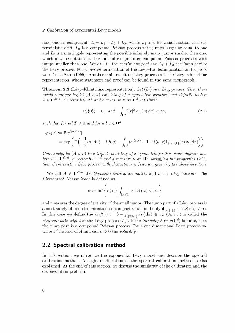
Theorem 2.3 (Lévy–Khintchine representation). Let (Lt) be a Lévy process. Then thereexists a unique triplet (A, b, ν) consisting of a symmetric positive semi–definite matrixA ∈ Rd×d, a vector b ∈ Rd and a measure ν on Rd satisfying
ν(0) = 0 and∫Rd(|x|2 ∧ 1)ν( dx) <∞, (2.1)
such that for all T > 0 and for all u ∈ Rd
ϕT (u) := E[ei〈u,LT 〉]
= exp(T
(−1
2〈u,Au〉+ i〈b, u〉+∫Rd(ei〈u,x〉 − 1− i〈u, x〉1|x|61(x))ν( dx)
))Conversely, let (A, b, ν) be a triplet consisting of a symmetric positive semi–definite ma-trix A ∈ Rd×d, a vector b ∈ Rd and a measure ν on Rd satisfying the properties (2.1),then there exists a Lévy process with characteristic function given by the above equation.
We call A ∈ Rd×d the Gaussian covariance matrix and ν the Lévy measure. TheBlumenthal–Getoor index is defined as
α := infr > 0
∣∣∣∣∣∫|x|61
|x|rν( dx) <∞
and measures the degree of activity of the small jumps. The jump part of a Lévy process isalmost surely of bounded variation on compact sets if and only if
∫|x|61 |x|ν( dx) <∞.
In this case we define the drift γ := b −∫|x|61 xν( dx) ∈ R. (A, γ, ν) is called the
characteristic triplet of the Lévy process (Lt). If the intensity λ := ν(Rd) is finite, thenthe jump part is a compound Poisson process. For a one dimensional Lévy process wewrite σ2 instead of A and call σ > 0 the volatility.
2.2 Spectral calibration methodIn this section, we introduce the exponential Lévy model and describe the spectralcalibration method. A slight modification of the spectral calibration method is alsoexplained. At the end of this section, we discuss the similarity of the calibration and thedeconvolution problem.
8
2.2 Spectral calibration method
Exponential Lévy models describe the price of an asset by
St = Sert+Lt with a R–valued Lévy process (Lt) for t > 0. (2.2)
A thorough discussion of this model is given in the monograph by Cont and Tankov(2004a). Since the method is based on option prices, the calibration is in the risk neu-tral world modeled by a filtered probability space (Ω,F ,P, (Ft)). We assume that thediscounted price process is a martingale with respect to the risk–neutral measure P andthat under P the price of the asset (St) follows the exponential Lévy model (2.2), whereS > 0 is the present value of the asset and r > 0 is the riskless interest rate.
A European call option with strike price K and maturity T is the right but not theobligation to buy an asset for price K at time T . A European put option is the respectiveright for selling the asset. We denote by C(K,T ) and P(K,T ) the prices of Europeancall and put options which are determined by the pricing formulas
C(K,T ) = e−rT E[(ST −K)+], (2.3)P(K,T ) = e−rT E[(K − ST )+], (2.4)
where we used the notion (A)+ := max(A, 0). Subtracting (2.4) from (2.3) yields thewell known put–call parity
C(K,T )− P(K,T ) = S − e−rTK,
where we used that (e−rtSt) is a martingale. By the put–call parity, call prices can becalculated into put prices and vice versa so that the observation may be given by eitherof them. We fix some T and suppose that the observed option prices correspond todifferent maturities (Kj) and are given by the value of the pricing formula corrupted bynoise:
Yj = C(Kj , T ) + ηjξj , j = 1, . . . , n. (2.5)
The minimax result in Belomestny and Reiß (2006a) is shown for general errors (ξj)which are independent, centered random variables with Var(ξj) = 1 and supj E[ξ4
j ] <∞.The observation errors are due to the bid–ask spread and other market frictions. Thenoise levels (ηj) can be either determined from the bid–ask spread, which indicates byCont and Tankov (2004a, p. 438/439) how reliable an observation is, or they can beestimated nonparametrically, for example, with the method by Fan and Yao (1998). Wetransform the observations to a regression problem on the function
O(x) :=S−1C(x, T ), x > 0,S−1P(x, T ), x < 0,
where x := log(K/S)− rT denotes the negative log–forward moneyness. The regressionmodel may then be written as
Oj = O(xj) + δjξj , (2.6)
9
2 Calibration of exponential Lévy models
where δj = S−1ηj . Since the design may change with n, it would be more precise to indexthe regression model (2.6) by nj instead of by j only. But for notational convenience weomit the dependence on n.
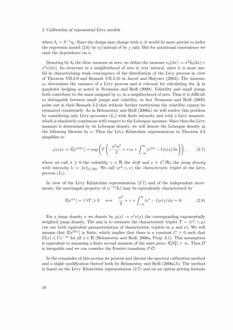
Denoting by δ0 the dirac measure at zero, we define the measure νσ(dx) := σ2δ0(dx)+x2ν(dx). Its structure in a neighborhood of zero is very natural, since it is most use-ful in characterizing weak convergence of the distribution of the Lévy process in viewof Theorem VII.2.9 and Remark VII.2.10 in Jacod and Shiryaev (2003). The measureνσ determines the variance of a Lévy process and is relevant for calculating the ∆ inquadratic hedging as noted in Neumann and Reiß (2009). Volatility and small jumpsboth contribute to the mass assigned by νσ to a neighborhood of zero. Thus it is difficultto distinguish between small jumps and volatility, in fact Neumann and Reiß (2009)point out in their Remark 3.2 that without further restrictions the volatility cannot beestimated consistently. As in Belomestny and Reiß (2006a) we will resolve this problemby considering only Lévy processes (Lt) with finite intensity and with a Lévy measure,which is absolutely continuous with respect to the Lebesgue measure. Since then the Lévymeasure is determined by its Lebesgue density, we will denote the Lebesgue density inthe following likewise by ν. Then the Lévy–Khintchine representation in Theorem 2.3simplifies to
ϕT (u) := E[eiuLT ] = exp(T
(−σ
2u2
2 + iγu+∫ ∞−∞
(eiux − 1)ν(x) dx))
, (2.7)
where we call σ > 0 the volatility, γ ∈ R the drift and ν ∈ L1(R) the jump densitywith intensity λ := ‖ν‖L1(R). We call (σ2, γ, ν) the characteristic triplet of the Lévyprocess (Lt).
In view of the Lévy–Khintchine representation (2.7) and of the independent incre-ments, the martingale property of (e−rtSt) may be equivalently characterized by
E[eLT ] = 1 ∀T > 0 ⇐⇒ σ2
2 + γ +∫ ∞−∞
(ex − 1)ν(x) dx = 0. (2.8)
For a jump density ν we denote by µ(x) := exν(x) the corresponding exponentiallyweighted jump density. The aim is to estimate the characteristic triplet T = (σ2, γ, µ)(we use both equivalent parametrization of characteristic triplets in µ and ν). We willassume that E[e2LT ] is finite, which implies that there is a constant C > 0 such thatO(x) 6 Ce−|x| for all x ∈ R (Belomestny and Reiß, 2006a, Prop. 2.1). This assumptionis equivalent to assuming a finite second moment of the asset price, E[S2
T ] <∞. Then Ois integrable and we can consider the Fourier transform F O.
In the remainder of this section we present and discuss the spectral calibration methodand a slight modification thereof both by Belomestny and Reiß (2006a,b). The methodis based on the Lévy–Khintchine representation (2.7) and on an option pricing formula
10
2.2 Spectral calibration method
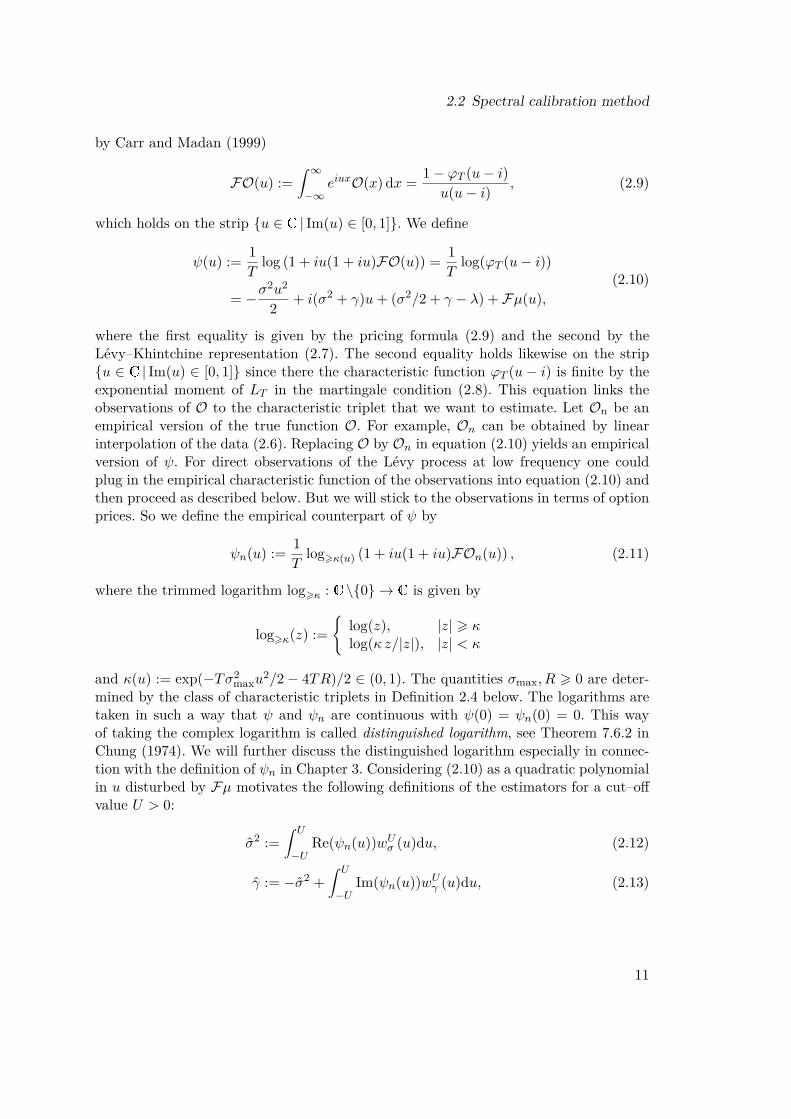
by Carr and Madan (1999)
FO(u) :=∫ ∞−∞
eiuxO(x) dx = 1− ϕT (u− i)u(u− i) , (2.9)
which holds on the strip u ∈ C | Im(u) ∈ [0, 1]. We define
ψ(u) := 1T
log (1 + iu(1 + iu)FO(u)) = 1T
log(ϕT (u− i))
= −σ2u2
2 + i(σ2 + γ)u+ (σ2/2 + γ − λ) + Fµ(u),(2.10)
where the first equality is given by the pricing formula (2.9) and the second by theLévy–Khintchine representation (2.7). The second equality holds likewise on the stripu ∈ C | Im(u) ∈ [0, 1] since there the characteristic function ϕT (u − i) is finite by theexponential moment of LT in the martingale condition (2.8). This equation links theobservations of O to the characteristic triplet that we want to estimate. Let On be anempirical version of the true function O. For example, On can be obtained by linearinterpolation of the data (2.6). Replacing O by On in equation (2.10) yields an empiricalversion of ψ. For direct observations of the Lévy process at low frequency one couldplug in the empirical characteristic function of the observations into equation (2.10) andthen proceed as described below. But we will stick to the observations in terms of optionprices. So we define the empirical counterpart of ψ by
ψn(u) := 1T
log>κ(u) (1 + iu(1 + iu)FOn(u)) , (2.11)
where the trimmed logarithm log>κ : C \0 → C is given by
log>κ(z) :=
log(z), |z| > κlog(κ z/|z|), |z| < κ
and κ(u) := exp(−Tσ2maxu
2/2− 4TR)/2 ∈ (0, 1). The quantities σmax, R > 0 are deter-mined by the class of characteristic triplets in Definition 2.4 below. The logarithms aretaken in such a way that ψ and ψn are continuous with ψ(0) = ψn(0) = 0. This wayof taking the complex logarithm is called distinguished logarithm, see Theorem 7.6.2 inChung (1974). We will further discuss the distinguished logarithm especially in connec-tion with the definition of ψn in Chapter 3. Considering (2.10) as a quadratic polynomialin u disturbed by Fµ motivates the following definitions of the estimators for a cut–offvalue U > 0:
σ2 :=∫ U
−URe(ψn(u))wUσ (u)du, (2.12)
γ := −σ2 +∫ U
−UIm(ψn(u))wUγ (u)du, (2.13)
11
2 Calibration of exponential Lévy models
λ := σ2
2 + γ −∫ U
−URe(ψn(u))wUλ (u)du, (2.14)
where the weight functions wUσ , wUγ and wUλ satisfy
∫ U
−U
−u2
2 wUσ (u)du = 1,∫ U
−UuwUγ (u)du = 1,
∫ U
−UwUλ (u)du = 1,∫ U
−UwUσ (u)du = 0,
∫ U
−Uu2wUλ (u)du = 0.
(2.15)
The estimator for µ is defined by a smoothed inverse Fourier transform of the remainder
µ(x) := F−1[(ψn(u) + σ2
2 (u− i)2 − iγ(u− i) + λ
)wUµ (u)
](x), (2.16)
where wUµ is compactly supported. The choice of the weight functions is discussed inSection 7.1, where also possible weight functions are given. The weight functions for allU > 0 can be obtained from w1
σ, w1γ , w1
λ and w1µ by rescaling:
wUσ (u) = U−3w1σ(u/U), wUγ (u) = U−2w1
γ(u/U),wUλ (u) = U−1w1
λ(u/U), wUµ (u) = w1µ(u/U).
Since ψn(−u) = ψn(u), only the symmetric part of w1σ, w1
λ and the antisymmetric part ofw1γ matter. The antisymmetric part of w1
µ contributes a purely imaginary part to µ(x).Without loss of generality we will always assume w1
σ, w1λ, w1
µ to be symmetric and w1γ
to be antisymmetric. We further assume that the supports of w1σ, w1
γ , w1λ and w1
µ arecontained in [−1, 1].To bound the approximation errors some smoothness assumption is necessary. We
assume that the characteristic triplet belongs to a smoothness class given by the followingdefinition, which is Definition 4.1 by Belomestny and Reiß (2006a).
Definition 2.4. For s ∈ N and R, σmax > 0 let Gs(R, σmax) denote the set of allcharacteristic triplets T = (σ2, γ, µ) such that (eLt) is a martingale, E[e2LT ] 6 R holds,µ is s–times (weakly) differentiable and
σ ∈ [0, σmax], |γ|, λ ∈ [0, R], max06k6s
‖µ(k)‖L2(R) 6 R, ‖µ(s)‖L∞(R) 6 R.
The assumption T ∈ Gs(R, σmax) includes a smoothness assumption of order s on µleading to a decay of Fµ. To profit from this decay when bounding the approximationerror in Section 4.3.3, we assume that the weight functions are of order s, this means
F(w1σ(u)/us),F(w1
γ(u)/us),F(w1γ(u)/us),F((1− w1
µ(u))/us) ∈ L1(R). (2.17)
A slightly modified estimation method is given in a second paper by Belomestny andReiß (2006b), which is concerned with simulations and an empirical example. We present
12

2.2 Spectral calibration method
this approach here for completeness and since our simulations and our empirical studyare partly based on it. In addition, we will apply the modified method to an exampleand this will shed some light on misspecification in the next section. As noted, theequation (2.10) holds on the whole strip u ∈ C | Im(u) ∈ [0, 1]. So instead of usingthis equation directly one could also shift the equation. A shift by one in the imaginarydirection is particularly appealing, since then ν can be estimated directly without theintermediate step of estimating an exponentially scaled version of ν. Applying this shiftto (2.10) yields
ψ(u+ i) = 1T
log(1− u(u+ i)F O(u+ i)) = 1T
log(ϕT (u))
= −σ2u2
2 + iγu− λ+ F ν(u).(2.18)
Similar as for equation (2.10), one could also plug in an empirical characteristic functionobtained from direct, low–frequency observations here. This is exactly the approachGugushvili (2009) takes. But we notice F O(u+i) = F [e−xO(x)](u). Again we substituteO by its empirical counterpart On and define
ψn(u+ i) := 1T
log(1− u(u+ i)F [e−xOn(x)](u)). (2.19)
So the slightly modified estimators are given by
σ2 :=∫ U
−URe(ψn(u+ i))wUσ (u)du, (2.20)
γ :=∫ U
−UIm(ψn(u+ i))wUγ (u)du, (2.21)
λ := −∫ U
−URe(ψn(u+ i))wUλ (u)du, (2.22)
where the weight functions are assumed to satisfy the same conditions (2.15) as before.The corresponding estimator of ν is
ν(x) := F−1[(ψn(u+ i) + σ2
2 u2 − iγu+ λ
)wUν (u)
](x), (2.23)
where wUν is compactly supported. Belomestny and Reiß (2006b) proposed the weightfunctions
wUσ (u) := s+ 31− 2−2/(s+1)U
−(s+3)|u|s(1− 2 · 1|u|>2−1/(s+1)U), u ∈ [−U,U ], (2.24)
wUγ (u) := s+ 22U s+2 |u|
s sgn(u), u ∈ [−U,U ], (2.25)
wUλ (u) := s+ 12(22/(s+3) − 1)
U−(s+1)|u|s(2 · 1|u|<2−1/(s+3)U − 1), u ∈ [−U,U ], (2.26)
13
2 Calibration of exponential Lévy models
wUν (u) := (1− (u/U)2)+, u ∈ R . (2.27)
In order to see the similarity of the estimation of the characteristic triplet of a Lévyprocess with the deconvolution problem we rewrite (2.18) as
T F((σ2/2)δ′′0 − γδ′0 − λδ0 + ν)(u) = log(ϕT (u)).
In the spectral calibration method ϕT is replaced by an empirical version and then thisequation is used to estimate the characteristic triplet. We consider the equation for twodifferent characteristic triplets (σ, γ, ν) and (σ, γ, ν) with intensities λ and λ, respectively,and obtain
T F(((σ2 − σ2)/2)δ′′0 − (γ − γ)δ′0 − (λ− λ)δ0 + (ν − ν))(u)= log(ϕT (u))− log(ϕT (u))
= log(
1 + ϕT (u)− ϕT (u)ϕT (u)
)≈ ϕT (u)− ϕT (u)
ϕT (u) , (2.28)
where the approximation is valid if the absolute value of the last expression is small.This formula reveals the deconvolution structure of the problem. On the one hand thesimilarity with the corresponding formula for deconvolution (1.1) is striking. On theother hand we can see the deconvolution structure directly from formula (2.28). To thisend, we multiply with ϕT on both sides. Since a multiplication in the spectral domaincorresponds to a convolution in the spatial domain, we see that the difference in thecharacteristic triplet is convolved with the marginal distribution of the Lévy process. Toestimate the characteristic triplet a deconvolution problem has to be solved. Interestingly,the marginal distribution of the Lévy process appears twice, it takes the place of both, theerror distribution and the distribution of the observations in the deconvolution problem.This phenomenon is called auto–deconvolution.The linearization of the logarithm in (2.28) will be important later, when we substitute
the logarithm (2.31) in the stochastic errors by its linearization (2.32). Then ϕT will bean empirical version of the characteristic function ϕT , which justifies the assumptionthat ϕT and ϕT are close. The division by the possibly decaying function ϕT is takencare of in the estimation method by the spectral cut–off.
2.3 The misspecified modelWe have chosen a nonparametric estimation method to reduce the error due to modelmisspecification and assume in general that the misspecification error is negligible. Nev-ertheless, model misspecification is an important issue to address. In this section, wewant to study at least by means of an example how the misspecified model behaves.The spectral calibration method is designed for finite intensity Lévy processes. Suddenchanges in the price process are incorporated into the model by jumps of the Lévy pro-cess. The Gaussian component models the small fluctuations happening all the time.Alternatively, one can interpret these fluctuations to be caused by infinitely many small
14
2.3 The misspecified model
jumps. This can be modeled by an infinite intensity Lévy process and empirical inves-tigations indicate that Lévy processes with Blumenthal–Getoor index larger than oneare particularly suitable. Stable processes allow to consider different Blumenthal–Getoorindices α ∈ (0, 2). So we consider a symmetric stable process with additional drift andGaussian component and study the behavior of the estimators for such a process. Thecharacteristic function is given by
ϕT (u) = exp(T (−σ2u2/2− ηα|u|α + iγu)),
where α ∈ (0, 2), σ, η > 0 and γ ∈ R. It holds ψ(u+i) = −σ2u2/2−ηα|u|α+iγu. We takethe weight functions wUσ , wUγ and wUλ as in (2.24), (2.25) and (2.26), respectively, andwUν = 1[−U,U ]. We apply the second method given by (2.20)–(2.23) directly to ψ(u + i)and not to its empirical counterpart ψn(u+ i) and obtain
σ2 =∫ U
−URe(ψ(u+ i))wUσ (u)du = σ2 + 2− 2(s+1−α)/(s+1)
1− 2−2/(s+1)s+ 3
s+ α+ 1ηαU−(2−α),
γ =∫ U
−UIm(ψ(u+ i))wUγ (u)du = γ,
λ = −∫ U
−URe(ψ(u+ i))wUλ (u)du = 2(2−α)/(s+3) − 1
22/(s+3) − 1s+ 1
s+ α+ 1ηαUα,
ν(0) = F−1[(ψ(u+ i) + σ2u2/2− iγu+ λ)1[−U,U ](u)](0)= (−ηαUα+1/(α+ 1) + (σ2 − σ2)U3/6 + λU)/π.
We observe that the drift γ is estimated correctly. The estimated volatility σ2 convergeswith rate U−(2−α) to σ2. The estimated jump intensity is finite, but grows as Uα. Theestimated jump intensity at zero ν(0) grows as Uα+1. Although the estimated jumpintensities are always finite, the infinite intensity of the Lévy process is reflected in theestimators by growing jump intensities and by peaks of growing height at zero. For aLévy process of infinite jump intensity, σ2 has to be interpreted as a joint quantity ofvolatility and small jumps. The corresponding singularity of the jump density is givenby cηα/|x|α+1 with c > 0. The smoothing by the weight function in the spectral domaincorresponds to a kernel smoothing with bandwidth U−1 in the spatial domain. Theintegral of x2ν(x) in a neighborhood of zero with size U−1 is proportional to∫ U−1
−U−1x2ν(x)dx =
∫ U−1
−U−1cηα|x|1−αdx = 2
2− αcηαUα−2.
We see that σ2 behaves as the mass assigned by νσ to a neighborhood of zero withsize proportional to U−1. This example shows that with the above interpretation theestimators can give valuable information about the process even in the case of modelmisspecification.
15
2 Calibration of exponential Lévy models
2.4 Preliminary error analysis
In this section, we start with a preliminary analysis of the error in the correctly specifiedmodel. We decompose the error into an approximation error and a stochastic error. Thestochastic error is further decomposed into a linearized part and a remainder term. Thelinearized stochastic error is considered in the Gaussian white noise model. This leads tothe definition of the Gaussian process studied in Chapter 3. At the same time this errordecomposition lays the ground for the proof of the asymptotic normality in Chapter 4.We define the estimation error ∆σ2 := σ2−σ2 and likewise for the other estimators. We
will also use the notation ∆ψn := ψn−ψ. The estimation error ∆σ2 can be decomposedas
∆σ2 : = 2U2
∫ 1
0Re(Fµ(Uu))w1
σ(u)du+ 2U2
∫ 1
0Re(∆ψn(Uu))w1
σ(u)du. (2.29)
The first term is the approximation error and decreases in the cut–off value U due to thedecay of Fµ. The second is the stochastic error and increases in U by the growth of ∆ψn.For growing sample size n the term ∆ψn becomes smaller so that the stochastic errordecays even if we let U →∞ as n→∞. For σ = 0 the term ∆ψn(u) grows polynomiallyin u so that we can let U tend polynomially to infinity, whereas for σ > 0 it growsexponentially in u and we can let U tend only logarithmically to infinity. This is thereason for the polynomial and logarithmic convergence rates in the cases σ = 0 and σ > 0,respectively. For fixed sample size the cut–off value U is the crucial tuning parameter inthis method and allows a trade–off between the error terms. The influence of the cut–off value U is analogous to the influence of the bandwidth h on kernel estimators, moreprecisely U−1 corresponds to h. The other estimation errors allow similar decompositionsas ∆σ2 in (2.29) and they are given by equations (4.1), (4.2) and (4.3) in the proof ofTheorem 4.1.To simplify the asymptotic analysis of the stochastic errors, we do not work with the
regression model (2.6) but with the Gaussian white noise model. This is an idealizedobservation scheme, where the terms are easier to analyze. At the same time asymptoticresults may be transferred to the regression model. The Gaussian white noise model isgiven by
dZn(x) = O(x)dx+ εnδ(x)dW (x), x ∈ R, (2.30)
where W is a two–sided Brownian motion, δ ∈ L2(R) and εn > 0. In the case ofequidistant design the precise connection to the regression model (2.6) is given byδ(xj) = δj and εn = n+1
n−1(xn − x1)n−1/2, where x1 and xn are the minimal and maxi-mal design points and where we assume that the range of observations (xn − x1) growsslower than n1/2 such that εn → 0 as n → ∞. Transferring asymptotic results fromthe Gaussian white noise model to the regression model is formally justified by LeCam’s concept of asymptotic equivalence, see Le Cam and Yang (2000). In particu-lar, it can be used to transfer lower bounds and confidence statements. Brown and Low(1996) show that the regression (2.6) with Gaussian errors is asymptotically equiva-
16
2.4 Preliminary error analysis
lent to the Gaussian white noise model (2.30). For non–Gaussian errors we refer toGrama and Nussbaum (2002). Their main assumption on the errors is slightly morethan Hellinger differentiability, which is a smoothness assumption on the distributionsof the errors. To be more precise on this asymptotic equivalence, we restrict the Gaus-sian white noise model to a sequence of growing intervals [x1 − ∆n, xn + ∆n] with∆n := (xn − x1)/(n − 1) and assume as a simplification that the observations in theregression model are equidistant with mesh size ∆n. We suppose δ2 > 0 to be an abso-lutely continuous function and | ∂∂x log δ(x)| 6 C to hold for some C <∞. The functionsO are uniformly bounded by O(x) = S−1C(x, T )−(1−ex)+ 6 1 and uniformly Lipschitzby |O′(x)| = |
∫ x−∞O′′(x)dx − 1x>0 + e(γ−λ)T1x>γT,σ=0| 6 4 + eRT , where we used
Proposition 2.1 in Belomestny and Reiß (2006a) and |γ| 6 R. These properties of Oare used to apply Corollary 4.2 in Brown and Low (1996), which yields the asymptoticequivalence of the regression model (2.6) with Gaussian errors and the Gaussian whitenoise model (2.30) each restricted to the intervals [x1 −∆n, xn + ∆n]. In Chapter 7 wewill also treat nonequidistant design in the simulations and in the empirical study. Forthis reason we briefly mention the asymptotic equivalence for nonequidistant design. Tothis end, we consider both models on intervals In := [αn, βn] with limn→∞ αn = −∞and limn→∞ βn = ∞. We assume that there are cumulative distribution functions Hn
on In which are absolutely continuous on In and satisfy H ′n(x) = hn(x) > 0 almosteverywhere on In. The design points are given by xj = H−1(j/(n + 1)), j = 1, . . . , n.Then the regression model (2.6) is asymptotically equivalent to the Gaussian white noisemodel (2.30) where εnδ(x) is replaced by n−1/2δ(x)hn(x)−1/2.The stochastic errors involve the term ∆ψn(Uu), which is a difference between two
logarithms. We define the empirical version of FO by F On := F( dZn). It is obtainedby applying the Fourier transform directly to the Gaussian white noise model (2.30) andthus the intermediate step of constructing an empirical version of O may be omitted.For z, z′ ∈ C \0 and κ > 0 it holds log>κ(z)− log(z′) = log>κ/|z′| (z/z′). That yields
∆ψn(Uu) = 1T
log>κU (u)
(1 + εn iUu(1 + iUu)
1 + iUu(1 + iUu)FO(Uu)
∫ ∞−∞
eiUuxδ(x)dW (x)),
(2.31)
where κU (u) := κ(Uu)/|1 + iUu(1 + iUu)FO(Uu)| 6 1/2, see (Belomestny and Reiß,2006a, (6.3)). We define a linearization Ln,U of the logarithm and the remainder termRn,U by
Ln,U (u) := εn iUu(1 + iUu)T (1 + iUu(1 + iUu)FO(Uu))
∫ ∞−∞
eiUuxδ(x)dW (x), (2.32)
Rn,U (u) := ∆ψn(Uu)− Ln,U (u). (2.33)
This linearization will be an important step in proving asymptotic normality in Chap-ter 4. We will see that on appropriate conditions the linearization Ln,U determinesthe asymptotic distribution of the errors and that the error caused by the remainderterm Rn,U is asymptotically negligible. Ln,U is a Gaussian process and we will devote
17

2 Calibration of exponential Lévy models
the next chapter to the analysis of this Gaussian process.
18
3 On a related Gaussian process
Applying the estimation method to observations in the Gaussian white noise model, leadsnaturally to the Gaussian process Ln,U , which we will study in this chapter. Continuityand boundedness are classical topics in the theory of Gaussian processes and we willinvestigate these properties for Ln,U . In addition, we will treat hitting probabilitiesof Ln,U , which are motivated by the use of the distinguished logarithm in the definitionsof ψ and ψn in (2.10) and (2.11), respectively, as well as by equality (2.31) for ∆ψn.The distinguished logarithm of a function ϕ : [−U,U ] → C with ϕ(0) = 1 exists if it iscontinuous and does not vanish (Chung, 1974, Thm. 7.6.2). The estimators are based onψn and thus implicitly rely on the existence of the distinguished logarithm. Nevertheless,for the estimators σ2, λ and µ(0) the distinguished logarithm may be avoided by usingthe identity Re(log(z)) = log(|z|), so that it suffices to use the usual logarithm of thepositive real numbers. But for the estimators γ and µ(x), x 6= 0, the imaginary partof ψn will in general contribute to the estimators so that the use of the distinguishedlogarithm is essential. The distinguished logarithm in the definition of ψ in (2.10) iswell–defined since ϕT (u − i) is continuous and does not vanish for all u ∈ R, whichcan be seen from the Lévy–Khintchine representation. By ψn = ψ + ∆ψn we concludethat ψn being well–defined is equivalent to ∆ψn being well–defined. The distinguishedlogarithm in the definition of ∆ψn(Uu) in (2.31) is well–defined for u ∈ [−1, 1] wheneverthe argument of the logarithm 1 + TLn,U is continuous and 1 + TLn,U (u) 6= 0 for allu ∈ [−1, 1]. Thus we are interested in conditions ensuring that Ln,U is continuous andthat
Ln,U (u) 6= − 1T
for all u ∈ [−1, 1] (3.1)
either with high probability or almost surely.There is another property of Ln,U that we would like to study. The proofs of the
asymptotic normality results for the estimators rely on the approximation of ∆ψn(Uu) byLn,U (u). This is a good approximation if the argument of the logarithm in the definitionof ∆ψn is close to one, which is equivalent to Ln,U being small. So by bounding Ln,U ,we can bound the remainder Rn,U . Since we are integrating over the unit interval in thedecompositions of the estimation errors (2.29)–(4.3), we will bound Ln,U uniformly onthe unit interval.This chapter is divided into two parts. In Section 3.1 we study continuity and bound-
edness of Ln,U and in Section 3.2 we proof a general result on hitting probabilities andapply it to our situation. This chapter includes the results by Söhl (2010), where mostof the material can be found.
19
3 On a related Gaussian process
3.1 Continuity and boundedness
We first show an auxiliary lemma, where we assume
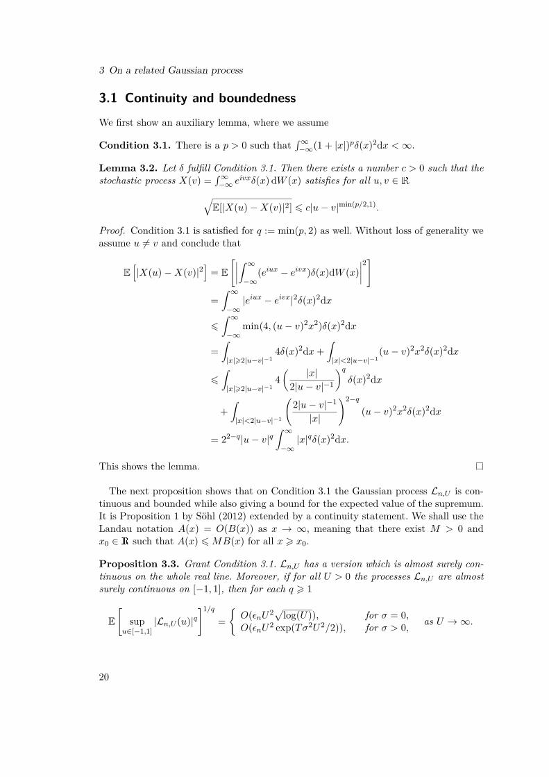
Condition 3.1. There is a p > 0 such that∫∞−∞(1 + |x|)pδ(x)2dx <∞.
Lemma 3.2. Let δ fulfill Condition 3.1. Then there exists a number c > 0 such that thestochastic process X(v) =
∫∞−∞ e
ivxδ(x) dW (x) satisfies for all u, v ∈ R√E[|X(u)−X(v)|2] 6 c|u− v|min(p/2,1).
Proof. Condition 3.1 is satisfied for q := min(p, 2) as well. Without loss of generality weassume u 6= v and conclude that
E[|X(u)−X(v)|2
]= E
[∣∣∣∣∫ ∞−∞
(eiux − eivx)δ(x)dW (x)∣∣∣∣2]
=∫ ∞−∞|eiux − eivx|2δ(x)2dx
6∫ ∞−∞
min(4, (u− v)2x2)δ(x)2dx
=∫|x|>2|u−v|−1
4δ(x)2dx+∫|x|<2|u−v|−1
(u− v)2x2δ(x)2dx
6∫|x|>2|u−v|−1
4( |x|
2|u− v|−1
)qδ(x)2dx
+∫|x|<2|u−v|−1
(2|u− v|−1
|x|
)2−q
(u− v)2x2δ(x)2dx
= 22−q|u− v|q∫ ∞−∞|x|qδ(x)2dx.
This shows the lemma.
The next proposition shows that on Condition 3.1 the Gaussian process Ln,U is con-tinuous and bounded while also giving a bound for the expected value of the supremum.It is Proposition 1 by Söhl (2012) extended by a continuity statement. We shall use theLandau notation A(x) = O(B(x)) as x → ∞, meaning that there exist M > 0 andx0 ∈ R such that A(x) 6MB(x) for all x > x0.
Proposition 3.3. Grant Condition 3.1. Ln,U has a version which is almost surely con-tinuous on the whole real line. Moreover, if for all U > 0 the processes Ln,U are almostsurely continuous on [−1, 1], then for each q > 1
E[
supu∈[−1,1]
|Ln,U (u)|q]1/q
=O(εnU2√log(U)), for σ = 0,O(εnU2 exp(Tσ2U2/2)), for σ > 0, as U →∞.
20
3.1 Continuity and boundedness
Proof. First we define X(u) :=∫∞−∞ e
iuxδ(x)dW (x). Since X(−u) = X(u) it suffices toconsider suprema of the absolute value |X(u)| over positive index sets. We assumed thatthere is an p > 0 such that
∫∞−∞(1 + |x|)pδ(x)2dx < ∞. Lemma 3.2 shows that there
exists a number c > 0 such that√E[|X(u)−X(v)|2] 6 c|u − v|H for all u, v ∈ R with
H := min(p/2, 1) ∈ (0, 1]. Denote by Nρ(I, r) the covering number, that is the minimumnumber of closed balls of radius r in the metric ρ with centers in I that cover I. Wedefine
ρ(u, v) := c|u− v|H
and
d(u, v) :=√E[|X(u)−X(v)|2].
By the above inequality d(u, v) 6 ρ(u, v) for all u, v ∈ R. A ball of radius r in the metricρ covers an interval of length 2(r/c)1/H . Thus, it holds
Nρ([0, U ], r) =⌈U (c/r)1/H /2
⌉,
where dae is the smallest integer equal or larger than a. The radius of the smallest ballwith center in [0, U ] that contains [0, U ] is c(U/2)H with respect to the metric ρ. Thereexists D < ∞ such that d(u, v) 6 D for all u, v ∈ R. For U large enough such thatU > (D/c)1/H we have the entropy bound
J([0, U ], d) :=∫ ∞
0(log(Nd([0, U ], r)))1/2 dr =
∫ D
0(log(Nd([0, U ], r)))1/2 dr
6∫ D
0(log(Nρ([0, U ], r)))1/2 dr 6
∫ D
0
(log
(U (c/r)1/H
))1/2dr (3.2)
6 H−1/2∫ D
0
(log
(UHc/r
))1/2dr,
here we substitute r = UHcs,
6 H−1/2UHc
∫ D/(UHc)
0(log (1/s))1/2 ds. (3.3)
This integral is solved by∫ x
0
√log y−1dy =
√π
2 −√π
2 Erf(√
log x−1) + x√
log x−1,
where Erf(y) = 2√π
∫ y0 e−t2dt. For all y > 0 the estimate 1 − Erf(y) 6 exp(−y2)/(
√πy)
holds, which is a standard estimate for the c.d.f. of the Gaussian distribution, seeLemma 22.2 in Klenke (2007).
21
3 On a related Gaussian process
For each H > 0 this yields c > 0 such that for all x ∈ (0, 1/2H)∫ x
0
√log y−1dy 6 cx
√log x−1.
Thus, (3.3) can be bounded by
(H−1/2cD)√
log(UHc/D) = O((logU)1/2)
as U → ∞. Consequently, (logU)1/2 is an asymptotic upper bound of the entropyintegral (3.2). By Dudley’s theorem (e.g., see Kahane, 1985, p. 219) there is for allU > 0 a version of X which is almost surely continuous on [−U,U ] with respect to dand by Lemma 3.2 also with respect to the Euclidean metric. Two versions of the samestochastic process are indistinguishable if they are both almost surely continuous and ifthe index set is an interval (Klenke, 2007, Lem. 21.5). Thus, there is a version of X andsubsequently of Ln,U which is almost surely continuous with respect to the Euclideanmetric on R.Let X ′ be an almost surely continuous version of X. Then
εniUu(1 + iUu)1 + iUu(1 + iUu)F O(Uu)X
′(Uu) (3.4)
is an almost surely continuous version of Ln,U . If Ln,U is almost surely continuous on[−1, 1] then Ln,U and the process (3.4) are indistinguishable on [−1, 1].Dudley’s theorem yields for all q > 1
E[
supu∈[−U,U ]
|Re(X ′(u))|q]
= O((logU)q/2) (3.5)
and
E[
supu∈[−U,U ]
| Im(X ′(u))|q]
= O((logU)q/2)
as U →∞. We estimate from above for all q > 1
E[
supu∈[−1,1]
|Ln,U (u)|q]
6 supu∈[−U,U ]
∣∣∣∣ εniu(1 + iu)T (1 + iu(1 + iu)FO(u))
∣∣∣∣q E[
supu∈[0,U ]
|X ′(u)|q]
6
(εnU√
1 + U2
T exp(T (−σ2U2/2 + σ2/2 + γ − λ− ‖Fµ‖∞))
)qE[
supu∈[0,U ]
|X ′(u)|q]
= O
((εnU
2√
log(U) exp(Tσ2U2/2))q)
(3.6)
22
3.2 Hitting probabilities
as U →∞. This completes the proof for the case σ = 0. For σ > 0 we observe
E[
supu∈[−1,1]
|Ln,U (u)|q]6 E
[sup|u|6U−1
|Ln,1(u)|q]
+ E[
sup|u|∈[U−1,U ]
|Ln,1(u)|q].
By the previous considerations the growth of the first part can be bounded by(εn(U − 1)2
√log(U − 1) exp(Tσ2(U − 1)2/2)
)q= O
((εnU
2 exp(Tσ2U2/2))q)
. (3.7)
For the second part we note that as in (3.2) we have
J([U − 1, U ], d) 6∫ D
0(log(Nρ([U − 1, U ], r)))1/2 dr =
∫ D
0(log(Nρ([0, 1], r)))1/2 dr
and thus the entropy does not depend on U . For u ∈ [U − 1, U ] the process X ′ does notcontribute a logarithmic factor and it holds
E[
supu∈[−1,1]
|Ln,U (u)|q]
= O((εnU
2 exp(Tσ2U2/2))q)
as U →∞.
Proposition 3.3 yields a bound for the expected value of the supremum of Ln,U on[−1, 1]. This is important in order to control the remainder Rn,U when we approximate∆ψn by Ln,U and will be used to prove asymptotic normality in Chapter 4.
3.2 Hitting probabilities
Let us now discuss conditions on which the distinguished logarithm used in the estima-tion method is well–defined. We assume Condition 3.1 to be fulfilled. By Proposition 3.3there is an almost surely continuous version of Ln,U and in the following we will al-ways assume Ln,U to be such a version. For the cut–off value we assume that it ischosen to satisfy Un → ∞ and either εnU2
n
√log(Un) → 0 or εnU2
n exp(Tσ2U2n/2) → 0
as n → ∞ depending on whether σ = 0 or σ > 0. The respective expressions appearin the bound on E
[supu∈[−1,1] |Ln,Un(u)|
]in Proposition 3.3. By Markov’s inequality
we conclude P(supu∈[−1,1] |Ln,Un(u)| > 1/T ) = O(εnU2n
√log(Un)) as n → ∞ for σ = 0
and P(supu∈[−1,1] |Ln,Un(u)| > 1/T ) = O(εnU2n exp(Tσ2U2
n/2)) as n → ∞ for σ > 0 andthus the probability that Ln,U (u) 6= −1/T for all u ∈ [−1, 1] as required in (3.1) tendsto one. Consequently, the probability of the sets where the estimators are possibly notwell–defined tends to zero for n → ∞. This result is very similar to Theorem 2.3 byGugushvili (2009) for Lévy processes observed at low frequency. However, we will seethat ψn is almost surely well–defined by (2.11) on a slightly stronger assumption on δand this implies that the estimators are even almost surely well–defined.
23
3 On a related Gaussian process
To this end, we will show that 1 + iu(1 + iu)F On(u) is almost surely continuousand does not hit zero almost surely. Continuity of Ln,U is equivalent to continuity of1 + iu(1 + iu)F On(u). So the main difficulty is to proof that zero is polar meaning thatthe Gaussian process 1 + iu(1 + iu)F On(u) does not hit zero almost surely. Hittingprobabilities and polar sets have been studied for Gaussian processes on the assumptionthat the components of the Gaussian process consists of independent copies of the sameGaussian process. Identifying C with R2 we see that F On is a Gaussian process takingvalues in R2. But the components are in general not independent copies of the sameGaussian process. So we will study hitting probabilities and polar sets for Gaussianprocesses where the components are not independent copies of the same process.
More generally, we will consider Gaussian random fields, which are generalizations ofGaussian processes to multidimensional index sets. Let X = X(t)|t ∈ I ⊆ RN be acentered Gaussian random field with values in Rd, where I is bounded. We will call Xan (N, d)–Gaussian random field. The intrinsic covariance metric also called canonicalmetric associated with the Gaussian random field is
√E [‖X(s)−X(t)‖2], where ‖•‖
denotes the Euclidean metric. Polar sets for Gaussian random fields are investigated inWeber (1983) under the assumptions that the components are independent copies ofthe same random field, that the variance is constant and that
√E [‖X(s)−X(t)‖2] 6
c‖s− t‖β holds with constants c, β > 0. The recent works Xiao (2009) and Biermé et al.(2009) consider the anisotropic metric
ρ(s, t) :=N∑j=1|sj − tj |Hj (3.8)
with H ∈ (0, 1]N and assume√E [‖X(s)−X(t)‖2] 6 cρ(s, t). In addition they require
the variance only to be bounded from below. We substitute the assumptions on thevariance and on the independent copies in the components by the milder assumptionthat the eigenvalues of the covariance matrix are bounded from below. The randomfields in the components neither need to be identically distributed nor independent.Hence, we require weaker assumptions on the dependency structure of the componentsof the Gaussian random field than Weber (1983), Xiao (2009) and Biermé et al. (2009).It follows from an upper bound on the hitting probabilities of X that sets with Hausdorffdimension smaller than d −
∑Nj=1 1/Hj are polar. Our results allow for a translation of
the Gaussian random field X by a random field, that is independent of X and whosesample functions are Lipschitz continuous with respect to the metric ρ.
In Section 3.2.1 we will proof a theorem on hitting probabilities for Gaussian randomfields. In Section 3.2.2 we will apply this theorem to the Gaussian process 1 + iu(1 +iu)F On(u) and we will conclude that ψn is almost surely well–defined. Section 3.2.3contains the proof of Lemma 3.6.
24
3.2 Hitting probabilities
3.2.1 General results
Let X be an (N, d)–Gaussian random field. Recall that we suppose the index set I tobe bounded. We will assume the following two conditions.
Condition 3.4. There is a constant c > 0 such that we have√E [‖X(s)−X(t)‖2] 6
cρ(s, t) for all s, t ∈ I.
Condition 3.5. There is a constant λ > 0 such that for all t ∈ I and for all e ∈ Rdwith ‖e‖ = 1 we have E[(
∑dj=1 ejXj(t))2] > λ.
Condition 3.4 bounds the intrinsic covariance metric in terms of the anisotropic met-ric ρ. Condition 3.5 bounds the eigenvalues of the covariance matrix from below. Itexcludes, for example, cases where X takes values only in some vector subspace.We will use a uniform modulus of continuity, see (69) in (Xiao, 2009, p. 167). We
restate this result in the next inequality. Let X be an (N, d)–Gaussian random field,that satisfies Condition 3.4. Then there is a version X ′ of X and a constant c > 0 suchthat almost surely the following inequality holds:
lim supε↓0
sups,t∈I,ρ(s,t)6ε
‖X ′(s)−X ′(t)‖ε√
log(ε−1)6 c. (3.9)
We will always assume that X is a version, which satisfies (3.9). Let
Lipρ(L) := f : I → Rd| ‖f(s)− f(t)‖ 6 Lρ(s, t) ∀s, t ∈ I
denote the L–Lipschitz functions with respect to the metric ρ. In each direction j thefunctions in Lipρ(L) are Hölder continuous with exponent Hj . We denote by Bρ(t, r) :=s ∈ RN |ρ(s, t) 6 r the closed ball of radius r around t. For the theorem on hittingprobabilities we will use the following lemma, which is proved in Section 3.2.3.
Lemma 3.6. Let X be an (N, d)–Gaussian random field, that satisfies Conditions 3.4and 3.5. Then for each L > 0 there is a constant C > 0 such that for all t ∈ I, for allr > 0 and for all functions f ∈ Lipρ(L) we have
P(
infs∈Bρ(t,r)∩I
‖X(s)− f(s)‖ 6 r
)6 Crd. (3.10)
In the following we will recall the definitions of Hausdorff measure and Hausdorffdimension as given in Kahane (1985, p. 129). Let A ⊆ Rd, α ∈ (0, d] and ε > 0. Wedefine Hεα(A) ∈ [0,∞] by
Hεα(A) := inf∑n
(diamBn)α,
where the infimum is taken over all sets of closed balls Bn with diameter diamBn lessor equal to ε such that there union covers A. As ε→ 0 the numbers Hεα(A) increase and
25

3 On a related Gaussian process
we denote the limit by Hα(A) ∈ [0,∞], and call Hα(A) the α–dimensional Hausdorffmeasure of A. For 0 < α < β 6 d we have∑
n
(diamBn)β 6 supn
(diamBn)β−α∑n
(diamBn)α,
such that Hα(A) < ∞ implies Hβ(A) = 0 and Hβ(A) > 0 implies Hα(A) = ∞. Weobtain supα|Hα(A) = ∞ = infβ|Hβ(A) = 0 and call this number the Hausdorffdimension of A. Recall that Q =
∑Nj=1 1/Hj with Hj as in the definition of the metric ρ.
Theorem 3.7. Let X be an (N, d)–Gaussian random field that satisfies Conditions 3.4and 3.5. If Q < d, then for each L > 0 there is a constant C > 0 such that all Borelsets F ⊆ Rd and all random fields Y which are independent of X and whose samplefunctions are all in Lipρ(L) satisfy
P (∃s ∈ I : X(s) + Y (s) ∈ F ) 6 CHd−Q(F ). (3.11)
Proof. By Fubini’s theorem it suffices to show for all functions f ∈ Lipρ(L)
P (∃s ∈ I : X(s) + f(s) ∈ F ) 6 CHd−Q(F ).
We choose some constant γ > Hd−Q(F ). By definition of the Hausdorff measure there isa set of balls B(xl, rl) : l = 0, 1, 2, . . . such that
F ⊆∞⋃l=0
B(xl, rl) and∞∑l=0
(2rl)d−Q 6 γ. (3.12)
For all j we cut the bounded index set I orthogonal to the j–axis with distance (rl/N)1/Hj
between the cuts. Each piece of I can be covered by a single ball of radius rl in themetric ρ. Hence there is a constant c8 > 0 such that I can be covered by at most c8r
−Ql
balls. We apply Lemma 3.6 to these balls. By summing up we obtain
P (∃s ∈ I : X(s) + f(s) ∈ B(xl, rl)) 6 c9rd−Ql . (3.13)
By (3.12) and (3.13) we have
P (∃s ∈ I : X(s) + f(s) ∈ F )
6∞∑l=0
P (∃s ∈ I : X(s) + f(s) ∈ B(xl, rl)) 6 c10γ.
We have P (∃s ∈ I : X(s) + f(s) ∈ F ) 6 c10Hd−Q(F ), since γ > Hd−Q(F ) was chosenarbitrarily.
26
3.2 Hitting probabilities
3.2.2 ApplicationIn this section, we show that ψn is almost surely well–defined by applying Theorem 3.7to the Gaussian process 1 + iu(1 + iu)F On(u). As discussed before the definition of ψin (2.10) we assume that the second moment of the asset price is finite such that O(x) 6Ce−|x| for some C > 0. Especially xO(x) is integrable. We require the following conditionon δ, which is a stronger version of Condition 3.1.
Condition 3.8. There is a p > 1 such that∫∞−∞(1 + |x|)pδ(x)2dx <∞.
For example, if δ ∈ L2(R) and δ(x) = O(|x|−p) for |x| → ∞ with p > 1, then thecondition is satisfied. Condition 3.8 ( or the weaker Condition 3.1) and Lemma 3.2 implythe uniform modulus of continuity (3.9) for a version of X(v) :=
∫∞−∞ e
ivxδ(x) dW (x).We will assume that X is a version that satisfies (3.9). Thus in the definition of ψnin (2.11) the argument of the logarithm is almost surely continuous.
Lemma 3.9. Let δ fulfill Condition 3.8. Then ψn is almost surely well–defined.
Proof. We have to show that almost surely the argument of the logarithm does not hitzero. The process 1 + iv(1 + iv)FOn(v) equals 1 at v = 0. It suffices to consider theprocess on R\0. We rewrite the process as
iv(1 + iv)( 1iv(1 + iv) + FO(v) + εn
∫ ∞−∞
eivxδ(x) dW (x)).
We define
f(v) := 1iv(1 + iv) + FO(v) and X(v) := εn
∫ ∞−∞
eivxδ(x) dW (x).
We identify C with R2. X is a Gaussian process that takes values in R2. If we restrictX to a bounded index set, then X is an (1,2)–Gaussian random field. We will applyTheorem 3.7 to X, Y = f and F = 0. By Lemma 3.2 there is a constant c > 0 suchthat for all u, v ∈ R the inequality√
E[‖X(u)−X(v)‖2] 6 c|u− v|min(p/2,1). (3.14)
holds. This gives reason to the definition ρ(u, v) := |u − v|H with H = min(p/2, 1) ∈(1/2, 1]. Thus Condition 3.4 is satisfied and we have d−Q = 2− 1/H > 0.It remains to show that Condition 3.5 is fulfilled and that f is Lipschitz continuous
with respect to the metric ρ. For δ = 0 ∈ L2(R) we have ψn = ψ and thus ψn iswell–defined. We will now show that the covariance matrix of X(v) is not degeneratedif δ 6= 0 ∈ L2(R) and v 6= 0. Let e ∈ R2 such that e2
1 + e22 = 1. Then there is ϕ ∈ [0, 2π]
such that e1 = sinϕ and e2 = cosϕ. Consider X as a R2–valued stochastic process. TheItô isometry yields
E[(e1X1(v) + e2X2(v))2] = E[(εn
∫ ∞−∞
(e1 cos(vx) + e2 sin(vx))δ(x) dW (x))2]
27
3 On a related Gaussian process
= ε2n
∫ ∞−∞
(e1 cos(vx) + e2 sin(vx))2δ(x)2 dx
= ε2n
∫ ∞−∞
(sin(ϕ+ vx))2δ(x)2 dx > 0.
The function
R× [0, 2π]→ R, (v, ϕ) 7→ ε2n
∫ ∞−∞
(sin(ϕ+ vx))2δ(x)2dx
is continuous by dominated convergence. On ([−V,−1/V ] ∪ [1/V, V ]) × [0, 2π] it takesa minimum λV > 0 for V > 0. Hence Condition 3.5 is fulfilled on the index set IV =[−V,−1/V ] ∪ [1/V, V ].Since xO(x) is integrable we have that FO is Lipschitz continuous on R. 1/(iv(1+iv))
is Lipschitz continuous on sets bounded away from zero. Hence f is Lipschitz continuouson IV . Since IV is bounded it follows that f is Lipschitz continuous with respect to themetric ρ on IV .Thus we may apply Theorem 3.7 to the index set IV = [−V,−1/V ] ∪ [1/V, V ]. SinceHd−Q(0) = 0 we obtain P (∃v ∈ IV : X(v) + f(v) = 0) = 0. Because V > 0 was chosenarbitrarily the lemma follows.
3.2.3 Proof of Lemma 3.6
For all integers n > 1 we define εn := r exp(−2n+1) and denote by Nn := Nρ(Bρ(t, r) ∩I, εn) the covering number, that is the minimum number of ρ–balls with radii εn andcenters inBρ(t, r)∩I that are needed to coverBρ(t, r)∩I. We have the inclusionBρ(t, r) ⊆∏Nj=1[tj − r1/Hj , tj + r1/Hj ]. On the other hand each set
∏Nj=1[sj , sj + (εn/N)1/Hj ] can
be covered by a single ball with radius εn. Hence there is a constant c1 > 0 independentof n such that Nn 6
∏Nj=1((2rN/εn)(1/Hj) + 1) 6 c1 exp(Q2n+1) where Q =
∑Nj=1 1/Hj .
We denote by t(n)i ∈ Bρ(t, r) ∩ I|1 6 i 6 Nn a set of points such that the balls with
the centers t(n)i and radii εn cover Bρ(t, r) ∩ I. We define
rn := βεn2n+1
2 ,
where β > c is some constant to be determined later. For all integers n, k > 1 and1 6 i 6 Nk, we define the following events
A(k)i :=
‖X(t(k)
i )− f(t(k)i )‖ 6 r +
∞∑l=k
rl, (3.15)
A(n) :=n⋃k=1
Nk⋃i=1
A(k)i = A(n−1) ∪
Nn⋃i=1
A(n)i , (3.16)
where the last equality only holds for n > 2. We will show that the probability in (3.10)
28
3.2 Hitting probabilities
can be dominated by the limit of the probabilities of the sets A(n)
P(
infs∈Bρ(t,r)∩I
‖X(s)− f(s)‖ 6 r
)6 lim
n→∞P(A(n)). (3.17)
For all s ∈ Bρ(t, r) ∩ I and all n > 1 there exists in such that ρ(s, t(n)in
) 6 εn. By (3.9)we obtain almost surely
lim supn→∞
sups∈I
‖X(s)−X(t(n)in
)‖rn
6c
β< 1,
where the supremum over s is to be understood such that in varies according to s. Letκ ∈ (c/β, 1). Especially there is N such that for all n > N we have
sups∈I
‖X(s)−X(t(n)in
)‖rn
6 κ. (3.18)
By going over to a possibly greater constant N , we ensure that (1 − κ)c2N+1
2 > L. Onthe event infs∈Bρ(t,r)∩I ‖X(s)− f(s)‖ 6 r there exists s0 ∈ Bρ(t, r) ∩ I such that
‖X(s0)− f(s0)‖ 6 r +∞∑
l=N+1rl. (3.19)
Choose iN such that ρ(s0, t(N)iN
) 6 εN . Using (3.18), (3.19) and the Lipschitz continuityof f we obtain
‖X(t(N)iN
)− f(t(N)iN
)‖ 6 ‖X(t(N)iN
)−X(s0)‖+ ‖X(s0)− f(s0)‖+ ‖f(s0)− f(t(N)iN
)‖
6 κrN + r +∞∑
l=N+1rl + Lρ(s0, t
(N)iN
)
6 κrN + r +∞∑
l=N+1rl + (1− κ)c2
N+12 εN 6 r +
∞∑l=N
rl
and (3.17) is established.
Trivially we have for n > 2
P(A(n)) 6 P(A(n−1)) + P(A(n)\A(n−1))
and by (3.16) we have
P(A(n)\A(n−1)) 6Nn∑i=1
P(A(n)i \A
(n−1)i′ ),
29
3 On a related Gaussian process
where i′ is chosen such that ρ(t(n)i , t
(n−1)i′ ) < εn−1. We note that for n > 2
P(A(n)i \A
(n−1)i′ ) (3.20)
= P
‖X(t(n)i )− f(t(n)
i )‖ 6 r +∞∑l=n
rl, ‖X(t(n−1)i′ )− f(t(n−1)
i′ )‖ > r +∞∑
l=n−1rl
6 P
(‖X(t(n)
i )− f(t(n)i )‖ 6 c2 r, ‖X(t(n)
i )−X(t(n−1)i′ )‖ > rn−1 − Lεn−1
)6 P
(‖X(t(n)
i )− f(t(n)i )‖ 6 c2 r, ‖X(t(n)
i )−X(t(n−1)i′ )‖ > (β2
n2 − L)εn−1
),
where c2 = 1 + β∑∞l=1 2
l+12 exp(−2l+1). We ensure (β2
n2 −L) > 0 by choosing β > L/2.
The idea is to rewrite X(t(n)i ) − X(t(n−1)
i′ ) as a sum of two terms, one expressed byX(t(n)
i ) and the other independent of X(t(n)i ).
Lipρ(L) is invariant under orthogonal transformations. By the spectral theorem wemay choose new coordinates such that the covariance matrix at t(n)
i is diagonal. Thenthe components of X(t(n)
i ) are independent. By assumption σj(s) :=√E [Xj(s)2] > 0.
We define the standard normal random variables
Yj(s) := Xj(s)σj(s)
.
Note that E[Y (t(n)i )Y (t(n)
i )>] = Id holds. If E[(Xj(s)−Xj(t))2] > 0 we define
Yj(s, t) := Xj(s)−Xj(t)√E [(Xj(s)−Xj(t))2]
and Yj(s, t) := 0 otherwise. We further define a matrix η and a random vector Z by
η := E[Y (t(n)
i , t(n−1)i′ )Y (t(n)
i )>],
Z(t(n)i , t
(n−1)i′ ) := Y (t(n)
i , t(n−1)i′ )− ηY (t(n)
i ).
We observe that |ηjk| 6 1 and hence in the operator norm ‖η‖ 6 d. The random vectorsZ(t(n)
i , t(n−1)i′ ) and Y (t(n)
i ) are independent because the covariance matrix is the zero ma-trix. By the definition of Y (t(n)
i ) we see that Z(t(n)i , t
(n−1)i′ ) and X(t(n)
i ) are independent,too. We want to bound P(A(n)
i \A(n−1)i′ ). If t(n)
i = t(n−1)i′ then P(A(n)
i \A(n−1)i′ ) = 0 holds.
Thus we may assume that ρ(t(n)i , t
(n−1)i′ ) > 0. (3.20) is bounded by
P(‖X(t(n)
i )− f(t(n)i )‖ 6 c2 r, ‖Y (t(n)
i , t(n−1)i′ )‖ > (β2
n2 − L)εn−1
c ρ(t(n)i , t
(n−1)i′ )
)
6 P(‖X(t(n)
i )− f(t(n)i )‖ 6 c2 r, ‖Z(t(n)
i , t(n−1)i′ )‖+ ‖ηY (t(n)
i )‖ > β2n/2 − Lc
)
30
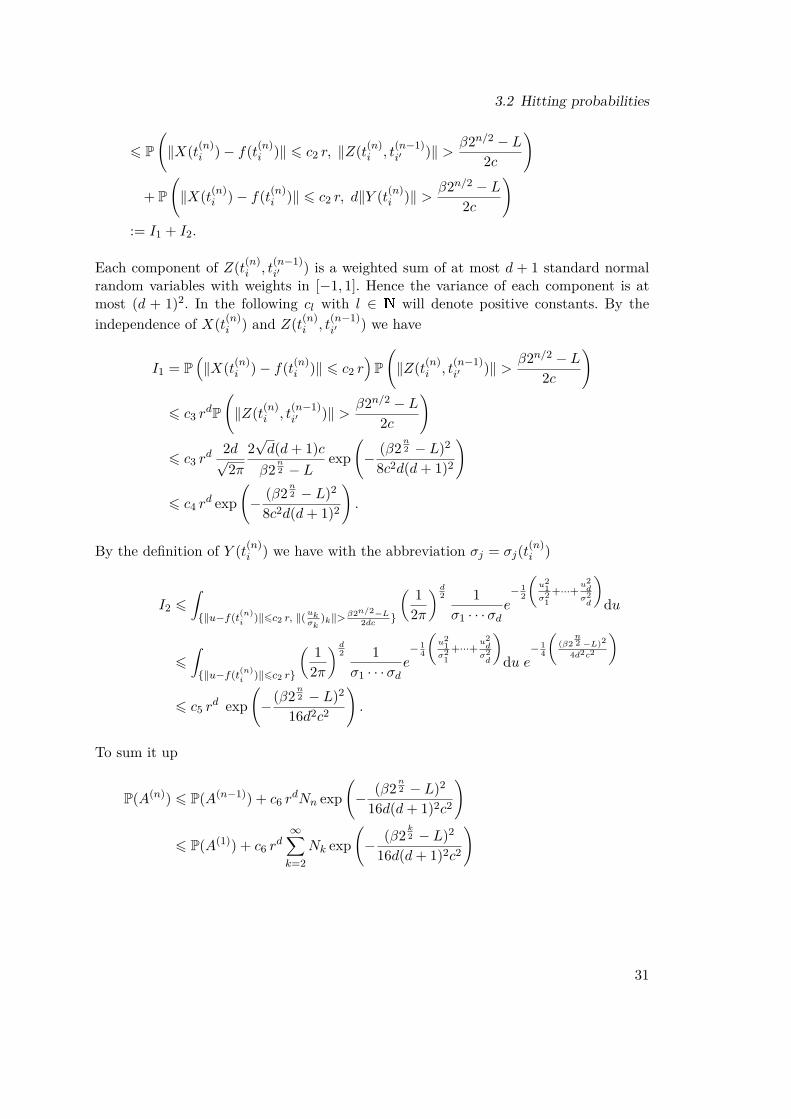
3.2 Hitting probabilities
6 P(‖X(t(n)
i )− f(t(n)i )‖ 6 c2 r, ‖Z(t(n)
i , t(n−1)i′ )‖ > β2n/2 − L
2c
)
+ P(‖X(t(n)
i )− f(t(n)i )‖ 6 c2 r, d‖Y (t(n)
i )‖ > β2n/2 − L2c
):= I1 + I2.
Each component of Z(t(n)i , t
(n−1)i′ ) is a weighted sum of at most d + 1 standard normal
random variables with weights in [−1, 1]. Hence the variance of each component is atmost (d + 1)2. In the following cl with l ∈ N will denote positive constants. By theindependence of X(t(n)
i ) and Z(t(n)i , t
(n−1)i′ ) we have
I1 = P(‖X(t(n)
i )− f(t(n)i )‖ 6 c2 r
)P(‖Z(t(n)
i , t(n−1)i′ )‖ > β2n/2 − L
2c
)
6 c3 rdP(‖Z(t(n)
i , t(n−1)i′ )‖ > β2n/2 − L
2c
)
6 c3 rd 2d√
2π2√d(d+ 1)cβ2
n2 − L
exp(− (β2
n2 − L)2
8c2d(d+ 1)2
)
6 c4 rd exp
(− (β2
n2 − L)2
8c2d(d+ 1)2
).
By the definition of Y (t(n)i ) we have with the abbreviation σj = σj(t(n)
i )
I2 6∫‖u−f(t(n)
i )‖6c2 r, ‖(ukσk
)k‖>β2n/2−L2dc
( 12π
) d2 1σ1 · · ·σd
e− 1
2
(u2
1σ2
1+···+
u2dσ2d
)du
6∫‖u−f(t(n)
i )‖6c2 r
( 12π
) d2 1σ1 · · ·σd
e− 1
4
(u2
1σ2
1+···+
u2dσ2d
)du e
− 14
((β2
n2 −L)2
4d2c2
)
6 c5 rd exp
(−(β2
n2 − L)2
16d2c2
).
To sum it up
P(A(n)) 6 P(A(n−1)) + c6 rdNn exp
(− (β2
n2 − L)2
16d(d+ 1)2c2
)
6 P(A(1)) + c6 rd∞∑k=2
Nk exp(− (β2
k2 − L)2
16d(d+ 1)2c2
)
31

3 On a related Gaussian process
6 c7rd + c6 r
d∞∑k=2
c1 exp(Q2k+1 − (β2
k2 − L)2
16d(d+ 1)2c2
).
We choose β > max(c, L/2) such that β2
16d(d+1)2c2 > 2Q. Then the sum converges andthe lemma follows by (3.17).
32
4 Asymptotic normality
This chapter presents the main results for the spectral calibration method. We proofasymptotic normality for the estimators of the volatility, the drift, the intensity andfor pointwise estimators of the jump density. The joint asymptotic distribution of theseestimators is derived. As it turns out the asymptotic behavior is different in the mildlyill–posed case of volatility zero and in the severely ill–posed case of positive volatility. Inthe mildly ill–posed case the noise grows polynomially in the frequencies while it growsexponentially in the severely ill–posed case. Through the exponential growth, the noise atthe cut–off frequency is predominant in the stochastic error. Then the noise is focused inthe spectral domain and unfocused in the spatial domain. For the mildly ill–posed case itis the other way around. Then the noise is more evenly distributed among the frequenciesbut concentrated in the spatial domain. For example, the asymptotic variance depends inthe mildly ill–posed case locally on the noise of the observations, whereas for the severelyill–posed case this dependence is global. The asymptotic normality results are used toconstruct confidence intervals and joint confidence sets in Chapter 6. In Section 4.1, wepresent the asymptotic normality results. They are discussed in Section 4.2. The proofsare deferred to Section 4.3.
4.1 Main results
The starting point of the error analysis is the decomposition (2.29) into the approxima-tion error and the stochastic error. The approximation error is deterministic and onlythe stochastic error can be expected to converge with appropriate scaling to a normalrandom variable. It is common practice to resolve this problem by undersmoothing,which means that the tuning parameter is chosen such that the approximation error be-comes asymptotically negligible. For the undersmoothing the cut–off value has to growfast enough. To obtain the exact undersmoothing conditions we first divide the orderof magnitude of the stochastic error by the order of magnitude of the approximationerror both in terms of εn and Un. Then we require that the quotient tends to infin-ity. This leads to the condition εnU
(2s+5)/2n → ∞ in the case of volatility zero and to
εnUs+1n exp(Tσ2U2
n/2) → ∞ in the case of positive volatility. Since the approximationerrors are negligible by these conditions, we will focus in the following on the stochasticerrors.In the theorems, we control the supremum of Ln,U and thus the remainder termRn,U by the conditions εnU2
n
√log(Un) → 0 and εnU
2n exp(Tσ2U2
n/2) → 0 for σ = 0and σ > 0, respectively. Then the asymptotic distribution of the stochastic errors∫ 10 ∆ψn(Uu)w(u)du is governed by the linearized stochastic errors
∫ 10 Ln,U (u)w(u)du and
33
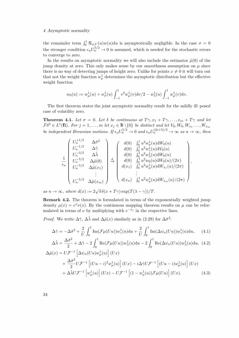
4 Asymptotic normality
the remainder term∫ 1
0 Rn,U (u)w(u)du is asymptotically negligible. In the case σ = 0the stronger condition εnU5/2
n → 0 is assumed, which is needed for the stochastic errorsto converge to zero.In the results on asymptotic normality we will also include the estimator µ(0) of the
jump density at zero. This only makes sense by our smoothness assumption on µ sincethere is no way of detecting jumps of height zero. Unlike for points x 6= 0 it will turn outthat not the weight function w1
µ determines the asymptotic distribution but the effectiveweight function
w0(u) := w1µ(u) + w1
σ(u)∫ 1
−1v2w1
µ(v)dv/2− w1λ(u)
∫ 1
−1w1µ(v)dv.
The first theorem states the joint asymptotic normality result for the mildly ill–posedcase of volatility zero.
Theorem 4.1. Let σ = 0. Let δ be continuous at Tγ, x1 + Tγ, . . . , xm + Tγ and letFδ2 ∈ L1(R). For j = 1, . . . ,m let xj ∈ R \0 be distinct and let V0,W0,Wx1 . . . ,Wxm
be independent Brownian motions. If εnU5/2n → 0 and εnU (2s+5)/2
n →∞ as n→∞, then
1εn
U+1/2n ∆σ2
U−1/2n ∆γ
U−3/2n ∆λ
U−5/2n ∆µ(0)
U−5/2n ∆µ(x1)
...U−5/2n ∆µ(xm)
d−→
d(0)∫ 1
0 u2w1
σ(u)dW0(u)d(0)
∫ 10 u
2w1γ(u)dV0(u)
d(0)∫ 1
0 u2w1
λ(u)dW0(u)d(0)
∫ 10 u
2w0(u)dW0(u)/(2π)d(x1)
∫ 10 u
2w1µ(u)dWx1(u)/(2π)
...d(xn)
∫ 10 u
2w1µ(u)dWxm(u)/(2π)
,
as n→∞, where d(x) := 2√πδ(x+ Tγ) exp(T (λ− γ))/T .
Remark 4.2. The theorem is formulated in terms of the exponentially weighted jumpdensity µ(x) = exν(x). By the continuous mapping theorem results on µ can be refor-mulated in terms of ν by multiplying with e−xj in the respective lines.
Proof. We write ∆γ, ∆λ and ∆µ(x) similarly as in (2.29) for ∆σ2:
∆γ = −∆σ2 + 2U
∫ 1
0Im(Fµ(Uu))w1
γ(u)du+ 2U
∫ 1
0Im(∆ψn(Uu))w1
γ(u)du, (4.1)
∆λ = ∆σ2
2 + ∆γ − 2∫ 1
0Re(Fµ(Uu))w1
λ(u)du− 2∫ 1
0Re(∆ψn(Uu))w1
λ(u)du, (4.2)
∆µ(x) = UF−1[∆ψn(Uu)w1
µ(u)]
(Ux)
+ ∆σ2
2 UF−1[(Uu− i)2w1
µ(u)]
(Ux)− i∆γUF−1[(Uu− i)w1
µ(u)]
(Ux)
+ ∆λUF−1[w1µ(u)
](Ux)− UF−1
[(1− w1
µ(u))Fµ(Uu)]
(Ux). (4.3)
34
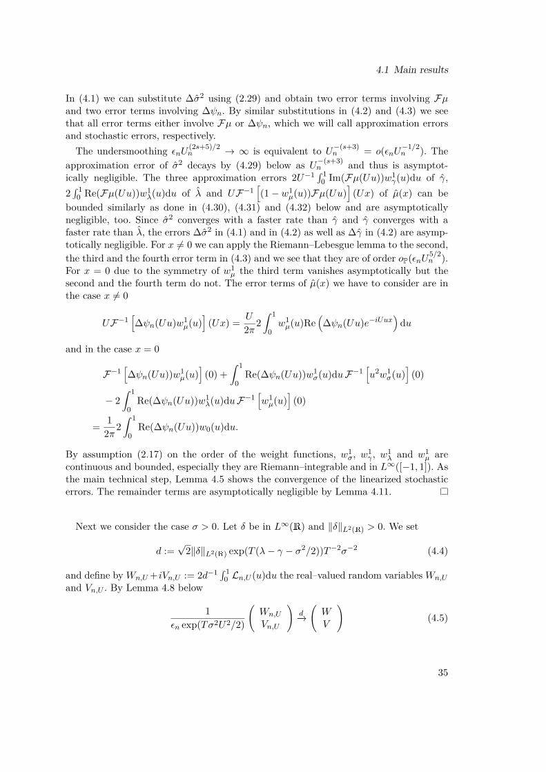
4.1 Main results
In (4.1) we can substitute ∆σ2 using (2.29) and obtain two error terms involving Fµand two error terms involving ∆ψn. By similar substitutions in (4.2) and (4.3) we seethat all error terms either involve Fµ or ∆ψn, which we will call approximation errorsand stochastic errors, respectively.The undersmoothing εnU (2s+5)/2
n → ∞ is equivalent to U−(s+3)n = o(εnU−1/2
n ). Theapproximation error of σ2 decays by (4.29) below as U−(s+3)
n and thus is asymptot-ically negligible. The three approximation errors 2U−1 ∫ 1
0 Im(Fµ(Uu))w1γ(u)du of γ,
2∫ 1
0 Re(Fµ(Uu))w1λ(u)du of λ and UF−1
[(1− w1
µ(u))Fµ(Uu)]
(Ux) of µ(x) can bebounded similarly as done in (4.30), (4.31) and (4.32) below and are asymptoticallynegligible, too. Since σ2 converges with a faster rate than γ and γ converges with afaster rate than λ, the errors ∆σ2 in (4.1) and in (4.2) as well as ∆γ in (4.2) are asymp-totically negligible. For x 6= 0 we can apply the Riemann–Lebesgue lemma to the second,the third and the fourth error term in (4.3) and we see that they are of order oP(εnU5/2
n ).For x = 0 due to the symmetry of w1
µ the third term vanishes asymptotically but thesecond and the fourth term do not. The error terms of µ(x) we have to consider are inthe case x 6= 0
UF−1[∆ψn(Uu)w1
µ(u)]
(Ux) = U
2π2∫ 1
0w1µ(u)Re
(∆ψn(Uu)e−iUux
)du
and in the case x = 0
F−1[∆ψn(Uu))w1
µ(u)]
(0) +∫ 1
0Re(∆ψn(Uu))w1
σ(u)duF−1[u2w1
σ(u)]
(0)
− 2∫ 1
0Re(∆ψn(Uu))w1
λ(u)duF−1[w1µ(u)
](0)
= 12π2
∫ 1
0Re(∆ψn(Uu))w0(u)du.
By assumption (2.17) on the order of the weight functions, w1σ, w1
γ , w1λ and w1
µ arecontinuous and bounded, especially they are Riemann–integrable and in L∞([−1, 1]). Asthe main technical step, Lemma 4.5 shows the convergence of the linearized stochasticerrors. The remainder terms are asymptotically negligible by Lemma 4.11.
Next we consider the case σ > 0. Let δ be in L∞(R) and ‖δ‖L2(R) > 0. We set
d :=√
2‖δ‖L2(R) exp(T (λ− γ − σ2/2))T−2σ−2 (4.4)
and define byWn,U +iVn,U := 2d−1 ∫ 10 Ln,U (u)du the real–valued random variablesWn,U
and Vn,U . By Lemma 4.8 below
1εn exp(Tσ2U2/2)
(Wn,U
Vn,U
)d−→(WV
)(4.5)
35
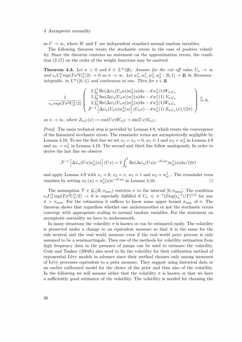
4 Asymptotic normality
as U →∞, where W and V are independent standard normal random variables.The following theorem treats the stochastic errors in the case of positive volatil-
ity. Since the theorem contains no statement on the approximation errors, the condi-tion (2.17) on the order of the weight functions may be omitted.
Theorem 4.3. Let σ > 0 and δ ∈ L∞(R). Assume for the cut–off value Un → ∞and εnU2
n exp(Tσ2U2n/2) → 0 as n → ∞. Let w1
σ, w1γ , w
1λ, w
1µ : [0, 1] → R be Riemann–
integrable, in L∞([0, 1]) and continuous at one. Then for x ∈ R
1εn exp(Tσ2U2
n/2)
2∫ 10 Re(∆ψn(Unu))w1
σ(u)du− dw1σ(1)Wn,Un
2∫ 1
0 Im(∆ψn(Unu))w1γ(u)du− dw1
γ(1) Vn,Un2∫ 1
0 Re(∆ψn(Unu))w1λ(u)du− dw1
λ(1)Wn,Un
F−1[∆ψn(Unu)w1
µ(u)]
(Unx)− dw1µ(1) Zn,Un(x)/(2π)
P−→ 0,
as n→∞, where Zn,U (x) := cos(Ux)Wn,U + sin(Ux)Vn,U .
Proof. The main technical step is provided by Lemma 4.9, which treats the convergenceof the linearized stochastic errors. The remainder terms are asymptotically negligible byLemma 4.10. To see the first line we set x1 = x2 = 0, w1 ≡ 1 and w2 = w1
σ in Lemma 4.9and wU = w1
σ in Lemma 4.10. The second and third line follow analogously. In order toderive the last line we observe
F−1[∆ψn(Uu)w1
µ(u)]
(Ux) = 2∫ 1
0Re(∆ψn(Uu)e−iUux)w1
µ(u)du/(2π)
and apply Lemma 4.9 with x1 = 0, x2 = x, w1 ≡ 1 and w2 = w1µ, . The remainder term
vanishes by setting wU (u) = w1µ(u)e−iUux in Lemma 4.10.
The assumption T ∈ Gs(R, σmax) restricts σ to the interval [0, σmax]. The conditionεnU
2n exp(Tσ2U2
n/2) → 0 is especially fulfilled if Un 6 σ−1(2 log(ε−1n )/T )1/2 for any
σ > σmax. For the estimation it suffices to know some upper bound σmax of σ. Thetheorem shows that regardless whether one undersmoothes or not the stochastic errorsconverge with appropriate scaling to normal random variables. For the statement onasymptotic normality we have to undersmooth.In many situations the volatility σ is known or can be estimated easily. The volatility
is preserved under a change to an equivalent measure so that it is the same for therisk–neutral and the real–world measure even if the real–world price process is onlyassumed to be a semimartingale. Then one of the methods for volatility estimation fromhigh frequency data in the presence of jumps can be used to estimate the volatility.Cont and Tankov (2004b) also need to fix the volatility for their calibration method ofexponential Lévy models in advance since their method chooses only among measuresof Lévy processes equivalent to a prior measure. They suggest using historical data oran earlier calibrated model for the choice of the prior and thus also of the volatility.In the following we will assume either that the volatility σ is known or that we havea sufficiently good estimator of the volatility. The volatility is needed for choosing the
36
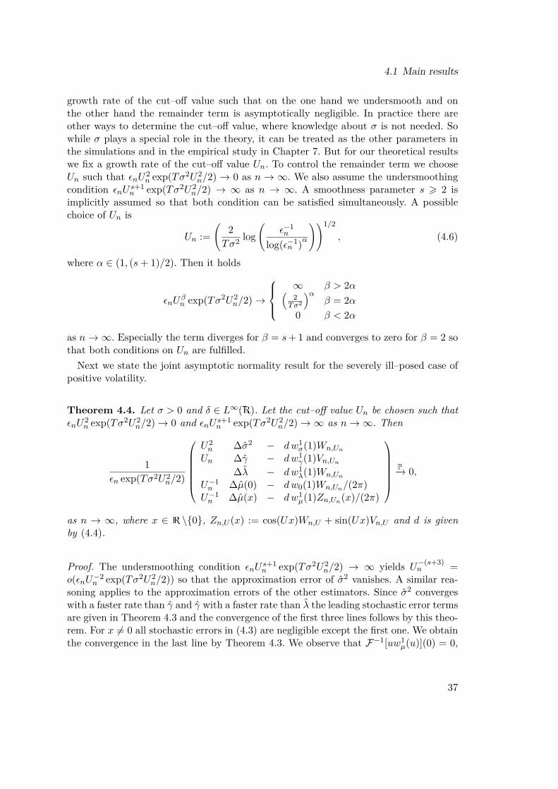
4.1 Main results
growth rate of the cut–off value such that on the one hand we undersmooth and onthe other hand the remainder term is asymptotically negligible. In practice there areother ways to determine the cut–off value, where knowledge about σ is not needed. Sowhile σ plays a special role in the theory, it can be treated as the other parameters inthe simulations and in the empirical study in Chapter 7. But for our theoretical resultswe fix a growth rate of the cut–off value Un. To control the remainder term we chooseUn such that εnU2
n exp(Tσ2U2n/2) → 0 as n → ∞. We also assume the undersmoothing
condition εnUs+1n exp(Tσ2U2
n/2) → ∞ as n → ∞. A smoothness parameter s > 2 isimplicitly assumed so that both condition can be satisfied simultaneously. A possiblechoice of Un is
Un :=(
2Tσ2 log
(ε−1n
log(ε−1n )α
))1/2
, (4.6)
where α ∈ (1, (s+ 1)/2). Then it holds
εnUβn exp(Tσ2U2
n/2)→
∞ β > 2α(2
Tσ2
)αβ = 2α
0 β < 2α
as n→∞. Especially the term diverges for β = s+ 1 and converges to zero for β = 2 sothat both conditions on Un are fulfilled.Next we state the joint asymptotic normality result for the severely ill–posed case of
positive volatility.
Theorem 4.4. Let σ > 0 and δ ∈ L∞(R). Let the cut–off value Un be chosen such thatεnU
2n exp(Tσ2U2
n/2)→ 0 and εnU s+1n exp(Tσ2U2
n/2)→∞ as n→∞. Then
1εn exp(Tσ2U2
n/2)
U2n ∆σ2 − dw1
σ(1)Wn,Un
Un ∆γ − dw1γ(1)Vn,Un
∆λ − dw1λ(1)Wn,Un
U−1n ∆µ(0) − dw0(1)Wn,Un/(2π)
U−1n ∆µ(x) − dw1
µ(1)Zn,Un(x)/(2π)
P−→ 0,
as n → ∞, where x ∈ R \0, Zn,U (x) := cos(Ux)Wn,U + sin(Ux)Vn,U and d is givenby (4.4).
Proof. The undersmoothing condition εnUs+1n exp(Tσ2U2
n/2) → ∞ yields U−(s+3)n =
o(εnU−2n exp(Tσ2U2
n/2)) so that the approximation error of σ2 vanishes. A similar rea-soning applies to the approximation errors of the other estimators. Since σ2 convergeswith a faster rate than γ and γ with a faster rate than λ the leading stochastic error termsare given in Theorem 4.3 and the convergence of the first three lines follows by this theo-rem. For x 6= 0 all stochastic errors in (4.3) are negligible except the first one. We obtainthe convergence in the last line by Theorem 4.3. We observe that F−1[uw1
µ(u)](0) = 0,
37
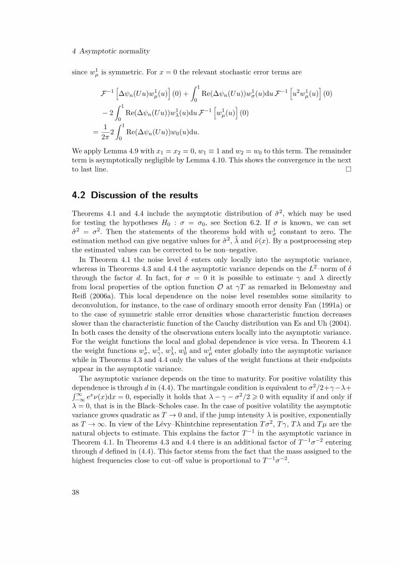
4 Asymptotic normality
since w1µ is symmetric. For x = 0 the relevant stochastic error terms are
F−1[∆ψn(Uu)w1
µ(u)]
(0) +∫ 1
0Re(∆ψn(Uu))w1
σ(u)duF−1[u2w1
µ(u)]
(0)
− 2∫ 1
0Re(∆ψn(Uu))w1
λ(u)duF−1[w1µ(u)
](0)
= 12π2
∫ 1
0Re(∆ψn(Uu))w0(u)du.
We apply Lemma 4.9 with x1 = x2 = 0, w1 ≡ 1 and w2 = w0 to this term. The remainderterm is asymptotically negligible by Lemma 4.10. This shows the convergence in the nextto last line.
4.2 Discussion of the results
Theorems 4.1 and 4.4 include the asymptotic distribution of σ2, which may be usedfor testing the hypotheses H0 : σ = σ0, see Section 6.2. If σ is known, we can setσ2 = σ2. Then the statements of the theorems hold with w1
σ constant to zero. Theestimation method can give negative values for σ2, λ and ν(x). By a postprocessing stepthe estimated values can be corrected to be non–negative.In Theorem 4.1 the noise level δ enters only locally into the asymptotic variance,
whereas in Theorems 4.3 and 4.4 the asymptotic variance depends on the L2–norm of δthrough the factor d. In fact, for σ = 0 it is possible to estimate γ and λ directlyfrom local properties of the option function O at γT as remarked in Belomestny andReiß (2006a). This local dependence on the noise level resembles some similarity todeconvolution, for instance, to the case of ordinary smooth error density Fan (1991a) orto the case of symmetric stable error densities whose characteristic function decreasesslower than the characteristic function of the Cauchy distribution van Es and Uh (2004).In both cases the density of the observations enters locally into the asymptotic variance.For the weight functions the local and global dependence is vice versa. In Theorem 4.1the weight functions w1
σ, w1γ , w1
λ, w10 and w1
µ enter globally into the asymptotic variancewhile in Theorems 4.3 and 4.4 only the values of the weight functions at their endpointsappear in the asymptotic variance.The asymptotic variance depends on the time to maturity. For positive volatility this
dependence is through d in (4.4). The martingale condition is equivalent to σ2/2+γ−λ+∫∞−∞ e
xν(x)dx = 0, especially it holds that λ− γ − σ2/2 > 0 with equality if and only ifλ = 0, that is in the Black–Scholes case. In the case of positive volatility the asymptoticvariance grows quadratic as T → 0 and, if the jump intensity λ is positive, exponentiallyas T →∞. In view of the Lévy–Khintchine representation Tσ2, Tγ, Tλ and Tµ are thenatural objects to estimate. This explains the factor T−1 in the asymptotic variance inTheorem 4.1. In Theorems 4.3 and 4.4 there is an additional factor of T−1σ−2 enteringthrough d defined in (4.4). This factor stems from the fact that the mass assigned to thehighest frequencies close to cut–off value is proportional to T−1σ−2.
38
4.3 Proof of the asymptotic normality
For w1σ(1), w1
γ(1), w1λ(1), w1
µ(1) ∈ R \0, Theorem 4.3 describes the asymptotic dis-tribution of the leading stochastic error terms of σ2, γ, λ and µ(x), x 6= 0, i.e., the otherstochastic error terms are of smaller order. Theorem 4.4 describes the asymptotic dis-tribution of the estimation errors. Both theorems are for the case of positive volatility,where the noise in the frequency domain is exponentially heteroscedastic, so that thehighest frequency, that is the cut–off frequency U , dominates the stochastic error. Thenthis cut–off frequency U can be seen in the asymptotic distribution of ∆µ through theoscillating process Zn,U . The variances in Theorems 4.3 and 4.4 converge by (4.5) and bythe definition of Zn,U (x). If one only considers the stochastic errors of σ2, γ, λ and µ(0),then the covariances converge, too. But for x 6= 0 the covariance of the stochastic errorsof µ(x) and of σ2 does not converge. The same holds for the covariance of the stochasticerrors of µ(x) and γ as well as µ(x) and λ. The phenomenon that the covariances donot convergence comes from the fact that the stochastic error centers more and moreat the cut–off frequency. The sequence of cut–off values has a crucial influence on thecovariance. For estimators of the generalized distribution function of the jump densitythis is likely to lead to a similar dependence on the sequence of cut–off values as observedin van Es and Uh (2005) for deconvolution with supersmooth errors.
4.3 Proof of the asymptotic normality
4.3.1 The linearized stochastic errors
The linearized stochastic errors are of the form∫ 1
0 fj(u)Ln,U (u)du, where fj with j =1, . . . , n are Riemann–integrable functions in L∞([0, 1]). Next we will show that theseare jointly normal distributed. Almost surely Ln,U is continuous. Thus, almost surelythe fjLn,U are Riemann–integrable and almost surely
1m
m∑k=1
fj(k/m)Ln,U (k/m)→∫ 1
0fj(u)Ln,U (u)du
as m → ∞. Let C > 0 be such that ‖fj‖∞ 6 C for all j = 1, . . . , n. For each mthe n sums are joint, centered normal random variables. For m → ∞ the covariancematrix converges by the dominated convergence theorem with the dominating functionC2 supu∈[0,1] |Ln,U (u)|2, where supu∈[0,1] |Ln,U (u)|2 is an integrable random variable byProposition 3.3. Thus, the characteristic function converges pointwise. By Lévy’s con-tinuity theorem this shows that the sums convergence jointly in distribution to normalrandom variables. So
∫ 10 fj(u)Ln,U (u)du are jointly normal distributed.
For a fixed cut–off value U the linearized stochastic errors are jointly normal dis-tributed. So the natural question is whether the appropriately scaled covariance matrixconverges for U →∞.
39
4 Asymptotic normality
Let wj , wk : [0, 1]→ R be Riemann–integrable functions in L∞([0, 1]). It holds
T
∫ 1
0wj(u)Ln,U (u)e−iUuxjdu
= εnU2e−T (σ2/2+γ−λ)
∫ 1
0fU (u)
∫ ∞−∞
eiUu(x−θj)+Tσ2U2u2/2δ(x)dW (x)du,
wherefU (u) := wj(u)(−u2 + iu/U)
exp(TFµ(Uu)) (4.7)
and θj := xj + Tσ2 + Tγ. We define analogously
gU (u) := wk(u)(−u2 + iu/U)exp(TFµ(Uu)) (4.8)
and θk := xk + Tσ2 + Tγ. We extend fU and gU by zero outside the interval [0, 1].
Since E[supu∈[−1,1] |Ln,U (u)|2
]< ∞, we may apply Fubini’s theorem and then we
apply the Itô isometry to obtain
T 2e2T (σ2/2+γ−λ)E[∫ 1
0wj(u)Ln,U (u)e−iUuxjdu
∫ 1
0wk(v)Ln,U (v)e−iUvxkdv
]
= ε2nU4∫ 1
0
∫ 1
0
∫ ∞−∞
fU (u)eiUu(x−θj)+Tσ2U2u2/2
gU (v)eiUv(x−θk)+Tσ2U2v2/2δ(x)2dxdudv. (4.9)
To separate real and imaginary part we will also need
T 2e2T (σ2/2+γ−λ)E[∫ 1
0wj(u)Ln,U (u)e−iUuxjdu
∫ 1
0wk(v)Ln,U (v)e−iUvxkdv
]= ε2nU
4∫ 1
0
∫ 1
0
∫ ∞−∞
fU (u)eiUu(x−θj)+Tσ2U2u2/2
gU (v)eiUv(x−θk)+Tσ2U2v2/2δ(x)2dxdudv. (4.10)
Lemma 4.5. Let σ = 0. For j = 1, . . . ,m let xj ∈ R and let wj : [0, 1]→ R be Riemann–integrable functions in L∞([0, 1]). Let δ be continuous at x1 +Tγ, x2 +Tγ, . . . , xm +Tγand let Fδ2 ∈ L1(R). Let Wx1 , . . . ,Wxm , Vx1 , . . . , Vxm be Brownian motions. If xj = xklet Wxj = Wxk and Vxj = Vxk otherwise let the Brownian motions be distinct. Let theset Wx1 , . . . ,Wxm , Vx1 , . . . , Vxm consist of independent Brownian motions. Then
1εnU3/2
∫ 1
0wj(u)Ln,U (u)e−iUuxjdu
40
4.3 Proof of the asymptotic normality
converge jointly in distribution to√πδ(xj + Tγ)
T exp(T (γ − λ))
(∫ 1
0u2wj(u)dWxj (u) + i
∫ 1
0u2wj(u)dVxj (u)
)as U →∞.
Proof. We will first consider the case xj = xk. We have seen that
T 2e2T (γ−λ)E[∫ 1
0wj(u)Ln,U (u)e−iUuxjdu
∫ 1
0wk(v)Ln,U (v)e−iUvxjdv
]
= ε2nU4∫ ∞−∞FfU (U(x− θj))FgU (U(x− θj))δ(x)2dx,
where fU and gU are defined as in (4.7) and (4.8), respectively, and θj = xj + Tγ,
= ε2nU3∫ ∞−∞FfU (y)FgU (y)δ(y/U + θj)2dy.
We notice that Fδ2 ∈ L1(R) implies δ2 ∈ L∞(R) and we obtain by the Plancherelidentity
= 2πε2nU3∫ 1
0fU (u)(gU (v) ∗ F−1(δ(y/U + θj)2)(v))(u)du, (4.11)
since the support of fU is [0, 1]. Because we are only interested in the limit U →∞, wemay assume U > 1. By the Riemann–Lebesgue lemma Fµ(u) tends to zero as |u| → ∞.The factor fU (u) converges for each u ∈ [0, 1] to −u2wj(u) as U →∞ and the functionsare dominated by a constant independent of U . In order to apply dominated convergenceit suffices that the second factor is dominated by a constant independent of U andconverges stochastically with respect to the Lebesgue measure on R.
(gU (v) ∗ F−1(δ(y/U + θj)2)(v))(u) =∫ ∞−∞
gU (u− v)F−1(δ(y + θj)2)(Uv)Udv
By assumption Fδ2 lies in L1(R) and so does F−1(δ(y + θj)2). A dominating constantis√
2‖wk‖∞ exp(T‖Fµ‖∞) ‖F−1(δ(y + θj)2)‖L1(R). It holds∫ ∞−∞F−1(δ(y + θj)2)(Uv)Udv =
∫ ∞−∞F−1(δ(y + θj)2)(v)dv
= FF−1(δ(y + θj)2)(0) = δ(θj)2. (4.12)
δU (v) := F−1(δ(y + θj)2)(Uv)U is the multiple of what is called approximate identityor nascent delta function (Grafakos, 2004, Definition 1.2.15). For h ∈ L1(R) and anapproximate identity δn we have that h ∗ δn converges to h in L1(R) as n → ∞. Thus,(−v2wk(v)1[0,1](v))∗δU (v)(u) converges to −u2wk(u)1[0,1](u)δ(θj)2 for U →∞ in L1(R)
41
4 Asymptotic normality
(Grafakos, 2004, p. 28) and in particular stochastically (Klenke, 2007, Definition 6.2).If u 6= 0, then there is a neighborhood of u where gU (u) + u2wk(u)1[0,1](u) convergesuniformly to zero. (gU (v)+v2wk(v)1[0,1](v))∗δU (v)(u) converges almost surely and in par-ticular stochastically to zero. Thus, gU (v)∗δU (v)(u) converges to −u2wk(u)1[0,1](u)δ(θj)2
stochastically with respect to the Lebesgue measure on R.
We obtain under the limit U →∞ by the dominated convergence theorem
limU→∞
1ε2nU
3E[∫ 1
0wj(u)Ln,U (u)e−iUuxjdu
∫ 1
0wk(v)Ln,U (v)e−iUvxjdv
]
= 2πδ(θj)2
T 2 exp(2T (γ − λ))
∫ ∞−∞
(−u2wj(u)1[0,1](u)
) (−u2wk(u)1[0,1](u)
)du
= 2πδ(θj)2
T 2 exp(2T (γ − λ))
∫ 1
0u4wj(u)wk(u)du. (4.13)
Without taking the complex conjugate in (4.11) we obtain
T 2e2T (γ−λ)E[∫ 1
0wj(u)Ln,U (u)e−iUuxjdu
∫ 1
0wk(v)Ln,U (v)e−iUvxjdv
]= 2π
∫ ∞−∞
fU (u)(gU (−v) ∗ F−1(δ(y/U + θj)2)(v))(u)du.
The same argumentation as before leads to
limU→∞
E[∫ 1
0wj(u)Ln,U (u)e−iUuxjdu
∫ 1
0wk(v)Ln,U (v)e−iUvxjdv
]= 2πδ(θj)2
T 2 exp(2T (γ − λ))
∫ ∞−∞
(−u2wj(u)1[0,1](u)
) (−u2wk(−u)1[0,1](−u)
)du
= 0. (4.14)
We combine (4.13) and (4.14) to obtain
limU→∞
1ε2nU
3E[Re∫ 1
0
wj(u)Ln,U (u)exp(iUuxj)
du Re∫ 1
0
wk(u)Ln,U (u)exp(iUuxj)
dv]
= limU→∞
1ε2nU
3E[Im∫ 1
0
wj(u)Ln,U (u)exp(iUuxj)
du Im∫ 1
0
wk(u)Ln,U (u)exp(iUuxj)
dv]
= πδ(θj)2
T 2 exp(2T (γ − λ))
∫ 1
0u4wj(u)wk(u)du.
From (4.13) and (4.14) it also follows that the covariance between real and imaginarypart vanishes asymptotically.
In the case xj 6= xk, we have to show that the covariance vanishes asymptotically.Without loss of generality we assume xj < xk. We define θ := (θj + θk)/2, yielding
42
4.3 Proof of the asymptotic normality
θj < θ < θk. We have
T 2e2T (γ−λ)
ε2nU3 E
[∫ 1
0wj(u)Ln,U (u)e−iUuxjdu
∫ 1
0wk(v)Ln,U (v)e−iUvxkdv
]
=∫ ∞−∞FfU (U(x− θj))FgU (U(x− θk))δ(x)2Udx
=∫ ∞−∞FfU (y + U(θ − θj))FgU (y + U(θ − θk))δ(y/U + θ)2dy.
By the Plancherel identity and by the dominated convergence theorem
FfU → F(−u2wj(u)
)and FgU → F
(−u2wk(u)
)in L2(R) for U → ∞ and especially the L2(R) norms converge. From the assumptionFδ2 ∈ L1(R) follows that δ2 ∈ L∞(R). By the Cauchy–Schwarz inequality
limU→∞
∣∣∣∣∫ 0
−∞FfU (y + U(θ − θj))FgU (y + U(θ − θk))δ(y/U + θ)2dy
∣∣∣∣6 lim
U→∞‖δ‖2∞ ‖FfU‖L2(R)
(∫ U(θ−θk)
−∞|FgU (y)|2 dy
)1/2
= 0.
A similar calculation shows that the integral over (0,∞) converges to zero and conse-quently
limU→∞
T 2e2T (γ−λ)
ε2nU3 E
[∫ 1
0
wj(u)Ln,U (u)exp(iUuxj)
du∫ 1
0
wk(v)Ln,U (v)exp(iUvxk)
dv]
= 0.
The same way follows
limU→∞
T 2e2T (γ−λ)
ε2nU3 E
[∫ 1
0
wj(u)Ln,U (u)exp(iUuxj)
du∫ 1
0
wk(v)Ln,U (v)exp(iUvxk)
dv]
= 0.
The 1/(εnU3/2)∫ 1
0 wj(u)Ln,U (u)e−iUuxjdu are centered normal random variables andtheir covariance matrix converges to the covariance matrix of the claimed limit. Thus,the characteristic function converges pointwise. By Lévy’s continuity theorem this showsthe convergence in distribution.
Lemma 4.6. Let σ > 0 and δ ∈ L∞(R). Let wU , wU ∈ L∞([0, 1],C) be Riemann–integrable and let there be a constant C > 0 such that for all U > 1 ‖wU‖∞, ‖wU‖∞ 6 C.Let there be a, a : [1,∞)→ C such that the condition
limη→0
supU>1
supu∈[1−η/U,1]
|wU (u)− a(U)| = 0 (4.15)
43

4 Asymptotic normality
and the corresponding condition for wU and a hold. Then
limU→∞
1ε2n exp(Tσ2U2)E
[∫ 1
0wU (u)Ln,U (u)du
∫ 1
0wU (v)Ln,U (v)dv
]= 0,
limU→∞
( 1ε2n exp(Tσ2U2)E
[∫ 1
0wU (u)Ln,U (u)du
∫ 1
0wU (v)Ln,U (v)dv
]
−a(U)a(U)
∫∞−∞ δ(y)2dy
exp(2T (σ2/2 + γ − λ))T 4σ4
)= 0.
Remark 4.7. Obviously a(U) := wU (1) is the only possible definition. Thus, a describesthe dependence of wU on U at one.
Proof. We notice that (4.9) applies to the complex–valued functions and yields for wj :=wU and wk := wU with the definitions (4.7) and (4.8) of fU and gU , respectively, andwith θ := Tσ2 + Tγ
T 2e2T (σ2/2+γ−λ)E[∫ 1
0wU (u)Ln,U (u)du
∫ 1
0wU (v)Ln,U (v)dv
]
= ε2nU4∫ ∞−∞F(fU (u)eTσ2U2u2/2)(U(x− θ))F(gU (v)eTσ2U2v2/2)(U(x− θ))δ(x)2dx,
= 2πε2nU3∫ ∞−∞
fU (u)eTσ2U2u2/2(gU (v)eTσ2U2v2/2 ∗ F−1(δ(y/U + θ)2)(v)
)(u)du
= 2πε2nU4∫ 1
0
∫ 1
0fU (u)gU (v)F−1(δ(y + θ)2)(U(u− v))eTσ2U2(u2+v2)/2dudv. (4.16)
For all η > 0 we have
limU→∞
Tσ2U2e−Tσ2U2/2
∫ 1
1−η/UueTσ
2U2u2/2du
= limU→∞
e−Tσ2U2/2
[eTσ
2U2u2/2]1
1−η/U= 1− lim
U→∞e−Tσ
2Uη+Tσ2η2/2 = 1. (4.17)
For the product of two such sequences we obtain for all η > 0
limU→∞
T 2σ4U4e−Tσ2U2
∫ 1
1−η/U
∫ 1
1−η/UuveTσ
2U2(u2+v2)/2dudv = 1. (4.18)
Likewise
limU→∞
T 2σ4U4e−Tσ2U2
∫ 1
0
∫ 1
0uveTσ
2U2(u2+v2)/2dudv = 1 (4.19)
44
4.3 Proof of the asymptotic normality
holds. We scale the integral in (4.16) appropriately:
limU→∞
(T 2σ4U4e−Tσ
2U2∫ 1
0
∫ 1
0fU (u)gU (v) (4.20)
F−1(δ(y + θ)2)(U(u− v))eTσ2U2(u2+v2)/2dudv − a(U)a(U) 12π
∫ ∞−∞
δ(y)2dy)
= limU→∞
(T 2σ4U4e−Tσ
2U2∫ 1
0
∫ 1
0uveTσ
2U2(u2+v2)/2 (4.21)
F−1(δ(y + θ)2)(U(u− v))fU (u)gU (v)/(uv)dudv − a(U)a(U) 12π
∫ ∞−∞
δ(y)2dy)
We recall that in the Gaussian white noise model we assumed δ to be in L2(R). SinceF−1(δ(y + θ)2)(U(u− v))fU (u)gU (v)/(uv) is bounded in L∞([0, 1]2) independently of Ufor U > 1 and since the difference between (4.19) and (4.18) is zero, only the integralover [1− η/U, 1]2 contributes to the limit. For all η > 0 the limit equals
= limU→∞
(T 2σ4U4e−Tσ
2U2∫ 1
1−η/U
∫ 1
1−η/UuveTσ
2U2(u2+v2)/2 (4.22)
F−1(δ(y + θ)2)(U(u− v))fU (u)gU (v)/(uv)dvdu− a(U)a(U) 12π
∫ ∞−∞
δ(y)2dy)
= 0,
which can be seen the following way. F−1(δ(y + θ)2) is continuous and |U(u − v)| 6 ηfor all u, v ∈ [1− η/U, 1]. So by choosing η small enough F−1(δ(y + θ)2)(U(u− v)) getsarbitrarily close to F−1(δ(y + θ)2)(0) = (1/2π)
∫∞−∞ δ(y)2dy. By (4.15), wU (u) tends to
a(U) and wU (v) tends to a(U) for η tending to zero. By choosing U , large the factor(−u + i/U)/ exp(TFµ(Uu)) gets close to minus one for all u ∈ [1 − η/U, 1]. Thus,for small η and large U the term fU (u)gU (v)/(uv) is close to a(U)a(U) for all u, v ∈[1− η/U, 1].
Rescaling (4.16) and taking the limit U →∞ leads to
limU→∞
( 1ε2n exp(Tσ2U2)E
[∫ 1
0wU (u)Ln,U (u)du
∫ 1
0wU (v)Ln,U (v)dv
]
−a(U)a(U)
∫∞−∞ δ(y)2dy
exp(2T (σ2/2 + γ − λ))T 4σ4
)= lim
U→∞
( 2πU4 exp(−Tσ2U2)T 2 exp(2T (σ2/2 + γ − λ))
∫ 1
0
∫ 1
0fU (u)gU (v)
F−1(δ(y + θ0)2)(U(u− v))eTσ2U2(u2+v2)/2dudv
− 2πexp(2T (σ2/2 + γ − λ))
a(U)a(U)T 4σ42π
∫ ∞−∞
δ(y)2dy)
= 0, (4.23)
45
4 Asymptotic normality
where we used that (4.20) is zero. By (4.10) with y = U(x− θ) we have
T 2e2T (σ2/2+γ−λ)E[∫ 1
0wU (u)Ln,U (u)du
∫ 1
0wU (v)Ln,U (v)dv
]= ε2nU
3∫ ∞−∞F(fU (u)eTσ2U2u2/2)(y)F(gU (−v)eTσ2U2v2/2)(y)δ(y/U + θ)2dy
= 2πε2nU3∫ ∞−∞
fU (u)eTσ2U2u2/2(gU (−v)eTσ2U2v2/2 ∗ F−1(δ(y/U + θ)2)(v)
)(u)du
= 2πε2nU4∫ 1
0
∫ 0
−1fU (u)gU (−v)F−1(δ(y + θ)2)(U(u− v))eTσ2U2(u2+v2)/2dvdu
= 2πε2nU4∫ 1
0
∫ 1
0uveTσ
2U2(u2+v2)/2F−1(δ(y + θ)2)(−U(u+ v))fU (u)gU (v)uv
dvdu.
Rescaling as in (4.23) leads to
limU→∞
1ε2n exp(Tσ2U2)E
[∫ 1
0wU (u)Ln,U (u)du
∫ 1
0wU (v)Ln,U (v)dv
]= lim
U→∞
2πU4 exp(−Tσ2U2)T 2 exp(2T (σ2/2 + γ − λ))
∫ 1
0
∫ 1
0uveTσ
2U2(u2+v2)/2
F−1(δ(y + θ)2)(−U(u+ v))fU (u)gU (v)/(uv)dudv = 0, (4.24)
since F−1(δ(y + θ)2)(u)→ 0 for |u| → ∞.
Lemma 4.8. Let σ > 0 and δ ∈ L∞(R). Let x0 ∈ R and for j = 1, . . . , n let wj :[0, 1]→ R be continuous at one, Riemann–integrable and in L∞([0, 1]). Then
1εn exp(Tσ2U2/2)
∫ 1
0wj(u)Ln,U (u)e−iUux0du
converge jointly in distribution to
‖δ‖L2(R)wj(1)√
2 exp(T (σ2/2 + γ − λ))T 2σ2 (W + iV )
as U →∞, where W and V are independent standard normal random variables.
Proof. This is a consequence of Lemma 4.6. We define wU (u) := wj(u)/ exp(iUux0) andwU (u) := wk(u)/ exp(iUux0). Further we set a(U) := wj(1)/ exp(iUx0) and a(U) :=wk(1)/ exp(iUx0). Then we apply Lemma 4.6. Condition (4.15) is satisfied since wjand wk are continuous at one and since exp(−iUux0) = exp(−iUx0) exp(iU(1 − u)x0),where U(1 − u) 6 η for u ∈ [1 − η/U, 1]. We note that a(U)a(U) = wj(1)wk(1) is real.By Lemma 4.6 the covariances converge to the covariances of the claimed limit. Theconvergence in distribution follows by Lévy’s continuity theorem.
46

4.3 Proof of the asymptotic normality
Lemma 4.9. Let σ > 0 and δ ∈ L∞(R). Let w1, w2 : [0, 1]→ R be Riemann–integrable,in L∞([0, 1]) and continuous at one. Let x1, x2 ∈ R and denote x2 − x1 by ϕ. Then
1εneTσ
2U2/2
(w1(1)
∫ 1
0
w2(u)Ln,U (u)eiUux2
du− w2(1)eiUϕ
∫ 1
0
w1(u)Ln,U (u)eiUux1
du)
P−→ 0,
as U →∞.
Proof. The proof relies on Lemma 4.6. We define
wU (u) := w1(1)w2(u)exp(iUux2) −
w2(1)w1(u)exp(iUϕ) exp(iUux1) .
wU (u) fulfills condition (4.15) with a(U) = 0 for all U > 1. Lemma 4.6 yields
limU→∞
1ε2n exp(Tσ2U2)E
[∣∣∣∣∫ 1
0wU (u)Ln,U (u)du
∣∣∣∣2]
= 0
and the statement follows by Lévy’s continuity theorem.
4.3.2 The remainder term
In this section, we show that the contribution of the remainder term to the estima-tion vanishes asymptotically. We recall that the remainder term Rn,U depends on thecharacteristic triplet.
Lemma 4.10. Let σ0 > 0. Let wU ∈ L∞([0, 1],C) be Riemann–integrable and let therebe a constant C > 0 such that ‖wU‖∞ 6 C for all U > 1. If εnU2
n exp(Tσ20U
2n/2)→ 0 as
n→∞, then for all characteristic triplets with σ 6 σ0
1εn exp(Tσ2
0U2n/2)
∫ 1
0wUn(u)Rn,Un(u)du P−→ 0, as n→∞.
Proof. By the identity Rn,U (u) = (1/T ) log>κU (u)(1+TLn,U (u))−Ln,U (u) with κU (u) 61/2, we have to show that with the abbreviation U = Un
1εn exp(Tσ2
0U2/2)
∫ 1
0wU (u)
(log>κU (u)(1 + TLn,U (u))− TLn,U (u)
)du (4.25)
converges in probability to zero.For z ∈ C holds log(1 + z) − z = O(|z|2) as |z| → 0. We define g by g(z) := (log(1 +
z) − z)/|z|2 for z 6= 0 and g(0) := 0. There are M and η > 0 such that |g(z)| 6 Mfor all |z| 6 η. We may assume that η 6 1/2. If the logarithm in the definition of g isreplaced by the trimmed logarithm log>κ with κ ∈ (0, 1/2] then g remains unchangedfor |z| 6 1/2. Thus, the statement holds uniformly for all gκ(z) := (log>κ(1+z)−z)/|z|2with κ ∈ (0, 1/2].
47
4 Asymptotic normality
By Proposition 3.3 we have supu∈[−1,1] |Ln,U (u)| P−→ 0. Let τ > 0 be given. Eventuallywe have
P(∃u ∈ [−1, 1] : | log>κU (u)(1 + TLn,U (u))− TLn,U (u)| > MT 2|Ln,U (u)|2
)6 P
(T supu∈[−1,1]
|Ln,U (u)| > η
)< τ.
Except on a set with probability less than τ we have eventually
1εn exp(Tσ2
0U2/2)
∣∣∣∣∫ 1
0wU (u)
(log>κU (u)(1 + TLn,U (u))− TLn,U (u)
)du∣∣∣∣
6MT 2
εn exp(Tσ20U
2/2)
∫ 1
0|wU (u)Ln,U (u)2|du. (4.26)
Hence (4.25) converges in probability to zero if (4.26) converges in probability to zero.The convergence
1εn exp(Tσ2
0U2/2)
∫ 1
0|wU (u)Ln,U (u)2|du→ 0
holds even in L1 since
1εn exp(Tσ2
0U2/2)
E[∫ 1
0|wU (u)Ln,U (u)2|du
](4.27)
6C
εn exp(Tσ20U
2/2)E[∫ 1
0|Ln,U (u)2|du
]6
C
εn exp(Tσ20U
2/2)∫ 1
0
∣∣∣∣ εn iUu(1 + iUu)T (1 + iUu(1 + iUu)FO(Uu))
∣∣∣∣2 E[∣∣∣∣∫ ∞−∞
eiUuxδ(x)dW (x)∣∣∣∣2]
du
6C
εn exp(Tσ20U
2/2)
∫ 1
0
ε2n(U2 + U4)u exp(Tσ2U2u2)‖δ‖2L2(R)T 2 exp(2T (σ2/2 + γ − λ)− 2T‖Fµ‖∞)du, (4.28)
for σ = 0 this converges to zero and for σ > 0 we further calculate,
=Cεn(1 + U2)‖δ‖2L2(R)
∫ 10 2Tσ2U2u exp(Tσ2U2u2)du
exp(Tσ20U
2/2)2T 3σ2 exp(2T (σ2/2 + γ − λ)− 2T‖Fµ‖∞)
=Cεn(1 + U2)‖δ‖2L2(R)(exp(Tσ2U2)− 1)
exp(Tσ20U
2/2)2T 3σ2 exp(2T (σ2/2 + γ − λ)− 2T‖Fµ‖∞)
6C‖δ‖2L2(R)εn(1 + U2)(exp(Tσ2
0U2/2))
2T 3σ2 exp(2T (σ2/2 + γ − λ)− 2T‖Fµ‖∞) → 0
as n→∞. Thus, (4.25) converges in probability to zero.
48
4.3 Proof of the asymptotic normality
Lemma 4.11. Let wU ∈ L∞([0, 1],C) be Riemann–integrable and let there be a constantC > 0 such that ‖wU‖∞ 6 C for all U > 1. If Un → ∞ and εnU5/2
n → 0 as n → ∞,then for all characteristic triplets with σ = 0
1εnU
3/2n
∫ 1
0wUn(u)Rεn,Un(u)du P−→ 0,
as n→∞.
Proof. We follow the proof of Lemma 4.10. We have supu∈[−1,1] |Ln,U (u)| P−→ 0 by Propo-sition 3.3. We set σ0 = 0 and divide by U3/2 in (4.25) and (4.26). Then we use that(4.27) is bounded by (4.28), where we set σ0 = σ = 0 and divide by U3/2 again. Weobtain
1εnU3/2E
[∫ 1
0|wU (u)Ln,U (u)2|du
]6
Cεn (U1/2 + U5/2)‖δ‖2L2(R)T 2 exp(T (2(γ − λ)− 2‖Fµ‖∞)) → 0
as εn → 0, which implies the desired convergence.
4.3.3 The approximation errors
The approximation error can be controlled as in Belomestny and Reiß (2006a) using theorder conditions (2.17) on the weight functions. The characteristic triplet T = (σ2, γ, µ)was assumed to be contained in Gs(R, σmax), especially µ is s–times weakly differentiableand we have max06k6s ‖µ(k)‖L2(R) 6 R, ‖µ(s)‖∞ 6 R.
We use (iu)sFµ(u) = Fµ(s)(u) and the Plancherel identity to bound the approxima-tion error by ∣∣∣∣ 2
U2
∫ 1
0Re(Fµ(Uu))w1
σ(u)du∣∣∣∣ = 1
U2
∣∣∣∣∫ 1
−1Fµ(Uu)w1
σ(u)du∣∣∣∣
= 2πU2
∣∣∣∣∫ ∞−∞
µ(s)(x/U)U−1F−1(w1σ(u)/(iUu)s)(x)dx
∣∣∣∣6 U−(s+3)‖µ(s)‖∞‖F(w1
σ(u)/us)‖L1(R). (4.29)
Analogously we obtain∣∣∣∣ 2U
∫ 1
0Im(Fµ(Uu))w1
γ(u)du∣∣∣∣ 6 U−(s+2)‖µ(s)‖∞‖F(w1
γ(u)/us)‖L1(R), (4.30)∣∣∣∣2 ∫ 1
0Re(Fµ(Uu))w1
λ(u)du∣∣∣∣ 6 U−(s+1)‖µ(s)‖∞‖F(w1
λ(u)/us)‖L1(R). (4.31)
49

4 Asymptotic normality
The last error term in (4.3) can be bounded by∣∣∣UF−1[(1− w1
µ(u))Fµ(Uu)]
(Ux)∣∣∣ = U
2π
∣∣∣∣∫ ∞−∞
(1− w1µ(u))Fµ(Uu)e−iUuxdu
∣∣∣∣= 1
2πU s−1
∣∣∣∣∣∫ ∞−∞
1− w1µ(u)
useiUuxFµ(s)(Uu)du
∣∣∣∣∣= U−s
∣∣∣∣∣∣∫ ∞−∞F−1
(1− w1
µ(u)us
eiUux
)(y)µ(s)
(y
U
)dy
∣∣∣∣∣∣6‖µ(s)‖∞
2πU s
∥∥∥∥∥F(
1− w1µ(u)
us
)∥∥∥∥∥L1(R)
. (4.32)
50
5 Uniformity with respect to the underlyingprobability measure
In order to obtain honest confidence sets, we have to consider asymptotic normality notonly for one single probability measure but rather over a class of probability measures.To this end, we will extend the asymptotic normality results of Chapter 4. The resultshold for each characteristic triplet T ∈ Gs(R, σmax) specified in Definition 2.4. Thespeed of convergence might depend on T . To make statements on confidence sets andon hypotheses tests it is useful to control the speed of convergence uniformly over aclass of characteristic triplets. We fix some arbitrarily slowly decreasing function h withh(u) → 0 as |u| → ∞. We will show uniform convergence for the class Hs(R, σmax)consisting of all characteristic triplets in Gs(R, σmax) satisfying the additional conditions
‖Fµ‖∞ 6 R and |Fµ(u)| 6 Rh(u), ∀u ∈ R . (5.1)
The first condition can easily be ensured by ‖µ‖L1(R) 6 R. For h(u) = |u|−1 the secondcondition can be ensured by ‖µ′‖L1(R) 6 R. For each characteristic triplet in Gs(R, σmax)the function Fµ(u) tends to zero as |u| → 0 by the Riemann–Lebesgue lemma. Especiallyfor each T ∈ Gs(R, σmax) there are h and R > 0 such that T ∈ Hs(R, σmax).In the case σ > 0 some covariances do not converge. We show uniform convergence
for the joint distribution only in such cases, where the covariances do converge. As itturns out it is also important that the covariance matrix of the limit is nondegenerate.We cover uniform convergence of σ2, γ, λ, µ(x) and of the pair (γ, λ).In Section 5.1, we describe our general approach to obtain uniform convergence with
respect to the underlying probability measure. Section 5.2 and Section 5.3 cover thespecific aspects for volatility zero and for positive volatility, respectively. Section 5.4treats uniformity in the probability measure for the remainder term.
5.1 General approach
Before we state the uniform version of our asymptotic normality results, we begin withsome definitions. A sequence of random variables Xn converges to X in total variationif
supB|P(Xn ∈ B)− P(X ∈ B)| → 0
51
5 Uniformity with respect to the underlying probability measure
as n→∞, where the supremum is taken over all measurable sets B. For sequences Xϑ,n,ϑ ∈ Θ, we say that they converge to X in total variation uniformly over Θ if
supϑ∈Θ
supB|P(Xϑ,n ∈ B)− P(X ∈ B)| → 0
as n→∞. The extension of convergence in total variation to convergence in total vari-ation uniformly over Θ is canonic. How to define convergence in distribution uniformlyover Θ is less clear. By the Portmanteau theorem there are a number of equivalentdefinitions of convergence in distribution. One definition is that a sequence of randomvariables Xn converges to X in distribution if for all Borel sets B with P(X ∈ ∂B) = 0we have
|P(Xn ∈ B)− P(X ∈ B)| → 0 as n→∞.
This definition is particularly suitable for applications to confidence sets. We have suchapplications in mind and thus define convergence in distribution uniform over Θ basedon this definition. We say for Xϑ,n, ϑ ∈ Θ, and X with values in some metric spacethat Xϑ,n converge to X in distribution uniformly over Θ if for all Borel sets B withP(X ∈ ∂B) = 0 we have
supϑ∈Θ|P(Xϑ,n ∈ B)− P(X ∈ B)| → 0 as n→∞.
This definition is directly applicable for the construction of honest confidence sets, butdoes not seem to be established in the literature. A different approach is taken byvan der Vaart and Wellner (1996) who consider Donsker theorems which are uniformin the underlying probability measure. They base their notion of uniformity on thecharacterization of convergence in distribution through bounded, Lipschitz continuousfunctions, see the beginning of their Section 2.8.2. The next theorem is the uniformversion of our asymptotic normality results.Theorem 5.1. Let the assumptions of Theorem 4.1 be fulfilled and let δ be continuousand positive. Each marginal convergence in Theorem 4.1 is a uniform convergence indistribution over Hs(R, 0) if the standard deviation is positive and both sides are dividedby it.Let σ > 0 and let the assumptions of Theorem 4.4 be fulfilled. Each marginal conver-
gence in Theorem 4.4 is a uniform convergence in distribution over all T ∈ Hs(R, σmax)with volatility σ if the standard deviation is positive and both sides are divided by it.Remark 5.2. In both cases uniform convergence in distribution does also hold for γand λ jointly. In the standard deviation on the left side γ and λ may be replaced bytheir estimators.Remark 5.3. Asymptotic equivalence can be defined through the total variation normuniformly over Θ, see Theorem 2 in Le Cam and Yang (2000). Consequently, the conceptof uniform convergence either in total variation or in distribution is compatible with theasymptotic equivalence of the regression and the Gaussian white noise model.
52
5.1 General approach
The following lemma may be seen as a generalization of Slutsky’s lemma for uni-form convergence. It is the key step to show the uniform convergence in distribution inTheorem 5.1.
Lemma 5.4. Let Xϑ,n, Yϑ,n, ϑ ∈ Θ, n ∈ N, and X be random vectors such that Xϑ,n
converge to X in total variation uniformly over Θ and supϑ∈Θ P(|Yϑ,n| > δ) → 0 asn → ∞ for all δ > 0. Let Zϑ,n be random variables with supϑ∈Θ P(|Zϑ,n − 1| > δ) → 0for all δ > 0. Then Zϑ,nXϑ,n + Yϑ,n converge to X in distribution uniformly over Θ.
Proof. For δ > 0 and any set B ⊆ Rd we define
Bδ := y ∈ Rd | |x− y| < δ for some x ∈ B,B−δ := y ∈ Rd |x ∈ B for all x with |x− y| < δ
= Rd \y ∈ Rd | there is an x ∈ Rd \B such that |x− y| < δ.
As Bδ and B−δ are open and closed since they are the union of open balls and thecomplement of a union of open balls, respectively. Consequently, they are Borel sets.It holds
⋂δ>0B
δ = B and⋃δ>0B
−δ = B. For B with P(X ∈ ∂B) = 0, we haveP(X ∈ B) = P(X ∈ B) = P(X ∈ B). Consequently
limδ→0
P(X ∈ Bδ) = limδ→0
P(X ∈ B−δ) = P(X ∈ B). (5.2)
Let η > 0 be given. For all δ > 0 it holds
supϑ∈Θ
P(Zϑ,nXϑ,n + Yϑ,n ∈ B)
6 supϑ∈Θ
P(Zϑ,nXϑ,n ∈ Bδ) + supϑ∈Θ
P(|Yϑ,n| > δ),
for large n the second term is smaller than η owing to the assumptions on Yϑ,n,
6 supϑ∈Θ
P(Zϑ,nXϑ,n ∈ Bδ) + η.
As a single random vector X is tight, meaning that for each η > 0 there is M such thatP(|X| > M) < η. By taking the set x ∈ Rd | |x| > M in the definition of uniformconvergence in total variation, we obtain for n large enough supϑ∈Θ P(|Xϑ,n| >M) < 2η.By considering possibly larger n we can also ensure supϑ∈Θ P(|Zϑ,n − 1| > δ/M) 6 η.But if |Xϑ,n| < M and |Zϑ,n−1| < δ/M , then |Xϑ,nZϑ,n−Xϑ,n| < δ. For n large enoughwe have
supϑ∈Θ
P(Zϑ,nXϑ,n + Yϑ,n ∈ B) 6 supϑ∈Θ
P(Zϑ,nXϑ,n ∈ Bδ) + η
6 supϑ∈Θ
P(Xϑ,n ∈ B2δ) + 4η
53
5 Uniformity with respect to the underlying probability measure
6 P(X ∈ B2δ) + 5η6 P(X ∈ B) + 6η, (5.3)
for δ small enough by (5.2).Let η > 0 be given. For n large enough and δ > 0 small enough we obtain similarly
infϑ∈Θ
P(Zϑ,nXϑ,n + Yϑ,n ∈ B) > infϑ∈Θ
P(Zϑ,nXϑ,n ∈ B−δ)− η
> infϑ∈Θ
P(Xϑ,n ∈ B−2δ)− 4η
> P(X ∈ B−2δ)− 5η> P(X ∈ B)− 6η. (5.4)
The statement follows by combining (5.3) and (5.4).
Lemma 5.4 outlines how to proceed in showing uniform convergence. Xϑ,n will bethe leading term of the linearized stochastic error, Yϑ,n will be the sum of the smallerstochastic errors, the remainder term and the approximation error, while Zϑ,n will bethe quotient of standard deviation and estimated standard deviation. The approximationerror is uniformly controlled over Gs(R, σmax) and thus over Hs(R, σmax), too.The substitution of the standard deviation by its empirical counterpart works as fol-
lows. We fix some x and write d instead of d(x) in Theorem 4.1 to unify the notationwith Theorem 4.4 and to treat both simultaneously. For δ continuous and positive thestandard deviation depends continuously on γ and λ through d. γ and λ are restrictedto a compact set. By the uniform convergence and by an upper bound of the standarddeviation we obtain supT PT (|∆ρ| > κ) → 0 for all κ > 0 and for ρ ∈ γ, λ, wherethe supremum is over all T ∈ Hs(R, σmax) with a fixed volatility σ. Since d is uniformlycontinuous in γ and λ, we obtain supT PT (|∆d| > κ)→ 0 for all κ > 0, which gives theassumption on d/d corresponding to Zϑ,n in Lemma 5.4 by a lower bound on d.The following lemma shows that uniform convergence in total variation of the lin-
earized stochastic error follows from uniform convergence in each component of thecovariance matrix.
Lemma 5.5. Let X be a normal random vector with symmetric positive definite co-variance matrix A ∈ Rd×d. Let Xϑ,n, n ∈ N, ϑ ∈ Θ, be normal random vectors withcovariance matrices Aϑ,n ∈ Rd×d. If Aϑ,n converge to A in each component uniformlyover Θ as n → ∞, then Xϑ,n converge to X in total variation uniformly over Θ asn→∞.
Proof. We have to show that
supϑ∈Θ
supB
∣∣∣∣∣∫B
exp(−〈x,A−1ϑ,nx〉/2)
det(√
2πAϑ,n)− exp(−〈x,A−1x〉/2)
det(√
2πA)dx∣∣∣∣∣ (5.5)
54
5.1 General approach
converges to zero as n→∞. The determinant is a continuous function of the componentsof a matrix. For all δ ∈ (0, det(
√2πA)) there is N ∈ N such that supϑ∈Θ |det(
√2πAϑ,n)−
det(√
2πA)| 6 δ holds for all n > N and A−1ϑ,n is well–defined for all ϑ ∈ Θ if n > N .
Expression (5.5) equals
= supϑ∈Θ
12
∫Rd
∣∣∣∣∣exp(−〈x,A−1ϑ,nx〉/2)
det(√
2πAϑ,n)− exp(−〈x,A−1x〉/2)
det(√
2πA)
∣∣∣∣∣ dx= sup
ϑ∈Θ
12
∫Rd
exp(−〈x,A−1x〉/2)|det(
√2πA)|∣∣∣∣∣det(
√2πA) exp(−〈x, (A−1
ϑ,n −A−1)x〉/2)det(√
2πAϑ,n)− 1
∣∣∣∣∣ dx. (5.6)
Aϑ,n converges to A in each component uniformly over Θ. Likewise A−1ϑ,n converges to A−1
in each component uniformly over Θ. We now additionally require δ ∈ (0, λmin(A−1)/d),where λmin(A−1) is the smallest eigenvalue of A−1. By going over to a possibly larger N ,we may assume that supϑ∈Θ |(A−1
ϑ,n − A−1)jk| 6 δ for all j, k = 1, . . . , d, for all n > N .Then for all n > N
|〈x, (A−1ϑ,n −A
−1)x〉| =
∣∣∣∣∣∣d∑
j,k=1xj(A−1
ϑ,n −A−1)jkxk
∣∣∣∣∣∣6 δ
d∑j=1|xj |
2
6 δd‖x‖22,
where in the last step the Cauchy–Schwarz inequality is used. We see that (5.6) can bebounded by
12
∫Rd
exp(−〈x,A−1x〉/2)| det(
√2πA)|(
|det(√
2πA)| exp(dδ‖x‖22/2)|det(
√2πA)| − δ
− | det(√
2πA)| exp(−dδ‖x‖22/2)|det(
√2πA)|+ δ
)dx. (5.7)
The integrand converges pointwise to zero for δ → 0. For fixed δ the function is atthe same time a dominating function, which is integrable since A−1 − δdId is positivedefinite by the choice δ ∈ (0, λmin(A−1)/d). By the dominated convergence theorem,(5.7) converges to zero and likewise (5.5).
We will show uniform convergence in each component of the covariance matrix. ByLemma 5.5 this leads to uniform convergence in total variation of the linearized stochasticerrors provided that the covariance matrix of the limit is nondegenerate. To this end, weassume in the case σ = 0 that δ is positive and that
∫ 10 u
4w1ρ(u)2du > 0 for the weight
functions w1ρ, ρ ∈ σ, γ, λ, 0, µ, involved. Joint distributions may further only involve
55
5 Uniformity with respect to the underlying probability measure
more than one of the estimators σ2, λ or µ(0), if the covariance matrix is positive definite.In the case σ > 0, we assume that w1
σ(1), w1γ(1), w1
λ(1), w1µ(1) 6= 0 and ‖δ2‖L2(R) > 0. By
the uniform version of Lemma 4.10 the remainder term converges uniformly to zero. ByLemma 5.4 each of the rescaled stochastic error terms
1εn exp(Tσ2U2/2)w1
σ(1)2∫ 1
0Re(∆ψn(Uu))w1
σ(u)du,
1εn exp(Tσ2U2/2)w1
γ(1)2∫ 1
0Im(∆ψn(Uu))w1
γ(u)du,
1εn exp(Tσ2U2/2)w1
λ(1)2∫ 1
0Re(∆ψn(Uu))w1
λ(u)du,
2πεn exp(Tσ2U2/2)w1
µ(1)F−1[∆ψn(Uu)w1
µ(u)]
(Ux)
converges uniformly in distribution to√
2‖δ2‖L2(R)exp(T (σ2/2 + γ − λ))T 2σ2W,
where W is a standard normal random variable. By the uniform versions of Lemma 4.8and Lemma 4.10 we also obtain that for the second and third of the above stochastic errorterms holds joint uniform convergence in distribution to independent normal variables.
5.2 Uniformity in the case σ = 0The convergence in distribution of the linearized stochastic errors is shown in Lemma 4.5by the convergence of the components in the covariance matrix. We restrict ourselvesto the case x1 = · · · = xn and show uniform convergence in each component of thecovariance matrix. This implies uniform convergence in total variation by Lemma 5.5.We assume that δ is continuous at all x ∈ [x1 − TR, x1 + TR]. We note that fU , gUand θj depend on the characteristic triplet T . The uniform convergence of the rescaledcovariances (4.11) will be shown by the following easy lemma.
Lemma 5.6. Let fϑ,n, fϑ, gϑ,n, gϑ ∈ L1([0, 1],C), n ∈ N, ϑ ∈ Θ, and M > 0 be such that‖fϑ,n‖∞, ‖gϑ‖∞ 6 M for all n ∈ N, for all ϑ ∈ Θ. Let supϑ∈Θ ‖fϑ,n − fϑ‖L1([0,1],C) → 0and supϑ∈Θ ‖gϑ,n − gϑ‖L1([0,1],C) → 0 as n→∞. Then
supϑ∈Θ
∫ 1
0|fϑ,n(x)gϑ,n(x)− fϑ(x)gϑ(x)|dx→ 0 as n→∞.
Proof. For all ϑ ∈ Θ it holds
|fϑ,ngϑ,n − fϑgϑ| 6 |fϑ,ngϑ,n − fϑ,ngϑ|+ |fϑ,ngϑ − fϑgϑ|6M |gϑ,n − gϑ|+M |fϑ,n − fϑ|.
56
5.2 Uniformity in the case σ = 0
By the assumptions supϑ∈Θ ‖fϑ,n − fϑ‖L1([0,1],C) → 0 as n → ∞ and supϑ∈Θ ‖gϑ,n −gϑ‖L1([0,1],C) → 0 as n→∞ and the claimed statement follows.
Let us verify the assumptions of Lemma 5.6 for the first factor in (4.11). fU andu2wj(u) will correspond to fϑ,n and fϑ, respectively. It holds
|fU (u) + u2wj(u)|= |u2wj(u)(1− exp(−TFµ(Uu))) + iu exp(−TFµ(Uu))/U |6 u2|wj(u)|(exp(TR(1 ∧ h(Uu)))− 1) + iu exp(TR)/U. (5.8)
This bound does not depend on T and converges everywhere to zero. Further the boundfU (u), u2wj(u) 6
√2‖wj‖∞ exp(TR) does not depend on U nor on T . By the dominated
convergence theorem
supT‖fU (u) + u2wj(u)‖L1([0,1],C) → 0 (5.9)
as U →∞ and the conditions on the first factor in Lemma 5.6 are satisfied.To show the assumptions of Lemma 5.6 on the second factor, which is the complex
conjugate of
(gU (v) ∗ F−1(δ(y/U + θj)2)(v))(u)
=∫ ∞−∞
gU (u− v)F−1(δ(y + θj)2)(Uv)Udv,
we apply the following lemma. It is a uniform version of the basic theorem on approximateidentities, compare Theorem 1.2.21 in Grafakos (2004).
Lemma 5.7. Let f, fϑ,n ∈ L1(R,C), n ∈ N, ϑ ∈ Θ. Let supϑ∈Θ ‖fϑ,n − f‖L1(R,C) → 0for n→∞. Let δϑ,n ∈ L1(R,C) fulfill the following properties:
(i) There exists c > 0 such that ‖δϑ,n‖L1(R,C) 6 c for all n ∈ N, for all ϑ ∈ Θ.
(ii)∫∞−∞ δϑ,n(y)dy = cϑ for all n ∈ N, for all ϑ ∈ Θ.
(iii) For any neighborhood V of zero we have supϑ∈Θ∫V c |δϑ,n(y)|dy → 0 as n→∞.
Then supϑ∈Θ ‖δϑ,n ∗ fϑ,n − cϑf‖L1(R,C) → 0 as n→∞.
Proof. By the triangle inequality
supϑ∈Θ‖δϑ,n ∗ fϑ,n − cϑf‖L1(R,C)
6 supϑ∈Θ‖δϑ,n ∗ (fϑ,n − f)‖L1(R,C) + sup
ϑ∈Θ‖δϑ,n ∗ f − cϑf‖L1(R,C). (5.10)
57
5 Uniformity with respect to the underlying probability measure
The first term in the triangle inequality (5.10) can be bounded by
supϑ∈Θ‖δϑ,n ∗ (fϑ,n − f)‖L1(R,C) 6 sup
ϑ∈Θ‖δϑ,n‖L1(R,C) ‖fϑ,n − f‖L1(R,C)
6 c supϑ∈Θ‖fϑ,n − f‖L1(R,C),
which converges to zero by assumption. To bound the second term in the triangle in-equality (5.10) proceed as in the proof of Theorem 1.2.19 in (Grafakos, 2004, p. 26).Without loss of generality we may assume that ‖f‖L1(R,C) > 0. Continuous functionswith compact support are dense in L1(R,C). Since continuous functions g with compactsupport are bounded we obtain by the dominated convergence theorem∫ ∞
−∞|g(x− y)− g(x)|dx→ 0
as y → 0. We approximate f ∈ L1(R,C) by a continuous function with compact supportand see that for all δ > 0 there is some neighborhood V of zero such that∫ ∞
−∞|f(x− y)− f(x)|dx < δ
2c for all y ∈ V. (5.11)
It further holds
(δϑ,n ∗ f)(x)− cϑf(x)
= (δϑ,n ∗ f)(x)− f(x)∫ ∞−∞
δϑ,n(y)dy
=∫ ∞−∞
(f(x− y)− f(x))δϑ,n(y)dy
=∫V
(f(x− y)− f(x))δϑ,n(y)dy +∫V c
(f(x− y)− f(x))δϑ,n(y)dy.
We take L1–norms with respect to x and obtain for the first term by (5.11)
supϑ∈Θ
∥∥∥∥∫V
(f(x− y)− f(x))δϑ,n(y)dy∥∥∥∥L1(R,C)
6 supϑ∈Θ
∫V‖f(x− y)− f(x)‖L1(R,C)|δϑ,n(y)|dy
6 supϑ∈Θ
∫V
δ
2c |δϑ,n(y)|dy < δ
2 (5.12)
and for the second term
supϑ∈Θ
∥∥∥∥∫V c
(f(x− y)− f(x))δϑ,n(y)dy∥∥∥∥L1(R,C)
58
5.3 Uniformity in the case σ > 0
6 supϑ∈Θ
∫V c
2‖f‖L1(R,C)|δϑ,n(y)|dy < δ
2 , (5.13)
where n is taken large enough such that
supϑ∈Θ
∫V c|δϑ,n(y)|dy < δ
4‖f‖L1(R,C).
The lemma is a consequence of (5.12) and (5.13).
Let us first verify the assumptions (i), (ii) and (iii) for F−1(δ(y + θj)2(Uv)U , whichwill correspond to δϑ,n. We have
F−1(δ(y + θ)2)(v) = eiθvF−1(δ(y)2)(v). (5.14)
By the assumptions of Lemma 4.5 it holds Fδ2 ∈ L1(R). The equality
|F−1(δ(y + θj)2)(Uv)U | = |F−1(δ(y)2)(Uv)U |
shows that the absolute value does not depend on T and that conditions (i) and (iii) aresatisfied. Condition (ii) is satisfied by (4.12). We have
supT‖gU (u) + u2wk(u)‖L1([0,1],C) → 0 (5.15)
as in the corresponding equation (5.9) for fU . By extending gU and wk by zero out-side [0, 1] this holds in L1(R,C), too. We apply Lemma 5.7 to gU (v) and v2wk(v), whichcorrespond to fϑ,n and f in this lemma. v2wk(v) is bounded and since condition (i) is sat-isfied, we see that δ(θj)2v2wk(v) is uniformly bounded over all characteristic triplets. ByLemma 5.6 the convergence of the covariances (4.13) holds uniformly. The convergencein the analogous equation without conjugation (4.14) holds uniformly, too.
5.3 Uniformity in the case σ > 0Let us first fix σ > 0 and prove uniform convergence for all characteristic triplets withthis fixed value of σ. To this end, we show uniform convergence in Lemma 4.6. In orderto control the error when going over to smaller domain of integration in (4.21) theterm F−1(δ(y + θ)2)(U(u− v))fU (u)gU (v)/(uv) needs to be bounded uniformly. Theinverse Fourier transform is bounded by the L1–norm of δ2. The functions fU and gUare uniformly bounded since ‖Fµ‖∞ 6 R. The crucial step is the limit (4.22), wherethe refined dirac sequence argument is applied. As stated in (5.14), a translation beforethe Fourier transform is equal to a multiplication by a complex unit after the Fouriertransform. Since |θ| 6 T (σ2
max +R), the complex unit tends uniformly to one. wU and wUdo not depend on the characteristic triplet. Since there is h with |Fµ(u)| 6 Rh(u) andh(u)→ 0 as |u| → ∞, the factor (−u+ i/U)/ exp(TFµ(Uu)) converges to −u uniformlyover Hs(R, σmax). This leads to uniform convergence in (4.22) and thus in (4.23). To see
59
5 Uniformity with respect to the underlying probability measure
that the covariance without conjugation converges in (4.24) uniformly to zero, we observethat F−1(δ(y+θ)2)(u)→ 0 for |u| → ∞ uniformly since the translation by θ correspondsto a multiplication by a complex unit by equation (5.14). We immediately obtain theuniform convergence in each component of the covariance matrix in Lemma 4.8.
5.4 Uniformity for the remainder term
This section treats uniform versions of Proposition 3.3, Lemma 4.10 and Lemma 4.11.We begin with the uniform version of Proposition 3.3. More precisely, for q > 1, R > 0and σ0 > 0 there exist M > 0 and x0 ∈ R such that for all characteristic triplets inHs(R, σ0) and for all U > x0
E[
supu∈[−1,1]
|Ln,U (u)|q]1/q
6MεnU2 exp(Tσ2
0U2/2).
In order to see this, we observe that X(u) =∫∞−∞ e
iuxδ(x)dW (x) does not depend on thecharacteristic triplet. Let us first consider the characteristic triplets in Hs(R, σ0) withσ2 ∈ [0, σ2
0/2]. The uniformity in the characteristic triplets is a consequence of (3.6) and√log(U) exp(Tσ2U2/2) = O(exp(Tσ2
0U2/2)) both holding uniformly for σ2 ∈ [0, σ2
0/2].For σ2 ∈ (σ2
0/2, σ20] we proceed as for σ > 0 in the proof of Proposition 3.3. Here the
key observation is that (3.7) holds uniformly for σ2 ∈ (σ20/2, σ2
0]. The similar statementthat for q > 1 and R > 0 there exist M > 0 and x0 ∈ R such that for all characteristictriplets in Hs(R, 0) and for all U > x0
E[
supu∈[−1,1]
|Ln,U (u)|q]1/q
6MεnU2√
log(U)
follows directly from the uniformity of (3.6) in the characteristic triplets.Lemma 4.10 and Lemma 4.11 hold uniformly, meaning that for all η > 0
supT ∈Hs(R,σ0)
PT(∣∣∣∣ 1εn exp(Tσ2
0U2n/2)
∫ 1
0wUn(u)Rn,Un(u)du
∣∣∣∣ > η
)→ 0,
supT ∈Hs(R,0)
PT
(∣∣∣∣∣ 1εnU
3/2n
∫ 1
0wUn(u)Rn,Un(u)du
∣∣∣∣∣ > η
)→ 0,
as n → ∞. For Lemma 4.11 this follows from the uniform convergence of the bound inthe proof. For Lemma 4.10 this can be seen by the corresponding uniform statementsalong the lines of the proof up to the bound (4.28). Then we bound (4.28) in two differentways depending on whether σ2 ∈ [0, σ2
0/2] or σ2 ∈ (σ20/2, σ2
0]. In the latter case we canproceed as in the proof for σ > 0. Since σ2 is bounded from below by σ2
0/2 > 0 the
60

5.4 Uniformity for the remainder term
convergence is uniform. For σ2 ∈ [0, σ20/2] we estimate
C
εn exp(Tσ20U
2/2)
∫ 1
0
ε2n(U2 + U4)u exp(Tσ2U2u2)‖δ‖2L2(R)T 2 exp(2T (σ2/2 + γ − λ)− 2T‖Fµ‖∞)du
6Cεn(U2 + U4)‖δ‖2L2(R)
T 2 exp(2T (σ2/2 + γ − λ)− 2T‖Fµ‖∞) ,
which converges uniformly to zero by σ0 > 0 and by the assumption
εnU2 exp(Tσ2
0U2/2)→ 0
of Lemma 4.10. The maximum of the bounds is a bound that holds for all characteristictriplets in the class. This shows the uniform version of Lemma 4.10.
61

6 Applications
In this chapter, we construct confidence intervals and joint confidence sets for the spectralcalibration method. The construction is based on the asymptotic normality results inChapter 4 and on the uniform versions in Chapter 5. Thanks to the uniformity withrespect to the underlying probability measure the confidence intervals are honest. Specialattention is paid to joint confidence sets if the covariance of two estimation errors doesnot converge. Inference for the volatility is treated in a separate section. Since for thechoice of the cut–off value the volatility itself is used, it is not clear how to constructconfidence intervals for the volatility directly. We circumvent this problem by a testingapproach and by choosing the cut–off value according to the value of the volatility givenby the null hypothesis. Varying the null hypothesis in an interval yields a family of tests,from which we can construct a confidence set for the volatility. So the confidence setfor the volatility is obtained only indirectly with the intermediate step of constructinga family of tests on the value of the volatility. In Section 6.1, we consider confidenceintervals and sets for the drift, the intensity and pointwise for the jump density. Theinference on the volatility is treated in Section 6.2.
6.1 Construction of confidence intervals and confidence sets
For σ = 0 we define confidence intervals
Iγ,n := [γ − sγεnU1/2n qη/2, γ + sγεnU
1/2n qη/2],
Iλ,n := [λ− sλεnU3/2n qη/2, λ+ sλεnU
3/2n qη/2],
Iµ(0),n := [µ(0)− sµ(0)εnU5/2n qη/2, µ(0) + sµ(0)εnU
5/2n qη/2],
Iµ(x),n := [µ(x)− sµ(x)εnU5/2n qη/2, µ(x) + sµ(x)εnU
5/2n qη/2],
(6.1)
where x ∈ R \0, η ∈ (0, 1), qη denotes the (1 − η)–quantile of the standard normaldistribution and
sγsλsµ(0)sµ(x)
:=
s(0)(∫ 1
0 u4w1
γ(u)2du)1/2
s(0)(∫ 1
0 u4w1
λ(u)2du)1/2
s(0)(∫ 1
0 u4w0(u)2du
)1/2/(2π)
s(x)(∫ 1
0 u4w1
µ(u)2du)1/2
/(2π)
63
6 Applications
with s(x) := 2√πδ(x + T γ) exp(T (λ − γ))/T . We fix some arbitrarily slowly decreas-
ing function h with h(u) → 0 as |u| → ∞. We denote by Hs(R, σmax) the subset ofcharacteristic triplets in Gs(R, σmax) that satisfy the additional conditions (5.1), whichare
‖Fµ‖∞ 6 R and |Fµ(u)| 6 Rh(u), ∀u ∈ R .
The additional conditions are used to extend the convergence in the theorems to be uni-form over all characteristic triplets inHs(R, σmax), see Theorem 5.1, and to obtain honestconfidence sets meaning that the level is achieved uniformly over a class of characteristictriplets.
Corollary 6.1. Let σ = 0. On the assumptions of Theorem 4.1 and on the assumptionthat δ is positive and continuous
limn→∞
infT ∈Hs(R,0)
PT (ρ ∈ Iρ,n) = 1− η
holds for the intervals (6.1) and for all ρ ∈ γ, λ, µ(x)|x ∈ R.
If the infimum in the corollary is omitted, then the statement holds for all characteristictriplets T in Gs(R, 0) and is then a direct consequence of Theorem 4.1. The same holdsfor the other confidence intervals and sets, where in the case of positive volatility thestatements hold for the corresponding characteristic triplets T in Gs(R, σmax) and followfrom Theorem 4.4.
Remark 6.2. For the two parameters γ and λ we define the confidence set An :=(γ + εnU
1/2sγx, λ+ εnU3/2sλy)>| x2 + y2 6 kη, where kη denotes the (1− η)–quantile
of the chi–squared distribution χ22 with two degrees of freedom. Then it holds
limn→∞
infT ∈Hs(R,0)
PT ((γ, λ)> ∈ An) = 1− η.
For σ > 0 we define confidence intervals
Iγ,n := [γ − sγεnU−1n eTσ
2U2n/2qη/2, γ + sγεnU
−1n eTσ
2U2n/2qη/2],
Iλ,n := [λ− sλεneTσ2U2
n/2qη/2, λ+ sλεneTσ2U2
n/2qη/2],Iµ(0),n := [µ(0)− sµ(0)εnUne
Tσ2U2n/2qη/2, µ(0) + sµ(0)εnUne
Tσ2U2n/2qη/2],
Iµ(x),n := [µ(x)− sµεnUneTσ2U2
n/2qη/2, µ(x) + sµεnUneTσ2U2
n/2qη/2],
(6.2)
where x ∈ R \0,sγsλsµ(0)sµ
:=√
2‖δ‖L2(R)
exp(T (σ2/2 + γ − λ))T 2σ2
|w1γ(1)||w1λ(1)||w0(1)|/(2π)|w1µ(1)|/(2π)
64
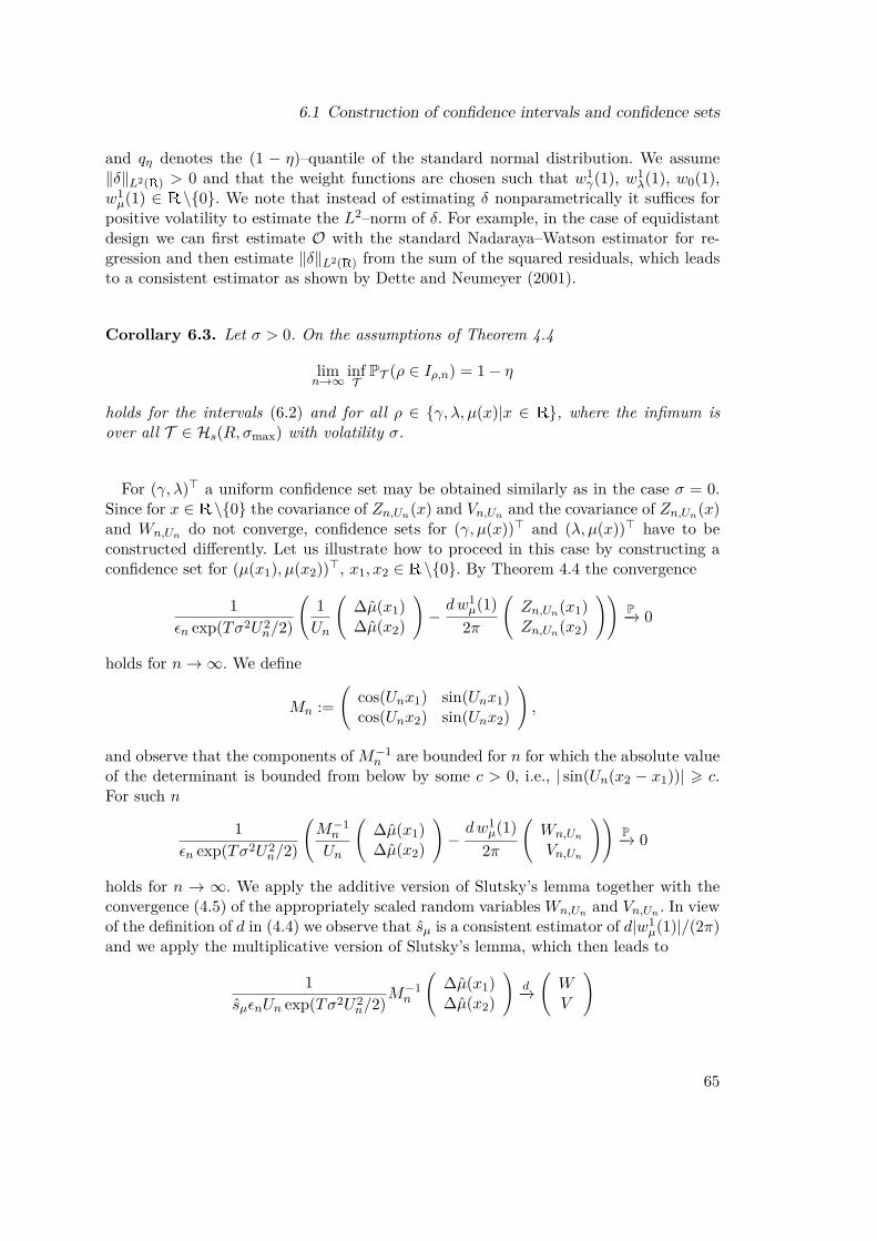
6.1 Construction of confidence intervals and confidence sets
and qη denotes the (1 − η)–quantile of the standard normal distribution. We assume‖δ‖L2(R) > 0 and that the weight functions are chosen such that w1
γ(1), w1λ(1), w0(1),
w1µ(1) ∈ R \0. We note that instead of estimating δ nonparametrically it suffices for
positive volatility to estimate the L2–norm of δ. For example, in the case of equidistantdesign we can first estimate O with the standard Nadaraya–Watson estimator for re-gression and then estimate ‖δ‖L2(R) from the sum of the squared residuals, which leadsto a consistent estimator as shown by Dette and Neumeyer (2001).
Corollary 6.3. Let σ > 0. On the assumptions of Theorem 4.4
limn→∞
infT
PT (ρ ∈ Iρ,n) = 1− η
holds for the intervals (6.2) and for all ρ ∈ γ, λ, µ(x)|x ∈ R, where the infimum isover all T ∈ Hs(R, σmax) with volatility σ.
For (γ, λ)> a uniform confidence set may be obtained similarly as in the case σ = 0.Since for x ∈ R \0 the covariance of Zn,Un(x) and Vn,Un and the covariance of Zn,Un(x)and Wn,Un do not converge, confidence sets for (γ, µ(x))> and (λ, µ(x))> have to beconstructed differently. Let us illustrate how to proceed in this case by constructing aconfidence set for (µ(x1), µ(x2))>, x1, x2 ∈ R \0. By Theorem 4.4 the convergence
1εn exp(Tσ2U2
n/2)
(1Un
(∆µ(x1)∆µ(x2)
)−dw1
µ(1)2π
(Zn,Un(x1)Zn,Un(x2)
))P−→ 0
holds for n→∞. We define
Mn :=(
cos(Unx1) sin(Unx1)cos(Unx2) sin(Unx2)
),
and observe that the components ofM−1n are bounded for n for which the absolute value
of the determinant is bounded from below by some c > 0, i.e., | sin(Un(x2 − x1))| > c.For such n
1εn exp(Tσ2U2
n/2)
(M−1n
Un
(∆µ(x1)∆µ(x2)
)−dw1
µ(1)2π
(Wn,Un
Vn,Un
))P−→ 0
holds for n → ∞. We apply the additive version of Slutsky’s lemma together with theconvergence (4.5) of the appropriately scaled random variablesWn,Un and Vn,Un . In viewof the definition of d in (4.4) we observe that sµ is a consistent estimator of d|w1
µ(1)|/(2π)and we apply the multiplicative version of Slutsky’s lemma, which then leads to
1sµεnUn exp(Tσ2U2
n/2)M−1n
(∆µ(x1)∆µ(x2)
)d−→(WV
)
65
6 Applications
for n→∞ such that | sin(Un(x2 − x1))| > c. We define
Bn := (µ(x1), µ(x2))> +MnsµεnUn exp(Tσ2U2n/2)(x, y)>|x2 + y2 6 kη,
where kη denotes the (1−η)–quantile of the chi–squared distribution χ22 with two degrees
of freedom. Then
lim| sin(Un(x2−x1))|>c
n→∞
PT ((µ(x1), µ(x2))> ∈ Bn) = 1− η
holds for all T ∈ Gs(R, σmax) ∩ σ > 0.
6.2 Inference on the volatility
In this section, we test the hypothesesH0 : T ∈ σ = σ0∩Hs(R, σmax) against the alter-nativeH1 : T ∈ |σ−σ0| > τ∩Hs(R, σmax) for σ0 ∈ [0, σmax] and τ > 0. For η ∈ (0, 1/2],the test reaches asymptotically the level η, i.e., limn→∞ supT ∈H0 ET [ϕσ0 ] = η. Moreover,the error of the second kind vanishes asymptotically, i.e., limn→∞ supT ∈H1 ET [1−ϕσ0 ] =0. This family of tests can be used to construct a confidence set for σ.For σ0 > 0 the most natural test statistic is the following. In order to apply the
uniform version of Theorem 4.4 under H0 we choose a sequence of cut–off values Un suchthat εnU2
n exp(Tσ20U
2n/2)→ 0 and εnU s+1
n exp(Tσ20U
2n/2)→∞ as n→∞. Let σ2 be the
estimator corresponding to this cut–off value Un. Since we assume that T ∈ Hs(R, σmax),we have σ ∈ [0, σmax]. We ensure σ2 ∈ [0, σ2
max] by taking the maximum with zero andthe minimum with σ2
max. Likewise we ensure γ ∈ [−R,R] and λ ∈ [0, R]. We assume‖δ‖L2(R) > 0, choose a weight function with w1
σ(1) 6= 0 and define
Sσ0 := U2n(σ2 − σ2
0)dσ0 εn exp(Tσ2
0U2n/2)
, dσ0 :=√
2 |w1σ(1)| ‖δ‖L2(R)
exp(T (σ20/2 + γ − λ))T 2σ2
0.
Under H0 the test statistic Sσ0 converges uniformly in distribution to a standard normalrandom variable by the uniform version of Theorem 4.4. We decompose
Sσ0 = U2n∆σ2
dσ0 εn exp(Tσ20U
2n/2)
+ U2n(σ2 − σ2
0)dσ0 εn exp(Tσ2
0U2n/2)
. (6.3)
We will show that for σ 6 σ0−τ the first term converges uniformly in probability to zero.The approximation error contributes a term that converges deterministically to zero bythe bound (4.29) and by the assumption εnU
s+1n exp(Tσ2
0U2n/2) → ∞ as n → ∞. The
remainder term of the stochastic error in the first summand of (6.3) converges uniformlyin probability to zero by Section 5.4 and the linearized stochastic error by the followinglemma.
Lemma 6.4. Let δ ∈ L∞(R). Let wU ∈ L∞([0, 1],C) be Riemann–integrable and let
66
6.2 Inference on the volatility
there be a constant C > 0 such that ‖wU‖∞ 6 C for all U > 1. Then for all κ, τ > 0
supT ∈Hs(R,σ0−τ)
PT(∣∣∣∣ 1εn exp(Tσ2
0U2/2)
∫ 1
0wU (u)Ln,U (u)du
∣∣∣∣ > κ
)→ 0,
as U →∞
Proof. It is equivalent to consider for all τ ′ > 0 the supremum over Hs(R,√σ2
0 − τ ′),such that σ2 6 σ2
0 − τ ′ is satisfied for each T . By (4.16) we have
supT
1ε2n exp(Tσ2
0U2)E[∫ 1
0wU (u)Ln,U (u)du
∫ 1
0wU (v)Ln,U (v)dv
]
= supT
2πU4 exp(2T (λ− γ − σ2/2))T 2 exp(Tσ2
0U2)
∫ 1
0
∫ 1
0fU (u)fU (v)
F−1(δ(y + θ)2)(U(u− v))eTσ2U2(u2+v2)/2dudv
64πU4 exp(6TR)C2
T 2 exp(Tτ ′U2) ‖F−1δ2‖∞ → 0,
as U →∞, where we used ‖fU‖∞ 6√
2C exp(TR).
We have seen that for σ 6 σ0 − τ the first term in (6.3) converges to zero uni-formly in probability. The second term is d−1
σ0 times a deterministic sequence convergingto −∞. We note that dσ0 is bounded from above and below. Consequently, it holdslimn→∞ infHs(R,σ0−τ) P(Sσ0 < c) = 1 for all c ∈ R. We would like to make a similarstatement in the case σ > σ0 + τ . Unfortunately for σ > σ0 the variance of Ln,Un(1)does not converge to zero. So it is not possible to find a bound like in Proposition 3.3,which converges to zero. Consequently, the remainder term cannot be controlled byLemma 4.10. We modify the test statistic in the following way. We choose σ > σmax andlet Un be a cut–off value with εnU2
n exp(T σ2U2n/2)→ 0 and εnU s+1
n exp(T σ2U2n/2)→∞
as n→∞. We further assume that
U2n exp(−T σ2U2
n/2)U2n exp(−Tσ2
0U2n/2)
→∞. (6.4)
This can for example be ensured by choosing the cut–off values Un and Un accordingto (4.6) with α and α > α, respectively. Let σ2 be the estimator of σ2 corresponding tothe cut–off value Un. We define
Sσ0 := Sσ0 + U2n(σ2 − σ2
0)εn exp(T σ2U2
n/2)(6.5)
= Sσ0 + U2n(σ2 − σ2)
εn exp(T σ2U2n/2)
+ U2n(σ2 − σ2
0)εn exp(T σ2U2
n/2). (6.6)
Under H0 the statistic Sσ0 can be written as in Lemma 5.4. The second term in (6.5)
67
6 Applications
converges uniformly in probability to zero. Thus, under H0 the modified statistic Sσ0
converges uniformly in distribution to a standard normal random variable by Lemma 5.4.For σ 6 σ0 − τ the second term in (6.6) converges uniformly in probability to zeroand the third term is deterministic sequence converging to −∞. As for Sσ0 it holdslimn→∞ infHs(R,σ0−τ) P(Sσ0 < c) = 1 for all c ∈ R. But now we are also able to make asimilar statement for σ > σ0 + τ . Since we bounded the estimators Sσ0 cannot divergefaster than ε−1
n U2n exp(−Tσ2
0U2n/2). For σ ∈ [0, σmax] the second term in (6.6) converges
uniformly in probability to zero. Owing to (6.4) the third term in (6.6) tends to infinityfaster than the bound of Sσ0 . It holds limn→∞ infT P(Sσ0 > c) = 1 for all c ∈ R, wherethe infimum is over all T ∈ Hs(R, σmax) with σ > σ0 + τ .Let qη denote the (1 − η)–quantile of the standard normal distribution. For σ0 ∈
(0, σmax) we define the tests
ϕσ0 :=
0, if |Sσ0 | 6 qη/21, if |Sσ0 | > qη/2
, ϕσmax :=
0, if Sσmax > q1−η1, if Sσmax < q1−η
.
For σ0 = 0 we would like to apply Theorem 4.1. To this end, we choose the cut–offvalue Un such that εnU5/2
n → 0 and εnU(2s+5)/2n → ∞. Let σ2 be the estimator corre-
sponding to this cut–off value Un, where σ2 ∈ [0, σ2max] is ensured. We assume that δ is
positive on [−TR, TR] and define
S0 := U1/2n σ2
d0 εn+ U2
nσ2
εn exp(Tσ2maxU
2n/2)
,
d0 := 2√πδ(T γ)
exp(T (γ − λ))T
(∫ 1
0u4w1
σ(u)2du)1/2
.
Under H0 : σ2 = 0 the test statistic S0 converges uniformly in distribution to a standardnormal random variable by a similar argument as for Sσ0 . We observe that the first termof S0 is nonnegative. Under H1 : σ > τ the second term of S0 may be decomposed asin (6.6) into a part that converges uniformly in distribution to zero and into a determin-istic sequence converging to infinity. It holds limn→∞ infT P(S0 > c) = 1 for all c ∈ R,where the infimum is over all T ∈ Hs(R, σmax) with σ > τ . We define the test
ϕ0 :=
0, if S0 6 qη1, if S0 > qη
.
Since we have a test on σ = σ0 for each σ0 ∈ [0, σmax], we may use this familyof tests to define a confidence set for σ. We define Mn := σ|ϕσ = 0 and obtainlimn→∞ infT PT (σ ∈ Mn) = 1− η, where the infimum is over all T ∈ Hs(R, σmax) withvolatility σ. The set Mn is not necessarily an interval. For σ0 ∈ (0, σmax) the cut–offvalue Un may be chosen as a continuous function of σ0 by (4.6). The estimators σ2, γand λ depend continuously on the cut–off value Un, which can be seen by substitutingv = u/U in (2.12), (2.13) and (2.14) and applying the continuity theorem on parameter
68

6.2 Inference on the volatility
dependent integrals. Thus, S : (0, σmax)→ R, σ 7→ Sσ is continuous and Mn ∩ (0, σmax)may be written as the preimage S−1([−qη/2, qη/2]) of the continuous function S.
69

7 Simulations and empirical resultsIn the last chapter, we derived asymptotic confidence intervals for the volatility, thedrift, the intensity and pointwise for the jump density. This chapter is concerned withthe application of the results in simulations and to option data of the German DAX index.It is based on the results that will appear in Söhl and Trabs (2012b), where in additionto finite intensity Lévy processes also self–decomposable Lévy processes are treated.More precisely, the paper is complemented by confidence intervals for the method byTrabs (2012) and their application in simulations and to option data. We slightly adjustthe theoretical concepts of the last chapter and thus enhance the performance of themethod in practice. The main difference concerns the construction of the confidence sets.Applying the confidence intervals in simulations with sample sizes as in available datashows that they are to conservative. In the proof of the asymptotic normality, we haveseen that the asymptotic variances are completely determined by the linearized stochasticerrors and that the remainder terms and the approximation errors are asymptoticallynegligible. Replacing the asymptotic variances of the linearized stochastic errors by thefinite sample variances certainly gives a more precise measure of how the estimatorsdeviate from the true value. So we base our confidence intervals on the finite samplevariances of the linearized stochastic errors. However, this still leads to asymptotic andnot to finite sample confidence intervals since we continue to take advantage of theremainder terms and the approximation errors being asymptotically negligible. The soconstructed intervals perform well in terms of size and coverage probabilities as we willdemonstrate by simulations from the model by Merton (1976).Our estimators for (σ2, γ, ν) are constructed essentially as described in Section 2.2,
but some modifications are introduced which improve their numerical performance. Asshown in simulations these improvements reduce the mean squared error of the estima-tors significantly. In contrast to the method by Cont and Tankov (2004b) the spectralcalibration method is a straightforward algorithm, where no minimization problem hasto be solved. Therefore, the method is quite fast owing to the Fast Fourier transform(FFT). In this chapter, we concentrate on the application of the method to realisticsample sizes. In a related framework of a jump–diffusion Libor model, Belomestny andSchoenmakers (2011) study the application of the spectral calibration method to finitesample data sets.We use data of vanilla options on the German DAX index. Considering options
with different maturities, the model achieves good calibration results in the sense thatthe residuals between the given data and the calibrated model are small. Since theBlumenthal–Getoor index equals zero in our model, the calibration based on option databehaves quite differently from the case of high–frequency observations under the histor-ical measure, where Aït-Sahalia and Jacod (2009) find evidence that the Blumenthal–
71
7 Simulations and empirical results
Getoor index is larger than one. Applying the calibration to a sequence of trading days,we obtain the evolution of the model parameters in time. The estimators seem to bestable with respect to the spot time.This chapter is organized as follows: In Section 7.1 we specify the estimation method
used in the simulations and for the option data of the German DAX index. In Section 7.3the confidence intervals are derived and their performance is assessed in simulations. Weapply the method to the data and discuss our results in Section 7.4. The more technicalpart of determining the finite sample variances is deferred to Section 7.5.
7.1 The estimation method in applicationsA typical parametric submodel is given by Example 7.1. We will use it to study theperformance of estimation method in simulations.
Example 7.1 (Merton model). Merton (1976) introduced the first exponential Lévymodel. Therein, the jumps are normally distributed with intensity λ > 0:
ν(x) = λ√2πv
exp(−(x− η)2
2v2
), x ∈ R.
A realistic choice of the parameters is η = −0.1, v = 0.2 and λ = 5. Together withthe volatility σ = 0.1 this determines the drift to be γ = 0.379 using the martingalecondition (2.8).
We will use the estimators σ2, γ and λ as defined in (2.12)–(2.14). In this chapter,we will use the estimator ν obtained by plugging in σ2, γ and λ in the estimationformula (2.23) for ν of the slightly modified estimation method. This has the advantagethat ν can be estimated directly without estimating first µ by (2.16) and then multiplyingby e−x. This direct estimation turns out to be more stable in simulations with smallsample sizes.Note that correction steps are necessary to satisfy non–negativity of the jump density
and the martingale condition (2.8). If the latter one would be violated, the right–handside of the pricing formula (2.9) could have a singularity at zero and thus we could notapply the inverse Fourier transform to obtain an option function O from the calibration.A critical question is the choice of the regularization parameter U . As a benchmark, we
use in simulations an oracle cut–off value, that is U minimizes the discrepancy betweenthe estimators and the true values of σ2, γ and ν measured in an L2–loss. To calibratereal data, we employ the simple least squares approach
U∗ := arginfU RSS(U) with the residual sum of squares
RSS(U) :=n∑j=1|OU (xj)−Oj |2, (7.1)
where OU is the option function corresponding to the characteristic triplet estimated by
72
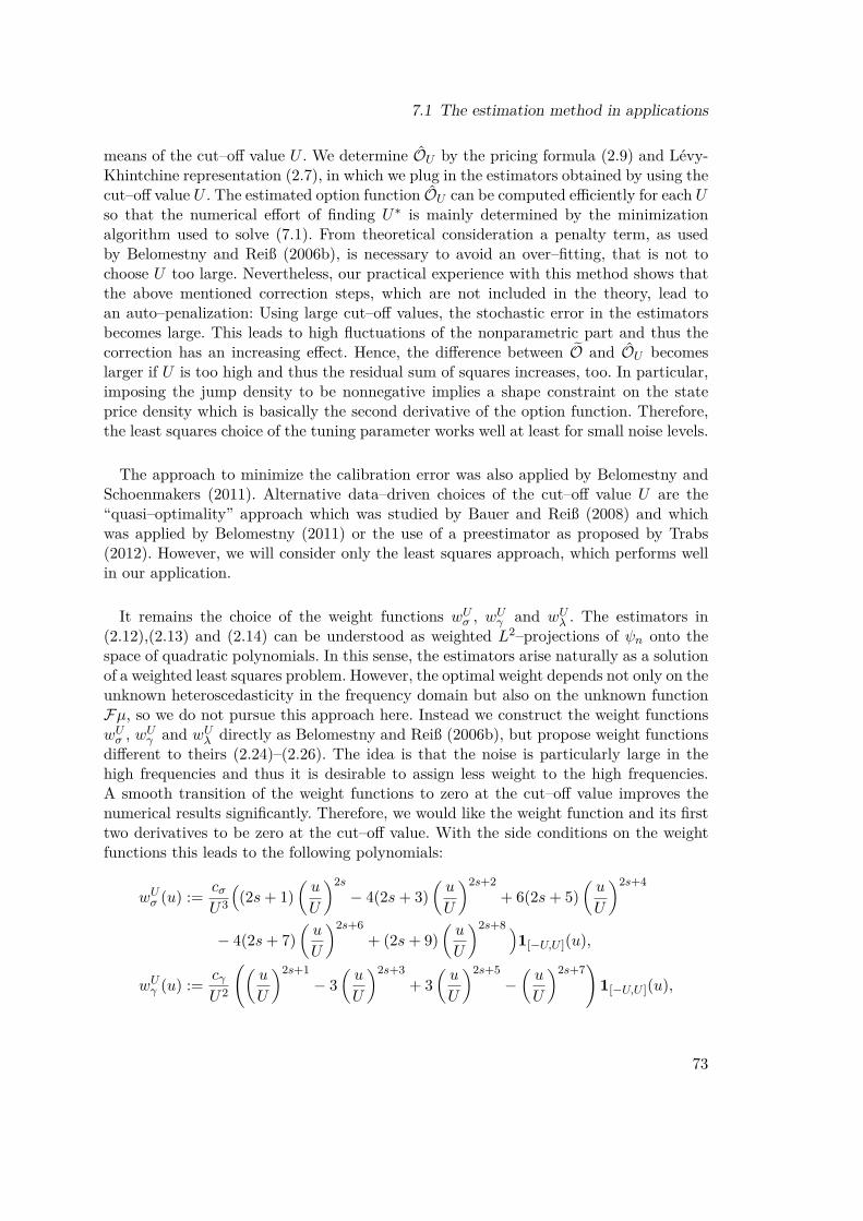
7.1 The estimation method in applications
means of the cut–off value U . We determine OU by the pricing formula (2.9) and Lévy-Khintchine representation (2.7), in which we plug in the estimators obtained by using thecut–off value U . The estimated option function OU can be computed efficiently for each Uso that the numerical effort of finding U∗ is mainly determined by the minimizationalgorithm used to solve (7.1). From theoretical consideration a penalty term, as usedby Belomestny and Reiß (2006b), is necessary to avoid an over–fitting, that is not tochoose U too large. Nevertheless, our practical experience with this method shows thatthe above mentioned correction steps, which are not included in the theory, lead toan auto–penalization: Using large cut–off values, the stochastic error in the estimatorsbecomes large. This leads to high fluctuations of the nonparametric part and thus thecorrection has an increasing effect. Hence, the difference between O and OU becomeslarger if U is too high and thus the residual sum of squares increases, too. In particular,imposing the jump density to be nonnegative implies a shape constraint on the stateprice density which is basically the second derivative of the option function. Therefore,the least squares choice of the tuning parameter works well at least for small noise levels.
The approach to minimize the calibration error was also applied by Belomestny andSchoenmakers (2011). Alternative data–driven choices of the cut–off value U are the“quasi–optimality” approach which was studied by Bauer and Reiß (2008) and whichwas applied by Belomestny (2011) or the use of a preestimator as proposed by Trabs(2012). However, we will consider only the least squares approach, which performs wellin our application.
It remains the choice of the weight functions wUσ , wUγ and wUλ . The estimators in(2.12),(2.13) and (2.14) can be understood as weighted L2–projections of ψn onto thespace of quadratic polynomials. In this sense, the estimators arise naturally as a solutionof a weighted least squares problem. However, the optimal weight depends not only on theunknown heteroscedasticity in the frequency domain but also on the unknown functionFµ, so we do not pursue this approach here. Instead we construct the weight functionswUσ , wUγ and wUλ directly as Belomestny and Reiß (2006b), but propose weight functionsdifferent to theirs (2.24)–(2.26). The idea is that the noise is particularly large in thehigh frequencies and thus it is desirable to assign less weight to the high frequencies.A smooth transition of the weight functions to zero at the cut–off value improves thenumerical results significantly. Therefore, we would like the weight function and its firsttwo derivatives to be zero at the cut–off value. With the side conditions on the weightfunctions this leads to the following polynomials:
wUσ (u) := cσU3
((2s+ 1)
(u
U
)2s− 4(2s+ 3)
(u
U
)2s+2+ 6(2s+ 5)
(u
U
)2s+4
− 4(2s+ 7)(u
U
)2s+6+ (2s+ 9)
(u
U
)2s+8 )1[−U,U ](u),
wUγ (u) := cγU2
((u
U
)2s+1− 3
(u
U
)2s+3+ 3
(u
U
)2s+5−(u
U
)2s+7)
1[−U,U ](u),
73
7 Simulations and empirical results
wUλ (u) := cλU
((2s+ 3)
(u
U
)2s− 4(2s+ 5)
(u
U
)2s+2+ 6(2s+ 7)
(u
U
)2s+4
− 4(2s+ 9)(u
U
)2s+6+ (2s+ 11)
(u
U
)2s+8 )1[−U,U ](u).
The constants cσ, cγ , cλ ∈ R are determined by the normalization conditions∫ U
−U
−u2
2 wUσ (u) du = 1,∫ U
−UuwUγ (u) du = 1 and
∫ U
−UwUλ (u) du = 1.
The parameter s reflects the a priori knowledge about the smoothness of ν and can bechosen equal to two. The gain of the new weight functions is discussed in Section 7.2.To estimate directly the jump density ν and not only the exponential scaled version µ,
we use ψ(u+ i) instead of ψ(u) as discussed above. Therefore, we define the estimator
ν(x) := F−1[(ψn(u+ i) + σ2
2 u2 − iγu+ λ
)wUν (u)
](x), (7.2)
where ψn(u + i) is the empirical version of ψ(u + i) and wUν is a flat top kernel withsupport [−U,U ]:
wUν (u) := F
(u
U
)with F (u) :=
1, |u| ≤ 0.05,exp
(− exp(−(|u|−0.05)−2)
(|u|−1)2
), 0.05 < |u| < 1,
0, |u| ≥ 1.(7.3)
To evaluate the integrals in (2.12) to (2.14), it suffices to apply the trapezoidal rule.The inverse Fourier transformation in (7.2) can be efficiently computed using the FFT–algorithm. Therefore, depending on the interpolation method which is applied to ob-tain On, the whole estimation procedure is very fast. Finally, we note that the cut–offvalue can be chosen differently for each quantity σ2, γ, λ and ν.
7.2 Simulations
Let us first describe the setting of all of our simulations. In view of the higher concen-tration of European options at the money, the design points x1, . . . , xn are chosento be the k/(n + 1)–quantiles, k = 1, . . . , n, of a normal distribution with mean zeroand variance 1/2. The observations Oj are computed from the characteristic functionϕT using the fast Fourier transform. The additive noise consists of independent, normaland centered random variables with variance δ2
j = |τO(xj)|2 for some relative noise levelτ > 0. We use the notation ‖δ‖l∞ := supj δj . By choosing the sample size n and thedeviation parameter τ , we determine the noise level of the observations. According to theexisting theoretical results by Belomestny and Reiß (2006a) as well as by Trabs (2012),
74
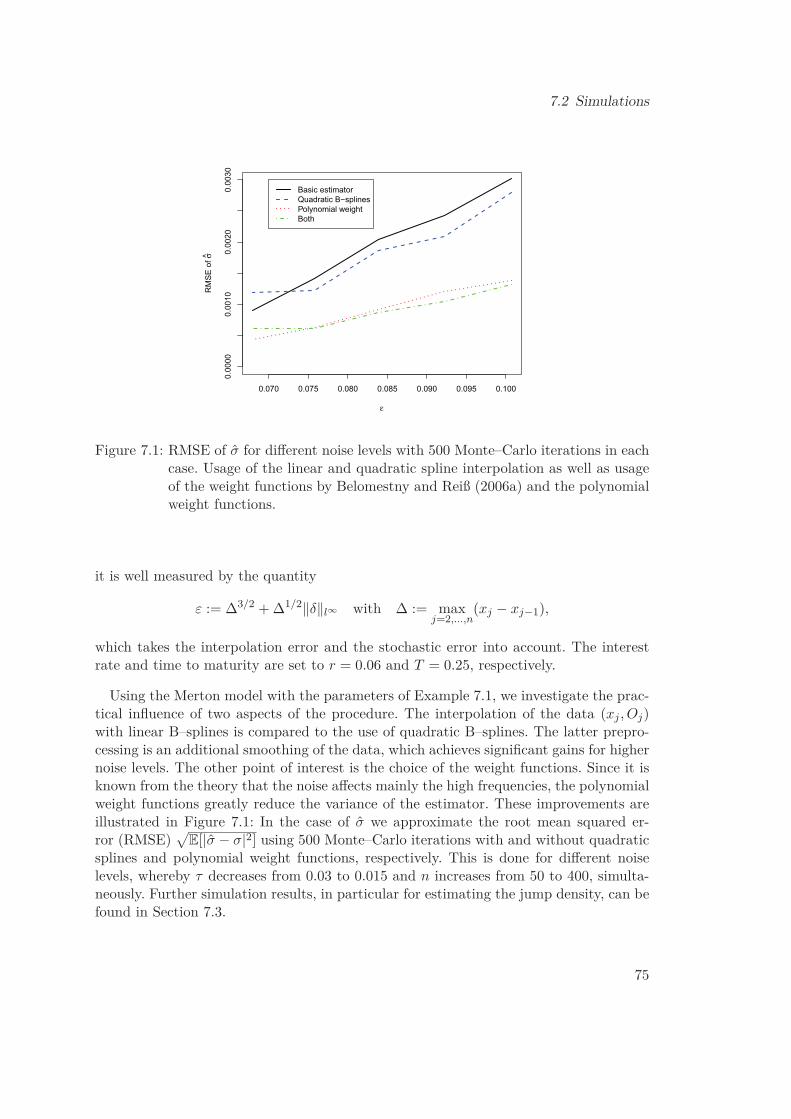
7.2 Simulations
ε
σ
Figure 7.1: RMSE of σ for different noise levels with 500 Monte–Carlo iterations in eachcase. Usage of the linear and quadratic spline interpolation as well as usageof the weight functions by Belomestny and Reiß (2006a) and the polynomialweight functions.
it is well measured by the quantity
ε := Δ3/2 +Δ1/2‖δ‖l∞ with Δ := maxj=2,...,n
(xj − xj−1),
which takes the interpolation error and the stochastic error into account. The interestrate and time to maturity are set to r = 0.06 and T = 0.25, respectively.
Using the Merton model with the parameters of Example 7.1, we investigate the prac-tical influence of two aspects of the procedure. The interpolation of the data (xj , Oj)with linear B–splines is compared to the use of quadratic B–splines. The latter prepro-cessing is an additional smoothing of the data, which achieves significant gains for highernoise levels. The other point of interest is the choice of the weight functions. Since it isknown from the theory that the noise affects mainly the high frequencies, the polynomialweight functions greatly reduce the variance of the estimator. These improvements areillustrated in Figure 7.1: In the case of σ we approximate the root mean squared er-ror (RMSE)
√E[|σ − σ|2] using 500 Monte–Carlo iterations with and without quadratic
splines and polynomial weight functions, respectively. This is done for different noiselevels, whereby τ decreases from 0.03 to 0.015 and n increases from 50 to 400, simulta-neously. Further simulation results, in particular for estimating the jump density, can befound in Section 7.3.
75
7 Simulations and empirical results
7.3 Confidence intervals
While we have constructed confidence intervals based on the asymptotic variance inSection 6.1, we want to construct in this section confidence intervals based on the finitesample variance of the linearized stochastic errors. The construction is in the spirit ofthe asymptotic analysis of Chapter 4 in the sense that the remainder terms and theapproximation errors are not taken into account. But given this, it is an independent,rather direct approach to the construction of confidence sets, which transfers easily tosimilar methods. Presented in a less rigorous manner, it is a practical method to obtainconfidence sets.
Let us consider σ2 first. All other parameters can be treated similarly. By the under-smoothing approach to the construction of confidence intervals, we neglect the approxi-mation error and consider the stochastic error only, compare (2.29),
σ2 − σ2 ≈∫ U
−URe(∆ψn(u))wUσ (u) du (7.4)
with ∆ψn := ψn − ψ. The term ∆ψn is a logarithm, which we approximate by
∆ψn(u) = 1T
log(1 + iu(1 + iu)F On(u)
1 + iu(1 + iu)F O(u)
)≈ iu(1 + iu)TϕT (u− i)(F On −F O)(u) (7.5)
using log(1 + x) ≈ x for small x. Apply the approximation (7.5) to the right–hand sideof (7.4) yields the linearized stochastic error.
To analyze the deviation F On−F O in the linearized stochastic error, we assume thatthe noise levels of the observations (2.6) are given by the values δj = δ(xj), j = 1, . . . , n,of some function δ : R → R+. The observation points are assumed to be the quantilesxj = H−1(j/(n + 1)), j = 1, . . . , n, of a distribution with c.d.f. H : R → [0, 1] andp.d.f. h. For the definition of the confidence intervals we need the generalized noise level
%(x) = δ(x)/√h(x), (7.6)
which incorporates the noise of the observations as well as their distribution. Insteadof assuming that the observation points are given by the quantiles of h one may alsoassume that the observation points are sampled randomly from the density h. On theseconditions Brown and Low (1996) showed the asymptotic equivalence in the sense ofLe Cam of the nonparametric regression model (2.6) and the white noise model dZn(x) =O(x) dx + n−1/2%(x) dW (x) with a two–sided Brownian motion W . This asymptoticequivalence has been discussed where the Gaussian white noise model (2.30) is introducedin Chapter 2. Zn is an empirical version of the antiderivative of O. In that sense we define
F On(u) := F [ dZn](u) = F O(u) + n−1/2∫R
eiux%(x) dW (x).
76
7.3 Confidence intervals
Combining (7.5) with this asymptotic equivalence, we can approximate
∆ψn(u) ≈ 1√n
iu(1 + iu)TϕT (u− i)
∫R
eiux%(x) dW (x) =: 1√nL(u).
Defining fσ,U (u) := wUσ (u)iu(1 + iu)/(TϕT (u− i)), we obtain with the above considera-tions and by changing the order of integration
σ2 − σ2 ≈ 1√n
∫ U
−URe(L(u))wUσ (u) du = 2π√
n
∫R
Re(F−1 fσ,U (−x)
)%(x) dW (x).
For σ2 we calculate the finite sample variance s2σ2 of the linearized stochastic errors using
the Itô isometry
s2σ2 = 1
nE
(∫ U
−URe(L(u))wUσ (u) du
)2
= 4π2
nE[(∫
R
Re(F−1 fσ,U (−x)
)%(x) dW (x)
)2]
= 4π2
n
∫R
(Re(F−1 fσ,U (−x)
)%(x)
)2dx. (7.7)
Similar results for γ, λ and ν(x0), x0 ∈ R, are derived in Section 7.5. The correspondingfinite sample variances s2
γ , s2λ and s2
ν(x0) are given by (7.9), (7.10) and (7.11), respectively.In contrast to the asymptotic normality results in Chapter 4, we do not have to distin-guish between the cases x0 = 0 and x0 6= 0 in the finite sample analysis. An advantageof this way of deriving the variance and thus of constructing confidence sets is that itcan easily be transferred to similar methods. For the calibration of self–decomposableLévy processes this is done in Söhl and Trabs (2012b).To construct confidence intervals for ϑ ∈ σ2, γ, λ, ν(x0), we need an estimate sϑ of
the standard deviation. To this end, the function fq,U has to be replaced by its empiricalversion. Since the only unknown quantity involved is ϕT , it suffices to plug in an estimatorfor the characteristic function. Either one uses the Lévy-Khintchine representation (2.7)replacing the true characteristic triplet by their estimators or ϕT is estimated by theempirical version ψn in (2.11) and (2.19), respectively. We will follow the second approachsince the estimate is independent of the cut–off value U and thus may lead to more stableresults. To compute the noise function %, the density h of the distribution of the strikesis necessary while in practice there is only a discrete set of strike prices. The density hcan be estimated from the observation points (xj)j=1,...,n using some standard densityestimation method. We will apply a triangular kernel estimator, where the bandwidth ischosen by Silverman’s rule of thumb. The (1− η)–confidence intervals for a level η > 0are then given by
Iϑ := [ϑ− sϑqη/2, ϑ+ sϑqη/2], (7.8)
where qη denotes the (1 − η)–quantile of the standard normal distribution. Naturally,
77
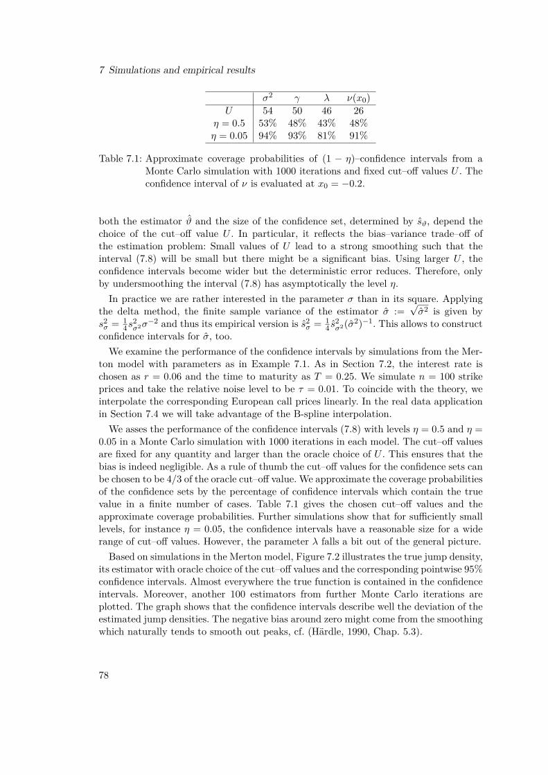
7 Simulations and empirical results
σ2 γ λ ν(x0)U 54 50 46 26
η = 0.5 53% 48% 43% 48%η = 0.05 94% 93% 81% 91%
Table 7.1: Approximate coverage probabilities of (1 − η)–confidence intervals from aMonte Carlo simulation with 1000 iterations and fixed cut–off values U . Theconfidence interval of ν is evaluated at x0 = −0.2.
both the estimator ϑ and the size of the confidence set, determined by sϑ, depend thechoice of the cut–off value U . In particular, it reflects the bias–variance trade–off ofthe estimation problem: Small values of U lead to a strong smoothing such that theinterval (7.8) will be small but there might be a significant bias. Using larger U , theconfidence intervals become wider but the deterministic error reduces. Therefore, onlyby undersmoothing the interval (7.8) has asymptotically the level η.In practice we are rather interested in the parameter σ than in its square. Applying
the delta method, the finite sample variance of the estimator σ :=√σ2 is given by
s2σ = 1
4s2σ2σ−2 and thus its empirical version is s2
σ = 14 s
2σ2(σ2)−1. This allows to construct
confidence intervals for σ, too.We examine the performance of the confidence intervals by simulations from the Mer-
ton model with parameters as in Example 7.1. As in Section 7.2, the interest rate ischosen as r = 0.06 and the time to maturity as T = 0.25. We simulate n = 100 strikeprices and take the relative noise level to be τ = 0.01. To coincide with the theory, weinterpolate the corresponding European call prices linearly. In the real data applicationin Section 7.4 we will take advantage of the B-spline interpolation.We asses the performance of the confidence intervals (7.8) with levels η = 0.5 and η =
0.05 in a Monte Carlo simulation with 1000 iterations in each model. The cut–off valuesare fixed for any quantity and larger than the oracle choice of U . This ensures that thebias is indeed negligible. As a rule of thumb the cut–off values for the confidence sets canbe chosen to be 4/3 of the oracle cut–off value. We approximate the coverage probabilitiesof the confidence sets by the percentage of confidence intervals which contain the truevalue in a finite number of cases. Table 7.1 gives the chosen cut–off values and theapproximate coverage probabilities. Further simulations show that for sufficiently smalllevels, for instance η = 0.05, the confidence intervals have a reasonable size for a widerange of cut–off values. However, the parameter λ falls a bit out of the general picture.Based on simulations in the Merton model, Figure 7.2 illustrates the true jump density,
its estimator with oracle choice of the cut–off values and the corresponding pointwise 95%confidence intervals. Almost everywhere the true function is contained in the confidenceintervals. Moreover, another 100 estimators from further Monte Carlo iterations areplotted. The graph shows that the confidence intervals describe well the deviation of theestimated jump densities. The negative bias around zero might come from the smoothingwhich naturally tends to smooth out peaks, cf. (Härdle, 1990, Chap. 5.3).
78
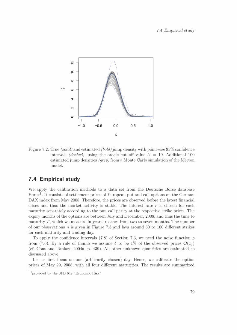
7.4 Empirical study
ν
Figure 7.2: True (solid) and estimated (bold) jump density with pointwise 95% confidenceintervals (dashed), using the oracle cut–off value U = 19. Additional 100estimated jump densities (grey) from a Monte Carlo simulation of the Mertonmodel.
7.4 Empirical studyWe apply the calibration methods to a data set from the Deutsche Börse databaseEurex1. It consists of settlement prices of European put and call options on the GermanDAX index from May 2008. Therefore, the prices are observed before the latest financialcrises and thus the market activity is stable. The interest rate r is chosen for eachmaturity separately according to the put–call parity at the respective strike prices. Theexpiry months of the options are between July and December, 2008, and thus the time tomaturity T , which we measure in years, reaches from two to seven months. The numberof our observations n is given in Figure 7.3 and lays around 50 to 100 different strikesfor each maturity and trading day.To apply the confidence intervals (7.8) of Section 7.3, we need the noise function
from (7.6). By a rule of thumb we assume δ to be 1% of the observed prices O(xj)(cf. Cont and Tankov, 2004a, p. 439). All other unknown quantities are estimated asdiscussed above.Let us first focus on one (arbitrarily chosen) day. Hence, we calibrate the option
prices of May 29, 2008, with all four different maturities. The results are summarized1provided by the SFB 649 “Economic Risk”
79

7 Simulations and empirical results
Figure 7.3: Number of observed prices of put and call options during May, 2008.
in Table 7.2 and Figure 7.4. Using the complete estimation of the model, we generatethe corresponding option functions O. They are graphically compared to the given datapoints and we calculate the residual sum of squares RSS = RSS(U∗) as defined in (7.1).For all maturities the method yields good fits to the data.In all maturities the jump density has more weight on the negative half line and thus
there are more negative than positive jumps priced into the options. This coincides withthe empirical findings in the literature (see eg, Cont and Tankov, 2004a). Due to thepositivity correction, the jump densities might look unsmooth, where they are close tozero. This problem might be circumvented by adding smoothness constraints. However,the construction of confidence intervals would then be much more difficult. Hence, thistopic is left open for further research.In view of the parametric calibration of their CGMY model, Carr et al. (2002) sug-
gested that risk–neutral processes of assets should be modeled by pure jump processeswith finite variation. Now, the nonparametric approach shows that the model is able toreproduce the option data. Note that the Blumenthal–Getoor index equals zero, whichis in contrast to the investigation of high-frequency historical data, where Aït-Sahaliaand Jacod (2009) estimated a jump activity index larger than one.Next we investigate the calibration across different trading days. By considering more
than one day we investigate the stability of the estimation procedure. Moreover, calibrat-ing the model across the trading days in May, 2008, shows the development of the modelalong the time line and with small changes in the maturities. To profit from the higherobservation numbers, we apply the calibration procedure to the options with maturityin September and December.The estimations of the parameters are displayed in Figure 7.5. Note that we do not
smooth over time. Furthermore, the 95% confidence intervals for the December optionsare shown. The estimated volatility σ fluctuates around 0.1 and 0.12. The confidencesets imply that there is no significant difference between the two maturities. Both γ andλ decrease for higher durations: On the one hand the curves of December lie significantly
80
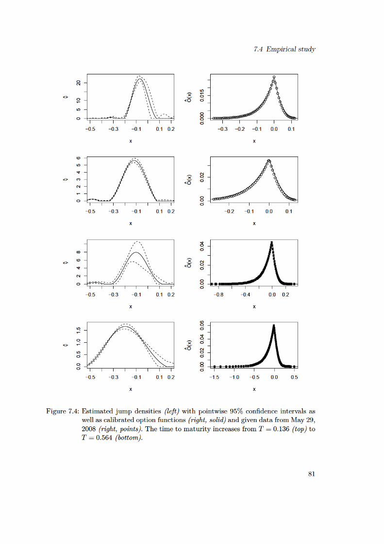
−0.5 −0.3 −0.1 0.1 0.2
0 5 10
20
x
ν
−0.3 −0.2 −0.1 0.0 0.1
0.000
0.015
x
O^(x)
−0.5 −0.3 −0.1 0.1 0.2
0 1 2 3 4 5 6
x
ν
−0.2 −0.1 0.0 0.1
0.00
0.02
x
O^(x)
7.4Empiricalstudy
−0.5 −0.3 −0.1 0.1 0.2
0 2 4 6 8
x
ν
ll
llllllllllllllllllllllllllllllllllllll
llllllllllllllllllllllllllllllllllllll
lllllllllllllllllllllll
−0.8 −0.4 0.0 0.2
0.00
0.02
0.04
x
O^(x)
−0.5 −0.3 −0.1 0.1 0.2
0.0 0.5 1.0 1.5
x
ν
llllllllllllllllllllll
lllllllllll
lllllllllllll
lllllllllllllllllllllllllllllllllllllllllllllllllllllll
lllll
−1.5 −1.0 −0.5 0.0 0.5
0.00 0.02 0.04 0.06
x
O^(x)
Figure7.4:Estimatedjumpdensities(left)withpointwise95%confidenceintervalsaswellascalibratedoptionfunctions(right,solid)andgivendatafromMay29,2008(right,points).ThetimetomaturityincreasesfromT=0.136(top)toT=0.564(bottom).
81
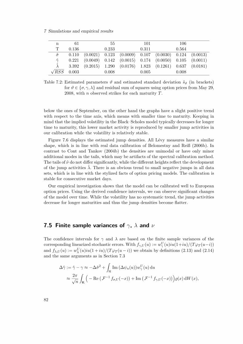
7 Simulations and empirical results
n 61 55 101 106T 0.136 0.233 0.311 0.564σ 0.110 (0.0021) 0.123 (0.0009) 0.107 (0.0030) 0.124 (0.0013)γ 0.221 (0.0049) 0.142 (0.0015) 0.174 (0.0050) 0.105 (0.0011)λ 3.392 (0.2015) 1.290 (0.0176) 1.823 (0.1261) 0.637 (0.0181)√RSS 0.003 0.008 0.005 0.008
Table 7.2: Estimated parameters ϑ and estimated standard deviation sϑ (in brackets)for ϑ ∈ σ, γ, λ and residual sum of squares using option prices from May 29,2008, with n observed strikes for each maturity T .
below the ones of September, on the other hand the graphs have a slight positive trendwith respect to the time axis, which means with smaller time to maturity. Keeping inmind that the implied volatility in the Black–Scholes model typically decreases for longertime to maturity, this lower market activity is reproduced by smaller jump activities inour calibration while the volatility is relatively stable.Figure 7.6 displays the estimated jump densities. All Lévy measures have a similar
shape, which is in line with real data calibration of Belomestny and Reiß (2006b). Incontrast to Cont and Tankov (2004b) the densities are unimodal or have only minoradditional modes in the tails, which may be artifacts of the spectral calibration method.The tails of ν do not differ significantly, while the different heights reflect the developmentof the jump activities λ. There is an obvious trend to small negative jumps in all datasets, which is in line with the stylized facts of option pricing models. The calibration isstable for consecutive market days.Our empirical investigation shows that the model can be calibrated well to European
option prices. Using the derived confidence intervals, we can observe significant changesof the model over time. While the volatility has no systematic trend, the jump activitiesdecrease for longer maturities and thus the jump densities become flatter.
7.5 Finite sample variances of γ, λ and ν
The confidence intervals for γ and λ are based on the finite sample variances of thecorresponding linearized stochastic errors. With fγ,U (u) := wUγ (u)iu(1+iu)/(TϕT (u−i))and fλ,U (u) := wUλ (u)iu(1 + iu)/(TϕT (u− i)) we obtain by definitions (2.13) and (2.14)and the same arguments as in Section 7.3
∆γ := γ − γ ≈ −∆σ2 +∫R
Im(∆ψn(u)
)wUγ (u) du
≈ 2π√n
∫R
(− Re
(F−1 fσ,U (−x)
)+ Im
(F−1 fγ,U (−x)
))%(x) dW (x),
82
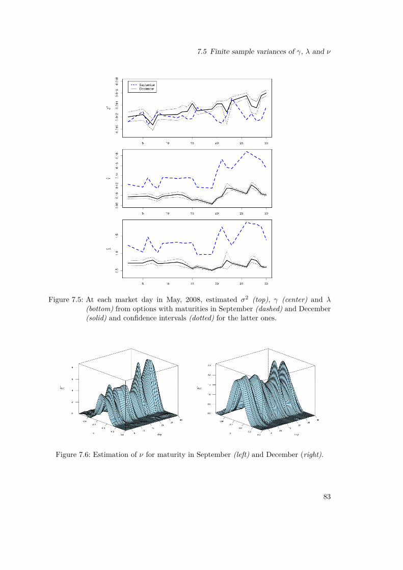
7.5 Finite sample variances of γ, λ and ν
Figure 7.5: At each market day in May, 2008, estimated σ2 (top), γ (center) and λ(bottom) from options with maturities in September (dashed) and December(solid) and confidence intervals (dotted) for the latter ones.
Figure 7.6: Estimation of ν for maturity in September (left) and December (right).
83
7 Simulations and empirical results
∆λ := λ− λ ≈ 12∆σ2 + ∆γ −
∫R
Re(∆ψn(u)
)wUλ (u) du
≈ 2π√n
∫R
(− Re
(12 F−1 fσ,U (−x)
+ F−1 fλ,U (−x))
+ Im(F−1 fγ,U (−x)
))%(x) dW (x).
Therefore, the finite sample variances are given by
s2γ = 4π2
n
∫R
(− Re
(F−1 fσ,U (−x)
)+ Im
(F−1 fγ,U (−x)
))2%2(x) dx, (7.9)
s2λ = 4π2
n
∫R
(− Re
(12 F−1 fσ,U (−x) + F−1 fλ,U (−x)
)+ Im
(F−1 fγ,U (−x)
))2%2(x) dx. (7.10)
The estimator ν(x0), x0 ∈ R, in (7.2) involves ψn(u + i) instead of ψn(u). Hence, theconfidence intervals for ν(x0) are based on the linearization
∆ψn(u+ i) := ψn(u+ i)− ψ(u+ i)
≈ −u(u+ i)TϕT (u) (F On −F O)(u+ i)
≈ − 1√n
u(u+ i)TϕT (u)
∫R
eiux−x%(x) dW (x) =: 1√nLν(u).
Defining fν,U (u) := −wUν (u)u(u + i)/(TϕT (u)) and writing for brevity g(m)U (x0) :=
F−1[umwUν (u)](x0) with m ∈ 0, 1, 2, the dominating stochastic error term of ν(x0)is then given by (cf. (4.3))
∆ν(x0) :=ν(x0)− ν(x0)
≈ 1√n
( 12π
∫R
e−iux0Lν(u)wUν (u) du
+ ∆σ2
2 g(2)U (x0)− i∆γg(1)
U (x0) + ∆λg(0)U (x0)
)≈ 2π√
n
∫R
(e−x2π F
−1fν,U (x0 − x)
+ Re(F−1 fσ,U (−x)
)(12g
(2)U (x0) + ig
(1)U (x0)− 1
2g(0)U (x0)
)+ Im
(F−1 fγ,U (−x)
)(− ig(1)
U (x0) + g(0)U (x0)
)− Re
(F−1 fλ,U (−x)
)g
(0)U (x0)
)%(x) dW (x),
where we note that g(0)U , g
(2)U are purely real and g(1)
U has only an imaginary part by thesymmetry of wUν . Hence, the variance of the linearized stochastic error of ν(x0) is given
84

7.5 Finite sample variances of γ, λ and ν
by
s2ν(x0) =4π2
n
∫R
(e−x2π F
−1fν,U (x0 − x)
+ Re(F−1 fσ,U (−x)
)(12g
(2)U (x0) + ig
(1)U (x0)− 1
2g(0)U (x0)
)+ Im
(F−1 fγ,U (−x)
)(− ig(1)
U (x0) + g(0)U (x0)
)− Re
(F−1 fλ,U (−x)
)g
(0)U (x0)
)2%2(x) dx. (7.11)
85

8 A uniform central limit theorem fordeconvolution estimators
In this chapter, the second problem of this thesis is treated, namely the deconvolutionproblem. Our observations are given by n ∈ N independent and identically distributedrandom variables
Yj = Xj + εj , j = 1, . . . , n, (8.1)
where Xj and εj are independent of each other, the distribution of the errors εj issupposed to be known and the aim is statistical inference on the distribution of Xj .Let us denote the densities of Xj and εj by fX and fε, respectively. The structuralsimilarity of the deconvolution problem and the problem of estimating the characteristictriplet of a Lévy process has been discussed in the introduction and in connection withequation (2.28) in Section 2.2. We consider the case of ordinary smooth errors, whichmeans that the characteristic function ϕε of the errors εj decays with polynomial rate,determining the ill–posedness of the inverse problem. We prove a uniform central limittheorem for kernel estimators of the distribution function of Xj in the setting of
√n
convergence rates. More precisely, the theorem does not only include the estimation ofthe distribution function, but covers estimating translation classes of linear functionalsof the density fX . These results will appear in the paper Söhl and Trabs (2012a), wherein addition lower bounds for the estimators are studied. In the paper, we show that theused estimators are optimal in the sense of semiparametric efficiency.The classical Donsker theorem plays a central role in statistics. Let X1, . . . , Xn be
an independent, identically distributed sample from a distribution function F on thereal line and define the empirical distribution function by Fn(t) := 1
n
∑nj=1 1Xj6t. The
classical Donsker theorem states that√n(Fn − F ) converges in law to G in the space
of bounded functions `∞(R), where G is obtained by the composition of the distribu-tion function F and a standard Brownian bridge. In the deconvolution model (8.1)the random variables X1, . . . , Xn are not observed, but only Y1, . . . , Yn, which con-tain an additive error. In this model we consider estimators ϑt of linear functionalst 7→ ϑt :=
∫ζ(x− t)fX(x) dx, where the special case ζ := 1(−∞,0] leads to the estimation
of the distribution function F . Our Donsker theorem states that√n(ϑt−ϑt)t∈R converges
in law to a centered Gaussian Borel random variable G in `∞(R). This generalizationallows to consider functionals ϑt as long as the smoothness of ζ in an L2–Sobolev sensecompensates the ill–posedness of the problem.In order to show the uniform central limit theorem in the deconvolution problem, we
prove that the empirical process√n(Pn−P) is tight in the space of bounded mappings
87
8 A uniform central limit theorem for deconvolution estimators
acting on the class
G := F−1[1/ϕε(−•)] ∗ ζt| t ∈ R, ζt := ζ(•− t),
where P and Pn = 1n
∑nj=1 δYj denote the true and the empirical probability measure
of the observations Yj , respectively. Since G may consist of translates of an unboundedfunction, this is in general not a Donsker class. Nevertheless, Radulović and Wegkamp(2000) have observed that a smoothed empirical processes might converge even when theunsmoothed process does not. Giné and Nickl (2008) have further developed these ideasand have shown uniform central limit theorems for kernel density estimators. Nickl andReiß (2012) used smoothed empirical processes in the inverse problem of estimating thegeneralized distribution function of Lévy measures.Additionally to techniques of smoothed empirical processes, our proofs rely on the
Fourier multiplier property of the underlying deconvolution operator F−1[1/ϕε], whichis related to pseudo–differential operators as noted in the Lévy process setting by Nickland Reiß (2012) and in the deconvolution context by Schmidt–Hieber et al. (2012).Important for our proofs are the mapping properties of F−1[1/ϕε] on Besov spaces.This chapter is organized as follows: In Section 8.1, we define the estimator. In Sec-
tion 8.2, we formulate the uniform central limit theorem, which we discuss in Section 8.3.Useful properties of the deconvolution operator are collected in Section 8.4. The proofof the uniform central limit theorem is divided into proving the convergence of the finitedimensional distributions in Section 8.5 and tightness in Section 8.6. Definitions andproperties of the function spaces used in this chapter are contained in Section 8.7.
8.1 The estimator
According to the observation scheme (8.1), Yj are distributed with density fY = fX ∗ fεdetermining the probability measure P. Let ϕ and ϕε be the characteristic functionsof the Yj and of the εj , respectively. We define the Fourier transform by F f(u) :=∫eiuxf(x) dx, u ∈ R. On the assumption that ϕε does not vanish, we obtain F fX(u) =
ϕ(u)/ϕε(u). For two different functions fX and fX we denote by ϕ and ϕ, respectively,the characteristic functions of the corresponding observations. We have
F [fX − fX ](u) = ϕ(u)− ϕ(u)ϕε(u) . (8.2)
For ζ to be specified later and recalling ζt = ζ(•− t), our aim is to estimate functionalsof the form
ϑt := 〈ζt, fX〉 =∫ζt(x)fX(x) dx. (8.3)
The characteristic function ϕ of P can be estimated by its empirical version ϕn(u) =1n
∑nj=1 e
iuYj , u ∈ R. Equation (8.2) shows that the difference between two characteristicfunctions ϕ and ϕ will be divided by the decaying function ϕε. So we apply a spectralcut–off by multiplying with the Fourier transform of a band–limited kernel. The natural
88
8.2 Statement of the theorem
estimator of the functional ϑt is given by
ϑt :=∫ζt(x)F−1
[F Kh
ϕnϕε
](x) dx, (8.4)
where K is a band–limited kernel, h > 0 the bandwidth and we have written as usualKh(x) = h−1K(x/h). Choosing F K = 1[−κ,κ] for some κ > 0 leads to the estimatorproposed by Butucea and Comte (2009). Throughout, we suppose that
(i) K ∈ L1(R) ∩ L∞(R) is symmetric and band–limited with supp(F K) ⊆ [−1, 1],
(ii) for l = 1, . . . , L∫K = 1,
∫xlK(x) dx = 0,
∫|xL+1K(x)|dx <∞ and (8.5)
(iii) K ∈ C1(R) satisfies, denoting 〈x〉 := (1 + x2)1/2,
|K(x)|+ |K ′(x)| . 〈x〉−2. (8.6)
Throughout, we write Ap . Bp if there exists a constant C > 0 independent of theparameter p such that Ap 6 CBp. If Ap . Bp and Bp . Ap, we write Ap ∼ Bp.Examples of such kernels can be obtained by taking F K to be a symmetric function inC∞(R) which is supported in [−1, 1] and constant to one in a neighborhood of zero. Theresulting kernels are called flat top kernels and were used in deconvolution problems, forexample, by Bissantz et al. (2007).
8.2 Statement of the theorem
Given a function ζ specified later, our aim is to show a uniform central limit theoremfor the estimator over the class of translations ζt, t ∈ R. In view of the classical Donskertheorem in a model without additive errors, where no assumptions on the smoothness ofthe distribution are needed, we want to assume as less smoothness of fX as possible stillguaranteeing
√n–rates. For some δ > 0 the following assumptions on the density fX will
be needed:
Assumption 8.1.
(i) Let fX be bounded and assume the moment condition∫|x|2+δfX(x) dx <∞.
(ii) Assume fX ∈ Hα(R) that is the density has Sobolev smoothness of order α > 0.
We refer to the appendix for an exact definition of the Sobolev spaceHα(R). Bounded-ness of the observation density fY follows immediately from point (i) of the assumptionsince ‖fY ‖∞ 6 ‖fX‖∞‖fε‖L1 <∞. In addition to the smoothness of fX , the smoothness
89
8 A uniform central limit theorem for deconvolution estimators
of ζ will be crucial. We assume for γs, γc > 0
ζ ∈ Zγs,γc :=ζ =ζc + ζs
∣∣∣ζs ∈ Hγs(R) is compactly supported as well
as 〈x〉τ(ζc(x)− a(x)
)∈ Hγc(R) for some τ > 0 and (8.7)
some a ∈ C∞(R) such that a′ is compactly supported
and write for ζ ∈ Zγs,γc with a given decomposition ζ = ζs + ζc
‖ζ‖Zγs,γc := ‖ζs‖Hγs +∥∥ 1ix+1ζ
c(x)∥∥Hγc
,
which is finite since the second term ‖ 1ix+1ζ
c(x)‖Hγc can be bounded by ‖ a(x)ix+1‖Hγc +
‖ 1(ix+1)〈x〉τ ‖Cs‖〈x〉
τ (ζc(x) − a(x))‖Hγc < ∞ for any s > γc. Let us give two examplesfor ζ and corresponding γs, γc.
Example 8.2. To estimate the distribution function of Xj , one has to consider trans-lations of the indicator function 1(−∞,0](x), x ∈ R. Let a be a monotone decreasingC∞(R) function, which is for some M > 0 equal to zero for all x >M and equal to onefor all x 6 −M . We define ζs := 1(−∞,0] − a and ζc := a. From the bounded variationof ζs follows ζs ∈ B1
1,∞(R) ⊆ Hγs(R) for any γs < 1/2 by Besov smoothness of boundedvariation functions (8.38) as well as by the Besov space embeddings (8.33) and (8.34).Since a ∈ C∞(R) and a′ is compactly supported, the condition on ζc is satisfied for anyγc > 0. Hence, 1(−∞,t] ∈ Zγs,γc if γs < 1/2. On the other hand, this cannot hold forγs > 1/2 since Hγs(R) ⊆ C0(R) by Sobolev’s embedding theorem or by (8.32), (8.33)and (8.34).
Example 8.3. In the context of M–estimation (or Z–estimation) the root of the equation
〈ζ(· − t), fX〉 = 0
is used for inference, e.g., on the location of the distribution of Xj . A popular examplein robust statistics is the Huber estimator where ζ(x) = hK(x) := ((−K) ∨ x) ∧K forsome K > 0. In that case a similar decomposition as in Example 8.2 shows hK ∈ Zγs,γcfor any γs < 3/2.
The ill–posedness of the problem is determined by the decay of the characteristicfunction of the errors. More precisely, we suppose
Assumption 8.4. Let the error distribution satisfy
(i)∫|x|2+δfε(x) dx <∞ thus ϕε is twice continuously differentiable and
(ii) |(ϕ−1ε )′(u)| . 〈u〉β−1 for some β > 0, in particular |ϕ−1
ε (u)| . 〈u〉β, u ∈ R.
Throughout, we write ϕ−1ε = 1/ϕε. The Assumption (ii) on the distribution of the errors
is similar to the classical decay assumption by Fan (1991a) and it is fulfilled for many
90
8.2 Statement of the theorem
ordinary smooth error laws such as gamma or Laplace distributions as discussed below.Assumption 8.4(ii) implies that ϕ−1
ε is a Fourier multiplier on Besov spaces so that
Bsp,q(R) 3 f 7→ F−1[ϕ−1
ε (−•)F f ] ∈ Bs−βp,q (R)
for p, q ∈ [1,∞], s ∈ R, is a continuous linear map, which is essential in our proofs,compare Lemma 8.8. In the same spirit Schmidt–Hieber et al. (2012) discuss the behaviorof the deconvolution operator as pseudo–differential operator. We define
gt := F−1[ϕ−1ε (−•)] ∗ ζt and G = gt|t ∈ R. (8.8)
Note that in general gt may only exist in a distributional sense, but on Assumption 8.4and for ζ ∈ Zγs,γc it can be rigorously interpreted by (see (8.17))
g0(x) =F−1[ϕ−1ε (−u)F ζs(u)](x)
+ (1 + ix)F−1[ϕ−1ε (−u)F [ 1
iy+1ζc(y)](u)](x)
+ F−1[(ϕ−1ε )′(−u)F [ 1
iy+1ζc(y)](u)](x),
which indicates why we have imposed an assumption on (ϕ−1ε )′ and have defined ‖•‖Zγs,γc
as above.It will turn out that G is P–pregaussian, but not Donsker in general. Denoting by bαc
the largest integer smaller or equal to α and defining convergence in law on `∞(R) asDudley (1999, p. 94), we state our main result
Theorem 8.5. Grant Assumptions 8.1 and 8.4 as well as ζ ∈ Zγs,γc with γs > β, γc >(1/2 ∨ α) + γs and α + 3γs > 2β + 1. Furthermore, let the kernel K satisfy (8.5) withL = bα+ γsc. Let h2α+2γs
n n→ 0 and if γs 6 β + 1/2 let in addition hρnn→∞ for someρ > 4β − 4γs + 2, then
√n(ϑt − ϑt)t∈R
L−→ G in `∞(R)
as n → ∞, where G is a centered Gaussian Borel random variable in `∞(R) with co-variance function given by
Σs,t :=∫gs(x)gt(x)P( dx)− ϑsϑt
for gs, gt defined in (8.8) and s, t ∈ R.
We illustrate the range of this theorem by the following examples.
Example 8.6. For estimating the distribution function Assumption 8.4 needs to befulfilled for some β < 1/2 owing to the condition γs > β. This is fulfilled by the gammadistribution Γ(β, η) with β ∈ (0, 1/2) and η ∈ (0,∞), that is
fε(x) := γβ,η(x) := 1Γ(β)ηβ x
β−1e−x/η1[0,∞)(x), x ∈ R,
91
8 A uniform central limit theorem for deconvolution estimators
and ϕε(u) = (1− iηu)−β, u ∈ R.For the Huber estimator from Example 8.3 we required β < 3/2, which holds, for
instance, for the chi–squared distribution with one or two degrees of freedom or for theexponential distribution.
Example 8.7. Butucea and Comte (2009) studied the case β > 1 and derived√n–
rates for γs > β in our notation. In particular, they considered supersmooth ζ, that isF ζ decays exponentially. In this case ζ ∈ Hs(R) for any s ∈ N. Requiring the slightlystronger assumption that 〈x〉τζ(x) ∈ Hs(R) for some arbitrary small τ > 0 and for alls ∈ N we can choose ζc := ζ and ζs := 0. Then β can be taken arbitrary large suchthat all gamma distributions, the Laplace distributions and convolutions of them can bechosen as error distributions.
8.3 Discussion
To have√n–rates we suppose γs > β in Theorem 8.5, which means that the smooth-
ness of the functionals compensates the ill–posedness of the problem. This condition isnatural in view of the abstract analysis in terms of Hilbert scales by Goldenshluger andPereverzev (2003), who obtain the minimax rate n−(α+γs)/(2α+2β) ∨ n−1/2 in our nota-tion. As a consequence of the condition on γs and γc we can bound the stochastic errorterm of the estimator ϑt uniformly in h ∈ (0, 1). The bias term is of order hα+γs .For γs > β + 1/2 the class G is a Donsker class. In this case the only condition on the
bandwidth is that the bias tends faster than n−1/2 to zero. In the interesting but involvedcase γs ∈ (β, β + 1/2], the class G will in general not be a Donsker class. Estimating thedistribution function as in Example 8.2 belongs to this case. In order to see that G isin general not a Donsker class, let the error distribution be given by fε = γβ,η(−•) andζ = γσ,η with σ ∈ (γs + 1/2, β + 1). Then gt equals γσ−β,η ∗ δt. For the shape parameterholds σ − β ∈ (1/2, 1) and thus gt is an L2(R)–function unbounded at t. The Lebesguedensity of P is bounded by Assumption 8.1(i). Hence, G consists of all translates of anunbounded function and thus cannot be Donsker, cf. Theorem 7 by Nickl (2006).Therefore, for γs ∈ (β, β+ 1/2] smoothed empirical processes are necessary, especially
we need to ensure enough smoothing to be able to obtain a uniform central limit theorem.The bandwidth cannot tend too fast to zero, more precisely we require hρnn→∞ as n→∞ for some ρ with ρ > 4β−4γs+2. In combination with the bias condition h2α+2γs
n n→ 0as n → ∞ we obtain necessarily α + γs > 2β − 2γs + 1 leading to the assumption inthe theorem. Since 2α + 2γs > α + 2β − γs + 1 > 4β − 4γs + 2 we can always choosehn ∼ n−1/(α+2β−γs+1). In contrast to Butucea and Comte (2009); Dattner et al. (2011);Fan (1991b) our choice of the bandwidth hn is not determined by the bias–variance trade–off, but rather by the amount of smoothing necessary to obtain a uniform central limittheorem. The classical bandwidth hn ∼ n−1/(2α+2β) is optimal for estimating the densityin the sense that it achieves the minimax rate with respect to the mean integrated squarederror (MISE), compare Fan (1991b) who assumes Hölder smoothness of fX instead ofL2–Sobolev smoothness. For this choice the bias condition h2α+2γs
n n → 0 is satisfied.
92
8.3 Discussion
If γs 6 β + 1/2 the classical bandwidth satisfies the additional minimal smoothnesscondition in the case of estimating the distribution function with mild conditions onfX . It suffices for example that fX is of bounded variation. Then α and γs can bechosen large enough in (0, 1/2) such that 2α + 2β > 4β − 4γs + 2 and the classicalbandwidth satisfies the conditions of the theorem. Whenever the classical bandwidthhn ∼ n−1/(2α+2β) satisfies the conditions of Theorem 8.5, then the corresponding densityestimator is a ‘plug–in’ estimator in the sense of Bickel and Ritov (2003) meaning thatthe density is estimated rate optimal for the MISE and the estimators of the functionalsconverge uniformly over t ∈ R.The smoothness condition on the density fX is then a consequence of the given choice
of hn together with the classical bias estimate for kernel estimators. As we have seen inExample 8.2 for estimating the distribution function, we have ζ = 1(−∞,0] ∈ Zγs,γc withγs < 1/2 arbitrary close to 1/2. In the classical Donsker theorem which correspondsto the case β → 0 the condition α + 3γs > 2β + 1 would simplify to α > −1/2.However, we suppose fX to be bounded, which leads to much clearer proofs, and thusfX ∈ H0(R) is automatically satisfied. Assumption 8.1 allows to focus on the interplaybetween the functional ζ and the deconvolution operator F−1[ϕ−1
ε ]. Nickl and Reiß(2012) have studied the case of unbounded densities, which is necessary in the Lévyprocess setup, but considered ζt = 1(−∞,t] only. The class Zγs,γc is defined by L2–Sobolevconditions so that bounded variation arguments for ζ have to be avoided in the proofs.An interesting aspect is the following: If we restrict the uniform convergence to (ζt)t∈T
for some compact set T ⊆ R, it is sufficient to assume 1ix+1ζ
c ∈ Hγc(R) instead ofrequiring (1∨|x|τ )(ζc(x)−a(x)) ∈ Hγc(R) for some τ > 0 and a function a ∈ C∞(R) suchthat a′ is compactly supported as done in Zγs,γc . In particular, slowly growing ζ wouldbe allowed. The stronger condition in the definition of Zγs,γc is only needed to ensurepolynomial covering numbers of gt|t ∈ T for T ⊆ R unbounded (cf. Theorem 8.10below).As a corollary of Theorem 8.5 we can weaken Assumption 8.4(ii). If the characteristic
function of the errors ε is given by ϕε = ϕεψ where ϕε satisfies Assumption 8.4(ii) andthere is a Schwartz distribution ν ∈ S ′(R) such that F ν = ψ−1 and ν ∗ ζ ∈ Zγs,γc forζ ∈ Zγs,γc , then for t ∈ R
F−1[ϕ−1ε ] ∗ ζ(•− t) = F−1[ϕ−1
ε ] ∗ (ν ∗ ζ)(•− t)
and thus we can proceed as before. For instance, for translated errors fε ∗ δµ withµ 6= 0, the distribution ν would be given by δ−µ. Thus even if ϕε does not satisfyAssumption 8.4(ii) the statement of Theorem 8.5 holds true if we can write ϕε(u) =ϕε(u)eiµu with ϕε satisfying Assumption 8.4(ii). The assumption by Fan and Liu (1997)for the asymptotic normality in the case of ordinary smooth deconvolution are weakerthan the assumptions by Fan (1991a) since they allow exactly for this additional factoreiµu in the assumptions on the characteristic function of the error.As for the classical Donsker theorem the Donsker theorem for deconvolution estimators
has many different applications, the most obvious being the construction of confidencesets. Further Donsker theorems may be obtained by applying the functional delta method
93
8 A uniform central limit theorem for deconvolution estimators
to Hadamard differentiable maps.In order to construct confidence intervals or joint confidence sets at finitely many
points we take m different points t1, . . . , tm ∈ R. Let the assumptions of Theorem 8.5be fulfilled. Then gt ∈ L2(P) for all t ∈ R and Σs,t =
∫gs(x)gt(x)Pn( dx) − ϑsϑt is a
consistent estimator of the covariance Σs,t =∫gs(x)gt(x)P( dx)− ϑsϑt by the weak law
of large numbers. The spectral theorem yields an orthogonal matrix O and a diagonalmatrix D such that the covariance matrix Σ corresponding to the points t1, . . . , tm ∈ Rcan be written as Σ = ODO>. We assume that the determinant of Σ is nonzero andthus the diagonal entries of D are positive. By the convergence of the finite dimensionaldistributions we have
√n
ϑt1 − ϑt1
...ϑtm − ϑtm
d−→ X, (8.9)
where X ∼ N(0,Σ). The distribution of X is the same as the distribution of OD1/2Yfor a random vector Y of m independent standard normal random variables. By thecontinuous mapping theorem we can apply the map (OD1/2)−1 to (8.9). Let kη denotethe (1 − η)–quantile of the chi–squared distribution χ2
m of m degrees of freedom. Wedefine
An := (ϑt1 , . . . , ϑtm)> + n−1/2OD1/2 x ∈ Rm | ‖x‖ 6 kη ,
where ‖x‖ denotes the Euclidean norm. Then we have the following confidence statement
limn→∞
P((ϑt1 , . . . , ϑtm) ∈ An) = 1− η.
The special case m = 1 yields confidence intervals.Let us illustrate the construction of confidence bands. By the continuous mapping
theorem we infer
supt∈R
√n|ϑt − ϑt|
L−→ supt∈R|G(t)|.
The construction of confidence bands reduces now to knowledge about the distributionof the supremum of G. Suprema of Gaussian processes are well studied and informationabout their distribution can be either obtained from theoretical considerations as invan der Vaart and Wellner (1996, App. A.2) or from Monte Carlo simulations. Let q1−ηbe the (1− η)–quantile of supt∈R |G(t)| that is P(supt∈R |G(t)| 6 q1−η) = 1− η. Then
limn→∞
P(ϑt ∈ [ϑt − q1−ηn
−1/2, ϑt + q1−ηn−1/2] for all t ∈ R
)= 1− η
and thus the intervals [ϑt − q1−ηn−1/2, ϑt + q1−ηn
−1/2] define a confidence band.As often in the literature we assume the error distribution to be known. In a more
realistic setting where an independent sample of pure noise observations is observable,
94
8.4 The deconvolution operator
Neumann (1997) constructs a density estimator for unknown errors. In this case thedeconvolution operator F−1[ϕ−1
ε ] needs to be estimated leading to an inverse problemwith an error in the operator. A Donsker theorem in this situation is related to the Lévyprocess setting of Nickl and Reiß (2012) since their estimator is based on the deconvolu-tion with the unknown marginal distribution of the process. Another interesting aspectis the similarity of the deconvolution problem and the errors–in–variables regression,see for example Fan and Truong (1993) and the references therein. The correspondingstatement to our result would be a uniform central limit theorem for linear functionalsof the regression function, where similar methods may be applied.
8.4 The deconvolution operatorIn this section, we provide an auxiliary lemma, which describes the properties of thedeconvolution operator F−1[ϕ−1
ε ].
Lemma 8.8. Grant Assumption 8.4.
(i) For all s ∈ R, p, q ∈ [1,∞] the deconvolution operator F−1[ϕ−1ε (−•)] is a Fourier
multiplier from Bsp,q(R) to Bs−β
p,q (R), that is the linear map
Bsp,q(R)→ Bs−β
p,q (R), f 7→ F−1[ϕ−1ε (−•)F f ]
is bounded.
(ii) For any integer m strictly larger then β we have F−1[(1 + iu)−mϕ−1ε ] ∈ L1(R) and
if m > β + 1/2 we also have F−1[(1 + iu)−mϕ−1ε ] ∈ L2(R).
(iii) Let β+ > β and f, g ∈ Hβ+(R). Then∫ (F−1[ϕ−1
ε ] ∗ f)g =
∫ (F−1[ϕ−1
ε (−•)] ∗ g)f. (8.10)
Using the kernel K, this equality extends to functions g ∈ L2(R) ∪ L∞(R) andfinite Borel measures µ:∫ (
F−1[ϕ−1ε F Kh] ∗ µ
)g =
∫ (F−1[ϕ−1
ε (−•)F Kh] ∗ g)
dµ. (8.11)
Proof.
(i) Analogously to the proof by Nickl and Reiß (2012), we deduce from Corollary 4.11of Girardi andWeis (2003) that (1+iu)−βϕ−1
ε (−u) is a Fourier multiplier on Bsp,q by
Assumption 8.4(ii). It remains to note that j : Bsp,q(R)→ Bs−β
p,q (R), f 7→ F−1[(1 +iu)β F f ] is a linear isomorphism (Triebel, 2010, Thm. 2.3.8).
(ii) Since the gamma density γ1,1 is of bounded variation, it is contained in B11,∞(R)
by (8.38). Using the isomorphism j from (i), we deduce γm,1 ∈ Bm1,∞(R) and thus
95
8 A uniform central limit theorem for deconvolution estimators
by Besov embeddings (8.34) and (8.31)
F−1[(1 + iu)−mϕ−1ε ] ∈ Bm−β
1,∞ (R) ⊆ B01,1(R) ⊆ L1(R).
If m− β > 1/2, we can apply the embedding Bm−β1,∞ (R) ⊆ Bm−β−1/2
2,∞ (R) ⊆ L2(R).
(iii) For f ∈ Hβ+(R), (i) and the Besov embeddings (8.31), (8.33) and (8.34) yield
‖F−1[ϕ−1ε ] ∗ f‖L2 . ‖F−1[ϕ−1
ε ] ∗ f‖B02,1
. ‖f‖Bβ2,1
. ‖f‖Hβ+ <∞.
Therefore, it follows by Plancherel’s equality∫ (F−1[ϕ−1
ε ] ∗ f)(x)g(x) dx = 1
2π
∫ϕ−1ε (−u)F f(−u)F g(u) du
=∫ (F−1[ϕ−1
ε (−•)] ∗ g)(x)f(x) dx.
To prove the second part of the claim for g ∈ L2(R), we note that by Young’sinequality
‖F−1[ϕ−1ε F Kh]‖L2 6 ‖F−1[ϕ−1
ε 1[−1/h,1/h]]‖L2‖Kh‖L1 <∞
due to the support of F K and Assumption (8.6) on the decay of K. Since µ is afinite measure and g is bounded, Fubini’s theorem yields then∫
g(x)(F−1[ϕ−1
ε F Kh] ∗ µ)(x) dx
=∫ ∫
g(x)F−1[ϕ−1ε F Kh](x− y)µ( dy) dx
=∫ (F−1[ϕ−1
ε (−•)F Kh] ∗ g)(y)µ( dy),
where we have used the symmetry of the kernel. In order to apply Fubini’s theoremfor the case g ∈ L∞(R), too, we have to show that ‖F−1[ϕ−1
ε F Kh]‖L1 is finite.We replace the indicator function by a function χ ∈ C∞(R) which equals one on[−1/h, 1/h] and is compactly supported. We estimate
‖F−1[ϕ−1ε F Kh]‖L1 6 ‖F−1[ϕ−1
ε χ]‖L1‖Kh‖L1 . (8.12)
Using that ϕ−1ε χ is twice continuously differentiable and has got compact support,
we obtain
‖(1 + x2)F−1[ϕ−1ε χ](x)‖∞ 6 ‖F−1[(Id−D2)ϕ−1
ε χ](x)‖∞6 ‖(Id−D2)ϕ−1
ε χ‖L1 <∞,
where we denote the identity and the differential operator by Id and D, respectively.
96
8.5 Convergence of the finite dimensional distributions
This shows that (8.12) is finite.
8.5 Convergence of the finite dimensional distributions
As usual, we decompose the error into a stochastic error term and a bias term:
ϑt − ϑt = ϑt − E[ϑt] + E[ϑt]− ϑt
=∫ζt(x)F−1
[F Kh
ϕn − ϕϕε
](x) dx+
∫ζt(x)(Kh ∗ fX(x)− fX(x)) dx.
8.5.1 The bias
The bias term can be estimated by the standard kernel estimator argument. Let usconsider the singular and the continuous part of ζ separately. Applying Plancherel’sidentity and Hölder’s inequality, we obtain∣∣∣∣∫ ζst (x)(Kh ∗ fX(x)− fX(x)) dx
∣∣∣∣= 1
2π
∣∣∣∣∫ F ζst (u)(F K(hu)− 1)F fX(−u) du∣∣∣∣
6 ‖〈u〉−(α+γs)(F K(hu)− 1)‖∞∫〈u〉α+γs | F ζs(u)F fX(u)|du
6 hα+γs‖u−(α+γs)(F K(u)− 1)‖∞‖ζs‖Hγs‖fX‖Hα .
The term ‖u−(α+γs)(F K(u)−1)‖∞ is finite using the a Taylor expansion of F K aroundzero with (F K)(l) = 0 for l = 1, . . . , bα+ γsc by the order of the kernel (8.5).For the smooth part of ζt Plancherel’s identity yields∣∣∣∣∫ ζct (x)(Kh ∗ fX − fX)(x) dx
∣∣∣∣= 1
2π
∣∣∣∣∫ F [ 1ix+1ζ
ct (x)](Id + D)(F K(hu)− 1)F fX(−u) du
∣∣∣∣6∫| F [ 1
ix+1ζct (x)](F K(hu)− 1 + hF [ixK](hu))F fX(−u)|du
−∫| F [ 1
ix+1ζct (x)](F K(hu)− 1)F [ixfX ](−u)|du.
The first term can be estimated as before and for the second term we note that xfX(x) ∈L2(R) = H0(R) by Assumption 8.1(i) such that the additional smoothness of 1
ix+1ζc(x)
yields the right order. Therefore, we have |E[ϑt] − ϑt| . hα+γs and thus by the choiceof h, the bias term is of order o(n−1/2).
97
8 A uniform central limit theorem for deconvolution estimators
8.5.2 The stochastic error
We notice that ‖ζc − a‖Hγc . ‖〈x〉−τ‖Cs‖〈x〉τ (ζc(x) − a(x))‖Hγc < ∞ for any s > γc,where we used the pointwise multiplier property (8.35) as well as the Besov embeddings(8.34) and (8.32). We have ζs ∈ L2 and by (8.31), (8.33) and (8.34)
‖ζc‖∞ 6 ‖a‖∞ + ‖ζc − a‖∞ 6 ‖a‖∞ + ‖ζc − a‖Hγc <∞,
since γc > 1/2. Consequently, we can apply the smoothed adjoint equality (8.11) andobtain for the stochastic error term∫
ζt(x)F−1[F Kh
ϕn − ϕϕε
](x) dx
=∫F−1[ϕ−1
ε (−•)F Kh] ∗ ζt(x)(Pn−P)( dx). (8.13)
Therefore, it suffices for the convergence of the finite dimensional distributions to boundthe term
suph∈(0,1)
∫ ∣∣∣F−1[ϕ−1ε (−•)F Kh] ∗ ζ(x)
∣∣∣2+δP( dx), (8.14)
for any function ζ ∈ Zγs,γc . Then the stochastic error term converges in distribution toa normal random variable by the central limit theorem under the Lyapunov condition(i.e., Klenke, 2007, Thm. 15.43 together with Lem. 15.41). Finally, the Cramér–Wolddevice yields the convergence of the finite dimensional distributions in Theorem 8.5.
First, note that the moment conditions in Assumptions 8.1 and 8.4 and the estimate
|x|pfY (x) 6∫|x− y + y|pfX(x− y)fε(y) dy . (|y|pfX) ∗ fε + fX ∗ (|y|pfε),
for x ∈ R, p > 1, yield finite (2 + δ)th moments for P since∫|x|2+δfY (x) dx . ‖|x|2+δfX‖L1‖fε‖L1 + ‖fX‖L1‖|x|2+δfε‖L1 <∞. (8.15)
To estimate (8.14), we rewrite
F−1[ϕ−1ε (−•)] ∗ ζc(x) = F−1 [ϕ−1
ε (−u)(Id + D)F [ 1iy+1ζ
c(y)](u)](x)
= F−1 [ϕ−1ε (−u)F [ 1
iy+1ζc(y)](u)
](x)
+ F−1 [ϕ−1ε (−u)
(F [ 1
iy+1ζc(y)]
)′(u)](x) (8.16)
= (1 + ix)F−1[ϕ−1ε (−u)F [ 1
iy+1ζc(y)](u)](x)
+ F−1[(ϕ−1ε )′(−u)F [ 1
iy+1ζc(y)](u)](x),
98
8.5 Convergence of the finite dimensional distributions
owing to the product rule for differentiation. Hence,
F−1[ϕ−1ε (−•)] ∗ ζ(x) =F−1[ϕ−1
ε (−u)F ζs(u)](x)+ (1 + ix)F−1[ϕ−1
ε (−u)F [ 1iy+1ζ
c(y)](u)](x)
+ F−1[(ϕ−1ε )′(−u)F [ 1
iy+1ζc(y)](u)](x). (8.17)
While F−1[ϕ−1ε (−•)] ∗ ζ may exist only in distributional sense in general, it is defined
rigorously through the right–hand side of the above display for ζ ∈ Zγs,γc . Consideringζ ∗Kh instead of ζ, we estimate separately all three terms in the following.
The continuity and linearity of the Fourier multiplier F−1[ϕ−1ε (−•)], which was shown
in Lemma 8.8(i), yield for the first term in (8.17)
‖F−1[ϕ−1ε (−u)F ζs(u)F Kh(u)]‖Hδ =
∥∥F−1 [ϕ−1ε (−•)F [ζs ∗Kh]
]∥∥Bδ2,2
. ‖ζs ∗Kh‖Bβ+δ2,2
. ‖ζs‖Hβ+δ ,
where the last inequality holds by ‖F Kh‖∞ 6 ‖K‖L1 . Using the boundedness of fY andthe continuous Sobolev embedding Hδ/4(R) ⊆ L2+δ(R) by (8.31), (8.34) and (8.33), weobtain
‖F−1[ϕ−1ε (−u)F ζs(u)F Kh(u)]‖L2+δ(P)
. ‖F−1[ϕ−1ε (−u)F ζs(u)F Kh(u)]‖L2+δ
. ‖F−1[ϕ−1ε (−u)F ζs(u)F Kh(u)]‖Hδ
. ‖ζs‖Hβ+δ (8.18)
To estimate the second term in (8.17), we use the Cauchy–Schwarz inequality and As-sumption 8.4(ii):
‖F−1[ϕ−1ε (−u)F [ 1
ix+1ζc(x)](u)F Kh(u)]‖∞
6 ‖ϕ−1ε (−u)F [ 1
ix+1ζc]F Kh(u)‖L1
. ‖〈u〉−1/2−β−δϕ−1ε (−u)‖L2‖〈u〉1/2+β+δ F [ 1
ix+1ζc(x)]‖L2
. ‖ 1ix+1ζ
c(x)‖H1/2+β+δ .
Thus∫
(1 + x2)(2+δ)/2fY (x) dx <∞ from (8.15) yields
‖(1 + ix)F−1[ϕ−1ε (−u)F [ 1
iy+1ζc(y)](u)F Kh(u)](x)‖L2+δ(P)
. ‖ 1ix+1ζ
c(x)‖H1/2+β+δ . (8.19)
The last term in the decomposition (8.17) can be estimated similarly using the Cauchy–
99
8 A uniform central limit theorem for deconvolution estimators
Schwarz inequality and Assumption 8.4(ii) for (ϕ−1)′
‖F−1[(ϕ−1ε )′(−u)F [ 1
ix+1ζc(x)](u)F Kh(u)]‖L2+δ(P)
. ‖(ϕ−1ε )′(−u)F [ 1
ix+1ζc(x)](u)‖L1
6 ‖〈u〉1/2−β−δ(ϕ−1ε )′‖L2‖〈u〉−1/2+β+δ F−1[ 1
ix+1ζc(x)](u)‖L2
. ‖ 1ix+1ζ
c(x)‖H−1/2+β+δ . (8.20)
Combining (8.18), (8.19) and (8.20), we obtain
suph∈(0,1)
‖F−1[ϕ−1ε (−•)F Kh] ∗ ζ(x)‖L2+δ(P) . ‖ζ‖Zβ+δ,1/2+β+δ , (8.21)
which is finite for δ small enough satisfying β+ δ 6 γs and 1/2 +β+ δ 6 γc. Since F Kh
converges pointwise to one and | F−1[ϕ−1ε (−•)F Kh] ∗ ζ(x)|2 is uniformly integrable by
the bound of the (2 + δ)th moments, the variance converges to∫ ∣∣∣F−1[ϕ−1ε (−•)] ∗ ζ(x)
∣∣∣2 P( dx).
8.6 TightnessMotivated by the representation (8.13) of the stochastic error, we introduce the empiricalprocess
νn(t) :=√n
∫F−1[ϕ−1
ε (−•)F Kh] ∗ ζt(x)(Pn−P)( dx), t ∈ R . (8.22)
In order to show tightness of the empirical process, we first show some properties of theclass of translations H := ζt|t ∈ R for ζ ∈ Zγs,γc .
Lemma 8.9. For ζ ∈ Zγs,γc the following is satisfied:
(i) The decomposition ζt = ζct + ζst satisfies the conditions in the definition of Zγs,γcwith at. We have supt∈R ‖ζt‖Zγs,γc <∞.
(ii) For any η ∈ (0, γs), there exists τ > 0 such that ‖ζt− ζs‖Zγs−η,γc−η . |t− s|τ holdsfor all s, t ∈ R with |t− s| 6 1.
Proof.
(i) Since ‖ζst ‖2Hγs =∫〈u〉2γs |eituF ζs(u)|2 du = ‖ζs‖2Hγs , both claims hold for the
singular part. Applying the pointwise multiplier property of Besov spaces (8.35) aswell as the Besov embeddings (8.34) and (8.32), we obtain for some M > γc anda ∈ C∞(R) as in definition (8.7)
‖〈x〉τ(ζct (x)− at(x)
)‖Hγc . ‖ 〈x〉
τ
〈x−t〉τ ‖CM ‖〈x− t〉τ (ζct (x)− at(x)
)‖Hγc
= ‖ 〈x〉τ
〈x−t〉τ ‖CM ‖〈x〉τ (ζc(x)− a(x)
)‖Hγc ,
100

8.6 Tightness
which is finite for all t ∈ R since 〈x〉τ 〈x− t〉−τ ∈ CM (R). For the second claim weestimate similarly
supt∈R‖ 1ix+1ζ
ct (x)‖Hγc . sup
t∈R‖at(x)ix+1‖Hγc + ‖ 1
ix+1‖CM supt∈R‖ζct − at‖Hγc
. ‖ 1ix+1‖Hγc‖a‖CM + ‖ 1
ix+1‖CM ‖ζc − a‖Hγc <∞.
(ii) For the singular part note that
‖ζst − ζss‖Hγs−η
6 ‖〈u〉γs F ζs(u)‖L2‖〈u〉−η(1− ei(t−s)u)‖∞. ‖〈u〉−η‖L∞(R \(−|t−s|−1/2,|t−s|−1/2))
∨ ‖(1− ei(t−s)u)‖L∞((−|t−s|−1/2,|t−s|−1/2))
. |t− s|η/2 ∨ |t− s|1/2.
For ζc we have∥∥∥ 1ix+1(ζct (x)− ζcs(x))
∥∥∥Hγc−η
.∥∥∥ 1ix+1ζ
ct (x)−
( 1ix+1ζ
ct (x)
)∗ δs−t
∥∥∥Hγc−η
+∥∥∥ 1i(x−s+t)+1ζ
cs(x)− 1
ix+1ζcs(x)
∥∥∥Hγc−η
.
The first term can be treated analogously to ζs. Using some integerM ∈ N strictlylarger than γc, the second term can be estimated by∥∥∥ 1
i(x−s+t)+1ζcs(x)− 1
ix+1ζcs(x)
∥∥∥Hγc−η
. |t− s|∥∥∥ 1i(x−s+t)+1
1ix+1ζ
cs(x)
∥∥∥Hγc−η
. |t− s|∥∥∥ 1i(x−s+t)+1
∥∥∥CM
∥∥∥ 1ix+1ζ
cs(x)
∥∥∥Hγc−η
. |t− s|,
where we used again pointwise multiplier (8.35), embedding properties of Besovspaces (8.34) and (8.32) as well as (i).
8.6.1 Pregaussian limit processLet G be the stochastic process from Theorem 8.5. It induces the intrinsic covariancemetric d(s, t) := E[(Gs −Gt)2]1/2.
Theorem 8.10. There exists a version of G with uniformly d–continuous sample pathsalmost surely and with supt∈R |Gt| <∞ almost surely.
The proof of the theorem shows in addition that R is totally bounded with respectto d. The boundedness of the sample paths follows from the totally bounded index setand the uniform continuity. Further we conclude that G defined in (8.8) is P–pregaussian
101
8 A uniform central limit theorem for deconvolution estimators
by van der Vaart and Wellner (1996, p. 89). Thus G is a tight Borel random variable in`∞(R) and the law of G is uniquely defined through the covariance structure and thesample path properties in the theorem (van der Vaart and Wellner, 1996, Lem. 1.5.3).
Proof. To show that the class is pregaussian, it suffices to verify polynomial coveringnumbers. To that end, we deduce that
d(s, t) =(‖gt − gs‖2L2(P) − 〈ζt − ζs, fX〉
2)1/2 6 ‖gt − gs‖L2(P) (8.23)
decreases polynomial for |t− s| → 0, for max(s, t)→ −∞ and for min(s, t)→∞. Usingthe same estimates which show the moment bound (8.21) but replacing F Kh = 1, weobtain
‖F [ϕ−1ε (−•)] ∗ ζ‖L2(P) . ‖ζ‖Zβ+δ,1/2+β+δ (8.24)
and thus by choosing δ and η small enough Lemma 8.9 yields the bound d(s, t) .‖ζt − ζs‖Zβ+δ,1/2+β+δ . |t − s|τ . We now turn to the estimation of the tails. We willonly consider the case s, t > N since the case s, t 6 N can be treated in the same way.Without loss of generality, let s < t.For the smooth component of ζ we have to show that
∥∥ 1ix+1(ζct (x) − ζcs(x))
∥∥Hγc
witht, s > N decays polynomially in N . It suffices to prove
∥∥ 1ix+1(ζct − at)(x)
∥∥Hγc
and∥∥ 1ix+1(at − as)(x)
∥∥Hγc
with a ∈ C∞(R) from definition (8.7) of Zγs,γc both decay poly-nomially in N . Let M > γc and ψ ∈ CM (R) with ψ(x) = 1 for x ∈ R \[−1
2 ,12 ] and
ψ(x) = 0 for x ∈ [−14 ,
14 ]. The pointwise multiplier property (8.35) yields∥∥ 1
ix+1(ζct − at)(x)∥∥Hγc
=∥∥(ψ(x/N) + (1− ψ(x/N))
) 1ix+it+1(ζc − a)(x)
∥∥Hγc
. ‖ 1ix+it+1‖CM ‖ψ(x/N)(ζc − a)(x)‖Hγc + ‖1−ψ(x/N)
ix+it+1 ‖CM ‖ζc − a‖Hγc
. ‖〈x〉−τψ(x/N)‖CM ‖〈x〉τ (ζc − a)(x)‖Hγc +N−1‖ζc − a‖Hγc
. N−(τ∧1)
and for N large enough such that supp(a′) ⊆ [−N/2, N/2] we obtain∥∥ 1ix+1(at − as)(x)
∥∥Hγc
=∥∥ψ(x/N)
ix+1 (at − as)(x)∥∥Hγc
.∥∥ψ(x/N)
ix+1∥∥Hγc
∥∥(at − as)(x)∥∥CM
.∥∥(ix+ 1)−3/4∥∥
Hγc
∥∥ψ(x/N)(ix+ 1)−1/4∥∥CM
. N−1/4.
To bound the singular part it suffices to show that∥∥∥F−1[ϕ−1ε (−•)] ∗ ζst
∥∥∥L2(P)
, t > N,
102
8.6 Tightness
decays polynomially in N . To this end, we split the integral domain into
∥∥∥F−1[ϕ−1ε (−•)] ∗ ζst
∥∥∥2
L2(P)=∫ −N/2−∞
| F−1[ϕ−1ε (−•)F ζs](x)|2fY (x+ t) dx
+∫ ∞−N/2
| F−1[ϕ−1ε (−•)F ζs](x)|2fY (x+ t) dx. (8.25)
To estimate the first term, we use the following auxiliary calculations
ixF−1[ϕ−1ε (−•)F ζs](x)
= −F−1[(ϕ−1ε )′(−•)F ζs](x) + F−1[ϕ−1
ε (−•)F [iyζs(y)]](x)
and with an integer M ∈ N strictly larger than γs and a function χ ∈ CM (R) which isequal to one on supp(ζs) and has compact support
‖yζs(y)‖Hγs = ‖yχ(y)ζs(y)‖Hγs . ‖yχ(y)‖Bγs∞,2‖ζs(y)‖Hγs
. ‖yχ(y)‖CM <∞,
where we used the pointwise multiplier property (8.35) of Besov spaces as well as theBesov embeddings (8.34) and (8.32). Thus ixF−1[ϕ−1
ε (−•)F ζs](x) ∈ L2(R). Applyingthis and the boundedness of fY to the first term in (8.25) yields∫ −N/2
−∞| F−1[ϕ−1
ε (−•)F ζs](x)|2fY (x+ t) dx .∫ −N/2−∞
| F−1[ϕ−1ε (−•)F ζs](x)|2 dx
6 4N−2∫ −N/2−∞
|xF−1[ϕ−1ε (−•)F ζs](x)|2 dx . N−2.
Using Hölders’s inequality and the boundedness of fY , we estimate the second termin (8.25) by
‖F−1[ϕ−1ε (−•)F ζs](x)‖2L2+δ
(∫ ∞−N/2
|fY (x+ t)|(2+δ)/δ dx)δ/(2+δ)
. ‖F−1[ϕ−1ε (−•)F ζs](x)‖2L2+δ
(∫ ∞N/2
fY (x) dx)δ/(2+δ)
.
While the first factor is finite according to our bound (8.18), which also holds whenF Kh is omitted, the second one is of order N−δ due to the finite (2 + δ)th moment of P.Therefore, the second term in (8.25) decays polynomially.
8.6.2 Uniform central limit theorem
We recall the definition of the empirical process νn in (8.22).
103
8 A uniform central limit theorem for deconvolution estimators
Theorem 8.11. Grant Assumptions 8.1 and 8.4. Let
(νn(t1), . . . , νn(tk))L−→ (Gt1 , . . . ,Gtk)
for all t1, . . . , tk ∈ R and for all k ∈ N. If either γs 6 β + 1/2 and hρnn1/4 → ∞ as
n→∞ for some ρ > β − γs + 1/2 or if γs > β + 1/2, then
νnL−→ G in `∞(R).
Proof. We split the empirical process νn into three parts
νn =√n
∫(T1(x) + T2(x) + T3(x))(Pn−P)( dx),
where T1, T2 and T3 correspond to the three terms in decomposition (8.17) and are givenby (8.26), (8.27) and (8.28) below. For the first term
T1(x) = F−1[ϕ−1ε (−u)F ζst (u)F Kh(u)](x) (8.26)
we distinguish the two cases γs > β + 1/2 and γs 6 β + 1/2. In the first case, we willshow that T1 varies in a fixed Donsker class. In the second case, the process indexedby T1 is critical, this is where smoothed empirical processes and the condition on thebandwidth are needed. Tightness of T1 in this case will be shown in Section 8.6.3. Wewill further show that the second term T2 and the third term T3 are both varying infixed Donsker classes for all γs > β. In particular the three processes indexed by T1, T2and T3, respectively, are tight. Applying the equicontinuity characterization of tightness(van der Vaart and Wellner, 1996, Thm. 1.5.7) with the maximum of the semimetricsyields that νn is tight. Since we have assumed convergence of the finite dimensionaldistribution, the convergence of νn in distribution follows (van der Vaart and Wellner,1996, Thm. 1.5.4).Here we consider only the first case of γs > β + 1/2. We recall that ζst is con-
tained in Hγs(R). By the Fourier multiplier property of the deconvolution operatorin Lemma 8.8(i) and by suph>0,u | F Kh(u)| 6 ‖K‖L1 < ∞ the functions T1 are con-tained in a bounded set of H1/2+η(R) for some η > 0 small enough. We apply (Nickl andPötscher, 2007, Prop. 1) with p = q = 2 and s = 1/2 + η and conclude that T1 varies ina universal Donsker class.The second term is of the form
T2(x) = (1 + ix)F−1[ϕ−1ε (−u)F [ 1
iy+1ζct (y)](u)F Kh(u)](x). (8.27)
By Assumption 8.4(ii) we have ϕ−1ε (u) . 〈u〉β. For some η > 0 sufficiently small, the func-
tions 1iy+1ζ
ct (y), t ∈ R, are contained in a bounded set ofHβ+η+1/2(R) by Lemma 8.9. We
obtain that the functions T2(x)/(1+ix) are contained in a bounded subset of H1/2+η(R).Corollary 5 in (Nickl and Pötscher, 2007) yields with p = q = 2, β = −1, s = 1/2 + ηand γ = η that T2 is contained in a fixed P–Donsker class.
104
8.6 Tightness
Similarly, we treat the third term
T3(x) = F−1[(ϕ−1ε )′(−u)F [ 1
iy+1ζct (y)](u)F Kh(u)](x). (8.28)
By Assumption 8.4(ii) we have (ϕ−1ε )′ . 〈u〉β−1. As above we conclude that the func-
tions T3 are contained in a bounded set of Hη+3/2(R). By (Nickl and Pötscher, 2007,Prop. 1) with p = q = 2 and s = η + 3/2 the term T3 varies in a universal Donskerclass.
8.6.3 The critical term
In this section, we treat the first term T1 in the case γs 6 β + 1/2. We define
qt := F−1[ϕ−1ε (−u)F ζst (u)]. (8.29)
For simplicity in point (e) below it will be convenient to work with functions Kh ofbounded support. Thus we fix ξ > 0 and define the truncated kernel
K(0)h := Kh1[−ξ,ξ].
By the Assumption (8.6) on the decay of K we have suph>0 ‖Kh − K(0)h ‖BV < ∞.
We conclude F(Kh − K(0)h )(u) . (1 + |u|)−1 with a constant independent of h > 0.
By Assumption 8.4(ii) we have |ϕ−1ε (u)| . (1 + |u|)β. The functions ζst (u), t ∈ R, are
contained in a bounded set of Hγs(R). Consequently, T1 with Kh −K(0)h instead of Kh
is contained in a bounded set of Hγs−β+1(R). With the same argument as used for T3,we see that this term is contained in a universal Donsker class because γs − β + 1 > 1by assumption. So it remains to consider T1 with the truncated kernel K(0)
h .In order to show tightness of the process indexed by T1 with the truncated kernel K(0)
h ,we check the assumptions of Theorem 3 by Giné and Nickl (2008) in the version of Nickland Reiß (2012, Thm. 12) for the class Q = qt|t ∈ R and for µn( dx) := K
(0)hn
(x) dx,where qt(x) was defined in (8.29). By Section 8.6.1 we know that the class G is P–pregaussian. From the proof also follows that Q is P–pregaussian since this is just thecase ζc = 0.We write
Q′τ :=r − q
∣∣r, q ∈ Q, ‖r − q‖L2(P) 6 τ.
Let ρ > β−γs+1/2 > 0 be such that hρnn1/4 →∞. We fix some ρ′ ∈ (β−γs+1/2, ρ∧1)and obtain hρ′n log(n)−1/2n1/4 →∞. We need to verify the following conditions.
(a) We will show that the functions in Qn := qt ∗ µn|t ∈ R are bounded by Mn :=Ch−ρ
′n for some constant C > 0. Since qt is only a translation of q0 it suffices to
consider q0. By the definition of Zγs,γc in (8.7), by Lemma 8.8(i) and by the Besov
105
8 A uniform central limit theorem for deconvolution estimators
embedding (8.34) we have
q0 = F−1[ϕ−1ε (−u)F ζs(u)] ∈ Bγs−β
2,2 (R) ⊆ B1/2−ρ′2,∞ (R).
By our assumptions on the kernel (8.6) it follows that K ′ is integrable and thusthat K is of bounded variation. Next, we apply continuous embeddings for Besovspaces (8.31) and (8.33), (8.36) as well as the estimate for ‖Khn‖Bρ′1,1
in Giné andNickl (2008, p. 384), which also applies to truncated kernels, and obtain
‖q0 ∗K(0)hn‖∞ . ‖q0 ∗K(0)
hn‖B0∞,1
. ‖q0 ∗K(0)hn‖B
1/22,1
. ‖K(0)hn‖Bρ′
1,1. h−ρ
′n . (8.30)
(b) For r ∈ Q′τ holds ‖r ∗K(0)h ‖L2(P) 6 ‖r ∗K
(0)h − r‖L2(P) + τ . Thus it suffices to show
that ‖q ∗K(0)h − q‖L2(P) → 0 uniformly over q ∈ Q. We estimate
‖qt ∗K(0)h − qt‖L2(P) . ‖ϕ−1
ε (−•)F ζs(F K(0)h − 1)‖L2 .
ϕ−1ε (−•)F ζs is an L2–function and F K(0)
h is uniformly bounded and converges toone as h→ 0. By dominated convergence the integral converges to zero.
(c) The estimates in (a) can be used to see that the classes Qn have polynomial L2(Q)–covering numbers, uniformly in all probability measures Q and uniformly in n. Thefunction q0 ∗K(0)
hnis the convolution of two L2–functions and thus continuous. The
estimate (8.30) and embedding (8.37) yield that q0 ∗K(0)hn
is of finite 2–variation.We argue as in Lemma 1 by Giné and Nickl (2009). As a function of bounded2–variation q0 ∗K(0)
hncan be written as a composition gn fn of a nondecreasing
function fn and a function gn, which satisfies a Hölder condition |gn(u)− gn(v)| 6|u − v|1/2, see, for example, (Dudley, 1992, p. 1971). More precisely, we can takefn(x) to be the 2–variation of q0 ∗ K(0)
hnup to x and the envelopes of fn to be
multiples of M2n = C2h−2ρ′
n . The set Fn of all translates of the nondecreasingfunction fn has VC–index 2 and thus polynomial L1(Q)–covering numbers (de laPeña and Giné, 1999, Thm. 5.1.15). Since each ε2–covering of translates of fn forL1(Q) induces an ε–covering of translates of gn fn for L2(Q), we can estimate thecovering numbers by
N(Qn, L2(Q), ε) 6 N(Fn, L1(Q), ε2) . (Mn/ε)4,
with constants independent of n and Q. The conditions for inequality (22) byGiné and Nickl (2008) are fulfilled, where the envelopes are Mn = Ch−ρ
′n and
106
8.6 Tightness
Hn(η) = H(η) = C1 log(η) + C0 with C0, C1 > 0. Consequently
E∗∥∥∥∥∥∥ 1√
n
n∑j=1
εjf(Xj)
∥∥∥∥∥∥(Qn)′
n−1/4
. max(√
log(n)n1/4 ,
h−ρ′
n√n
log(n))→ 0
as n→∞.
(d) We apply Lemma 1 of Giné and Nickl (2008) to show that
∪n>1Qn =⋃n>1
x 7→
∫R
qt(x− y)K(0)hn
(y) dy∣∣∣∣ t ∈ R
is in the L2(P)–closure of ‖K‖L1–times the symmetric convex hull of the pre-gaussian class Q. The condition qt(• − y) ∈ L2(P) is satisfied for all y ∈ R
since qt ∈ L2(R) and fY is bounded. qt(x − •) ∈ L1(|µn|) is fulfilled owing toK
(0)hn, qt ∈ L2(R). The third condition that y 7→ ‖qt(•−y)‖L2(P) is in L1(|µn|) holds
likewise since fY is bounded and K(0)hn∈ L1(R).
(e) The L2(P)–distance of two functions in Qn can be estimated by
E[(qt ∗K(0)
h (X)− qs ∗K(0)h (X))2
]1/2=∥∥∥∥∫ qt(•− u)K(0)
h (u)− qs(•− u)K(0)h (u) du
∥∥∥∥L2(P)
6∫|K(0)
h (u)|‖qt(•− u)− qs(•− u)‖L2(P) du
6 ‖K(0)h ‖L1 sup
|u|6ξ‖qt(•− u)− qs(•− u)‖L2(P)
= ‖K(0)h ‖L1 sup
|u|6ξ‖qt+u − qs+u‖L2(P).
As seen in the proof that Q is pregaussian, the covering numbers grow at mostpolynomially. We take N large enough such that N > 2ξ. Then s, t > N impliess + u, t + u > N/2 and s, t < −N implies s + u, t + u < −N/2. Since this is onlya polynomial change in N , the growth of the covering numbers remains at mostpolynomial. This leads to the entropy bound H(Qn, L2(P), η) . log(η−1) for ηsmall enough and independent of n. We define λn(η) := log(η−1)η2. The bound inthe condition is of the order log(n)−1/2n1/4. As seen before (a) this growth fasterthan Mn = Ch−ρ
′n .
107
8 A uniform central limit theorem for deconvolution estimators
8.7 Function spaces
Here we summarize definitions and properties of function spaces used in this chapter.Let us define the Lp–Sobolev space for p ∈ (0,∞) and m ∈ N
Wmp (R) :=
f ∈ Lp(R)
∣∣∣ m∑k=0‖f (k)X ‖Lp <∞
In particular, W 0
p (R) = Lp(R). Due to the Hilbert space structure, the case p = 2 iscrucial. It can be described equivalently with the notation 〈u〉 = (1 + u2)1/2 by, α > 0,
Hα(R) :=f ∈ L2(R)
∣∣∣‖f‖2Hα :=∫〈u〉2α| F f(u)|2 du <∞
,
which we call Sobolev space, too. Obviously,Wm2 (R) = Hm(R). Also frequently used are
the Hölder spaces. Denoting the space of all bounded, continuous functions with valuesin R as C(R) we define, α > 0,
Cα(R) :=f ∈ C(R)
∣∣∣‖f‖Cα :=bαc∑k=0‖f (l)‖∞ + sup
x6=y
|f (bαc)(x)− f (bαc)(y)||x− y|α−bαc
<∞,
where bαc denotes the largest integer smaller or equal to α. A unifying approach whichcontains all function spaces defined so far, is given by Besov spaces (Triebel, 2010,Sect. 2.3.1) which we will discuss in the sequel. Let S (R) be the Schwartz space ofall rapidly decreasing infinitely differentiable functions with values in C and S ′(R)its dual space, that is the space of all tempered distributions. Let 0 < ψ ∈ S (R)with suppψ ⊆ x|1/2 6 |x| 6 2 and ψ(x) > 0 if x|1/2 < |x| < 2. Then defineϕj(x) := ψ(2−jx)(
∑∞k=−∞ ψ(2−kx))−1, j = 1, 2, . . . , and ϕ0(x) := 1 −
∑∞j=1 ϕj(x) such
that the sequence ϕj∞j=0 is a smooth resolution of unity. In particular, F−1[ϕj F f ] isan entire function for all f ∈ S ′(R). For s ∈ R and p, q ∈ (0,∞] the Besov spaces aredefined by
Bsp,q :=
f ∈ S ′(R)
∣∣∣‖f‖Bsp,q :=( ∞∑j=0
2sjq‖F−1[ϕj F f ]‖qLp)1/q
<∞.
We omit the dependence of ‖•‖Bsp,q on ψ since any function with the above propertiesdefines an equivalent norm. Setting the Besov spaces in relation to the more elementaryfunction spaces, we first note that the Schwartz functions S (R) are dense in every Besovspace Bs
p,q with p, q <∞ and Hα(R) = Bα2,2(R) as well as Cα(R) = Bα
∞,∞(R), where thelatter holds only if α is not an integer (Triebel, 2010, Thms. 2.3.3 and 2.5.7). Frequentlyused are the following continuous embeddings, which can be found in (Triebel, 2010,Sect. 2.5.7, Thms. 2.3.2(1), 2.7.1): For p > 1,m ∈ Z
Bmp,1(R) ⊆Wm
p (R) ⊆ Bmp,∞(R) and B0
∞,1(R) ⊆ L∞(R) ⊆ B0∞,∞(R) (8.31)
108
8.7 Function spaces
and for s > 0
Bs∞,1(R) ⊆ Cs(R) ⊆ Bs
∞,∞(R). (8.32)
Furthermore, for 0 < p0 6 p1 6∞, q > 0 and −∞ < s1 6 s0 <∞
Bs0p0,q(R) ⊆ Bs1
p1,q(R) if s0 −1p0
> s1 −1p1
(8.33)
and for 0 < p, q0, q1 6∞ and −∞ < s1 < s0 <∞
Bs0p,q0(R) ⊆ Bs1
p,q1(R). (8.34)
Another important relation is the pointwise multiplier property of Besov spaces (Triebel,2010, (24) on p. 143) that is
‖fg‖Bsp,q . ‖f‖Bs∞,q‖g‖Bsp,q (8.35)
for s > 0, 1 6 p 6∞ and 0 < q 6∞.The Besov norm of a convolution can be bounded by Lemma 7 (i) in Qui (1981). Let
1 6 p, q, r, s 6∞,−∞ < α, β <∞, 0 6 1/u = 1/p+1/r−1 6 1, 0 6 1/v = 1/q+1/s 6 1.For f ∈ Bα
p,q(R) and g ∈ Bβr,s(R)
‖f ∗ g‖Bα+βu,v
. ‖f‖Bαp,q‖g‖Bβr,s . (8.36)
Using for any function f : R → R and h ∈ R the difference operators ∆1hf(x) :=
f(x + h) − f(x) and (∆lhf)(x) := ∆1
h(∆l−1h f)(x), l ∈ N, the Besov can be equivalently
described by
‖f‖Bspq ∼ ‖f‖Lp + ‖f‖Bspq with ‖f‖Bspq :=( ∫|h|−sq−1‖∆M
h f‖qLp dh
)1/q
for s > 0, p, q > 1 and any integer M > s (Triebel, 2010, Thm. 2.5.12). The space of allf ∈ S ′(R) for which ‖f‖Bspq is finite is called homogeneous Besov space Bs
pq(R) (Triebel,2010, Def. 5.1.3/2, Thm. 2.2.3/2) and thus Bs
pq = Lp(R)∩ Bspq(R) for s > 0, p, q > 1. Of
interest is the relation of homogeneous Besov spaces to functions of bounded p–variation.Let BVp(R) denote the space of measurable functions f : R → R such that there is afunction g which coincides with f almost everywhere and satisfies
sup n∑i=1|g(xi)− g(xi−1)|p
∣∣∣−∞ < x1 < · · · < xn <∞, n ∈ N<∞
and we define BVp(R) as the quotient set BVp(R) modulo equality almost everywhere.Then,
B1/pp1 (R) ⊆ BVp(R) ⊆ B1/p
p,∞(R), for p > 1 (8.37)
109

8 A uniform central limit theorem for deconvolution estimators
by (Bourdaud et al., 2006, Thm. 5). For p = 1 holds by (Giné and Nickl, 2008, Lem. 8)
BV1(R) ∩ L1(R) ⊆ B11,∞(R). (8.38)
110
9 Conclusion and outlook
The goal of the thesis was to extend the spectral calibration method by constructingconfidence sets and to study a more fundamental uniform central limit theorem in therelated deconvolution model. Both tasks have been accomplished. Along the way a num-ber of aspects concerning the spectral calibration method have been investigated. Thequestion on which conditions the estimators for observations in the Gaussian white noisemodel are well–defined has led to a problem on a particular Gaussian process. We havesolved it by proving a general upper bound for hitting probabilities of Gaussian randomfields in terms of Hausdorff dimensions. Joint asymptotic normality of the estimators hasbeen proved. In view of honest confidence sets, we have extended the asymptotic normal-ity results to be uniform in the underlying probability measure. Based on the asymptoticvariance, asymptotic confidence sets have been constructed. We have adapted our resultsfor practical purposes and our simulations show that this improves the performance ofthe method and of the confidence intervals. Finally, the procedures have been appliedto option data of the German DAX index. We have seen that the problem of estimatingthe characteristic triplet of a Lévy process exhibits a deconvolution structure. Using thetheory of smoothed empirical processes, we have proved a central limit theorem for esti-mators of linear functions in the deconvolution problem, which is uniform with respectto translations.The calibration and the deconvolution problem have a similar structure. Let us take a
closer look on the relation between our uniform central limit theorem in the deconvolutionmodel and the estimation of characteristic triplets of Lévy processes. Since our resultis for particular situations of the mildly ill–posed case, we are necessarily talking aboutthe mildly ill–posed case for Lévy processes, too. In our set–up, this is the compoundPoisson case with a possible drift. The connection to Lévy processes is given through thepaper by Nickl and Reiß (2012), who estimate the generalized distribution function ofLévy measures based on low–frequency observations and prove a uniform central limittheorem for the estimators. In the compound Poisson case the deconvolution operator isgiven through the convolution with the finite signed measure
F−1[ϕ−1T (−•)] =
∞∑k=0
eTλ(−T )k
k! ν∗k with ν(A) := ν(−A).
In the spirit of our analysis in the deconvolution model, there is an interplay betweenthe smoothness of the functionals ζt and the mapping properties of the deconvolutionoperator. With appropriate smoothness assumptions on ν it should be possible to extendthe results on Lévy processes from estimating the distribution function, ζt = 1(−∞,t], toestimating other functionals including the density, ζt = δt.
111
9 Conclusion and outlook
We would like to conclude by discussing interesting fields for further research, whichopen up when looking on our results from a wider perspective.
• Uniform results for the severely ill–posed caseSince the deconvolution problem and the estimation of characteristic triplets havea similar structure, it stands to reason to look at the existing results for the twoproblems jointly rather than separately. It is striking that, in the severely ill–posedcase, there seem to be no uniform results for either one of the problems. This holdsfor the estimation of the density and as well for the estimation of the distributionfunction. To the best of our knowledge even joint asymptotic normality has notbeen studied before our work. However, van Es and Uh (2005) have consideredinterval probabilities in the severely ill–posed case of the deconvolution problem,which may be expressed by differences of the distribution functions at the end-points of the intervals. So effects of the joint asymptotic distribution are implicitlycontained in their work since the difference of two estimators is considered. For theestimators of interval probabilities they have found that the asymptotic behaviordepends on the sequence of cut–off values. We find a similar dependence whenlooking at the joint asymptotic distribution of pointwise estimators for the jumpdensity in the severely ill–posed case. This phenomenon completely vanishes whenwe consider only the asymptotic distribution of an individual estimator instead ofthe joint asymptotic distribution of the estimators. Our theorems for the severelyill–posed case yield an understanding how the asymptotic behavior of the estima-tors depends on the sequence of the cut–off values. It is an interesting questionwhether there are uniform results with a limit process in the usual form and, ifnot, how an alternative formulation of a uniform result would look like.
• Lower bounds in the Lévy set–upBelomestny and Reiß (2006a) proved that the spectral calibration method is opti-mal in the minimax sense. Our analysis shows the precise structure of the asymp-totic variance, in particular, how the noise level enters into the asymptotic variance.A natural follow–up question is to ask for lower bounds of the asymptotic variance.We have seen in the mildly ill–posed case that the asymptotic variance dependslocally on the noise level. This suggests that it might be possible to define es-timators that depend only on local properties of the option function O. Indeed,that is true for drift γ and the intensity λ, which can be determined by a changepoint detection algorithm for jumps in the derivative of O, see the observationafter Proposition 2.1 in Belomestny and Reiß (2006a). This leads to the relatedquestion whether the exponentially weighted jump density µ(x) can be estimatedfrom local properties of O at x+ Tγ.
• Confidence bands in deconvolutionThe uniform central limit theorem is a key step for the construction of confidencebands. The theorem reduces the construction of confidence bands to analyzingthe distribution of the limit process. More explicit knowledge on the distributionof the limit process would be very useful. The pointwise covariance of the limit
112

process can be estimated consistently. But feasible confidence bands call for furtherunderstanding what effect the use of the empirical covariance has.
• Uniformity with respect to the underlying probability measureFor the estimation of characteristic triplets we have shown uniform convergence inthe underlying probability distribution. This uniformity with respect to the under-lying probability distribution is rarely treated although it is the basis for honestconfidence sets and thus for sound confidence statements. For Donsker classes thereare conditions for the uniform convergence in the probability distribution, see Sec-tion 2.8 in van der Vaart and Wellner (1996). Not only in view of honest confidencebands in deconvolution, a similar criterion for smoothed empirical processes wouldbe desirable.
• AdaptivityWe have not touched the question of adaptivity here. In the nonparametric problemof density estimation Low (1997) proved that confidence intervals which are honestand adaptive do not exist. Our confidence intervals are honest but not adaptive.Even if we consider only the estimation of a single parameter in the Lévy set–up,for example, the drift, it is an open question whether in our situation honest andadaptive confidence intervals exist. But also from a more practical perspective, thedata–driven choice of the cut–off value should be further investigated.
• Pricing and hedging errorStudying the impact of the calibration error on pricing and hedging is of greatrelevance for the application of the method in practice. For derivative pricing, Cont(2006) investigates the influence of model uncertainty in a general framework. Morespecific results on exponential Lévy models would be of interest.
In summary, we have covered a wide range of topics in the realm of the calibrationand the deconvolution problem reaching from problems in probability theory to theapplication to option data. While the initial questions have been answered, others openup and provide interesting links for further research.
113


Acknowledgements
First of all, I would like to thank my advisor Markus Reiß for the guidance I have receivedwhile working on this thesis. I am especially thankful for his trust in my abilities fromthe very beginning, for many insightful comments and fruitful discussions during thewhole time as well as for sharing his fascination for mathematics with me. I am gratefulto Richard Nickl for giving me the possibility of a research stay in Cambridge and forintensive supervision during my stay, which considerably contributed to the progress ofthe project I started there. I am thankful to Mathias Trabs for productive collaborationwith many discussions. In addition, I thank Denis Belomestny for helpful comments. Thisresearch was supported by the Deutsche Forschungsgemeinschaft through the SFB 649“Economic Risk”. I am thankful to the Statistical Laboratory in Cambridge for thehospitality during my stay there. I thank my friends and my family for their support,especially I am thankful to my parents.
115

Bibliography
Aït-Sahalia, Y. and J. Jacod (2009). Estimating the degree of activity of jumps in highfrequency data. Ann. Statist. 37 (5A), 2202 – 2244.
Barndorff-Nielsen, O. E. (1998). Processes of normal inverse Gaussian type. FinanceStoch. 2 (1), 41–68.
Bauer, F. and M. Reiß (2008). Regularization independent of the noise level: an analysisof quasi–optimality. Inverse Problems 24 (5), 1–16.
Belomestny, D. (2010). Spectral estimation of the fractional order of a Lévy process.Ann. Statist. 38 (1), 317–351.
Belomestny, D. (2011). Statistical inference for time–changed Lévy processes via com-posite characteristic function estimation. Ann. Statist. 39 (4), 2205–2242.
Belomestny, D. and M. Reiß (2006a). Spectral calibration of exponential Lévy models.Finance Stoch. 10 (4), 449–474.
Belomestny, D. and M. Reiß (2006b). Spectral calibration of exponential Lévy models [2].Discussion Paper 2006-035, SFB 649, Humboldt–Universität zu Berlin, Germany.Available at http://sfb649.wiwi.hu-berlin.de/papers/pdf/SFB649DP2006-035.pdf.
Belomestny, D. and J. Schoenmakers (2011). A jump–diffusion Libor model and itsrobust calibration. Quant. Finance 11 (4), 529–546.
Bickel, P. J. and Y. Ritov (2003). Nonparametric estimators which can be “plugged–in”.Ann. Statist. 31 (4), 1033–1053.
Bickel, P. J. and M. Rosenblatt (1973). On some global measures of the deviations ofdensity function estimates. Ann. Statist. 1, 1071–1095.
Biermé, H., C. Lacaux, and Y. Xiao (2009). Hitting probabilities and the Hausdorffdimension of the inverse images of anisotropic Gaussian random fields. Bull. Lond.Math. Soc. 41 (2), 253–273.
Bissantz, N., L. Dümbgen, H. Holzmann, and A. Munk (2007). Non–parametric con-fidence bands in deconvolution density estimation. J. R. Stat. Soc. Ser. B Stat.Methodol. 69 (3), 483–506.
Black, F. and M. Scholes (1973). The pricing of options and corporate liabilities. Journalof Political Economy 81 (3), 637–654.
117
Bibliography
Bourdaud, G., M. Lanza de Cristoforis, and W. Sickel (2006). Superposition operatorsand functions of bounded p–variation. Rev. Mat. Iberoam. 22 (2), 455–487.
Brown, L. D. and M. G. Low (1996). Asymptotic equivalence of nonparametric regressionand white noise. Ann. Statist. 24 (6), 2384–2398.
Butucea, C. and F. Comte (2009). Adaptive estimation of linear functionals in theconvolution model and applications. Bernoulli 15 (1), 69–98.
Carr, P., H. Geman, D. B. Madan, and M. Yor (2002). The fine structure of asset returns:An empirical investigation. J. Bus. 75 (2), 305–332.
Carr, P. and D. B. Madan (1999). Option valuation using the fast Fourier transform. J.Comput. Finance 2, 61–73.
Chung, K. L. (1974). A course in probability theory (Second ed.). Academic Press, NewYork–London. Probability and Mathematical Statistics, Vol. 21.
Comte, F. and V. Genon-Catalot (2009). Nonparametric estimation for pure jump Lévyprocesses based on high frequency data. Stochastic Process. Appl. 119 (12), 4088–4123.
Comte, F. and V. Genon-Catalot (2010). Nonparametric adaptive estimation for purejump Lévy processes. Ann. Inst. Henri Poincaré Probab. Stat. 46 (3), 595–617.
Comte, F. and V. Genon-Catalot (2011). Estimation for Lévy processes from high fre-quency data within a long time interval. Ann. Statist. 39 (2), 803–837.
Cont, R. (2006). Model uncertainty and its impact on the pricing of derivative instru-ments. Math. Finance 16 (3), 519–547.
Cont, R. and P. Tankov (2004a). Financial modelling with jump processes. Chapman &Hall/CRC Financial Mathematics Series. Chapman & Hall/CRC, Boca Raton, FL.
Cont, R. and P. Tankov (2004b). Non–parametric calibration of jump–diffusion optionpricing models. J. Comput. Finance 7 (3), 1–49.
Cont, R. and P. Tankov (2006). Retrieving Lévy processes from option prices: regulariza-tion of an ill–posed inverse problem. SIAM J. Control Optim. 45 (1), 1–25 (electronic).
Dattner, I., A. Goldenshluger, and A. Juditsky (2011). On deconvolution of distributionfunctions. Ann. Statist. 39 (5), 2477–2501.
de la Peña, V. H. and E. Giné (1999). Decoupling: From Dependence to Independence.Springer, New York.
Dette, H. and N. Neumeyer (2001). Nonparametric analysis of covariance. Ann.Statist. 29 (5), 1361–1400.
Dudley, R. M. (1992). Fréchet differentiability, p–variation and uniform Donsker classes.Ann. Probab. 20 (4), 1968–1982.
118
Bibliography
Dudley, R. M. (1999). Uniform Central Limit Theorems. Cambridge University Press,Cambridge.
Eberlein, E., U. Keller, and K. Prause (1998). New insights into smile, mispricing andvalue at risk: The hyperbolic model. J. Bus. 71, 371–406.
Fan, J. (1991a). Asymptotic normality for deconvolution kernel density estimators.Sankhya Ser. A 53 (1), 97–110.
Fan, J. (1991b). On the optimal rates of convergence for nonparametric deconvolutionproblems. Ann. Statist. 19 (3), 1257–1272.
Fan, J. and Y. K. Truong (1993). Nonparametric regression with errors in variables.Ann. Statist. 21 (4), 1900–1925.
Fan, J. and Q. Yao (1998). Efficient estimation of conditional variance functions instochastic regression. Biometrika 85 (3), 645–660.
Fan, Y. and Y. Liu (1997). A note on asymptotic normality for deconvolution kerneldensity estimators. Sankhya Ser. A 59 (1), 138–141.
Figueroa-López, J. E. (2009). Nonparametric estimation of Lévy models based ondiscrete–sampling. In Optimality, Volume 57 of IMS Lecture Notes Monogr. Ser.,pp. 117–146. Beachwood, OH: Inst. Math. Statist.
Figueroa-López, J. E. (2011). Sieve–based confidence intervals and bands for Lévy den-sities. Bernoulli 17 (2), 643–670.
Figueroa-López, J. E. and C. Houdré (2006). Risk bounds for the non–parametric esti-mation of Lévy processes. In High dimensional probability, Volume 51 of IMS LectureNotes Monogr. Ser., pp. 96–116. Beachwood, OH: Inst. Math. Statist.
Giné, E. and R. Nickl (2008). Uniform central limit theorems for kernel density estima-tors. Probab. Theory Related Fields 141 (3-4), 333–387.
Giné, E. and R. Nickl (2009). Uniform limit theorems for wavelet density estimators.Ann. Probab. 37 (4), 1605–1646.
Girardi, M. and L. Weis (2003). Operator-valued Fourier multiplier theorems on Besovspaces. Math. Nachr. 251, 34–51.
Goldenshluger, A. and S. V. Pereverzev (2003). On adaptive inverse estimation of linearfunctionals in Hilbert scales. Bernoulli 9 (5), 783–807.
Grafakos, L. (2004). Classical and Modern Fourier Analysis. Pearson Education, NewJersey.
Grama, I. and M. Nussbaum (2002). Asymptotic equivalence for nonparametric regres-sion. Math. Methods Statist. 11 (1), 1–36.
119
Bibliography
Gugushvili, S. (2009). Nonparametric estimation of the characteristic triplet of a dis-cretely observed Lévy process. J. Nonparametr. Stat. 21 (3), 321–343.
Hall, P. and S. N. Lahiri (2008). Estimation of distributions, moments and quantiles indeconvolution problems. Ann. Statist. 36 (5), 2110–2134.
Härdle, W. (1990). Applied nonparametric regression. Cambridge University Press.
Jacod, J. and A. N. Shiryaev (2003). Limit theorems for stochastic processes (Seconded.), Volume 288 of Grundlehren der Mathematischen Wissenschaften [FundamentalPrinciples of Mathematical Sciences]. Berlin: Springer–Verlag.
Kahane, J.-P. (1985). Some random series of functions (Second ed.), Volume 5 of Cam-bridge Studies in Advanced Mathematics. Cambridge: Cambridge University Press.
Kappus, J. J. (2012). Nonparametric adaptive estimation for discretely observed Lévyprocesses. Ph. D. thesis, Humboldt–Universität zu Berlin. Available at http://edoc.hu-berlin.de/dissertationen/kappus-julia-johanna-2012-09-28/PDF/kappus.pdf.
Klenke, A. (2007). Probability Theory: A Comprehensive Course (Universitext) (1st ed.).Springer, London.
Le Cam, L. and G. L. Yang (2000). Asymptotics in statistics (Second ed.). SpringerSeries in Statistics. New York: Springer–Verlag. Some basic concepts.
Lounici, K. and R. Nickl (2011). Global uniform risk bounds for wavelet deconvolutionestimators. Ann. Statist. 39 (1), 201–231.
Low, M. G. (1997). On nonparametric confidence intervals. Ann. Statist. 25 (6), 2547–2554.
Merton, R. C. (1976). Option pricing when underlying stock returns are discontinuous.J. Finan. Econ. 3 (1-2), 125 – 144.
Neumann, M. H. (1997). On the effect of estimating the error density in nonparametricdeconvolution. J. Nonparametr. Statist. 7 (4), 307–330.
Neumann, M. H. and M. Reiß (2009). Nonparametric estimation for Lévy processes fromlow–frequency observations. Bernoulli 15 (1), 223–248.
Nickl, R. (2006). Empirical and Gaussian processes on Besov classes. In High dimensionalprobability, Volume 51 of IMS Lecture Notes Monogr. Ser., pp. 185–195.
Nickl, R. and B. M. Pötscher (2007). Bracketing metric entropy rates and empiricalcentral limit theorems for function classes of Besov– and Sobolev–type. J. Theoret.Probab. 20 (2), 177–199.
Nickl, R. and M. Reiß (2012). A Donsker theorem for Lévy measures. J. Funct.Anal. 263 (10), 3306–3332.
120
Bibliography
Qui, B. H. (1981). Bernstein’s theorem and translation invariant operators. HiroshimaMath. J. 11 (1), 81–96.
Radulović, D. and M. Wegkamp (2000). Weak convergence of smoothed empirical pro-cesses: beyond Donsker classes. In High dimensional probability, II, Volume 47 ofProgr. Probab., pp. 89–105. Birkhäuser, Boston.
Sato, K.-i. (1999). Lévy Processes and Infinitely Divisible Distributions, Volume 68of Cambridge Studies in Advanced Mathematics. Cambridge: Cambridge UniversityPress. Translated from the 1990 Japanese original, revised by the author.
Schmidt–Hieber, J., A. Munk, and L. Dümbgen (2012). Multiscale Methods for ShapeConstraints in Deconvolution: Confidence Statements for Qualitative Features. Ann.Statist., to appear. arXiv 1107.1404.
Söhl, J. (2010). Polar sets for anisotropic Gaussian random fields. Statist. Probab.Lett. 80 (9-10), 840 – 847.
Söhl, J. (2012). Confidence sets in nonparametric calibration of exponential Lévy models.arXiv:1202.6611.
Söhl, J. and M. Trabs (2012a). A uniform central limit theorem and efficiency fordeconvolution estimators. Electron. J. Stat. 6, 2486–2518.
Söhl, J. and M. Trabs (2012b). Option calibration of exponential Lévy models: Confi-dence intervals and empirical results. J. Comput. Finance, to appear. arXiv:1202.5983.
Tankov, P. (2011). Pricing and hedging in exponential Lévy models: review of recentresults. In Paris–Princeton Lectures on Mathematical Finance 2010, Volume 2003 ofLecture Notes in Math., pp. 319–359. Berlin: Springer.
Trabs, M. (2012). Calibration of selfdecomposable Lévy models. Bernoulli, to appear.arXiv:1111.1067.
Triebel, H. (2010). Theory of Function Spaces. Birkhäuser Verlag, Basel. Reprint of the1983 Edition.
van der Vaart, A. W. and J. A. Wellner (1996). Weak convergence and empirical pro-cesses. Springer Series in Statistics. Springer, New York.
van Es, A. J. and H.-W. Uh (2004). Asymptotic normality of nonparametric kernel typedeconvolution density estimators: crossing the Cauchy boundary. J. Nonparametr.Stat. 16 (1-2), 261–277.
van Es, B. and H.-W. Uh (2005). Asymptotic normality of kernel–type deconvolutionestimators. Scand. J. Statist. 32 (3), 467–483.
121

Bibliography
Weber, M. (1983). Polar sets of some Gaussian processes. In Probability in Banachspaces, IV (Oberwolfach, 1982), Volume 990 of Lecture Notes in Math., pp. 204–214.Berlin: Springer.
Xiao, Y. (2009). Sample path properties of anisotrophic Gaussian random fields. Khosh-nevisan, Davar (ed.) et al., A minicourse on stochastic partial differential equations.Papers based on the presentations at the minicourse, Salt Lake City, UT, USA, May8–19, 2006. Berlin: Springer. Lecture Notes in Mathematics 1962, 145-212.
Zhang, C.-H. (1990). Fourier methods for estimating mixing densities and distributions.Ann. Statist. 18 (2), 806–831.
122

List of Figures
7.1 RMSE of σ for different noise levels with 500 Monte–Carlo iterations ineach case. Usage of the linear and quadratic spline interpolation as wellas usage of the weight functions by Belomestny and Reiß (2006a) and thepolynomial weight functions. . . . . . . . . . . . . . . . . . . . . . . . . . 75
7.2 True (solid) and estimated (bold) jump density with pointwise 95% confi-dence intervals (dashed), using the oracle cut–off value U = 19. Additional100 estimated jump densities (grey) from a Monte Carlo simulation of theMerton model. . . . . . . . . . . . . . . . . . . . . . . . . . . . . . . . . . 79
7.3 Number of observed prices of put and call options during May, 2008. . . . 807.4 Estimated jump densities (left) with pointwise 95% confidence intervals
as well as calibrated option functions (right, solid) and given data fromMay 29, 2008 (right, points). The time to maturity increases from T =0.136 (top) to T = 0.564 (bottom). . . . . . . . . . . . . . . . . . . . . . . 81
7.5 At each market day in May, 2008, estimated σ2 (top), γ (center) and λ(bottom) from options with maturities in September (dashed) and Decem-ber (solid) and confidence intervals (dotted) for the latter ones. . . . . . . 83
7.6 Estimation of ν for maturity in September (left) and December (right). . . 83
123


List of Tables
7.1 Approximate coverage probabilities of (1− η)–confidence intervals from aMonte Carlo simulation with 1000 iterations and fixed cut–off values U .The confidence interval of ν is evaluated at x0 = −0.2. . . . . . . . . . . . 78
7.2 Estimated parameters ϑ and estimated standard deviation sϑ (in brackets)for ϑ ∈ σ, γ, λ and residual sum of squares using option prices fromMay 29, 2008, with n observed strikes for each maturity T . . . . . . . . . 82
125


Selbständigkeitserklärung
Ich erkläre, dass ich die vorliegende Arbeit selbständig und nur unter Verwendung derangegebenen Literatur und Hilfsmittel angefertigt habe.
Berlin, den 12.12.2012 Jakob Söhl
127


![[VNMATH.com]-Combinatorics via Problems&Theorems](https://img.pdfslide.tips/doc/110x75/55cf8ca85503462b138ea7b5/vnmathcom-combinatorics-via-problemstheorems.jpg)