Embed Size (px)
Citation preview


Centro Andaluz para la Evaluación y Seguimiento del Cambio
Global
Universidad de Almería
Ecología del Tejón europeo (Meles meles) en paisajes áridos
Mediterráneos
Avanzando en el conocimiento de su distribución espacial, hábitos
alimenticios y predicción de su distribución futura frente al cambio
climático
Ecology of the European badger (Meles meles) in Mediterranean arid
landscapes
Advancing knowledge of its spatial distribution, feeding habits, and
forecasting future climate driven distributions
Memoria presentada por D. Juan Miguel Requena Mullor para optar al
Grado de Doctor en Ciencias Biológicas por la Universidad de Almería
Esta tesis ha sido dirigida por el Dr. Enrique López Carrique, Profesor
Contratado Doctor del Departamento de Educación de la Universidad de
Almería y codirigida por el Dr. Hermelindo Castro Nogueira, Profesor
Titular del Departamento de Biología y Geología de la Universidad de
Almería, y por el Dr. Antonio J. Castro Martínez, investigador en el
Oklahoma Biological Survey y Profesor Asociado en la Universidad de
Oklahoma (EEUU).
Vº Bº Director Tesis Vº Bº Co-Director Tesis Vº Bº Co-Director Tesis
Enrique López Carrique Hermelindo Castro Nogueira Antonio J. Castro Martínez
Febrero 2015

A mis padres Juan y Juani,
mi esposa Alicia e hijas Lola y Macarena.
Quién lo diría, los débiles de veras nunca se rinden. (Rincón de Haikus,
1999).
Mario Benedetti, (1920-2009).

1
AGRADECIMIENTOS
Probablemente ésta será la sección más leída con diferencia de toda la
tesis doctoral, por lo que intentaré que algo de ella se os quede en la
memoria. Empecemos...
La cualidad más valiosa que debe poseer una persona es la imaginación.
A partir de este dogma nace el concepto del número imaginario i
(notación empleada para referirse a la raíz cuadrada de -1). En el pasado,
científicos y sabios interpretaban la aparición del número i en la
resolución de una ecuación como un síntoma de que dicha ecuación no
tenía solución. Sin embargo, lejos de desalentarse en su resolución
continuaron tratando al número i como al resto de números. De esta
forma, con un poquito de paciencia y saber hacer al final el número i
desaparecía y la ecuación se resolvía.
Tras los números imaginarios hay un mensaje muy importante. Ninguna
dificultad es insalvable. Si no puedes derribar un muro, sáltalo, rodéalo
pero no te pares y des media vuelta. Porque detrás de él existen
soluciones. De hecho, la raíz cuadrada de -1 no tiene solución real pero
aún así la puedes llevar como compañera de viaje que al final del camino
todo se arregla.
A lo largo del desarrollo de esta tesis doctoral han aparecido problemas
de todo tipo, algunos de ellos siguen sin solución aún hoy, pero aquí la
tienes entre tus manos (menos probablemente) o en la pantalla de tu
ordenador (más probablemente). Durante este proceso de formación
han pasado por mi vida numerosas personas con los bolsillos repletos de
números i, pero seguían incansablemente hacia adelante a pesar de
todo. Y yo... impregnado de ese ímpetu aprendí a convivir con la raíz
cuadra de -1.
Durante este tiempo he aprendido tantas cosas que puedo decir sin
temor a errar que antes de comenzar la tesis no sabía absolutamente
nada. La oportunidad de ser doctor me cogió ya con unos años y una
familia a mi lado, y por este motivo, el objetivo de conseguirlo se
convirtió desde el principio en una necesidad obsesiva, pero a la vez, en
una oportunidad irrepetible.

2
Todo comenzó con Emilio González Miras, amigo y compañero en
aquellos locos años universitarios de Granada en los que mi prioridad en
la vida era bien distinta a la que es hoy. Él fue quien me abrió la puerta a
esta aventura. El siguiente escalón lo subí de la mano de Enrique López
(director de esta tesis), responsable de dar el sí quiero a mi entrada en
esta profesión. Ha sabido siempre comprender y ceder el espacio que yo
necesitaba para mi desarrollo como doctor.
Siguiendo el orden cronológico de las personas que han formado parte
de esta tesis llegamos a Antonio Castro (Codirector). El azar juguetón del
destino corrió de mi lado e hizo que entrara en escena una de las
personas más honestas y buenas que he conocido jamás. Desde el primer
minuto que compartimos despacho en el fondo de la segunda planta del
edificio CITE-IIB se ofreció a estar a mi lado. Ha sido un apoyo
imprescindible para mí, guía en todos los acontecimientos y fases por las
que he ido pasando y amigo incondicional y sincero. Nunca tendré
tiempo suficiente para agradecerte lo que me has ayudado.
Eje clave en todos estos años ha sido y es Hermelindo Castro
(Codirector). Su papel es claro y determinante: “es el chamán de la
tribu”. Sin su “magia” nada de esto sería posible. Además, posee un
sentido común y calidad humana de las que dejan huella.
Emilio Virgós, la quinta pata de la tesis. Su humanidad y criterio científico
son apabullantes. Todo un lujo trabajar con él, Emilio es al Tejón lo que
Manolo Caracol al flamenco: un creador.
Javier Cabello, un inmejorable compañero para discutir de ciencia, un
enamorado de su trabajo, gran clarificador de ideas y estimulador de
pensamiento, gracias por estar ahí.
Cecilio Oyonarte, pa' comérselo... sin duda una de las personas con las
que más conecto profesional e intelectualmente, gracias por confiar en
mí.
Domingo Alcaraz, el apoyo en la sombra, un referente, gracias por creer
en mí.

3
Mis queridas/os compañeras/os de batalla; María López (jamón jamón,
acojonante persona, la mejor), Patricia (siempre dispuesta a ayudar y a
escuchar), Ricardo (Don Antonio, chapó, el compañero que todos
soñamos tener), Emilio Rodríguez (otra bestia de persona, el pankiteras
mejor persona de la escena alternativa), Andrew Reyes (rockero de
corazón noble y más cerca de los satélites que del planeta tierra), Cristina
Quintas (la eterna sonrisa), Mar Molina (esa chispa que cualquier lugar
de trabajo que se precie necesita), las chicas y chicos del “tupper
revolution” (muy buenos postres, confesiones y risas que nunca
olvidaré): Josema (un crack), Eva (…), José Luis (donador desinteresado),
Ismael (muy buen tío), Sonia (mmm), Olga (pedazo de hembra), Ángela
(mi alma gemela).
María Jacoba, Yolanda Cantón y Paco Domingo son de esas personas que
basta con que pasen cerca de tu vida para que quieras que se metan de
lleno.
Mis compañerAs de Nexa (Enemies and eXpectations for Agroecology),
Jordi, Estefanía, Marta, Mónica y Eva. Formar parte de este equipo es
como tocar en el sexteto de Paco de Lucía, un privilegio que la vida me
ha dado.
Reyes Tirado está también entre estas páginas. Mi gran amiga y la
primera persona que me dio la oportunidad de inmiscuirme en el mundo
de la ecología. ¡Qué vueltas da la vida Amparito!.
¡Y llegamos al final!.
Si a alguien debo agradecer que yo haya sido capaz es a Alicia, mi mujer.
Ella lo es todo, sin ella no hay rumbo, no hay un por qué, es mi gran
maestra en ser feliz. (Me pediste un beso y yo… te di toda una vida).
A mis hijas Lola y Macarena, cuando leáis esto dentro de unos años solo
espero que el tiempo que os he robado haya merecido la pena y que
hayamos desplazado al destino un poquito a nuestro favor.
Mis hermanas Carmen y Taté, siempre estaréis ahí.

4
A mis padres Juan y Juani porque sé que esto significa mucho para
vosotros; esta tesis comenzó con vuestro sacrificio, entrega y afán de
superación. ¡Gracias eternas!.
…….. Es un libro que habla de lo que hablan casi todos los libros —continuó el
viejo—. De la incapacidad que las personas tienen para escoger su propio
destino. Y termina haciendo que todo el mundo crea la mayor mentira del
mundo.
—¿Cuál es la mayor mentira del mundo? —indagó, sorprendido, el muchacho.
—Es ésta: en un determinado momento de nuestra existencia, perdemos el
control de nuestras vidas, y éstas pasan a ser gobernadas por el destino. Ésta es
la mayor mentira del mundo.
Fragmento extraído de “El Alquimista”. Paulo Coelho.

5
RESUMEN
El Tejón europeo es un carnívoro mustélido de mediano tamaño con una
amplia distribución en la Península Ibérica. Sin embargo, los ambientes
áridos Mediterráneos se encuentran lejos de su óptimo centro europeo.
Por ello, la supervivencia de la especie puede verse amenazada en el
futuro como consecuencia de los efectos derivados del Cambio Global.
Esta tesis doctoral supone un avance sobre tres rasgos clave de la
ecología del Tejón europeo en paisajes áridos Mediterráneos: (1) ¿qué
factores ambientales impulsan su distribución espacial?, (2) ¿cuál es la
variabilidad de los hábitos alimenticios de la especie en un contexto árido
Mediterráneo?, y (3) ¿qué cambios potenciales en su distribución
espacial pueden derivarse ante escenarios climáticos futuros?.
Los resultados obtenidos identifican la dinámica espacio-temporal de la
producción primaria como uno de los factores que impulsa la distribución
espacial de la especie. Los modelos de distribución obtenidos muestran
que los paisajes con mayor idoneidad de hábitat para el Tejón son
aquellos que poseen una producción vegetal elevada, espacialmente
heterogénea y poco variable a lo largo del año. En este sentido, las
variables derivadas de la teledetección y relacionadas con el
funcionamiento ecosistémico describen muy bien estos paisajes,
mejorando considerablemente la fiabilidad de la distribución predicha
por los modelos.
Aunque el comportamiento alimenticio del Tejón en paisajes
Mediterráneos ha sido descrito principalmente como frugívoro, los
recursos tróficos clave explotados por la especie varían
significativamente entre paisajes con diferente cobertura vegetal y uso

6
del suelo. Así, insectos, algarrobas y micromamíferos fueron relevantes
en el paisaje de maquia; higos y naranjas en el matorral xérico y
lombrices e insectos en la media montaña arbolaba.
Debido a que los principales ítems consumidos por el Tejón dependen del
clima y del uso que el hombre hace del suelo, sus hábitos alimenticios
podrían modificarse como consecuencia de la aridificación,
intensificación de los cultivos y/o el abandono rural. De forma particular,
la calidad del hábitat para el Tejón podría verse significativamente
reducida en algunos paisajes agrícolas a finales del siglo XXI como
consecuencia de una homogeneización espacial en la producción
primaria.
Por consiguiente, es necesario el seguimiento y conservación de su
calidad de hábitat mediante iniciativas encaminadas al mantenimiento
del paisaje rural Mediterráneo. Para tal fin, las políticas diseñadas con el
objetivo de prevenir el abandono rural y preservar la heterogeneidad de
los paisajes agrícolas tradicionales resultan de gran importancia. Así
mismo, el seguimiento de la dinámica espacio-temporal de la producción
primaria a través de herramientas derivadas de la teledetección puede
ayudar a identificar zonas susceptibles de disminuir su idoneidad de
hábitat y a optimizar así programas de seguimiento de la especie.
Una síntesis de los principales resultados de la Tesis doctoral y otros
recursos gráficos pueden ser consultados a través del siguiente enlace
web:
http://european-badger-mediterranean-landscapes.site40.net/index.html

7
SUMMARY
The European badger (Meles meles, family Mustelidae) is a medium-sized
carnivore that is widely distributed in Europe. Arid Mediterranean
environments at the western extent of its range, however, differ greatly
from the optimal habitat conditions of Central Europe. For this reason,
Global Change may adversely affect the survival of badgers in the Iberian
Peninsula.
This PhD thesis addresses this concern using spatial distribution models.
The analyses considered three key aspects of the ecology of the badger
in Mediterranean arid landscapes: (1) environmental factors meditating
its spatial distribution, (2) the variability of badger feeding habits, and (3)
potential changes in distribution under future climate scenarios.
The analysis of environmental factors indicates that spatio-temporal
dynamics of primary production is a leading factor affecting the spatial
distribution of badgers. High quality habitats tended to occur in
landscapes with high primary production and spatial heterogeneity
throughout the year. The remote sensing-derived variables and related
with the ecosystem functioning depict very well these landscapes and
their incorporation in the models improves the performance of the
predicted distribution.
Although the badger is considered a frugivore in much of its
Mediterranean range, the results of this thesis demonstrate that its
feeding behavior is more complex in the arid Iberian Peninsula.
Specifically, feeding behavior differs with land cover and land use. In this
region, insects, carobs and small mammals were important in the
8
maquia; figs and oranges in the xeric shrubland and earthworms and
insects in mid-elevation forests.
This PhD thesis discusses that the availability and abundance of food
items for the badger, which are dependent on climate and land use, may
be altered by aridification, intensification of crop production, and/or
rural abandonment. In particular, the habitat quality for the badger may
decrease significantly in some agricultural landscapes due to a spatial
homogenization of primary production, as predicted for the end of this
century.
Therefore, monitoring and conservation of habitat quality are necessary
in the Mediterranean rural landscapes to insure the persistence of this
species. To achieve this objective, policies designed to prevent rural
emigration and promote the preservation of the heterogeneity of
traditional agricultural landscapes are crucial. Likewise, the monitoring of
spatio-temporal dynamics of primary production by remote sensing
could identify areas of decreasing habitat suitability.
A synthesis of the main results of this PhD Thesis and some graphic
resources can be accessed by the following web link:
http://european-badger-mediterranean-landscapes.site40.net/index.html

9
ÍNDICE
AGRADECIMIENTOS .......................................................................................... 1
RESUMEN ......................................................................................................... 5
SUMMARY ........................................................................................................ 7
ÍNDICE ............................................................................................................... 9
ÍNDICE DE TABLAS ........................................................................................... 12
ÍNDICE DE FIGURAS ......................................................................................... 14
1. INTRODUCCIÓN........................................................................................... 18
1.1 EL TEJÓN EUROPEO: RASGOS DE SU ECOLOGÍA EN UN CONTEXTO ÁRIDO MEDITERRÁNEO
................................................................................................................... 19
1.2 JUSTIFICACIÓN ........................................................................................... 24
1.3 OBJETIVO GENERAL E HIPÓTESIS DE TRABAJO ..................................................... 25
2. ÁREA DE ESTUDIO ....................................................................................... 28
3. MATERIAL Y MÉTODOS ............................................................................... 35
3.1 BLOQUE I: TRABAJO DE CAMPO Y LABORATORIO ............................................... 36
3.2 BLOQUE II: INFORMACIÓN SATELITAL Y FUNCIONAMIENTO ECOSISTÉMICO ............... 37
3.3 BLOQUE III: ANÁLISIS ESTADÍSTICO ............................................................... 38
3.3.1 Técnicas paramétricas .................................................................... 39
3.3.2 Técnicas no paramétricas ............................................................... 40
4. RESULTADOS ............................................................................................... 42
RESULTADO 4.1: MODELING SPATIAL DISTRIBUTION OF EUROPEAN BADGER IN
ARID LANDSCAPES: AN ECOSYSTEM FUNCTIONING APPROACH .................... 42
ABSTRACT ...................................................................................................... 44
4.1.1 INTRODUCTION ....................................................................................... 45
4.1.2 MATERIAL AND METHODS .......................................................................... 48
4.1.2.1 Study area ................................................................................... 48
4.1.2.2 Field survey data .......................................................................... 48
4.1.2.3 Environmental data ..................................................................... 49
4.1.2.4 Model building............................................................................. 52
4.1.2.5 Model evaluation ......................................................................... 53
4.1.3 RESULTS ................................................................................................ 56
4.1.3.1 Occurrence of European badger ................................................... 56
4.1.3.2 Threshold-independent test ......................................................... 57
4.1.3.3 Information criteria...................................................................... 58

10
4.1.3.4 Relevant variables and their effects .............................................. 59
4.1.4 DISCUSSION ........................................................................................... 61
4.1.4.1 Did the EVI-derived variables improve ecological niche modeling of
the European badger in arid landscapes?................................................. 61
4.1.4.2 Was the predicted spatial distribution across arid lands consistent
with the ecological preferences of the European badger? ........................ 63
4.1.4.3 Ecosystem functional dimension in species ecological modeling and
conservation ........................................................................................... 65
RESULTADO 4.2: FEEDING HABITS OF EUROPEAN BADGER (MELES MELES) IN
MEDITERRANEAN ARID LANDSCAPES ........................................................... 68
ABSTRACT ...................................................................................................... 70
4.2.1 INTRODUCTION ....................................................................................... 71
4.2.2 MATERIALS AND METHODS ........................................................................ 74
4.2.2.1 Localization and description of landscapes ................................... 74
4.2.2.2 Diet analysis ................................................................................ 78
4.2.2.3 Data analyses .............................................................................. 79
4.2.3 RESULTS ................................................................................................ 80
4.2.3.1 Diet composition .......................................................................... 80
4.2.3.2 Effects of landscape and season on diet ....................................... 83
4.2.3.3 Earthworm consumption .............................................................. 86
4.2.3.4 Diet diversity and food consumption ............................................ 87
4.2.3.5 Nonparametric multidimensional scaling ..................................... 87
4.2.4 DISCUSSION ........................................................................................... 89
4.2.4.1 Spatial and temporal variation of badger diet .............................. 89
4.2.4.2 Potential implications of climatic change and land use change on
feeding habits ......................................................................................... 92
RESULTADO 4.3: MODELING AND MONITORING HABITAT QUALITY FROM
SPACE: THE EUROPEAN BADGER .................................................................. 95
ABSTRACT ...................................................................................................... 97
4.3.1 INTRODUCTION ....................................................................................... 99
4.3.2 MATERIALS AND METHODS ...................................................................... 102
4.3.2.1 Species, study area and presence records ................................... 102
4.3.2.2 Environmental variables............................................................. 103
4.3.2.3 Modeling approach .................................................................... 104
4.3.2.4 Spatial distribution modeling ..................................................... 105
4.3.2.5 Model evaluation and variable relative importance .................... 106
4.3.2.6 Future forecasting ..................................................................... 107
4.3.2.7 Comparing current and future spatial distributions: identification of
sensitive areas to loss habitat suitability ................................................ 108
4.3.2.8 Limiting factors of habitat suitability .......................................... 109

11
4.3.3 RESULTS .............................................................................................. 110
4.3.3.1 Model performance and current projected distribution ............... 110
4.3.3.2 Forecasted future distributions................................................... 112
4.3.3.3 Potential areas to lose habitat suitability and involved
environmental drivers ........................................................................... 114
4.3.4 DISCUSSION ......................................................................................... 117
4.3.4.1 EVI descriptors of ecosystem functioning to forecast species
distributions .......................................................................................... 117
4.3.4.2 Global and local implications for wildlife monitoring and
management ........................................................................................ 120
5. DISCUSIÓN ................................................................................................ 122
6. CONCLUSIONES ......................................................................................... 131
REFERENCIAS ................................................................................................ 132
ANEXOS ........................................................................................................ 158
RESULTADO 4.1: MODELING SPATIAL DISTRIBUTION OF EUROPEAN BADGER IN ARID
LANDSCAPES: AN ECOSYSTEM FUNCTIONING APPROACH ......................................... 158
Appendix A ............................................................................................ 158
Appendix B ............................................................................................ 159
Appendix C ............................................................................................ 160
Appendix D............................................................................................ 161
Appendix E ............................................................................................ 162
RESULTADO 4.2: FEEDING HABITS OF EUROPEAN BADGER (MELES MELES) IN
MEDITERRANEAN ARID LANDSCAPES .................................................................. 163
Appendix F ............................................................................................ 163
Appendix G ........................................................................................... 168
Appendix H ........................................................................................... 171
RESULTADO 4.3: MODELING AND MONITORING HABITAT QUALITY FROM SPACE: THE
EUROPEAN BADGER........................................................................................ 172
Appendix I ............................................................................................. 172
Appendix J ............................................................................................. 174

12
ÍNDICE DE TABLAS
4. RESULTADOS
RESULTADO 4.1: MODELING SPATIAL DISTRIBUTION OF EUROPEAN
BADGER IN ARID LANDSCAPES: AN ECOSYSTEM FUNCTIONING
APPROACH
Table 4.1.1. Groups of variables used for constructing models. Group 1:
topography and climate, group 2: Land cover and Land uses, group 3: EVI
variables, group 4: EVI of land cover. Each model contained group 1, the
ALL model all four groups, LC & LU model groups 1 and 2, the EVI model
groups 1 and 3, and the EVI LC model groups 1 and 4. Thus, three models
included the ecosystem functional variables: EVI, EVI LC and ALL, and
only LC & LU model did not include these variables. .................................... 55
Table 4.1.2. Comparison of threshold-independent receiver operating
characteristic (ROC) results for European badger using LC & LU, EVI, EVI
LC and ALL models. For each random partition of occurrence records, the
maximum AUCPO is marked in bold, the minimum underlined, and if the
observed difference between the maximum AUCPO and the rest is
statistically significant (under a null hypothesis that true AUCPOs are
equal), it is marked with an asterisk ............................................................ 57
Table 4.1.3. Number of estimated parameters (K), AICc differences
(∆AICc) and Akaike weights (Wi). The maximum Wi for each random
partition of occurrence records is marked in bold. ...................................... 58
RESULTADO 4.2: FEEDING HABITS OF EUROPEAN BADGER (MELES MELES)
IN MEDITERRANEAN ARID LANDSCAPES
Table 4.2.1. Mean relative volume (%) and frequency of occurrence (in
parentheses, %) values for the different wide categories considered in

13
each landscape and season. We reported values of frequency of
occurrence for comparative purposes with other studies using these
categories ................................................................................................... 81
Table 4.2.2. Results of the two-way ANOVA with season and landscape
type as fixed factors and the relative volume of the wide categories as
the response variable. No effect varied its signification by applying the
bootstrap resampling (see Table F.1 Appendix F) ........................................ 83
RESULTADO 4.3: MODELING AND MONITORING HABITAT QUALITY FROM
SPACE: THE EUROPEAN BADGER
Table 4.3.1. MaxEnt models performance for the European badger in SE
Spain under current climate conditions. For each model, the training data
(80% of the total) used were different. The table shows maximised log-
likelihood function (log(L)), number of estimated parameters (K),
corrected Akaike Information Criterion values (AICc), AICc differences
from M9 (∆AICc) and Akaike weights (Wi); *most parsimonious model ..... 110
Table 4.3.2. Most important environmental variables (*) in the MaxEnt
model for habitat suitability of the European badger in SE arid Spain
under current climate conditions (1971-2000). Relative importance of
variables was evaluated by a jackknife test on the training and test gains.
The gains obtained using all variables were 0.227 for training data and
0.397 for test data, so these were the reference values. (see
“Environmental variables” subsection for variables abbreviations) ........... 111
Table 4.3.3. Pearson coefficient correlation (rho) between habitat
suitability predicted in the presence records under current climate
conditions (1971-2000), and each environmental variable. (*P < 0.05; **P
< 0.001). (see “Environmental variables” subsection for variables
abbreviations) ........................................................................................... 112

14
ÍNDICE DE FIGURAS
1. INTRODUCCIÓN
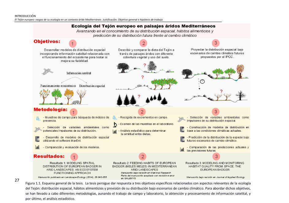
Figura 1.1. Esquena general de la tesis. La tesis persigue dar respuesta a
tres objetivos específicos relacionados con aspectos relevantes de la
ecología del Tejón: distribución espacial, hábitos alimenticios y previsión
de su distribución bajo escenarios de cambio climático. Para abordar
dichos objetivos, se han llevado a cabo diferentes metodologías,
aunando el trabajo de campo y laboratorio, la obtención y
procesamiento de información satelital, y por último, el análisis
estadístico. ................................................................................................. 27
2. ÁREA DE ESTUDIO
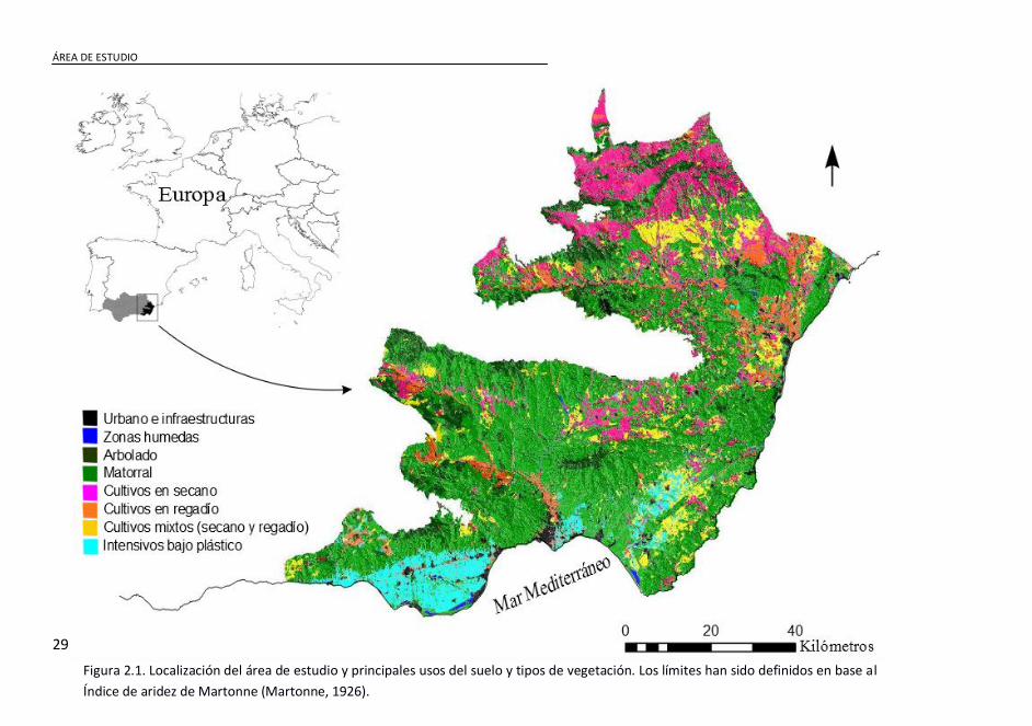
Figura 2.1. Localización del área de estudio y principales usos del suelo y
tipos de vegetación. Los límites han sido definidos en base al Índice de
aridez de Martonne (Martonne, 1926). ....................................................... 29
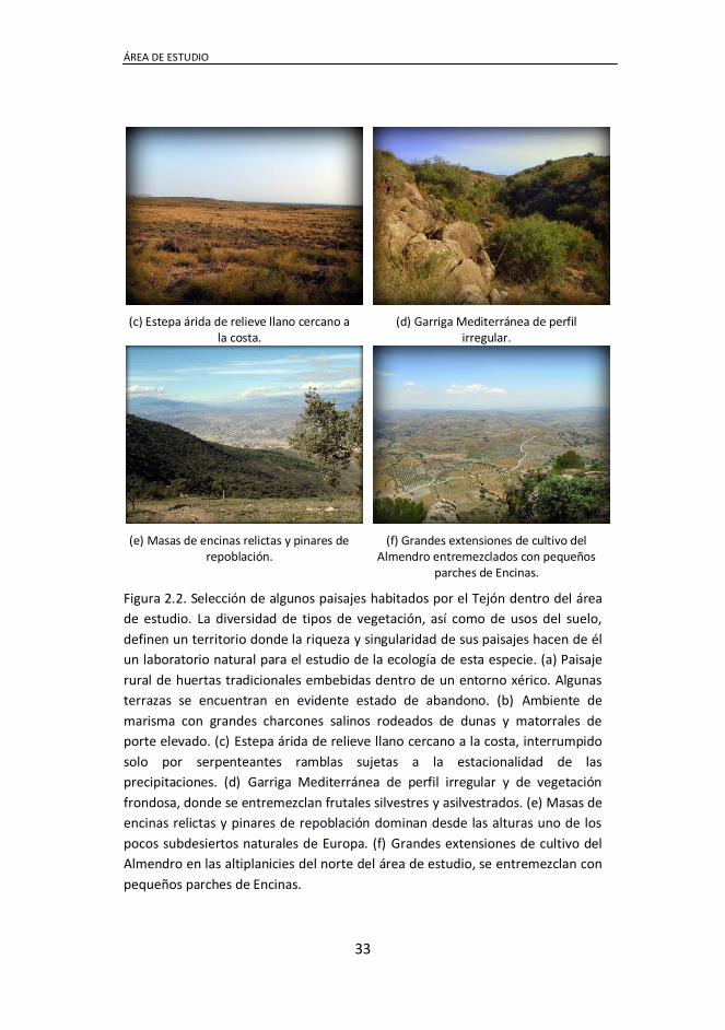
Figura 2.2. Selección de algunos paisajes habitados por el Tejón dentro
del área de estudio. La diversidad de tipos de vegetación, así como de
usos del suelo, definen un territorio donde la riqueza y singularidad de
sus paisajes hacen de él un laboratorio natural para el estudio de la
ecología de esta especie. (a) Paisaje rural de huertas tradicionales
embebidas dentro de un entorno xérico. Algunas terrazas se encuentran
en evidente estado de abandono. (b) Ambiente de marisma con grandes
charcones salinos rodeados de dunas y matorrales de porte elevado. (c)
Estepa árida de relieve llano cercano a la costa, interrumpido solo por
serpenteantes ramblas sujetas a la estacionalidad de las precipitaciones.
(d) Garriga Mediterránea de perfil irregular y de vegetación frondosa,
donde se entremezclan frutales silvestres y asilvestrados. (e) Masas de
encinas relictas y pinares de repoblación dominan desde las alturas uno
de los pocos subdesiertos naturales de Europa. (f) Grandes extensiones
15
de cultivo del Almendro en las altiplanicies del norte del área de estudio,
se entremezclan con pequeños parches de Encinas..................................... 33
3. MATERIAL Y MÉTODOS
Figura 3.1. Esquema gráfico de la metodología empleada en la tesis
doctoral. EVI: Índice de Vegetación Mejorado; MaxEnt: Máxima Entropía;
GLMs: Modelos Lineales Generalizados; GAMs: Modelos Aditivos
Generalizados; NMDS: Escalamiento Multidimensional No Paramétrico;
R: software R .............................................................................................. 35
Figura 3.2. Atributos funcionales derivados del Índice de Vegetación
Mejorado (EVI) y relacionados con el funcionamiento del ecosistema.
Figura modificada de G. Baldi (http://lechusa.unsl.edu.ar) y Alcaraz-
Segura (2005).............................................................................................. 38
4. RESULTADOS
RESULTADO 4.1: MODELING SPATIAL DISTRIBUTION OF EUROPEAN
BADGER IN ARID LANDSCAPES: AN ECOSYSTEM FUNCTIONING
APPROACH
Figure 4.1.1. Study area location. ................................................................ 47
Figure 4.1.2. Jackknife test of variable importance for European badger in
the ALL model with maximum AUCPO. (a) Bars show the AUCPO with each
variable modeled separately. Ratios above the bars show the AUCPO
percentage of the reference value (0.831); (b) Bars show the AUCPO, when
each variable is extracted from the model. The ratios above the bars
show the ratio decreased by the AUCPO with respect to the reference
value (0.831). .............................................................................................. 60

16
RESULTADO 4.2: FEEDING HABITS OF EUROPEAN BADGER (MELES MELES)
IN MEDITERRANEAN ARID LANDSCAPES
Figure 4.2.1. Location of landscapes within the study area in Almería
province, Spain. In each landscape, we identified a zone with latrines
frequently used by European badger (Meles meles). Then, we drew a 3
km-radius buffer zone using the latrines as centroid. .................................. 76
Figure 4.2.2. Estimated relative volume (%) for each main category
considered in the different seasons and landscapes. Whiskers represent
the standard error of the mean values of categories. .................................. 85
Figure 4.2.3. Interaction between landscape and season for earthworm
relative volume (%) in the diet. Whiskers represent the standard error of
the mean values of categories. .................................................................... 86
Figure 4.2.4. Nonparametric multidimensional scaling (NMDS). The axis
NMDS1 and NMDS2, show the range of the distances reached between
seasons in the three landscapes. Seasons are arranged so that the
distances between them are as close to the real differences between the
mean relative volume (%) of fruits, vertebrates and invertebrates
consumed in each landscape. A lower distance between seasons means
greater similarity between them and vice versa. Isoplets are based on the
Shannon´s diversity index. .......................................................................... 88
RESULTADO 4.3: MODELING AND MONITORING HABITAT QUALITY FROM
SPACE: THE EUROPEAN BADGER
Figure 4.3.1. (a) MaxEnt-modeled decrease in habitat suitability of the
European badger in SE arid Spain from current climate conditions (1971-
2000) to two future climate scenarios (IPCC A2 and B1 for 2071-2099).
Habitat suitability maps with mean suitability computed by rows and
columns (cell size 100 x 100 m) in the margins. X and Y axes show UTM
coordinates (Zone 30, Datum ED1950). Cells in grey contain greenhouses,

17
so they were removed before computing the predictions (see
“Environmental variables” subsection). Histograms (Y axis: number of
cells/number total of cells) of the habitat suitability values. (b) Study area
(7051km2) and location of the 179 badger presence records used in this
study. The area only includes arid climate; based on Martonne aridity
index. (c) MaxEnt-modeled maps of significant differences in habitat
suitability between current and predicted climate conditions under the
A2 and B1scenarios for the European badger in SE arid Spain. In pale red,
areas where the variables are expected to significantly decrease (SD >
0.975); in blue, areas where the variables are expected to significantly
increase (SD < 0.025); and in grey, areas where there was no significant
difference. ................................................................................................ 113
Figure 4.3.2. MaxEnt-modeled maps of the limiting factors of habitat
suitability for the European badger in SE arid Spain under current climate
conditions (1971-2000) and two future climate scenarios (IPCC A2 and B1
for 2071-2099). The limiting factor is the environmental variable whose
value at one cell most influences the model suitability prediction. (see
“Environmental variables” subsection for variables abbreviations) ........... 115
Figure 4.3.3. Maps of the significant differences in the EVI descriptors of
ecosystem functioning and in the climate variables between current
climate conditions (1971-2000) and two future climate scenarios (IPCC
A2 and B1 for 2071-2099) in SE Spain. In pale red, areas where the
variables are expected to significantly decrease (SD > 0.975); in blue,
areas where the variables are expected to significantly increase (SD <
0.025); and in grey, areas where there was no significant difference. (see
“Environmental variables” subsection for variables abbreviations) ........... 117

INTRODUCCIÓN El Tejón europeo: rasgos de su ecología en un contexto árido Mediterráneo. Justificación. Objetivo general e hipótesis de trabajo
18
1. INTRODUCCIÓN
(Fotografía: letrina de Tejón en el inferior de la imagen dominando los
rebosantes desiertos del sureste europeo. Paraje Natural del Desierto de
Tabernas, Almería).

INTRODUCCIÓN El Tejón europeo: rasgos de su ecología en un contexto árido Mediterráneo. Justificación. Objetivo general e hipótesis de trabajo
19
1.1 El Tejón europeo: rasgos de su ecología en un
contexto árido Mediterráneo
El Tejón europeo (Meles meles L., 1758) es un carnívoro de mediano
tamaño perteneciente a la familia Mustelidae. Su cuerpo es robusto y
alargado, con cabeza pequeña y cuello muy corto. Posee fuertes patas
acabadas en largas y poderosas uñas que le sirven para excavar. Su
diseño facial es muy característico y consiste en un fondo blanco surcado
por dos bandas negras que cubren la zona de los ojos (Virgós, 2005). La
especie está presente en casi toda Eurasia, aunque su abundancia y/o
presencia no es homogénea a lo largo de su rango de distribución (Virgós
& Casanovas, 1999). Así, en paisajes humanizados del Reino Unido, se
han registrado densidades de más de 40 tejones/km2 (Macdonald &
Newman, 2002) mientras que en algunas zonas del sur de la Península
Ibérica, las densidades no superan 1 tejón/km2 (Revilla et al., 2001a). Esta
variabilidad en su abundancia pone de manifiesto su gran versatilidad
ecológica, pudiendo sobrevivir en una amplia variedad de paisajes,
aunque no con el mismo éxito reproductivo. En Europa centro-
occidental, países escandinavos y Reino Unido, los tejones viven
generalmente en bosques de hoja caduca con alternancia de pastizales
(Kruuk, 1989; Feroe & Montgomery, 1999). En zonas del suroeste de la
Península Ibérica, el matorral mediterráneo representa su hábitat
preferido (Revilla et al., 2000), mientras que en el sureste, donde
aumentan las condiciones de aridez, los tejones seleccionan paisajes
mosaico constituidos por cultivos extensivos mezclados con parches de
vegetación natural (Lara-Romero et al., 2012). Esta capacidad para
adaptarse y sobrevivir en distintos paisajes viene determinada por la
amplitud de estrategias tróficas que es capaz de adoptar. El Tejón es

INTRODUCCIÓN El Tejón europeo: rasgos de su ecología en un contexto árido Mediterráneo. Justificación. Objetivo general e hipótesis de trabajo
20
considerado un especialista en el consumo de lombrices (Lumbricus spp.)
en Gran Bretaña y otras zonas del noroeste de Europa (Kruuk & Parish,
1981). En la región Mediterránea, la disponibilidad de lombrices es
menor debido principalmente a una menor precipitación y a un manejo
del suelo distinto al de otras zonas del norte de Europa (Virgós et al.,
2005a). En estos ambientes, la especie se comporta como un generalista
trófico (Roper, 1994), y consume frutos, insectos y vertebrados en las
zonas más áridas (Piggozi, 1991; Rodríguez & Delibes, 1992; Barea-Azcón
et al., 2010). No obstante, puede mostrar especialización en el consumo
de lombrices en zonas montañosas más húmedas, comportándose por
tanto, como un especialista facultativo bajo circunstancias específicas
(Virgós et al., 2004).
El Tejón europeo ha sido ampliamente estudiado, y sus tendencias
poblacionales y distribución seguidas con interés en el área templada del
continente europeo, especialmente en las Islas Británicas. Gran parte de
este interés se debe a que en dichas zonas la especie representa un
reservorio de Mycobacterium bovis, una micobacteria causante de la
Tuberculosis bovina en el ganado vacuno (Muirhead et al., 1974). Las
investigaciones han mostrado una asociación entre las infecciones de los
rebaños y la presencia de tejones afectados en la misma zona (Muirhead
et al., 1974; Wilesmith, 1983). Por el contrario, en la región
Mediterránea, los estudios sobre la ecología y conservación del Tejón
fueron muy escasos hasta comienzos del siglo XXI, llegando incluso a
catalogarse como “especie insuficientemente conocida” en el Libro Rojo
de los Vertebrados de España (Blanco & González, 1992). En el caso
particular de la Península Ibérica, es a partir del año 2000 cuando
aumenta considerablemente el conocimiento de la especie gracias a los

INTRODUCCIÓN El Tejón europeo: rasgos de su ecología en un contexto árido Mediterráneo. Justificación. Objetivo general e hipótesis de trabajo
21
estudios científicos realizados por diferentes equipos de investigación y a
la labor del Grupo de Carnívoros Terrestres de la SECEM (Sociedad
Española para la Conservación y Estudio de los Mamíferos) (Virgós et al.,
2005b). La información acumulada durante los últimos 20 años ha
permitido su catalogación actual como especie en Riesgo menor (LC)
(Palomo et al., 2007).
En el sur de la Península Ibérica, los trabajos sobre la ecología del Tejón
se han centrado en el Parque Nacional de Doñana y algunas zonas
puntuales en el sureste de Andalucía (Rodríguez & Delibes, 1992; Barea-
Azcón et al., 2010; Lara-Romero et al., 2012). Los paisajes áridos
Mediterráneos, particularmente los situados en el sureste ibérico,
suponen un reto para la supervivencia del Tejón. Estos ambientes
representan el límite de su rango de distribución (Del Cerro et al., 2010),
situándose muy por debajo de la idoneidad de hábitat de los paisajes
centroeuropeos (Lara-Romero et al., 2012). Dicha idoneidad puede
incluso verse disminuida en el futuro, dado que la región Mediterránea
es una de las zonas más susceptibles a sufrir los efectos derivados de
algunos impulsores directos de Cambio Global (ej., cambio climático y
cambios en la cobertura vegetal y de uso del suelo) (Sala et al., 2000;
Giorgi & Lionello, 2008). En el sureste de la Península Ibérica se espera un
incremento considerable de las condiciones de aridez debido a un
aumento de la temperatura y disminución de la precipitación (Giorgi &
Lionello, 2008), pudiendo crear condiciones particularmente difíciles
durante el periodo estival (De Luís et al., 2001). Sin embargo, a pesar de
las consecuencias que los cambios en el clima y en los usos del suelo
pueden suponer para la supervivencia del Tejón (Virgós et al., 2005c), no
existe mucho conocimiento sobre la repercusión que estos impulsores

INTRODUCCIÓN El Tejón europeo: rasgos de su ecología en un contexto árido Mediterráneo. Justificación. Objetivo general e hipótesis de trabajo
22
pueden tener para la especie en ambientes áridos Mediterráneos. Esto
enfatiza la necesidad de avanzar en la comprensión de aspectos clave de
su ecología como son: (1) qué factores ambientales impulsan su
distribución espacial, (2) variabilidad de los hábitos alimenticios de la
especie en un contexto árido Mediterráneo, y (3) cambios potenciales en
su distribución espacial derivados de la proyección a condiciones
climáticas futuras.
Los modelos de distribución espacial tratan de estimar la idoneidad
relativa de hábitat requerida por una especie en un área geográfica
determinada (Warren & Seifert, 2011; Menke et al., 2009). Estas técnicas
representan una herramienta muy útil en la biología de la conservación,
por lo que su uso se está viendo incrementado considerablemente en los
últimos años (Austin, 2007). Actualmente, los modelos de distribución
desarrollados para el Tejón, integran observaciones de presencia de la
especie junto con variables ambientales de tipo topográfico, climático y
de cobertura y uso del suelo, implementados en Sistemas de Información
Geográfica (SIGs) (Virgós & Casanovas, 1999; Jepsen et al., 2005;
Newton-Cross et al., 2007). Estos modelos han mejorado nuestra
comprensión de su distribución y abundancia (Newton-Cross et al.,
2007), reduciendo muchas de las limitaciones asociadas al muestreo de
campo (ej., alto coste económico, limitación en la extensión del área
geográfica estudiada). Sin embargo, la información derivada de
cartografía SIG también posee limitaciones de representatividad
ecológica, tales como, no representar características del paisaje
relevantes para la especie objeto de estudio, o mostrar una resolución
espacial inadecuada a la escala de trabajo seleccionada (Pearce et al.,
2001). Con el fin de avanzar sobre estos problemas, algunos autores

INTRODUCCIÓN El Tejón europeo: rasgos de su ecología en un contexto árido Mediterráneo. Justificación. Objetivo general e hipótesis de trabajo
23
proponen utilizar información satelital para estimar variables que
describan atributos relacionados con el funcionamiento del ecosistema a
través de la producción vegetal (Pettorelli et al., 2005; Cabello et al.,
2012a). Estos atributos describen la variabilidad espacio - temporal de la
producción primaria (Alcaraz-Segura et al., 2013; Requena-Mullor et al.,
2014), por lo que podrían resultar útiles en la modelización de la
distribución espacial del Tejón. Además, gracias a su respuesta rápida
ante los cambios ambientales (Pettorelli et al., 2011), pueden ayudar a
detectar zonas susceptibles de disminuir su calidad de hábitat bajo
condiciones climáticas futuras.
Otro aspecto clave de la ecología del Tejón en paisajes áridos, es su
alimentación. Se ha demostrado que la diversidad de paisajes y de
condiciones ambientales propician distintas estrategias alimenticias en
los tejones, lo que puede condicionar a su vez diferentes organizaciones
sociales, densidades, y afectar a otros aspectos socio-ecológicos (Virgós
et al., 2005a). Por tanto, conocer los hábitos alimenticios de la especie en
paisajes áridos Mediterráneos, es fundamental para comprender de qué
manera pueden variar en respuesta a los principales impulsores de
Cambio Global, y afectar a rasgos importantes de su ecología. Los
estudios sobre la dieta del Tejón en ambientes áridos de la Península
Ibérica son muy escasos. Rodríguez & Delibes (1992) describieron la dieta
únicamente durante la estación de verano en un paisaje con vegetación
xerofítica y cultivos. Barea-Azcón et al. (2010), estudiaron la dieta anual
del Tejón en una zona con clima continental pero en un año
especialmente seco, y un paisaje dominado por Olivos (Olea europea),
pinares (Pinus halepensis) y encinas (Quercus rotundifolia). En este
sentido, no existen estudios que hayan realizado un seguimiento anual

INTRODUCCIÓN El Tejón europeo: rasgos de su ecología en un contexto árido Mediterráneo. Justificación. Objetivo general e hipótesis de trabajo
24
de la dieta en ambientes con aridez constante en el tiempo y analizando
además la influencia de diferentes coberturas vegetales y usos del suelo.
Por último, profundizar en cómo la distribución del Tejón puede variar
ante futuros escenarios climáticos resulta fundamental para entender los
procesos relacionados con la pérdida de su calidad de hábitat. De forma
general, Levinsky et al. (2007) prevén una reducción drástica de la
riqueza potencial de mamíferos en la región Mediterránea, y
particularmente, Maiorano et al. (2014) predicen una disminución de
hasta un 50% en la distribución de las especies de la familia Mustelidae
en la cuenca Mediterránea. Dado que el Tejón es escaso o está ausente
en ambientes áridos Mediterráneos (Virgós et al., 2005c), sería de
esperar que su distribución se viera modificada en respuesta a cambios
ambientales. Estas previsiones ofrecen una excelente oportunidad para
mejorar nuestro conocimiento acerca de los impactos potenciales que el
cambio climático pudiera tener sobre la especie y analizar posibles
respuestas frente a ellos. A su vez, arrojaría información útil para el
desarrollo de planes de conservación, tanto para el Tejón, como para
otros meso carnívoros Mediterráneos.
1.2 Justificación
El Tejón europeo posee una amplia distribución en la Península Ibérica
(Revilla et al., 2002). Sin embargo, a una menor escala, la especie
presenta claras tendencias en sus preferencias de hábitat (Virgós &
Casanovas, 1999; Revilla et al., 2000), y puede llegar a ser localmente
raro o incluso estar ausente, como ocurre en algunas zonas del sureste
árido (Virgós, 1994; Virgós et al., 2005a). El sureste de la Península
Ibérica representa uno de los límites de su distribución, y por tanto, las

INTRODUCCIÓN El Tejón europeo: rasgos de su ecología en un contexto árido Mediterráneo. Justificación. Objetivo general e hipótesis de trabajo
25
condiciones ambientales se encuentran lejos de su óptimo
Centroeuropeo (Virgós & Casanovas, 1999). Por ello, sería razonable
pensar que la supervivencia de la especie en esta región pueda verse
amenazada en un contexto de Cambio Global, por lo que mejorar nuestra
comprensión sobre la ecología de la especie en estos ambientes resulta
determinante. Aunque existe un amplio conocimiento en otras zonas de
su rango de distribución (ej., Europa central e Islas Británicas), en la
región Mediterránea es aún insuficiente, particularmente en ambientes
áridos. A pesar de que en los últimos años se ha avanzado en esta
dirección (Barea-Azcón et al., 2010; Lara-Romero et al., 2012), aún
quedan aspectos importantes por comprender como cuáles son los
factores ambientales que impulsan su distribución espacial, la
variabilidad de sus hábitos alimenticios dentro de un contexto árido o los
patrones futuros de dicha distribución frente a escenarios de cambio
climático.
1.3 Objetivo general e hipótesis de trabajo
El objetivo general de la tesis es avanzar en el conocimiento sobre la
ecología del Tejón europeo en paisajes áridos Mediterráneos (Fig. 1.1).
Para lograr dicho objetivo se proponen tres objetivos específicos:
1. Desarrollar modelos de distribución espacial incorporando
información satelital relacionada con el funcionamiento del
ecosistema, para testar si mejora la fiabilidad de los mismos.
2. Describir y comparar la dieta del Tejón a través de paisajes
áridos con diferente cobertura vegetal y uso del suelo.

INTRODUCCIÓN El Tejón europeo: rasgos de su ecología en un contexto árido Mediterráneo. Justificación. Objetivo general e hipótesis de trabajo
26
3. Proyectar la distribución espacial del Tejón utilizando
escenarios de cambio climático futuros propuestos por el
Intergovernmental Panel on Climate Change (IPCC).
Para ello, se plantean las siguientes hipótesis de trabajo:
1) Dado que los recursos tróficos del tejón están relacionados
directa y/o indirectamente con la producción primaria del
ecosistema, cabría esperar que información derivada de sensores
remotos, relacionada a través de la producción vegetal con el
funcionamiento del ecosistema, resultara útil en la modelización
de la distribución espacial del Tejón.
2) Debido al carácter generalista descrito para el Tejón en
ambientes Mediterráneos (Roper, 1994), el comportamiento
trófico de la especie podría variar entre paisajes áridos con
diferente cobertura vegetal y uso del suelo, y explotar distintos
recursos alimenticios.
3) Los cambios en los patrones de precipitación y temperatura
previstos por los modelos de circulación general de la atmósfera
(IPCC, 2013) podrían reducir hasta en un 50% el rango de
distribución de las especies de la familia Mustelidae en la cuenca
Mediterránea (Maiorano et al., 2014). Por tanto, cabe esperar
una reducción general de la calidad del hábitat para el Tejón en
el sureste árido de la Península Ibérica.
INTRODUCCIÓN El Tejón europeo: rasgos de su ecología en un contexto árido Mediterráneo. Justificación. Objetivo general e hipótesis de trabajo
27
Figura 1.1. Esquena general de la tesis. La tesis persigue dar respuesta a tres objetivos específicos relacionados con aspectos relevantes de la ecología
del Tejón: distribución espacial, hábitos alimenticios y previsión de su distribución bajo escenarios de cambio climático. Para abordar dichos objetivos,
se han llevado a cabo diferentes metodologías, aunando el trabajo de campo y laboratorio, la obtención y procesamiento de información satelital, y
por último, el análisis estadístico.

ÁREA DE ESTUDIO
28
2. ÁREA DE ESTUDIO
La tesis ha sido llevada a cabo en el sureste de la Península Ibérica
(3606’N, 217’E) (Fig. 2.1). Esta región ocupa una posición biogeográfica
singular en el contexto del Mediterráneo occidental. Situada en una zona
de "sombra de lluvias" al abrigo del macizo montañoso de Sierra Nevada,
se encuentra protegida de las borrascas atlánticas que entran por el
oeste, y expuesta a las particularidades climáticas del Mar de Alborán,
con perturbaciones estacionales que dejan intensas lluvias de carácter
torrencial. Así, el rango de precipitación media oscila entre 165-419
mm/año. Dicha personalidad pluviométrica, unida a la rigurosidad
térmica de los veranos mediterráneos y a unas temperaturas suaves el
resto del año (temperatura media de las mínimas: -1.6–15 °C,
temperatura media de las máximas 17-24.5 °C), dibujan uno de los
entornos de aridez más intensos de Europa, con una evapotranspiración
potencial media de 343-1038 mm/año. Junto a todo esto, la región de
estudio ofrece gradientes altitudinales que van desde el nivel del mar
hasta los 1500 m, así como una variedad de litologías que derivan en una
variedad paisajística notable y por tanto, en una oferta de nichos
ecológicos muy diversa.
La región acoge tres pisos termoclimáticos: termo, meso y
supramediterráneo dentro de los sectores biogeográficos almeriense,
alpujarreño-gadorense, nevadense y guadiciano-bacense. Su litología
está caracterizada por la presencia de materiales metamórficos
paleozoicos y paleozoico-triásicos, representados mayoritariamente por
micaesquistos, además de materiales sedimentarios con calizas, margas,
yesos, y arenas terciarias, junto a conglomerados y arcillas cuaternarias.
ÁREA DE ESTUDIO
29 Figura 2.1. Localización del área de estudio y principales usos del suelo y tipos de vegetación. Los límites han sido definidos en base al
Índice de aridez de Martonne (Martonne, 1926).

ÁREA DE ESTUDIO
30
La vegetación más extendida se corresponde con las series termo-
mediterránea semiárida del Arto (Maytenus senegalensis subsp.
europaeus) y termo- y meso-termo-mediterránea del Lentisco,
representadas por Lentiscares con Pistacia lentiscus, Chamaerops humilis
y Rhamnus spp., junto con extensas zonas de matorral de Albaida
(Anthyllis spp.), Esparto (Macrochloa tenacissima) y Tomillos (Thymus
spp.). Puntualmente importantes son los complejos politeselares de
vegetación edafoxerófila sobre yesos con matorrales de pequeño porte.
La vegetación arbórea se asienta en las zonas más elevadas, con
encinares basófilos y silíceos junto a extensas plantaciones de pino (P.
halepensis, P. nigra y P. silvestris). Cabe destacar, por la relevancia
ecológica para el Tejón (Corbacho et al., 2003), las ramblas y cauces
ocupados por geoseries edafohigrófilas donde destacan: Aneas (Typha
spp.), Carrizo (Phragmites autralis), Tarays (Tamarix spp.), Adelfa (Nerium
oleander) y frutales como la Higuera (Ficus carica) y el Algarrobo
(Ceratonia siliqua).
Pero sin duda, uno de los rasgos del área de estudio más destacados y de
mayor trascendencia sobre la ecología del Tejón europeo, son los usos
agrícolas del suelo derivados de la actividad humana (Lara-Romero et al.,
2012). El paisaje rural Mediterráneo ha sido definido como un mosaico
cambiante constituido por cultivos extensivos mezclados con parches de
vegetación natural, favorecedor de la diversidad y abundancia de
carnívoros (Pita et al., 2009). Dichos paisajes mantienen una alta
heterogeneidad paisajística con gran variedad de cultivos, pero
manteniendo a su vez ribazos y linderos. Aunque en retroceso por
abandono, aún se conservan "vegas" asociadas a los cursos de agua,
especialmente en los tramos medios, donde el cultivo de olivos y cítricos

ÁREA DE ESTUDIO
31
son los más destacados. En contraposición, existen extensas áreas de
cultivo intensivo en regadío de olivos, así como de especies herbáceas
(ej., lechuga) y en secano (almendro y cereal), éstos últimos
especialmente importantes hacia el norte. De igual forma, por debajo de
la mitad sur y cercanos al litoral, aparecen tres importantes núcleos de
cultivo hortícola intensivo bajo plástico. El grado de antropización
urbanística, y por tanto, de ocupación humana, es máximo hacia la costa,
disminuyendo en el interior. El éxodo de la población rural desde las
zonas del interior hacia el litoral, especialmente en el sur, representa el
motivo principal de la disminución y deterioro del paisaje rural
tradicional sufrido en las últimas décadas en la región de estudio (Castro
et al., 2011).
Tanto el desarrollo urbanístico como la actividad agrícola intensiva,
ejercen importantes presiones, y por tanto amenazas, sobre la
conservación de los hábitats ocupados por el Tejón, plasmadas por
ejemplo, en la pérdida y fragmentación del hábitat (Virgós et al., 2005c).
En relación a este aspecto, el área de estudio y zonas aledañas, cuentan
con diferentes figuras de protección fruto de las políticas de
conservación del territorio en las últimas décadas. Así, las zonas
montañosas gozan en general de un buen estatus de protección, ej.,
Parque Nacional y Natural de Sierra Nevada, Parque Natural de Sierra
María-Los Vélez y Paraje Natural de Sierra Alhamilla. Los ambientes de
humedal poseen un moderado nivel de protección hacia el sur (ej., Paraje
Natural de Punta Entinas-Sabinar) y casi inexistente en zonas del noreste.
El paisaje estepario, muy extendido a lo largo del área, presenta
diferentes grados de protección. Así, el Parque Natural de Cabo de Gata-
Níjar, Paraje Natural del Desierto de Tabernas y Karst en Yesos de Sorbas,

ÁREA DE ESTUDIO
32
y varios LICs (Lugares de Interés Comunitario) repartidos por el centro y
sur de la región, conforman un gradiente decreciente de conservación de
dicho paisaje. Los ecosistemas esteparios han sido poco valorados
tradicionalmente por el ser humano, sin embargo, son también
explotados por el Tejón aunque en menor proporción. Por último, cabe
destacar la ausencia en la mayoría de los casos, de figuras de protección
que recaigan directamente sobre agroecosistemas tales como las vegas
fluviales tradicionales comentadas antes, o los paisajes cerealistas del
altiplano en la zona norte aledaña al área de estudio. Ambos representan
paisajes humanizados pero de gran valor ecológico, muy importantes
para el Tejón a escala regional (Virgós et al., 2002; Lara-Romero et al.,
2012).
A modo de ejemplo representativo de la diversidad de paisajes presentes
en el área de estudio, la Fig. 2.2 muestra una selección de localidades en
las cuales se ha detectado la presencia de la especie a lo largo de la
realización de la tesis doctoral.
(a) Paisaje rural de huertas tradicionales. (b) Ambiente de marisma.
ÁREA DE ESTUDIO
33
(c) Estepa árida de relieve llano cercano a la costa.
(d) Garriga Mediterránea de perfil irregular.
(e) Masas de encinas relictas y pinares de repoblación.
(f) Grandes extensiones de cultivo del Almendro entremezclados con pequeños
parches de Encinas.
Figura 2.2. Selección de algunos paisajes habitados por el Tejón dentro del área
de estudio. La diversidad de tipos de vegetación, así como de usos del suelo,
definen un territorio donde la riqueza y singularidad de sus paisajes hacen de él
un laboratorio natural para el estudio de la ecología de esta especie. (a) Paisaje
rural de huertas tradicionales embebidas dentro de un entorno xérico. Algunas
terrazas se encuentran en evidente estado de abandono. (b) Ambiente de
marisma con grandes charcones salinos rodeados de dunas y matorrales de
porte elevado. (c) Estepa árida de relieve llano cercano a la costa, interrumpido
solo por serpenteantes ramblas sujetas a la estacionalidad de las
precipitaciones. (d) Garriga Mediterránea de perfil irregular y de vegetación
frondosa, donde se entremezclan frutales silvestres y asilvestrados. (e) Masas de
encinas relictas y pinares de repoblación dominan desde las alturas uno de los
pocos subdesiertos naturales de Europa. (f) Grandes extensiones de cultivo del
Almendro en las altiplanicies del norte del área de estudio, se entremezclan con
pequeños parches de Encinas.

ÁREA DE ESTUDIO
34
De forma particular, y con el fin de testar cada una de las hipótesis
planteadas en la tesis doctoral, se han definido con posterioridad
distintas zonas dentro del área de estudio. Su definición se ha realizado
atendiendo a los requerimientos derivados del planteamiento conceptual
y metodológico de cada hipótesis, y son expuestos detalladamente en el
apartado de resultados.

MATERIAL Y MÉTODOS Trabajo de campo y laboratorio, información satelital - funcionamiento ecosistémico y análisis estadístico
35
3. MATERIAL Y MÉTODOS
La metodología desarrollada en esta memoria de tesis doctoral integra
tres bloques de trabajo principales (Fig. 3.1). BLOQUE I: técnicas de
muestreo en campo y trabajo de laboratorio; BLOQUE II: descarga y
procesamiento de información satelital para la estima de atributos
funcionales del ecosistema empleados como subrogados de la dinámica
espacio - temporal de la producción primaria; y por último, BLOQUE III:
análisis estadístico paramétrico y no paramétrico empleando el software
libre R (R Core Team, 2014) para, a partir de la información obtenida en
los dos bloques anteriores, testar las hipótesis planteadas.
Figura 3.1. Esquema gráfico de la metodología empleada en la tesis doctoral.
EVI: Índice de Vegetación Mejorado; MaxEnt: Máxima Entropía; GLMs: Modelos
Lineales Generalizados; GAMs: Modelos Aditivos Generalizados; NMDS:
Escalamiento Multidimensional No Paramétrico; R: software R.
MATERIAL Y MÉTODOS Trabajo de campo y laboratorio, información satelital - funcionamiento ecosistémico y análisis estadístico
36
3.1 BLOQUE I: Trabajo de campo y laboratorio
El trabajo de campo ha consistido en la búsqueda activa de indicios de
presencia de Tejón y la recolección de excrementos. Existen numerosas
técnicas de campo aplicables al muestreo de la presencia de Tejón (ver
Virgós & Revilla, 2005 para una revisión y resumen). Sin embargo, no
todas son válidas en zonas con baja densidad de la especie como ocurre
en el sureste árido de la Península Ibérica (Lara-Romero et al., 2012). En
este contexto, un método fiable, rápido y barato para cubrir grandes
extensiones, es la búsqueda activa de indicios de presencia (huellas
principalmente) en cuadrículas de igual área y durante un tiempo
determinado (Revilla et al., 2001b). No obstante, dado que la impresión
de huellas es muy dependiente del tipo y estado del sustrato, es
recomendable no limitar la búsqueda únicamente a huellas y ampliarla
también a letrinas y tejoneras (Virgós & Revilla, 2005). La información
levantada en campo, ofrece no solo una serie de localizaciones con
presencia de la especie (coordenadas UTM) imprescindibles para la
modelización de su distribución espacial, sino que posibilita además el
conocimiento de zonas de marcaje con letrinas para la recolecta de
excrementos y su posterior análisis en laboratorio.
El trabajo de laboratorio se ha basado en el análisis visual de
excrementos. Existen diversos protocolos estandarizados para el
reconocimiento y conteo de restos de alimento en heces animales (Kruuk
& Parish, 1981; Pigozzi, 1991). La disgregación de las muestras se realiza
en medio acuoso, para posteriormente, tamizarlas y separar los
componentes. Para el reconocimiento y determinación de los restos de
presas consumidas, se utiliza la lupa binocular, en caso de ítems
macroscópicos (ej., semillas, huesos, restos quitinosos de invertebrados,

MATERIAL Y MÉTODOS Trabajo de campo y laboratorio, información satelital - funcionamiento ecosistémico y análisis estadístico
37
etc.), o el microscopio óptico para la detección de restos más diminutos
como las quetas de las lombrices de tierra.
3.2 BLOQUE II: Información satelital y funcionamiento
ecosistémico
La información espectral emitida por la vegetación y obtenida a partir de
sensores remotos representa un nuevo paradigma para el estudio y
seguimiento de la fauna y su conservación (Pettorelli et al., 2011; Cabello
et al., 2012a). La respuesta espectral de la cobertura vegetal en
longitudes de onda en el rango del rojo e infrarrojo permite estimar
diferentes atributos funcionales sobre grandes extensiones del territorio
(Running et al., 2000; Paruelo et al., 2005), posibilitando a su vez el
estudio del funcionamiento de la vegetación a escala de ecosistema
(Lloyd, 1990). Un ejemplo de ello lo constituye el Índice de Vegetación
Mejorado (EVI), el cual ha sido ampliamente usado como un subrogado
de la Producción Primaria (PP) y su dinámica estacional (Pettorelli et al.,
2005; Alcaraz-Segura et al., 2013) (Fig. 3.2). La ecuación utilizada para su
obtención se indica a continuación:
(1)
donde G es un factor de ganancia; RIRC, RR y RA son respectivamente los
valores de reflectancia bidireccional de la superficie de la tierra para las
bandas del infrarrojo cercano, del rojo y del azul con una corrección de
los efectos de la atmósfera (Absorción de ozono y Rayleigh); C1 y C2 son
los coeficientes de resistencia de aerosoles, que usan la banda azul para
corregir la influencia del aerosol en la banda roja y L es un ajuste del
fondo del dosel que toma en cuenta la transferencia radiante diferencial
del infrarrojo cercano y el rojo a través del dosel. Los coeficientes

MATERIAL Y MÉTODOS Trabajo de campo y laboratorio, información satelital - funcionamiento ecosistémico y análisis estadístico
38
adoptados en el algoritmo del cálculo del EVI son L = 1, C1 = 6, C2 = 7.5 y G
= 2.5. (Fuente: http://modis.gsfc.nasa.gov/data/atbd/atbd_mod13.pdf).
Este índice es un estimador lineal de la fracción de la radiación
fotosintéticamente activa absorbida por la vegetación (fAPAR) (Ruimy et
al., 1994; Huete et al., 2002), el principal control de las ganancias de
carbono (Monteith, 1981), y está siendo cada vez más utilizado en
ecología animal para describir atributos del funcionamiento de los
ecosistemas (Wang et al., 2010; Meynard et al., 2012; Bardsen & Tveraa,
2012; Requena-Mullor et al., 2014).
Figura 3.2. Atributos funcionales derivados del Índice de Vegetación Mejorado
(EVI) y relacionados con el funcionamiento del ecosistema. Figura modificada de
G. Baldi (http://lechusa.unsl.edu.ar) y Alcaraz-Segura (2005).
3.3 BLOQUE III: Análisis estadístico
Con el fin de testar las hipótesis planteadas, la información obtenida en
los bloques I y II ha sido analizada con diversas técnicas estadísticas
utilizando el software libre R.

MATERIAL Y MÉTODOS Trabajo de campo y laboratorio, información satelital - funcionamiento ecosistémico y análisis estadístico
39
3.3.1 Técnicas paramétricas
La modelización de la distribución espacial del Tejón, se ha basado en el
principio de máxima entropía implementado en el software libre MaxEnt
por Phillips et al. (2006). MaxEnt utiliza datos de presencia de la especie
junto a un grupo de pseudo-ausencias escogidas al azar del área de
estudio donde la ausencia y presencia es posible. El objetivo es encontrar
la función de probabilidad que posea la máxima entropía, esto es, la más
cercana a la uniformidad. MaxEnt tiene en cuenta una serie de
restricciones expresadas como funciones simples de las variables
ambientales utilizadas, de tal forma que, el algoritmo aplicado por
MaxEnt obliga a que el promedio de valores obtenidos a partir de las
funciones para cada variable esté próximo a la media empírica conocida
en las localidades con presencia de la especie (Phillips et al., 2004).
Finalmente, el algoritmo otorga un valor de probabilidad de presencia
(asumiendo por defecto que la prevalencia es 0.5) para cada una de las
unidades espaciales en las que haya sido dividida el área de estudio.
Para testar potenciales diferencias entre las estrategias tróficas
desarrolladas por el Tejón en los paisajes estudiados, se realizó un
análisis de varianzas mediante Modelos Lineales Generalizados (GLMs).
Los GLMs son una extensión de los modelos lineales que permiten utilizar
distribuciones de probabilidad no normales para la variable respuesta.
Un GLM consiste en tres componentes:
1.- La distribución de probabilidad de la variable respuesta. Si la variable
respuesta es continua, puede asumirse que su distribución será normal,
con media μ y varianza σ2.
MATERIAL Y MÉTODOS Trabajo de campo y laboratorio, información satelital - funcionamiento ecosistémico y análisis estadístico
40
2.- Componente sistemático. Es una combinación lineal de variables
predictoras continuas y/o categóricas. Cuando estas variables son
únicamente categóricas, el GLM es equivalente al análisis de varianzas
empleado en estadística aplicada (Sokal & Rohlf, 1995; Underwood,
1997).
3.- Función de enlace. Define la relación entre la media de la variable
respuesta y el componente sistemático. Cuando se asume que la relación
entre ambos es lineal, se emplea la función identidad, donde g(μ) = μ.
En los GLMs la estimación de los parámetros se realiza mediante el
método de máxima verosimilitud. El principio en el cual se basa la
estimación por máxima verosimilitud es simple: dada una muestra de
observaciones, el valor estimado para un parámetro es aquél que
maximiza la probabilidad de dichas observaciones.
Los GLMs son considerados modelos paramétricos porque debe
especificarse una distribución de probabilidad para la variable respuesta,
y por tanto, para el término de error del modelo. Así mismo, se
consideran lineales porque la variable respuesta es descrita como una
combinación lineal de variables predictoras. Más información sobre estos
modelos puede encontrase en Agresti (1996) y Myers & Montgomery,
(1997).
3.3.2 Técnicas no paramétricas
Los Modelos Aditivos Generalizados (GAMs) son modificaciones no
paramétricas de los GLMs donde cada variable predictora es incluida en
el modelo como una función no paramétrica de "suavizado" (del inglés
smoothing) (Hastie & Tibshirani, 1990). Estas funciones suelen ser LOESS
smoothing (local regression smoother) o cubic splines (para una
MATERIAL Y MÉTODOS Trabajo de campo y laboratorio, información satelital - funcionamiento ecosistémico y análisis estadístico
41
explicación en detalle ver respectivamente Keele, 2008; Wood, 2006;
entre otros). De forma breve, LOESS smoothing, consiste en un ajuste de
modelos de regresión lineal de forma local a través de pequeñas
"ventanas" de tamaño ajustable a lo largo del eje de abscisas, donde los
puntos dentro de cada ventana son utilizados en un modelo de regresión
para predecir el valor de la variable respuesta correspondiente al valor
medio o a la mediana de la variable predictora dentro de la
correspondiente ventana. En cubic splines, el eje de abscisas es dividido
en varios segmentos, y en cada uno de ellos, una función polinómica de
grado 3 es ajustada.
Los GAMs permiten relaciones no lineales entre la variable respuesta y
las variables predictoras, por lo que resultan muy útiles en situaciones
donde las relaciones lineales no son esperables. Este puede ser el caso de
la relación entre el EVI medio anual y la precipitación media anual (ver
Figura J.1 en Appendix J).
Por último, la búsqueda de similaridad-disimilaridad entre paisajes y
estaciones del año en relación a los alimentos consumidos por el Tejón
requiere de técnicas multivariantes que no asuman normalidad entre las
variables predictoras. El Escalamiento Multidimensional No Paramétrico
(NMDS) es una técnica multivariante de interdependencia que trata de
representar en un espacio geométrico de pocas dimensiones
(normalmente dos) las similaridades existentes entre un conjunto de
objetos (ej., las estaciones del año). De esta manera, una menor distancia
entre los objetos indica mayor semejanza entre las variables predictoras
utilizadas (ej., alimentos consumidos).

RESULTADO 4.1 Modeling spatial distribution of European badger in arid landscapes: an ecosystem functioning approach
42
4. RESULTADOS
RESULTADO 4.1: MODELING SPATIAL DISTRIBUTION
OF EUROPEAN BADGER IN ARID LANDSCAPES: AN
ECOSYSTEM FUNCTIONING APPROACH
Tejón inspeccionando madrigueras de conejo en busca de presas. Escena
capturada con fototrampeo en la Rambla de las Amoladeras. Mayo 2011. Parque
Natural de Cabo de Gata-Níjar.
Basado en:
Juan M. Requena-Mullor, Enrique López, Antonio J. Castro, Javier Cabello,
Emilio Virgós, Emilio González-Miras, Hermelindo Castro. (2014).
Landscape Ecology, 29:843-855.

RESULTADO 4.1 Modeling spatial distribution of European badger in arid landscapes: an ecosystem functioning approach
43
Objetivo 1: “Desarrollar modelos de distribución espacial incorporando
información satelital relacionada con el funcionamiento del ecosistema,
para testar si mejora la fiabilidad de los mismos.”
Hipótesis 1: “Dado que los recursos tróficos del tejón están relacionados
directa y/o indirectamente con la producción primaria, cabría esperar
que la información satelital relacionada con el funcionamiento del
ecosistema a través de la producción vegetal, resultara útil en la
modelización de la distribución espacial del Tejón.”
Tengo mis resultados hace tiempo, pero no sé cómo llegar a ellos.
C. F. Gauss
RESULTADO 4.1 Modeling spatial distribution of European badger in arid landscapes: an ecosystem functioning approach
44
Abstract
Understanding the factors determining the spatial distribution of species
is a major challenge in ecology and conservation. This study tests the use
of ecosystem functioning variables, derived from satellite imagery data,
to explore their potential use in modeling the distribution of the
European badger in Mediterranean arid environments. We found that
the performance of distribution models was enhanced by the inclusion of
variables derived from the Enhanced Vegetation Index (EVI), such as
mean EVI (a proxy for primary production), the coefficient of variation of
mean EVI (an indicator of seasonality), and the standard deviation of
mean EVI (representing spatial heterogeneity of primary production). We
also found that distributions predicted by remote sensing data were
consistent with the ecological preferences of badger in those
environments, which may be explained by the link between EVI-derived
variables and the spatial and temporal variability of food resource
availability. In conclusion, we suggest the incorporation of variables
associated with ecosystem function into species modeling exercises as a
useful tool for improving decision-making related to wildlife conservation
and management.
Keywords: Ecological niche modeling, MaxEnt, remote sensing, EVI, land
use-land cover, Mediterranean ecosystems, Spain, Meles meles

RESULTADO 4.1 Modeling spatial distribution of European badger in arid landscapes: an ecosystem functioning approach
45
4.1.1 Introduction
Understanding the factors determining the spatial distribution of species
is a major challenge in ecology and conservation biology (Brown et al.,
1995). The European badger (Meles meles) is medium-sized carnivore
widely distributed across Europe. In Mediterranean arid landscapes the
species is not abundant or is absent due to extreme aridity (Virgós et al.,
2005). Current spatial distribution models for the European badger use
occurrence data in conjunction with environmental variables derived
from GIS data sources, such as topographic, climatic, and land cover/use
(Virgós & Casanovas, 1999a; Jepsen et al., 2005; Newton-Cross et al.,
2007). These models have improved our understanding of badger
distribution and abundance (Newton-Cross et al., 2007) by reducing
limitations associated with field sampling (e.g., high economic cost and
limited geographic range). However, data derived by GIS cartography
could include limitations of ecological representativeness such as not
representing relevant landscape features for the target species or
inadequate spatial resolution (Pearce et al., 2001).
The use of ecosystem functioning variables could improve spatial
distribution modeling due to their capacity to reflect spatial variability of
landscape features and faster response to environment changes
(Pettorelli et al., 2011). Ecosystem functioning variables can be extracted
from remote sensing imagery, available continuously, both spatially and
temporally. This allows the employment of standardized spectral indexes
for monitoring species on different spatiotemporal scales (Nilsen et al.,
2005) reducing extrapolations. An example of potentially useful
ecosystem functioning variables are the functional attributes derived by
the Enhanced Vegetation Index (EVI). The EVI has been used in mammal

RESULTADO 4.1 Modeling spatial distribution of European badger in arid landscapes: an ecosystem functioning approach
46
ecology by Wang et al. (2010), Meynard et al. (2012), and Bardsen &
Tveraa (2012). The EVI is linearly related to ecosystem carbon gains, and
therefore, to net primary productivity (NPP) (Monteith, 1981), which is
used as a surrogate of ecosystem functioning (Alcaraz et al., 2006;
Cabello et al., 2012a). Thus, measures derived from EVI can describe
ecosystem functional attributes (Pettorelli et al., 2005). These attributes
include the mean annual EVI (i.e., surrogate of primary production)
(Huete et al., 1997; Sims et al., 2006) and the coefficient of variation of
mean annual EVI (i.e., indicator of seasonality) (Alcaraz-Segura et al.,
2013).
The Resource dispersion hypothesis posits that the size of badger
territories is mainly linked to the dispersion of food resources
(Macdonald, 1983; Kruuk, 1989; Macdonald & Carr, 1999). This
hypothesis emphasizes the key role of patchiness of food quality in
determining how large badger territories are. For example, habitat
production tends to drive body condition, ultimately influencing fitness
(Woodroffe, 1995). As a consequence, reproductive success of females is
largely dependent on food conditions, which in badgers are mainly linked
to climate factors mediating food abundance (e.g., production of
habitats) (Woodroffe & Macdonald, 1995). Therefore, badger
demography, abundance and social life is mainly shaped by food
availability and predictability (seasonality), which can be assessed by
ecosystem functional attributes derived of spectral vegetation indices
(e.g., Nilsen et al., 2005; Pettorelli et al., 2005; Pettorelli et al., 2006).
The purpose of this study is to test the use of ecosystem functional
variables derived from EVI (e.g., mean annual EVI, coefficient of variation
of mean annual EVI, and spatial deviation of mean annual EVI) to
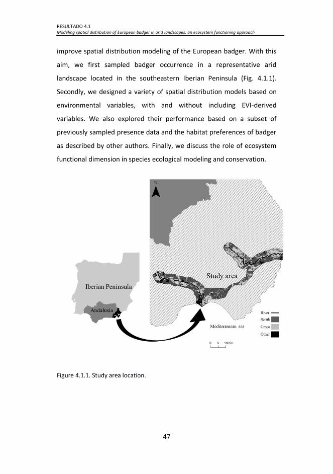
RESULTADO 4.1 Modeling spatial distribution of European badger in arid landscapes: an ecosystem functioning approach
47
improve spatial distribution modeling of the European badger. With this
aim, we first sampled badger occurrence in a representative arid
landscape located in the southeastern Iberian Peninsula (Fig. 4.1.1).
Secondly, we designed a variety of spatial distribution models based on
environmental variables, with and without including EVI-derived
variables. We also explored their performance based on a subset of
previously sampled presence data and the habitat preferences of badger
as described by other authors. Finally, we discuss the role of ecosystem
functional dimension in species ecological modeling and conservation.
Figure 4.1.1. Study area location.

RESULTADO 4.1 Modeling spatial distribution of European badger in arid landscapes: an ecosystem functioning approach
48
4.1.2 Material and methods
4.1.2.1 Study area
We selected a representative area of arid landscapes in the southeastern
Iberian Peninsula based on the Martonne aridity index (Martonne, 1926)
(Fig. 4.1.1), as it is easily calculated and mapped with GIS layers. Inside
this area defined as Arid steppic by the Martonne index (range: 5-15), we
drew a 3.5 km-radius buffer zone on both sides of the two major rivers
basins in the region, and then joined the two buffers (Fig. 4.1.1). In this
form, we ensure inclusion of the potential home range estimated for
European badgers in these environments (i.e., 9 km2) (Lara-Romero et al.,
2012). The study area comprised 835 km2, with a temperature gradient
(range of minimum mean temperatures: 7-12 °C, range of maximum
mean temperatures: 23-28 °C) and an annual precipitation gradient (200-
600 mm/year) associated with a wide altitudinal gradient (0-1400 m).
Evapotranspiration ranges from 93 to 945 mm/year. Another important
feature of the area is the diversity of land cover/use: xerophytic scrubs
represent 48% of the area, where Stipa tenacissima is the most
abundant. Forested habitat is very scarce, corresponding mostly to
scattered pine forests (Pinus halepensis). Crops occupy 27% of the study
area and include fruit orchards (especially abundant near the rivers),
arable crops and greenhouses, in similar proportions.
4.1.2.2 Field survey data
A field survey was conducted from September 2010 to February 2011.
The study area was divided into 5 x 5 km UTM (Universal Transverse
Mercator) plots (out of total 66 plots) to organize the field surveys and
not as the sampling unit. A survey to identify signs of badgers (i.e.,

RESULTADO 4.1 Modeling spatial distribution of European badger in arid landscapes: an ecosystem functioning approach
49
footprints, latrines and setts) was carried out for 6 hours in each plot. To
maximize the detection of the species with the least effort, we selected
places for survey such as paths and catchments for footprints, hills for
latrines and easy to dig sloping areas for setts. These places are known to
be usually used by badgers. The GPS (UTM) coordinates of each sign
were noted with a measurement error of up to 10 m using a GPSmap®
60CSx-Garmin. To avoid spatial autocorrelation of environmental
variables (see below), no signs within 100 m from each other were
considered (see Appendix A).
4.1.2.3 Environmental data
The study area was characterized based on twenty predictor variables
(Table 4.1.1 and Appendix B). Nine of these variables are commonly used
in European badger ecology studies (e.g., Virgós and Casanovas 1999a;
Revilla et al 2000; Jepsen et al., 2005; Macdonald & Newman, 2002;
Rosalino et al., 2008; Lara-Romero et al., 2012), and were comprised by
two climate variables, one topographic variable and six variables related
to habitat structure represented by different land cover/use. The eleven
remaining variables were derived from remote sensing data.
Final resolution of environmental data sets was adjusted to 100 x 100 m
pixel size (i.e., sample unit), to agree with the predominant smallest
spatial resolution of data (Ferrier & Watson, 1997; Elith & Leathwick,
2009). Some variables (i.e., land cover/use variables) were scaled to the
relevant scale for badgers (i.e., their home range).
Topographic and climate variables
Topographic and climate variables were derived from spatial data layers
of the Environmental Information Network of Andalusia

RESULTADO 4.1 Modeling spatial distribution of European badger in arid landscapes: an ecosystem functioning approach
50
(http://www.juntadeandalucia.es/medioambiente/site/web/rediam).
ESRI ArcMapTM 9.3 was used for their handling and processing. The
topographic variable was mean slope, which has been described as a
factor relevant for sett digging (Jepsen et al., 2005). It was estimated
from the digital elevation model of Andalusia with a spatial and elevation
pixel resolution of 20 x 20 m. This layer was resampled to 100 x 100 m.
Climate variables (Virgós & Casanovas, 1999a; Johnson et al., 2002;
Macdonald & Newman, 2002) were mean annual rainfall and the mean
maximum temperature, acquired with a resolution of 100 x 100 m, so no
transformation was made.
Land cover and land use variables
The land cover and land use variables (Virgós & Casanovas, 1999a; Revilla
et al., 2000; Rosalino et al., 2008; Lara-Romero et al., 2012) were derived
from Andalusian Land use/Land cover map (scale 1:25000 from 2007), in
vector format. This layer included the following classes: scattered scrub,
dense scrub, woody crops, arable crops, mixed crops (woody and arable)
and mosaic crops (crops and natural vegetation). The study area was first
divided into 3 x 3 km plots. We estimated the area (km2) of each class
and then we rasterized to 100 x 100 m pixel size. These variables were
scaled because the percent cover is relevant for badgers (Lara-Romero et
al., 2012), instead of using the class of land cover/use as categorical
variable. We considered a 9 km2 area as the probable home range of the
European badger in areas of low habitat suitability (Lara-Romero et al.,
2012).

RESULTADO 4.1 Modeling spatial distribution of European badger in arid landscapes: an ecosystem functioning approach
51
EVI variables
The eleven variables derived from remote sensing data were estimated
based on the MOD13Q1 EVI product, generated from images captured by
the MODIS sensor aboard the NASA’s TERRA satellite
(www.modis.gsfc.nasa.gov) for a period of seven years. These images
have the advantages of its high temporal resolution of 16 days (23
images/year) and spatial resolution appropriate to the scale of the study
(231 x 231 m). The images were subjected to pixel quality filtering, in
which those affected by heavy content of aerosols, clouds, shadows,
snow or water were eliminated. The EVI is the index least affected by
atmospheric conditions and presents fewer saturation problems for high
levels of biomass (Huete et al., 2002).
The mean annual EVI is linearly related to total carbon gain (Running et
al., 2000), and has been used as a surrogate of vegetation production
(Alcaraz-Segura et al., 2013). The standard deviation of mean annual EVI
is an indirect measure of spatial heterogeneity, so that a high standard
deviation may indicate mixed patches, while a low standard deviation is
common in homogeneous landscapes. This variable was estimated by
calculating the standard deviation of mean annual EVI in the 3 x 3 km
plots used to estimate the land cover/use variables. The coefficient of
variation of mean annual EVI is a seasonal carbon gain descriptor (Alcaraz
et al., 2006) that has been used as an indicator of ecosystem seasonality
(Alcaraz-Segura et al., 2013). Furthermore, seasonality, although
described by other variables, has proven decisive in modeling the habitat
of several other species (Boyce, 1978; Ferguson & McLoughlin, 2000;
Wiegand et al., 2008). In addition to these, the EVI autumn mean
(September-November) and EVI spring mean (March-May) were also

RESULTADO 4.1 Modeling spatial distribution of European badger in arid landscapes: an ecosystem functioning approach
52
included as variables, because they represent the two growing seasons in
Mediterranean arid landscapes (Cabello et al., 2012b).
EVI variables were resampled to 100 x 100 m by a bilinear resampling
technique. It determines the new value of a cell based on a weighted
distance average of the four nearest input cell centers. This is likely more
realistic than using nearest-neighbor interpolation method (Phillips et al.,
2006).
EVI of land cover and land uses variables
Five variables were created by calculating mean EVI for each class of land
cover/use referred to above. These variables were also resampled to 100
x 100 m by a bilinear resampling technique.
4.1.2.4 Model building
MaxEnt
We used MaxEnt v. 3.3.3k (Phillips et al., 2006) to model the spatial
distribution of the European badger. The MaxEnt algorithm uses
presence-only data. This is an advantage when working with a very low
density of target species at large scales, as we expected in the study area
based on Lara-Romero et al. (2012), due to the uncertainty in absences.
Although MaxEnt has been criticized on several occasions (see recently
Veloz, 2009; Yackulic et al., 2012), it is widely used for modeling the
spatial distribution of species for various purposes, e.g., testing model
performance against other methods (Elith et al., 2006) and using several
types of variables (Buermann et al., 2008), predicting species richness or
diversity (Graham & Hijmans, 2006), or forecasting distributions to
estimate variations with climate change/land transformation (Yates et

RESULTADO 4.1 Modeling spatial distribution of European badger in arid landscapes: an ecosystem functioning approach
53
al., 2010). Finally, given that 1) the main goal of this study is to test the
performance of models using ecosystem functional variables, and 2)
prediction maps generated by MaxEnt are of interest as assessment
tools, but are not the goal itself, we considered MaxEnt a valid tool for
achieving our objectives.
Models
To test the utility of environmental functional variables in modeling the
spatial distribution of the badger, we combined the twenty variables into
four groups, with and without including ecosystem functional variables
(Table 4.1.1). We defined these four groups because they were the most
ecologically reasonable and of interest for comparison in keeping with
the objectives of this study. These groups of variables, along with the
badger presence data, were input to compute models. We used 10-fold
cross-validation of the occurrence locations. Each partition was made by
randomly selecting 75% of the occurrence locations as training data, and
the remaining 25% as test data. Then, each one of the partitions, along
with each of the four combinations of variables, was run in MaxEnt to
compute the models. We made 10 random partitions rather than a single
one in order to assess the average model behavior, and to allow for
statistical testing of observed differences in performance (Phillips et al.,
2006).
4.1.2.5 Model evaluation
Threshold-independent evaluation
We evaluated the performance of models created from different
combinations of variables using all discriminating thresholds within the
predicted area as suitable or unsuitable for badgers. We used (threshold-

RESULTADO 4.1 Modeling spatial distribution of European badger in arid landscapes: an ecosystem functioning approach
54
independent) receiver operating characteristic (ROC) analysis for this, as
it uses a single measure, the area under the curve (AUC), to show model
performance. With presence-only data, the AUCPO (i.e., AUC estimated
with presence-only data) maximum was less than 1 (Wiley et al., 2003),
so we do not know how close to optimal a given AUCPO was.
Nevertheless, we were able to determine the statistical significance of
the AUCPO and compare the performance of different models (Phillips et
al., 2006). We employed a DeLong test (DeLong et al., 1998) to compare
AUCPO values for each combination of variables. The DeLong test is
designed to nonparametrically compare the difference between two
AUCs from two correlated ROC curves. The Z score is defined as the
difference of AUC divided by its standard error. Under the null hypothesis
(the difference in AUC is zero) Z has a standard normal distribution (Chen
et al., 2013). This test was computed in R (R Development Core Team,
2011).

RESULTADO 4.1 Modeling spatial distribution of European badger in arid landscapes: an ecosystem functioning approach
55
Table 4.1.1. Groups of variables used for constructing models. Group 1: topography and climate, group 2: Land cover and Land uses, group 3: EVI
variables, group 4: EVI of land cover. Each model contained group 1, the ALL model all four groups, LC & LU model groups 1 and 2, the EVI model
groups 1 and 3, and the EVI LC model groups 1 and 4. Thus, three models included the ecosystem functional variables: EVI, EVI LC and ALL, and only
LC & LU model did not include these variables.
Variable Short name Groups of variables
Group 1 Group 2 Group 3 Group 4
Mean slope SLO X Annual Mean Rainfall MRAIN X Mean value of the maximum temperatures MMT X
Area of scattered scrub SSCRUB X
Area of dense scrub SDCRUB X
Area of woody crop SWCROP X
Area of arable crop SACROP X
Area of mixed crop SMICROP X
Area of mosaic crop SMOCROP X
EVI annual mean EVIMEAN X Standard deviation of EVI annual mean EVISTD X Coefficient of variation of EVI annual mean EVICV X EVI autumn mean AEVI X
EVI spring mean SEVI X EVI annual mean of scattered scrub SSCEVI X
EVI annual mean of dense scrub DSCEVI X
EVI annual mean of woody crop WCEVI X
EVI annual mean of arable crop ACEVI X
EVI annual mean of mixed crop MICEVI X
EVI annual mean of mosaic crop MOCEVI X
Group 1: topography and climate, group 2: Land cover and Land use, group 3: EVI variables, group 4: EVI of land cover. Each model
contained group 1, the ALL model all four groups, LC & LU model groups 1 and 2, the EVI model groups 1 and 3, and the EVI LC
model groups 1 and 4. Thus, three models included the ecosystem functional variables: EVI, EVI LC and ALL, and only LC & LU model
did not include these variables.

RESULTADO 4.1 Modeling spatial distribution of European badger in arid landscapes: an ecosystem functioning approach
56
Information criteria
Following Warren & Seifert (2011), we implemented an Akaike
information criterion corrected for small sample size (AICc) (Burnham &
Anderson, 2002) in the MaxEnt models. We standardized raw scores for
each model, so that all scores within the study area added up to 1. Then
we calculated the likelihood of the data in each model by taking the
product of the suitability scores for each pixel showing presence. Both
training and test data were used in calculating likelihood. The number of
parameters was measured by counting all parameters with a nonzero
weight in the .lambda file produced by MaxEnt. All AICcs were computed
using ENMTools software (Warren et al., 2010).
Variable relative importance and response curves
We evaluated the relative importance of the variables using a jackknife
test on the AUCPO found from test data. Thus AUCPO was estimated by 1)
removing the corresponding variable, and then creating a model with the
remaining variables, 2) creating a model using each variable alone, and 3)
using all variables. Furthermore, we plotted the response curves for the
variables which caused the widest variations in the AUCPO. Curves were
estimated by generating a model using only the corresponding variable
and disregarding those remaining (Phillips et al., 2006).
4.1.3 Results
4.1.3.1 Occurrence of European badger
The field survey yielded 94 presence locations, mainly associated with
the two main rivers in the study area (see Appendix C). Landscapes near
the rivers had a larger supply of food resources for the European badger,

RESULTADO 4.1 Modeling spatial distribution of European badger in arid landscapes: an ecosystem functioning approach
57
because crops are abundant there (Fig. 4.1.1). These presence records
are enough for this study since MaxEnt algorithm has been proved to
works well at different sample size (Hernández et al., 2006). 51 of the
records were footprints, 26 latrines, 15 setts and 2 road casualties.
4.1.3.2 Threshold-independent test
In 6 of the 10 partitions, combinations with all variables (ALL) yielded the
models with the highest AUCPO (Table 4.1.2). In 8 of the 10 partitions, the
AUCPO was higher for EVI and EVI LC than for the Land cover & Land uses
models, which were the lowest in most of the partitions.
Table 4.1.2. Comparison of threshold-independent receiver operating
characteristic (ROC) results for European badger using LC & LU, EVI, EVI LC and
ALL models. For each random partition of occurrence records, the maximum
AUCPO is marked in bold, the minimum underlined, and if the observed
difference between the maximum AUCPO and the rest is statistically significant
(under a null hypothesis that true AUCPOs are equal), it is marked with an
asterisk.
Data partition
LC & LU
EVI EVI LC
ALL
AUCPO AUCPO AUCPO AUCPO
1 0.722 0.669 0.725 0.722 2 0.63 0.701 0.634 0.674 3 0.644* 0.705 0.745 0.658 4 0.753* 0.756* 0.761 0.816 5 0.625* 0.785 0.69 0.69* 6 0.742* 0.793* 0.746* 0.808 7 0.734 0.726 0.707 0.741 8 0.673* 0.711 0.682 0.735 9 0.772 0.788 0.753 0.831 10 0.718* 0.758* 0.77 0.82
Average 0.701 0.739 0.721 0.749 Standard deviation
0.053
0.042 0.042
0.065
Maximum 0.772 0.793 0.770 0.831 Minimum 0.625 0.669 0.634 0.658
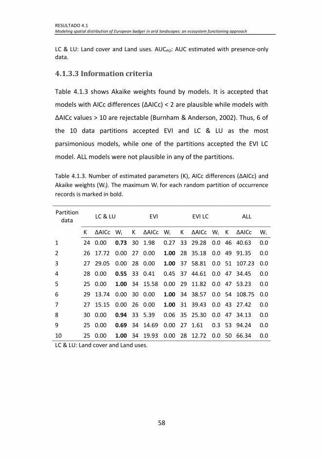
RESULTADO 4.1 Modeling spatial distribution of European badger in arid landscapes: an ecosystem functioning approach
58
LC & LU: Land cover and Land uses. AUCPO: AUC estimated with presence-only data.
4.1.3.3 Information criteria
Table 4.1.3 shows Akaike weights found by models. It is accepted that
models with AICc differences (∆AICc) < 2 are plausible while models with
∆AICc values > 10 are rejectable (Burnham & Anderson, 2002). Thus, 6 of
the 10 data partitions accepted EVI and LC & LU as the most
parsimonious models, while one of the partitions accepted the EVI LC
model. ALL models were not plausible in any of the partitions.
Table 4.1.3. Number of estimated parameters (K), AICc differences (∆AICc) and
Akaike weights (Wi). The maximum Wi for each random partition of occurrence
records is marked in bold.
Partition data
LC & LU EVI EVI LC ALL
K ΔAICc Wi K ∆AICc Wi K ∆AICc Wi K ∆AICc Wi
1 24 0.00 0.73 30 1.98 0.27 33 29.28 0.0 46 40.63 0.0
2 26 17.72 0.00 27 0.00 1.00 28 35.18 0.0 49 91.35 0.0
3 27 29.05 0.00 28 0.00 1.00 37 58.81 0.0 51 107.23 0.0
4 28 0.00 0.55 33 0.41 0.45 37 44.61 0.0 47 34.45 0.0
5 25 0.00 1.00 34 15.58 0.00 29 11.82 0.0 47 53.23 0.0
6 29 13.74 0.00 30 0.00 1.00 34 38.57 0.0 54 108.75 0.0
7 27 15.15 0.00 26 0.00 1.00 31 39.43 0.0 43 27.42 0.0
8 30 0.00 0.94 33 5.39 0.06 35 25.30 0.0 47 34.13 0.0
9 25 0.00 0.69 34 14.69 0.00 27 1.61 0.3 53 94.24 0.0
10 25 0.00 1.00 34 19.93 0.00 28 12.72 0.0 50 66.34 0.0
LC & LU: Land cover and Land uses.

RESULTADO 4.1 Modeling spatial distribution of European badger in arid landscapes: an ecosystem functioning approach
59
4.1.3.4 Relevant variables and their effects
We only analyzed the relative importance of variables from the ALL
model, with the maximum AUCPO value. Area of mosaic crop (SMOCROP)
caused a 2% reduction in AUCPO (Fig. 4.1.2b). Therefore, this variable,
along with others that caused a reduction of over 1% (Area of scattered
scrub (SSCRUB), EVI of mosaic crop (MOCEVI), mean maximum
temperature (MMT) and coefficient of variation of mean EVI (EVICV)),
provided the most useful information not present in the other variables.
We considered reductions about 2% and 1% as relevant, because these
percentages were above the third quartile (0.84%) of reduction values
percentage. EVIMEAN alone had the highest AUCPO (87.4% AUCPO with all
variables) (Fig. 4.1.2a) and therefore, this variable provided the most
useful information by itself. Apart from this, others like EVI spring, EVI
autumn, EVI scattered scrub and standard deviation of mean EVI, were
over 79%.

RESULTADO 4.1 Modeling spatial distribution of European badger in arid landscapes: an ecosystem functioning approach
60
Figure 4.1.2. Jackknife test of variable importance for European badger in the
ALL model with maximum AUCPO. (a) Bars show the AUCPO with each variable
modeled separately. Ratios above the bars show the AUCPO percentage of the
reference value (0.831); (b) Bars show the AUCPO, when each variable is
extracted from the model. The ratios above the bars show the ratio decreased
by the AUCPO with respect to the reference value (0.831).
Variables such as scattered scrub area, mean maximum temperature,
standard deviation of mean EVI and EVI of scattered scrub exerted a
nonlinear effect on European badger habitat suitability, as predicted by
MaxEnt (Appendix D). On the contrary, mosaic crop area and mean
annual EVI, exerted a positive linear effect, while EVI crop mosaic and
coefficient of variation of mean EVI had a negative linear effect.

RESULTADO 4.1 Modeling spatial distribution of European badger in arid landscapes: an ecosystem functioning approach
61
4.1.4 Discussion
4.1.4.1 Did the EVI-derived variables improve ecological
niche modeling of the European badger in arid landscapes?
EVI variables provided useful information that improved the ecological
niche modeling of European badger in arid Mediterranean landscapes.
Based on the AUCPO and AICc criteria, models built with EVI variables,
performed well in predicting the spatial distribution, while models
without them were inferior (based on AUCPO). We suggest that the
variables included in the EVI models underlie the spatiotemporal
dynamic of badger food resources by describing vegetation production
(EVIMEAN), seasonality (EVICV) and spatial heterogeneity (EVISTD). Thus,
areas with high EVI mean and EVI spatial heterogeneity represented
more suitable habitats for the European badger, while they rejected
areas with high EVI seasonality.
Our study showed that despite the fact that rainfall (expressed here as
mean annual rainfall, MRAIN) is considered the main driver of vegetation
growth in Mediterranean environments (Nemani et al., 2003), it did not
prove to be as good a predictor as the mean EVI (as proxy of primary
production) for European badger distribution. The higher performance of
EVI mean can be explained by the findings of Cabello et al. (2012b), in
which production derived from EVI in drylands reflects the variation of
the water use efficiency and its availability due to the features of
vegetation and lithology. In addition, EVI mean also reflected the NPP for
irrigated crops, which do not depend directly on rainfall (33% of crops in
the study area are irrigated).

RESULTADO 4.1 Modeling spatial distribution of European badger in arid landscapes: an ecosystem functioning approach
62
Additionally, more seasonal environments in the study area (i.e., with
high EVICV values) represented zones with low habitat quality for
European badger. Johnson et al. (2002) suggested that badger densities
across Europe are associated with seasonal constraints, or some other
constraint(s) that covary with seasonality. EVI models predicted as
suitable, landscapes with little annual variation in EVI values,
corresponding with sites where the availability of food may be assured
even in summer, the season experiencing the most extreme shortages in
food. Similarly, Virgós & Casanovas (1999a) showed that a decrease in
summer rainfall reduces badger occurrence in Mediterranean mountains.
We also found that badgers selected areas with high EVI spatial
heterogeneity. Pita et al. (2009) described the Mediterranean rural
landscape as a shifting mosaic that benefits diversity and presence of
species as the European badger. The different types of traditional crops,
along with patches of semi-natural vegetation, especially scrub and/or
forest, yield a wide variety of food resources. We argue that the EVISTD
variable might detect these mosaic landscapes. However, although this
variable contributed positively to European badger habitat suitability, its
effect was nonlinear, suggesting that badgers would not need such
heterogeneity to survive in certain landscapes.
Both EVICV and EVISTD might depict variability of resources availability.
EVICV represents temporal variability in the availability of resources
because it is the dispersion of mean EVI throughout the year. In this
sense, if EVI in summer and winter are significantly different, the annual
temporal variability of EVI will be large. On the other hand, EVISTD
represents spatial variability because it is the standard deviation of mean

RESULTADO 4.1 Modeling spatial distribution of European badger in arid landscapes: an ecosystem functioning approach
63
EVI into the potential territories of badgers. In consequence, high values
indicate that a landscape will be more heterogeneous.
4.1.4.2 Was the predicted spatial distribution across arid
lands consistent with the ecological preferences of the
European badger?
The distribution predicted by the EVI models was coherent with the
habitat preferences described for the European badger (see Appendix E
for further details of predicted distributions by models). Our results
reveal that badger´s presence in the study area was mainly associated
with sites near rivers where there were several different types of crops
and patches of natural vegetation. According to Lara-Romero et al.
(2012), in Mediterranean drylands the European badger prefers mosaic
landscapes consisting of fruit orchards and natural vegetation, which
provide shelter and food resources. In these environments, the diet is
diversified, with consumption of fruit increasing in some seasons (Barea-
Azcón et al., 2010). Fruits, insects and vertebrates have also been
described as relevant food resources for European badger in
Mediterranean environments (Rodríguez & Delibes, 1992; Revilla &
Palomares, 2002). Likewise, other authors have related the occurrence or
abundance of these items with satellite-derived vegetation indices, such
as EVI or Normalized Difference Vegetation Index (NDVI) (see Willems et
al., 2009; Lafage et al., 2013; Tapia et al., 2013).
EVI and EVI for Land cover models discriminated better between suitable
(i.e., mosaic landscapes with crops) and unsuitable areas (homogeneous
patches of dense xerophytic scrubs) than the LC & LU models (see Table
4.1.2 and Appendix E). EVI variables provided information for
discriminating between two patches with the same type of land use and

RESULTADO 4.1 Modeling spatial distribution of European badger in arid landscapes: an ecosystem functioning approach
64
cover, but with different primary production, seasonality and spatial
heterogeneity. The EVI for Land cover models exhibited an intermediate
performance (Table 4.1.2). These models also used variables related to
primary production. However, such variables were averaged based on
the spatial classification derived by GIS cartography. These maps may not
represent relevant landscape features for the target species or
inadequate spatial resolution (Pearce et al., 2001).
Sites with high EVIMEAN and SMOCROP (area of mosaic crops) values
represented the most suitable habitats for the European badger.
However, the variable EVI mean of mosaic crops (MOCEVI) showed a
negative effect on badger presence, which could be explained by the fact
that 1- mosaic crop variable, in turn, encompasses different types of
crops, and 2- badger presence records with high EVI values, are
associated with non-irrigated almond crop, which would not favor
badger presence in those areas. This suggests that in particular
landscapes, the type of land use would be more decisive for badger than
its associated production.
Removal of variables such as SWCROP (area of woody crop) and AEVI (EVI
autumn), did increase performance, meaning that such variables reduced
the generality of the model. This is, models made with these variables
appear to be less transferable to other geographic areas or to projected
future distributions by applying future conditions (Phillips, 2006).
Regarding the potential bias of the selected study area on results, we
consider that the study area contained enough variability to ensure that
its effect was minimized. Probably, a larger buffer would provide similar
results because the area between both rivers has not crops. In

RESULTADO 4.1 Modeling spatial distribution of European badger in arid landscapes: an ecosystem functioning approach
65
Mediterranean arid landscapes, the major landscape variability is
generally associated with areas near rivers (Corbacho et al., 2003) and
along altitudinal gradients, just what we defined with our study area.
4.1.4.3 Ecosystem functional dimension in species
ecological modeling and conservation
The incorporation of remotely sensed characterization of the ecosystem
functional dimension in management and monitoring of species and
populations is gaining attention in conservation biology (Cabello et al.,
2012a). Ecosystem functional dimension provides proxies showing
biodiversity patterns and new tools and criteria that can assist in
designing conservation planning and actions. Some examples are shown
by Bardsen & Tveraa (2012), who used vegetation production estimated
by EVI to advance knowledge of the reproductive biology of reindeer
(Rangifer tarandus) in Norway; Oindo (2002), who predicted mammal
species richness and abundance using multi-temporal NDVI data; or
Wiegand et al. (2008), who studied the relationship between brown bear
(Ursus arctos) habitat quality and the seasonal course of NDVI as a proxy
for ecosystem functioning in the northern Iberian Peninsula.
Ecological modeling of the European badger in the Iberian Peninsula has
to date been addressed mainly using landscape structural variables
estimated from visual field observation (transect scale) (Virgós &
Casanovas, 1999b) and by GIS information (regional scale) (Rosalino et
al., 2004). Even though these variables that reflect landscape structure
are essential to modeling the species distribution (Rosalino et al., 2008),
they do not reflect the role of ecosystem functioning indicators or their
bidirectional relationship with the conservation of biodiversity and
ecosystem processes (Cabello et al., 2012a). However, Pettorelli et al.
RESULTADO 4.1 Modeling spatial distribution of European badger in arid landscapes: an ecosystem functioning approach
66
(2005) and García-Rangel & Pettorelli (2013) point out some constrains of
remote sensing data to wildlife studies such as select the most suitable
processing to eliminate noise in the data, insufficient temporal resolution
to precisely date phenological phenomena, and economic disadvantages
due to many satellites still produce data that are not free.
Our study is the first to show that incorporation of ecosystem functional
variables (EVI-derived) improves the prediction of spatial distribution
modeling of the European badger in arid landscapes, considered
especially sensitive to Global Change (Lavorel et al., 1998). In this sense,
Pettorelli et al. (2005) suggested that satellite-derived indexes, such NDVI
or EVI, could be used to predict the ecological effects of environmental
change on ecosystems functioning and animal population dynamics and
distributions, due to their correlation with vegetation biomass and
relationship with climate variables.
Finally, we found that EVI variables represented relevant ecological
parameters for the description of the distribution of the European
badger as they can indicate 1) a high NPP associated with orchards or
fruit crops, very important for its survival in Mediterranean arid
landscapes (Rodríguez & Delibes, 1992; Lara-Romero et al., 2012), 2)
seasonality in the primary production, which can be seen as a surrogate
of habitat quality (Johnson et al., 2002), and 3) spatially heterogeneous
landscapes which provide different food resources (Pita et al., 2009).
However, these variables should be tested in other areas of its
distribution range. Models including EVI variables perform better (based
on AUCPO) than models not including these variables. Additionally,
continuous availability, both spatially and temporally, of remote sensing

RESULTADO 4.1 Modeling spatial distribution of European badger in arid landscapes: an ecosystem functioning approach
67
data can improve the accuracy of monitoring and modeling wildlife for
conservation purposes in arid ecosystems throughout the world.

RESULTADO 4.2 Feeding habits of European badger (Meles meles) in Mediterranean arid landscapes
68
RESULTADO 4.2: FEEDING HABITS OF EUROPEAN
BADGER (Meles meles) IN MEDITERRANEAN ARID
LANDSCAPES
Tejón en busca de alimento en la quietud de la noche entre la densidad de la
vegetación de ribera. Escena capturada con fototrampeo en la Rambla de los
Molinos. Abril 2013. Paraje Natural del Desierto de Tabernas.
Basado en:
J. M. Requena-Mullor, E. López, A. J. Castro, E. Virgós, H. Castro. Hábitos
alimenticios del Tejón europeo en un paisaje árido Mediterráneo.
Galemys, aceptado con revisión menor.
J. M. Requena-Mullor, E. López, A. J. Castro, E. Virgós, H. Castro.
Landscape influence in feeding habits of European badger (Meles meles)
in arid Spain. Mammal Research, en revisión.

RESULTADO 4.2 Feeding habits of European badger (Meles meles) in Mediterranean arid landscapes
69
Objetivo 2: “Describir y comparar la dieta del Tejón a través de paisajes
áridos con diferente cobertura vegetal y uso del suelo.”
Hipótesis 2: “Debido al carácter generalista descrito para el Tejón en
ambientes Mediterráneos (Roper, 1994), el comportamiento trófico de la
especie podría variar entre paisajes áridos con diferente cobertura
vegetal y uso del suelo, y explotar en cada caso distintos recursos
alimenticios.”
Somos lo que comemos.
Ludwig Feuerbach.

RESULTADO 4.2 Feeding habits of European badger (Meles meles) in Mediterranean arid landscapes
70
Abstract
This study evaluates the influence of landscape on feeding behavior of
European badger (Meles meles) in southern Iberian Peninsula. We
particularly explore whether different vegetation types and land uses
affect its feeding habits across three arid landscapes; maquia, xeric
shrubland, and forestry. Although diet of badger has been described as
frugivory in Mediterranean environments, with cultivated and wild fruits
as key items (e.g., olives or figs), its feeding strategy may vary in response
to the composition of landscape consuming different key items in an arid
Mediterranean context. Based on 252 scats monthly collected from June
2011 to May 2012, we found that diet significantly varied among
landscapes studied: insects, carob, and small mammals were the key
items in the maquia, figs and oranges in the xeric shrubland, and
earthworms and insects in the forestry. This shows that within an arid
context, badger adapt its feeding behavior to particular landscape
conditions, and specifically, the diet of badgers shift from an animal-
based to another where cultivated fruits reaches the high importance.
Our results support the key role of human activities in shaping badger
behavior and diet and illuminating the contrasting dietary differences of
badger living on more pristine habitats versus those inhabiting human-
made habitats. Based on the proved effect of precipitation and land
management practices on items here identified, we also discuss
implications of Global Change drivers in badgers feeding habits for the
arid Mediterranean region.
Keywords: Meles meles, European badger, mustelids, diet, frugivory,
Iberian Peninsula, drylands, land use-land cover

RESULTADO 4.2 Feeding habits of European badger (Meles meles) in Mediterranean arid landscapes
71
4.2.1 Introduction
Feeding habits of the European badger Meles meles Linnaeus, 1758 have
been extensively studied and are one of its best-known ecological
features (Goszcynski et al., 2000; Virgós et al., 2005a). Their diet is very
diverse throughout their distribution range, with a wide assortment of
trophic strategies (Melis et al., 2002). The European badger is considered
a specialist forager for earthworms in Britain and others areas of
northwest Europe (Kruuk & Parish, 1981; Kruuk, 1989; but see Roper,
1994). In the Mediterranean region, earthworm availability is lower than
in north Europe due to a low precipitation and different landscape
composition (Virgós et al., 2004). In these environments, the species is a
trophic generalist (Roper et al., 1994) consuming fruits, insects, and
vertebrates (Piggozi, 1991; Rodríguez & Delibes, 1992; Barea-Azcón et al.,
2010). However, badgers can also specialize in earthworm consumption
in rainy mountainous Mediterranean areas, so it can be considered as a
facultative specialist at local scale, taking the most profitable resource
depending on supply and availability (Martín et al., 1995; Virgós et al.,
2004).
Despite the discussion about the feeding specialization of badgers, it has
been suggested an important effect of consumption of earthworms as
compared to other trophic resources on life-history traits of the species
such as population density and reproductive success (da Silva et al.,
1993; Woodroffe & Macdonald, 1993; Virgós et al., 2005a). However,
badgers can survive at low densities in extreme arid landscapes (Lara-
Romero et al., 2012; Requena-Mullor et al., 2014), where earthworms
are absent or very scarce. Despite the interest of these regions to a wide
interpretation of feeding strategies of badgers, only two studies dealing

RESULTADO 4.2 Feeding habits of European badger (Meles meles) in Mediterranean arid landscapes
72
with badger diet in arid environments (Rodríguez & Delibes, 1992; Barea-
Azcón et al., 2010). Rodríguez & Delibes (1992) described the diet only
during summer in a landscape with xerophitic vegetation and crops.
Barea-Azcón et al. (2010) analyzed the annual diet in a region with
continental climate (14 °C/year and 620 mm/year) but during an
especially dry year (250 mm), and in a landscape dominated by olive tree
plantations (Olea europea), dense pine forest reforestations (Pinus
halepensis) and some holm oak patches (Quercus rotundifolia) and both
studies emphasized the importance of cultivated fruits and rabbits
(Oryctolagus cuniculus) in the diet of badgers living at these
environments.
Fruits are largely consumed for badgers in some regions, Rosalino &
Santos-Reis (2009) detected an increase in fruit consumption along a
west to east Mediterranean gradient in a diverse guild of frugivory
mammals including the European badger. These authors argued that fruit
consumption depends on several factors such as fruit characteristics
(e.g., pulp content), availability of wild and cultivated fruits, and
abundance of other food resources (see also Herrera, 1989), which vary
throughout the Mediterranean basin. In fact, some authors have
highlighted cultivated fruits as a key food resource for badgers in
Mediterranean arid environments (Pigozzi, 1991; Rodríguez & Delibes,
1992; Barea-Azcón et al., 2010) which encourage the importance of the
orchards as a key habitat for the species in these environments (Lara-
Romero et al., 2012; Requena-Mullor et al., 2014). Thus, in arid habitats,
cultivated fruits could replace earthworms as the key food in badger life-
history traits, allowing increase its abundance and performance.

RESULTADO 4.2 Feeding habits of European badger (Meles meles) in Mediterranean arid landscapes
73
Feeding strategies of badgers are very flexible and current tactics can be
modified if environmental conditions change. The Mediterranean region
is especially vulnerable to Global Change drivers (Sala et al., 2000; Giorgi
& Lionello, 2008). Aridity is expected to increase in the Iberian Peninsula,
especially in arid zones (Giorgi & Lionello, 2008) due to increasing
temperatures and decreasing rainfall, particularly during summer months
(De Luis et al., 2001). Additionally, agricultural lands represent more than
half of the Mediterranean region by area (Olesen & Bindi, 2002). The
reform of the Common Agricultural Policy (PAC) for 2014-2020 outlines
steps to promote crop diversification, establish and maintain permanent
pastures, and leave some land fallow to restore natural ecological
processes (Martínez & Palacios, 2012). These measures would benefit
the conservation of badger populations in Mediterranean environments
(Virgós et al., 2005b). Nevertheless, aging of the rural population and
young peoples’ exodus to the cities, is leading to widespread land
abandonment in last decades (Castro et al., 2011). This demographic
change is causing a deterioration of the rural Mediterranean landscape
which is very important for the conservation of some species that
depend on agricultural areas (Zamora et al., 2007; Pita et al., 2009). This
is true for badgers, which are very linked to traditional human activities
and agricultural practices, especially in arid environments (Kruuk, 1989;
Virgos et al., 2005b; Lara-Romero et al., 2012). Consequently, in the next
future two main changes can modify Mediterranean regions, first most
areas of the Mediterranean can be transformed to arid habitat; second,
most agricultural areas will be abandoned. Under these new scenarios,
food resources for badgers can change dramatically, and this can affect
other life-history traits such as population density, social organization or
population growth (Macdonald & Newman, 2002; Macdonald et al.,

RESULTADO 4.2 Feeding habits of European badger (Meles meles) in Mediterranean arid landscapes
74
2010). Therefore, the diet of badgers in arid regions of the
Mediterranean can offer an opportunity to forecast what resources can
be essentials for badgers in the new scenario of increasing aridity for
most of the Mediterranean region, and elucidate how changes in
agricultural practices can impact on badger diet and then other
important traits of the species.
This study uses three landscapes (maquia, xeric shrubland, forestry) in
environments of southern Iberia Peninsula which represents the extreme
ecological and geographical range of the species to explore whether
different vegetation types and land uses affect the feeding behavior of
badger. Based on previous findings regarding the effect of precipitation
and land management practices on food resources for badgers, potential
implications of Global Change drivers in badgers feeding habits are
discussed for arid Mediterranean areas.
4.2.2 Materials and methods
4.2.2.1 Localization and description of landscapes
This study was conducted in the southeastern Iberian Peninsula (36°06’N,
2°17’E) (Fig. 4.2.1). This region is the most arid in Europe (Armas et al.,
2011), represents some of the most extreme arid conditions inhabited by
badgers, and contains a wide variety of mixed arid environments with
Mediterranean rural landscapes. The aridity of target landscapes was
characterized based on the Martonne aridity index (Martonne, 1926) (Ia),
considering arid climate a Ia between 5 and 15 (Requena-Mullor et al.,
2014).
On a local scale, diet composition of the European badger depends
primarily on the management and soil use by humans (Kruuk, 1989;

RESULTADO 4.2 Feeding habits of European badger (Meles meles) in Mediterranean arid landscapes
75
Fischer et al., 2005). Therefore, to compare the diet among landscapes,
we selected three landscapes with different land cover and use (maquia,
xeric shrubland and forestry). In each landscape, first we identified a zone
with latrines frequently used by the species. Then, we drew a 3 km-
radius buffer zone using the latrines as the centroid (Fig. 4.2.1). This
method ensures the inclusion of the potential home range size estimated
for European badgers living at these poor environments (i.e., 9 km2)
(Lara-Romero et al., 2012). Finally, we characterized the type of land
cover and use within the buffers based on GIS cartography from
Andalusia Land use/Land cover map (scale 1:25.000, 2007).

RESULTADO 4.2 Feeding habits of European badger (Meles meles) in Mediterranean arid landscapes
76
Figure 4.2.1. Location of landscapes within the study area in Almería province,
Spain. In each landscape, we identified a zone with latrines frequently used by
European badger (Meles meles). Then, we drew a 3 km-radius buffer zone using
the latrines as centroid.
Landscape 1: Maquia (37°08’N, 1°55’E)
Maquia has the lowest altitude (102 m) and an Ia of 11.72 (0.004). The
mean annual rainfall is 340 mm/year and mean annual temperature is

RESULTADO 4.2 Feeding habits of European badger (Meles meles) in Mediterranean arid landscapes
77
19°C. The area is mainly dominated by non-forested natural vegetation
(65% of the total area) including dense shrubland (e.g., Macrochola
tenacissima, Pistacia lentiscus) and sparse shrubland (Rhamnus lycioides,
Anthyllis cytisoides). Agricultural uses comprise the 22% of the area,
where homogeneous herbaceous crops (i.e., without natural vegetation)
are predominant, with irrigated and rainfed crops in similar proportions.
It is important to highlight the abundance of wild vegetation with fleshy
fruits (e.g., Ceratonia siliqua, Ficus carica, Chamaerops humilis, Vitis sp.,
O. europea var. silvestris) in the watercourses.
Landscape 2: Xeric shrubland (36°58’N, 2°29’E)
Xeric shrubland is located at 228 m altitude, and has an Ia of 6.98
(0.012). The mean annual rainfall is 200 mm/year and the mean annual
temperature is 18 °C. 70% of the area is covered by sparse xeric
shrubland (M. tenacissima, Salsola genistoides, Anthyllis terniflora).
Crops occupy only the 12% of the landscape, where the 44% of them are
woody irrigated crops (e.g., Citrus sp.) and the rest are greenhouses. The
remaining 18% of the area is occupied by minority uses.
Landscape 3: Forestry (37°06’N, 2°46’E)
Forestry is located at 1320 m altitude, and has an Ia of 12.54 (0.028).
Mean annual rainfall is 310 mm/year and mean annual temperature is
12°C. Natural vegetation covers the 84% of the area, with forestry (e.g.,
Pinus spp.) and shrublands (e.g., Genista spp., Adenocarpus decorticans)
in similar proportions. Agricultural uses represent the 16% of the total
area, in which mosaics of natural vegetation with rainfed crops (O.
europea and Prunus dulcis) are predominant.

RESULTADO 4.2 Feeding habits of European badger (Meles meles) in Mediterranean arid landscapes
78
4.2.2.2 Diet analysis
The analysis of the diet consisted in collecting scats in badger latrines and
examining composition in the laboratory. Faeces were collected once a
month from the latrines across the three target landscapes. Sampling
was conducted from June 2011 to May 2012. In each visit, we recorded
the number of latrines and scats contained. Prior to the collection period,
all scats were removed from latrines at the end of May 2011. Faeces
were classified based on their water content, shape and colour. If this
was impossible, the entire latrine content was taken as a single faeces
(Pigozzi, 1991). Washing and sieving was carried out according to the
Kruuk & Parish (1981) protocol. For each scat, the total number of items
were counted or extrapolated from the remains, following the Kruuk &
Parish (1981) and Pigozzi (1991) methods. Items were gathered in three
broad categories: fruits, vertebrates, invertebrates. Nevertheless, in
order to identify what food resources were dominant within each
landscape, we carried out a finer grouping, classifying each remainder to
the lowest taxonomic level in each case (i.e., species). The food remains
were compared with reference collections to ensure a correct taxonomic
determination. Lastly, data collected was grouped by annual seasons, i.e.,
summer (June, July, August), autumn (September, October, November),
winter (December, January, February), spring (March, April, May). For all
categories (both in the wide and fine classification), we estimated the
frequency of occurrence FO (%) and the relative volume RV (%), the latter
was assessed visually based on the Kruuk & Parish (1981) method. In
addition, we calculated the Shannon´s diversity index for each landscape
and season (Shannon, 1948):
- ∑ lo i (1)

RESULTADO 4.2 Feeding habits of European badger (Meles meles) in Mediterranean arid landscapes
79
where Pi= proportion of each food category. The diversity is minimum
when H = 0 and it is maximum when H = log n (n = number of categories).
We considered three wide categories, so H maximum = 0.47.
4.2.2.3 Data analyses
Landscape type and seasonal differences in the relative volume of wide
categories (i.e., fruits, vertebrates and invertebrates) were analyzed by a
two-way ANOVA with the relative volume of each category as a response
variable and the landscape type and season as fixed factors (Virgós et al.,
2004). When the effects of landscape or season were significant, we
employed a Duncan´s test to reveal which landscapes or seasons showed
large differences in relative volume for each item considered. All
residuals were checked for normality (Shapiro-Wilk Normality test)
(Shapiro & Wilk 1965), and homogeneity of variances (Bartlett test)
(Snedecor & Cochran, 1989). In general, the residuals showed no-
normality and heterocedasticity, so we resampled the data by
bootstrapping (10000 replicates) for estimate the F´s distribution and
recalculated the critical value for signification (i.e., 0.05) (Appendix F).
Due to the importance of earthworms for badgers in others areas of its
distribution (Kruuk, 1989; Virgós et al., 2004), we also analyzed
separately the consumption of this item so that our data can be
compared to previous studies.
Correlations between diet diversity (measured by the Shannon index)
and the relative volume of wide categories, between diet diversity and
main consumed fine categories, and among all wide categories, were
analyzed using the Spearman´s rho statistic (Best & Roberts, 1975).
RESULTADO 4.2 Feeding habits of European badger (Meles meles) in Mediterranean arid landscapes
80
Finally, we used a nonparametric multidimensional scaling (NMDS) to
explore similarities in the diet based on both spatial (landscapes) and
temporal (seasonal) variations. With this aim, we arranged the seasons
for each landscape in a Cartesian axis based on the grouping
consumption of fruits, vertebrates and invertebrates (in RV). Regarding
this, a shorter distance between seasons means greater similarity and
vice versa. We used the Bray-Curtis distance (djk) to compute the NMDS.
∑ – ∑ ii (2)
where x is the RV (%) of food category i (i.e., fruits, vertebrates,
invertebrates) in the j and k seasons. To check the goodness of NMDS we
measured the concordance in the rank order of the observed inter-
season distances and those predicted from the similarities. One measure
of fit is the Kruskal´s stress (Kruskal, 1964). Clarke (1993) provided some
guidelines for stress values, so stress values greater than 0.3 indicate the
achieved configuration is no better than random.
All statistical analyses were carried out using R software version 2.14.2 (R
Development Core Team, 2012)
4.2.3 Results
4.2.3.1 Diet composition
A total of 252 faeces were collected, 54 in maquia, 140 in xeric
shrubland, and 58 in forestry (Table 4.2.1). In maquia, fruits were
consumed throughout the year (annual FO = 81%), although the mean
relative volume was greatly reduced in summer (VR = 29.3% ±4.73 SE).
Carobs were the most frequent fruit in excrements (annual FO = 46.29%)
(see Table G.1 in Appendix G). Grapes (47.5% ±12.5 SE) (summer), carobs
(82% ±8.98 SE and 96.4% ±2.82 SE) (autumn and winter) and oranges

RESULTADO 4.2 Feeding habits of European badger (Meles meles) in Mediterranean arid landscapes
81
(63% ±27.5 SE) (spring) were the fruits with the highest mean relative
volume. Vertebrates were more frequent in spring (FO = 72.7%) (Table
4.2.1), with small-mammals (e.g., rodentia) as key prey and obtaining a
relevant mean volume (RV = 70% ±17.75 SE spring and RV = 82.5% ±8.63
SE winter) (Table G.1). Invertebrates were very frequent in summer (FO =
100%) (Table 4.2.1) (mainly Coleoptera) but in a low mean volume
(25.3% ±5.63 SE) (Table G.1).
Table 4.2.1. Mean relative volume (%) and frequency of occurrence (in
parentheses, %) values for the different wide categories considered in each
landscape and season. We reported values of frequency of occurrence for
comparative purposes with other studies using these categories.
Landscape and prey item Summer Autumn Winter Spring
Maquia
Fruits 29.3 (100) 51.2 (100) 68.0 (72.0) 42.5 (72.7)
Vertebrates 20.3 (16.7) 45.8 (16.7) 76.5 (40.0) 64.1 (72.7)
Invertebrates 15.0 (100) 8.5 (58.3) 34.8 (24.0) 21.1 (36.4)
N 6 12 25 11
Xeric shrubland
Fruits 61.8 (96.2) 88.6 (100) 75.2 (95.5) 74.7 (92.7)
Vertebrates 73.8 (15.4) 20.0 (13.3) 39.5 (22.7) 23.3 (21.8)
Invertebrates 6.8 (42.3) 6.0 (40.0) 18.7 (54.5) 30.3 (70.9)
N 26 15 44 55
Forestry
Fruits 54.6 (41.7) 66.1 (70.0) 68.5 (40.0) 50.1 (9.5)
Vertebrates 30.0 (8.3) 27.6 (30.0) 61.3 (26.7) 53.4 (57.1)
Invertebrates 34.2 (100) 40.0 (80.0) 39.5 (86.7) 35.8 (81.0)
N 12 10 15 21

RESULTADO 4.2 Feeding habits of European badger (Meles meles) in Mediterranean arid landscapes
82
In xeric shrubland, fruits appear to be the key food resource for badger
based on both the frequency of occurrence (annual FO = 95%) and
relative volume (mean annual RV = 73.41% ±2.49 SE). Two types of fruits
were mainly consumed, figs (FO = 73% and 93.3%; mean RV = 78.4%
±6.27 SE and 94% ±2.91 SE) (from summer to autumn) and oranges (FO =
84% and 67.2%; mean RV = 80% ±4.52 SE and 83.6% ±4.42 SE) (from
winter to spring) (Table G.2). Vertebrates had low relevance throughout
the year, appearing only with a considerable volume in summer (mean
RV = 73.8% ±18.18 SE) (Table 4.2.1), with anura (mean VR= 100%) and
rabbits (VR= 87.5% ±2.5 SE) being the predominant taxonomic groups
(Table G.2). Invertebrates were more frequent in spring (FO = 70.9%) and
winter (FO = 54.5%) (Table 4.2.1), although their volume was not
important in any season (mean annual RV = 17.62% ±2 SE). Orthoptera
was the most frequent along the year (annual FO = 34%) (Table G.2).
In forestry there was a high consumption of invertebrates throughout the
year (annual FO = 86%), although with a low relative volume (mean
annual RV = 36% ±3 SE). Scorpions (FO = 50%; mean RV = 35.8% ±5.78 SE)
(summer), Hymenoptera (FO = 60%; mean RV = 54% ±11.57 SE)
(autumn), earthworms (FO = 53.3%; mean RV = 81.8% ±4.99 SE) (winter),
and caterpillars (FO = 66.6%; mean RV = 44.1% ±8.35 SE) (spring) were
the most relevant invertebrates (Table G.3). Fruits were consumed
mainly in autumn (FO = 70%) (Table 4.2.1), with figs (mean RV = 60%
±5.77 SE), wild blackberries (mean RV = 90% ±10 SE) and almonds (mean
RV = 50% ±) (pericarp fleshly) most abundant (Table G.3). The relative
volume of fruits was considerable throughout the year (mean annual RV
= 62% ±6.64 SE). Vertebrates were consumed more frequently in spring
(FO = 57.1%) (Table 4.2.1). Spring and winter were the seasons with the

RESULTADO 4.2 Feeding habits of European badger (Meles meles) in Mediterranean arid landscapes
83
highest volume of vertebrates in the faeces (mean RV = 53.4% ±11.08 SE
and mean RV = 61.3% ±12.31 SE respectively), mainly due to reptiles and
rabbits (Table G.3).
4.2.3.2 Effects of landscape and season on diet
Consumption of fruits showed statistically significant difference for
landscape and season when the two factors were separately considered,
however, the interaction between both factors was not significant (Table
4.2.2). Relative volume was higher in xeric shrubland than in maquia
(Duncan´s test, p < 0.01) (see Fig. 4.2.2). Moreover, fruit consumption
was higher in winter than in summer (Duncan´s test, p < 0.01) (Fig. 4.2.2).
Table 4.2.2. Results of the two-way ANOVA with season and landscape type as
fixed factors and the relative volume of the wide categories as the response
variable. No effect varied its signification by applying the bootstrap resampling
(see Table F.1 Appendix F).
Relative volume Effect df F p
Fruits Season 3 4.04 <0.01
Landscape 2 13.3 <0.001
Season x Landscape 6 1.22 0.29
Vertebrates Season 3 2.07 0.11
Landscape 2 5.56 <0.01
Season x Landscape 6 1.36 0.24
Invertebrates Season 3 2.85 <0.05
Landscape 2 11.61 <0.001
Season x Landscape 6 1.96 0.07
We also observe significant differences in the consumption of
vertebrates between landscapes, but not between seasons (Table 4.2.2).
RESULTADO 4.2 Feeding habits of European badger (Meles meles) in Mediterranean arid landscapes
84
Vertebrates showed significantly higher relative volume in maquia than
in xeric shrubland (Duncan´s test, p < 0.01).
For invertebrate consumption, we observed differences among
landscape and season even though the interaction was marginally not
significant (Table 4.2.2). More invertebrates were consumed by badgers
in forestry than those in maquia and xeric shrubland (Duncan´s test, p <
0.01). Invertebrates were higher consumed in spring than in autumn
(Duncan´s test, p < 0.05).
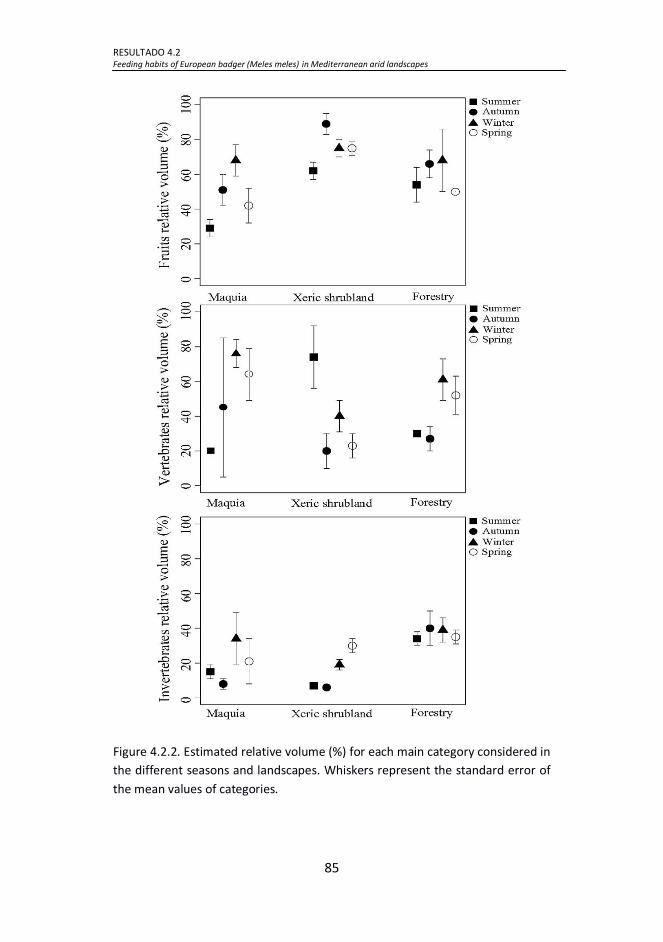
RESULTADO 4.2 Feeding habits of European badger (Meles meles) in Mediterranean arid landscapes
85
Figure 4.2.2. Estimated relative volume (%) for each main category considered in
the different seasons and landscapes. Whiskers represent the standard error of
the mean values of categories.

RESULTADO 4.2 Feeding habits of European badger (Meles meles) in Mediterranean arid landscapes
86
4.2.3.3 Earthworm consumption
Earthworms were consumed in the three landscapes but always with a
low frequency of occurrence (mean annual FO = 3.7%, 2.8% and 17.2%
for maquia, xeric shrubland and forestry respectively) (Tables G.1, G.2
and G.3). However, a high relative volume was found (mean annual RV =
90% ±10 SE, 50% ±12.24 SE and 77.7% ±4.82 SE for maquia, xeric
shrubland and forestry).
For the relative volume, there was only difference between seasons
(ANOVA, F = 59.2, p < 0.0001) and it was higher in winter than in spring
(Duncan´s test, p < 0.0001) (Fig. 4.2.3).
Figure 4.2.3. Interaction between landscape and season for earthworm relative
volume (%) in the diet. Whiskers represent the standard error of the mean
values of categories.

RESULTADO 4.2 Feeding habits of European badger (Meles meles) in Mediterranean arid landscapes
87
4.2.3.4 Diet diversity and food consumption
Diet diversity was similar in the three landscapes, but the more diverse
annual diet was obtained in maquia (H = 0.39), followed by forestry (H =
0.37) and xeric shrubland (H = 0.30). Diet diversity was positively
correlated with fruit and vertebrate consumption (rho = 0.44, p = <0.001,
n = 36; rho = 0.58, p < 0.001, n = 36). Conversely, the diversity was
negatively, but not significantly, correlated with the invertebrate
consumption (rho = -0.17, p = 0.30, n = 36). Food resources with a high
consumption (e.g., carobs, figs, oranges, coleopteran and earthworms,
see Tables G.1, G.2 and G.3) showed a no significant correlation with the
diet diversity, except rodentia which showed positive correlation (rho =
0.41, p < 0.05, n = 36). Between wide categories, relative volume of fruits
and invertebrates showed negative correlation (rho = -0.41, p < 0.05, n =
36), indicating higher consumption of fruits in landscapes or seasons
where invertebrates are not very important in the diet of badgers. Fruits
with vertebrates and vertebrates with invertebrates, showed a low non
significant correlation (rho = -0.03, p = 0.84, n = 36; rho = -0.10, p = 0.53,
n = 36).
4.2.3.5 Nonparametric multidimensional scaling
The spatial configuration reached by the NMDS (Fig. 4.2.4) was better
than random (Kruskal´s stress < 0.2). By seasons, the summer in the
maquia (mean djk = 0.37) and the autumn in the xeric shrubland (mean djk
= 0.31) had the greatest distance (Fig. 4.2.4 and Appendix H).
The diet in the maquia had the greatest distance between seasons (mean
djk = 0.34), while in the xeric shrubland the distances were intermediate
(mean djk = 0.26), and in the forestry, the seasons were the closest (mean

RESULTADO 4.2 Feeding habits of European badger (Meles meles) in Mediterranean arid landscapes
88
djk = 0.15) (Appendix H). The summer in the maquia and the autumn in
the xeric shrubland showed the lowest Shannon´s diversity index (0.26
and 0.27 respectively) (Fig. 4.2.4).
Figure 4.2.4. Nonparametric multidimensional scaling (NMDS). The axis NMDS1
and NMDS2, show the range of the distances reached between seasons in the
three landscapes. Seasons are arranged so that the distances between them are
as close to the real differences between the mean relative volume (%) of fruits,
vertebrates and invertebrates consumed in each landscape. A lower distance

RESULTADO 4.2 Feeding habits of European badger (Meles meles) in Mediterranean arid landscapes
89
between seasons means greater similarity between them and vice versa.
Isoplets are based on the Shannon´s diversity index.
4.2.4 Discussion
4.2.4.1 Spatial and temporal variation of badger diet
Despite of the common arid environmental features across all locations,
badger diet varied significantly across the three landscapes. One or two
dominants food resources in each of the cases studies were identified.
This supports Virgós et al. (2004), in other Mediterranean areas where
feeding behaviour of badgers can vary among close locations but with
different habitat type, rainfall regimen or human land use.
We found that in maquia, badgers were mainly frugivores although
vertebrates were also important in winter and spring. This feeding
strategy has been also described in other Mediterranean areas (Piggozi,
1991; Rosalino et al., 2004). Carobs were the most consumed fruit
throughout the year. This is the first time that this food resource is
described in this type of landscape. Carobs were available and abundant
along the year (personal observation), highlighting the generalist-
opportunist character of the European badger (Pigozzi, 1991). The fruit
consumption was however lower than in xeric shrubland, besides this,
the fruits consumed were mainly wild, so the direct dependence of
badgers for orchards would be less decisive. Small-mammals were the
second most important item, probably providing the necessary proteins
in a vegetarian diet (Ciampalini & Lovari, 1985).
In xeric shrubland, fruits, especially cultivated, were the most important
food resource. Oranges from winter to spring and figs from summer to
autumn as the most consumed items. While figs have been described in

RESULTADO 4.2 Feeding habits of European badger (Meles meles) in Mediterranean arid landscapes
90
dry Mediterranean landscapes as an usual food resource for badgers
(Barea-Azcón et al., 2010), this is the first time that oranges are described
across these environments. This landscape is the most arid of the cases
studies; therefore, the importance of orchards for the survival of badgers
in these environments is reinforced (Lara-Romero et al., 2012).
In forestry, badger diet mainly consisted in insects when frequency of
occurrence was considered, but fruits prevailed again when relative
volume was taken into account. A large consumption of insects supports
findings by Virgós et al. (2004) in some of the habitats sampled in the
mountain areas of central Spain. However, the relevance of fruits also in
this habitat highlights the key importance of this food resource for
badger in all the arid landscapes.
When badgers preferentially consume the same type of food resource
along the year, such as fruits in xeric shrubland or invertebrates in
forestry, the diet similarity between seasons is higher. On the other
hand, the highest distances between seasons (e.g., summer vs. winter in
maquia, summer in xeric shrubland vs. summer in maquia) were mainly
due to the differences in the vertebrates and invertebrates consumption.
In Mediterranean arid landscapes, the availability of earthworms is
scarce (Virgós et al., 2005a). Our results show that badgers consumed
this item across maquia and xeric shrubland, supporting results obtained
by Barea-Azcón et al. (2010), for other Mediterranean area. In forestry,
the consumption of earthworms was even larger than in the other
landscapes. This increase may be due to a greater availability of
earthworms in mid-mountain areas because of the altitude effect, which
causes that rainfall is larger (Virgós et al., 2005a). However, the

RESULTADO 4.2 Feeding habits of European badger (Meles meles) in Mediterranean arid landscapes
91
consumption of earthworms was not uniform across the year, appearing
only in winter and spring, because of this prey item is mainly available in
the rainy and mild conditions of spring and autumn-winter (Edwards &
Lofty, 1977; Kruuk & Parish, 1981). All these results combined reinforce
the usefulness of this trophic resource for badgers when available, and
its large importance even in the extreme arid conditions of the south
edge of its distribution range, contradicting the original ideas about the
unimportance of earthworms in most of the southern badger range
(Ciampalini & Lovari, 1985; Pigozzi, 1991; Roper, 1994; Martín et al.,
1995; but see Virgós et al., 2004).
Olives were not relevant in any of the three landscapes. This disagrees
with findings in other Mediterranean areas (Kruuk & de Kock, 1981;
Rosalino et al., 2004; Barea-Azcón et al., 2010). This may be due to their
low availability in the sampled localities (personal observation), as
expected of a generalist (or facultative specialist) species such as
European badger (Pigozzi, 1991). Badgers shifted their preferences for
different fruits when availability changes.
Our results showed that the diet diversity did not decrease with the
consumption of specific items. This supports the generalist character of
badger in the arid Mediterranean environments described by Rodríguez
& Delibes (1992) and Barea-Azcón et al. (2010). Despite the large
importance of fruits, this cannot be viewed as of similar importance of
earthworms or rabbits in other areas, where diversity is strongly
associated to the consumption of these resources (Kruuk, 1989; Martín
et al., 1995). On the other hand, fruits and invertebrates showed a
negative correlation. An explanation for this could be badgers replace the
shortage of fruits per invertebrates (mainly insects which are predictable

RESULTADO 4.2 Feeding habits of European badger (Meles meles) in Mediterranean arid landscapes
92
and abundant). This supports similar strategy of badgers from the central
Spain mountains when earthworms are scarce (Virgós et al., 2004).
Our results reinforce the feeding behavior described for the European
badger in Mediterranean landscapes by Rodríguez & Delibes (1992) and
Barea-Azcón et al. (2010). We also found that two food resources (i.e.,
oranges and carob trees) have a high presence in the diet, being
described for first time as key food resource in badger survival across
Mediterranean arid landscapes. These items have a clumped distribution,
showing a high seasonal abundance and a high energetic value (Agencia
Andaluza del Agua, 2010). The same features have been cited for other
key resources of the species (Kruuk, 1989; Martín et al., 2005; Rosalino et
al., 2005).
4.2.4.2 Potential implications of climatic change and land
use change on feeding habits
Climate change and land use change have been described as two of the
main direct drivers of Global Change in Mediterranean environments
(Vitousek, 1994; Giorgi & Lionello, 2008). On one hand, it has been
proved that the abundance of European badger is related with climatic
characteristics (Virgós & Casanovas, 1999) and their seasonality (Johnson
et al., 2002). Many of the items consumed by badgers across the three
landscapes depend directly (e.g., carobs, figs, blackberries, fan palm
fruits, earthworms) or indirectly (e.g., insects, small-mammals, rabbits)
on precipitation. Theoretical models about species coexistence predict
that a larger temporal variation of resources reduces probability of
specialization in feeding habits (Wilson and Yoshimura 1994). Regarding
this, badgers would have a facultative specialist behaviour in more
variable environments (Virgós et al., 2004), modifying their feeding

RESULTADO 4.2 Feeding habits of European badger (Meles meles) in Mediterranean arid landscapes
93
strategy and/or the choice of food, in order to maximize the intake in
accordance with their availability (Pigozzi, 1991). Accordingly, the species
would prefer landscapes with a high spatial-temporal predictability in
food resources (Mellgren & Roper, 1986; Kruuk, 1989). These landscapes
could be associated with orchards presence, representing a predictable,
clumped and profitable habitat to provide food for badgers. This has
been recently described by Requena-Mullor et al. (2014), showing that
the presence of agricultural humanized landscapes increases the
opportunity of use different food resources over time and space.
Traditional agricultural practices provide badgers with other food
resources such as figs, loquats, apples, and apricots that also indirectly
depend on irrigation. In addition, because of lower use of pesticides,
traditional agricultural practices also offer a great diversity and
abundance of arthropods (Bengtsson et al., 2005). In the Mediterranean
region, the species selects mosaic landscapes consisting of fruit crops and
orchards, mixed with patches of natural vegetation that provide food and
shelter (Lara-Romero et al., 2012). We found that in xeric shrubland,
badger showed a large preference for oranges, which directly depends
on the irrigation (Agencia Andaluza del Agua, 2010) and for figs, which
depends more directly on the precipitation. Therefore, a reduction of
these food resources by crop abandonment and less precipitation can
affect regional occurrence and abundance, including local extinction
where habitats can be extremely arid.
On the other hand, land cover and use changes influence the feeding
habits of European badger by modifying its feeding strategy and/or the
choice of preys (Kruuk, 1989). On a local scale, the composition of badger
diet depends on the land management and use (Fischer et al., 2005),
RESULTADO 4.2 Feeding habits of European badger (Meles meles) in Mediterranean arid landscapes
94
particularly in agricultural areas (Rosalino et al., 2004; Barea-Azcón et al.,
2010). Kruuk & Parish (1985) described how the feeding of badger varied
with changes in agricultural production in north Scotland. These authors
found that earthworm’s availability decreased during eight years and
badgers offset this reduction eating cereals in the later months. Despite
this, as a consequence they found a body weight reduction in males (i.e.,
14%) and females (17%). This finding suggests that due to extreme
conditions and low badger abundance in Mediterranean arid
environments, a reduction of key food resources may strongly affect
badger fitness (Virgós et al., 2005b).
In conclusion, food resources consumed by badgers depend on both
precipitation and land use-land cover. Therefore, variations predicted on
these factors under future climate change and land use scenarios (IPCC,
2013) may affect badger feeding habits across Mediterranean arid
environments, and be probably translated to changes in regional
distribution, abundance and other life-history traits.

RESULTADO 4.3 Modeling and monitoring habitat quality from space: the European badger
95
RESULTADO 4.3: MODELING AND MONITORING
HABITAT QUALITY FROM SPACE: THE EUROPEAN
BADGER
Tejón aseándose y desparasitándose en las cercanías de su tejonera. Escena
captada con fototrampeo en el paraje Venta de los Yesos. Marzo 2013. Tabernas.
Basado en:
Juan M. Requena-Mullor, Enrique López, Antonio J. Castro, Domingo
Alcaraz-Segura, Hermelindo Castro, Andrés Reyes, Javier Cabello.
Modeling and monitoring habitat quality from space: the European
badger. Journal of Applied Ecology, en revisión.
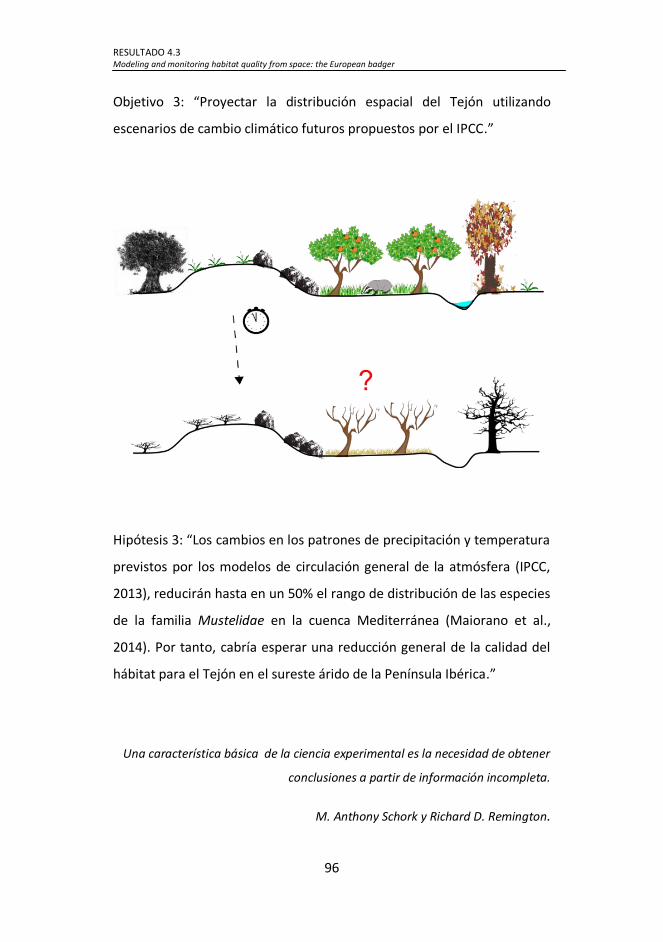
RESULTADO 4.3 Modeling and monitoring habitat quality from space: the European badger
96
Objetivo 3: “Proyectar la distribución espacial del Tejón utilizando
escenarios de cambio climático futuros propuestos por el IPCC.”
Hipótesis 3: “Los cambios en los patrones de precipitación y temperatura
previstos por los modelos de circulación general de la atmósfera (IPCC,
2013), reducirán hasta en un 50% el rango de distribución de las especies
de la familia Mustelidae en la cuenca Mediterránea (Maiorano et al.,
2014). Por tanto, cabría esperar una reducción general de la calidad del
hábitat para el Tejón en el sureste árido de la Península Ibérica.”
Una característica básica de la ciencia experimental es la necesidad de obtener
conclusiones a partir de información incompleta.
M. Anthony Schork y Richard D. Remington.

RESULTADO 4.3 Modeling and monitoring habitat quality from space: the European badger
97
Abstract
1. As climate change is expected to have a significant impact on species
distributions, there is an urgent need to enhance the efficiency of
biodiversity monitoring programs and provide managers with valuable
information to guide and adapt their actions.
2. For the European badger, a species not abundant and at risk of local
extinction due to climate change in the arid environments of
southeastern Spain, we identify which areas are prone to loss or gain of
habitat suitability as a result of climate change. Using MaxEnt, we
designed spatial distribution models for the badger using presence-only
data and climate and EVI-derived variables, and forecast the badger
potential spatial distribution for the 2071- 2099 period based on the IPCC
scenarios.
3. Including remotely sensed descriptors of the temporal dynamics and
spatial patterns of ecosystem functioning into spatial distribution
models, results suggest that high suitability areas for European badgers
may decrease in response to future climate scenarios. Primary
production and ecosystem functional heterogeneity seem to be these
main drivers of change.
4. Synthesis and applications. The incorporation of ecosystem functional
attributes derived from remote sensing in the modeling of future
forecast may contribute to the improvement of the detection of
ecological responses. Because conservation resources are limited, the
monitoring efforts for biodiversity should focus on areas which are more
likely to experience local extinctions or occurrence shifts and on the
involved environmental drivers of change. We suggest that our approach

RESULTADO 4.3 Modeling and monitoring habitat quality from space: the European badger
98
can be applied in a variety of ecosystems worldwide and under diverse
climatic change scenarios, thereby supporting the design of
optimized/cost-efficient monitoring schemes and improving the ever-
increasing need for monitoring of biodiversity across space and time in a
rapidly changing planet.
Keywords: remote sensing, IPCC, biodiversity, drylands, mammals,
Enhanced Vegetation Index, ecosystem functioning, MaxEnt, future
forecasted niche
RESULTADO 4.3 Modeling and monitoring habitat quality from space: the European badger
99
4.3.1 Introduction
As climate change is expected to have a significant impact on species
distributions, there is an urgent need to enhance the efficiency of
biodiversity monitoring programs and provide managers with valuable
information to guide and adapt their actions (Mawdsley et al., 2009). In
particular, mammalian species richness will be dramatically reduced
throughout the Mediterranean basin. However, the trend will not be
uniform for all taxa. For instance, Mustelidae (e.g., badger, weasel) will
decrease while Canidae (e.g., wolf), Hyaenidae (e.g., hyena) and some
families of Chiroptera (bats) will increase (Maiorano et al., 2011). These
findings highlight the complexity of species response to climate change
and the necessity of focusing monitoring efforts on areas where species
are likely to gain or lose suitable habitat to detect potential range shifts
driven by climate change (Amorim et al., 2014). An optimal tool for this
purpose is correlative models exploring the relationship between species
occurrences and environmental predictors (Araújo & Peterson, 2012).
Species distribution models (SDMs) aim to capture relationships between
a species (occurrence) and its environment. SDMs are often used to
forecast future distributions under environmental change scenarios. For
instance, bioclimate envelope models in their purest form only consider
climatic variables as predictors of species distribution. However, many
other environmental factors play an important role in determining
species distribution patterns and their dynamics over time. Such factors
may include from land cover, land use and management, soil types
(Pearson & Dawson, 2003) or ecosystem functioning descriptors such as
ecosystem production and seasonality (Requena-Mullor et al., 2014). As
a result, remotely sensed indicators of ecosystem functioning are

RESULTADO 4.3 Modeling and monitoring habitat quality from space: the European badger
100
increasingly being used in animal research. In particular, spectral
Vegetation Indices (VIs) have been used to great success in mammal
ecology (Cabello et al., 2012a). VIs are conceptually and empirically
linked with primary production (Paruelo et al., 1999), which determines
the amount of green biomass available for herbivores and is referred as
the main descriptor of ecosystem functioning (Alcaraz-Segura et al.,
2006).
Functional attributes derived from VIs are usually expressed as average
temporal summaries, such as the annual mean (i.e., surrogate of mean
annual primary production) or the seasonal coefficient of variation (i.e.,
indicator of seasonality or temporal variation within the year) (Alcaraz-
Segura et al., 2013). Of particular note are spectral Vegetation Indices
(VIs), such as the Normalized Difference Vegetation Index (NDVI) and the
Enhanced Vegetation Index (EVI). Both of these VIs are directly related
with the fraction of photosynthetically active radiation (fAPAR)
intercepted by green vegetation (Ruimy et al., 1994). This relationship
allows the derivation of regional maps of primary production from
radiation use efficiency values (Castro et al., 2013). Landscape functional
heterogeneity has also been suggested as a significant driver of species
(Davidowitz & Rosenzweig, 1998) and ecosystem diversity (Alcaraz-
Segura et al., 2013), particularly in the Mediterranean Region. Many
animal species have proved to be especially sensitive to spatial
heterogeneity (Fryxell et al., 2005). Recent findings suggest that this
sensitivity is related more to functional heterogeneity than to structural
heterogeneity (Zaccarelli et al., 2013). For instance, Requena-Mullor et
al. (2014) found modeled spatial distribution of the European badger
(Meles meles) in SE Spain was significantly improved when augmenting

RESULTADO 4.3 Modeling and monitoring habitat quality from space: the European badger
101
climate variables with EVI-derived functional attributes, (esp. the spatial
variability of EVI) rather than land-cover and land-use variables.
The purpose of this study is to explore the benefits of including remotely
sensed descriptors of the temporal dynamics and spatial patterns of
ecosystem functioning into spatial distribution models for suitability
monitoring of terrestrial mammal habitat. We used the European badger
in an arid region of southeastern Spain as a case study. In this region the
species is not abundant and at risk of local extinction due to climate
change (Virgós et al., 2005c). Our objective was to guide the species
monitoring by identifying which areas are prone to loss or gain of habitat
suitability as a result of climate change to inform managers about the
primary direct environmental drivers of change. To begin the modeling
process, we designed spatial distribution models for the badger using
presence-only data and climate and EVI-derived variables. Next, we
forecast the badger potential spatial distribution for the 2071- 2099
period based on the IPCC scenarios (IPCC, 2007), and identified sensible
areas that may lose habitat suitability based on the forecast. Finally, we
discuss how the findings of this study inform both the local monitoring of
this single species and are broadly applicable to global conservation
efforts for species monitoring and management.

RESULTADO 4.3 Modeling and monitoring habitat quality from space: the European badger
102
4.3.2 Materials and methods
4.3.2.1 Species, study area and presence records
The European badger is a medium-sized carnivore widely distributed
across Europe. In the arid southeastern most limits of its range (i.e., the
Mediterranean drylands of Iberian Peninsula) the European badger
prefers mosaic landscapes consisting of fruit orchards and natural
vegetation, which provide shelter and food resources (Lara-Romero et
al., 2012). The potential effects that climate change on life-history traits
such as population density, social organization or population growth has
also been highlighted for this species (Macdonald et al., 2010). For these
reasons, European badger is an ideal study organism for the purpose of
this paper.
The study was conducted in the southeastern Iberian Peninsula (36°06’N,
2°17’E) (Fig. 4.3.1b). This region is the most arid in all of Europe and
presents the most extreme arid conditions in the specie range. We
defined “arid” using the Martonne aridity index (Ia), including values
between 5 and 15 (Martonne, 1926).
The presence records for the badgers were obtained from published data
(Requena-Mullor et al., 2014) and personal databases from the authors.
We reduced locally dense sampling by thinning the records to one per
100x100 m grid cell. A total of 179 presence records were used in the
modeling (Fig. 4.3.1b). The samples were distributed across a wide
gradient of altitude (0-1500 m), temperature (minimum mean
temperatures: -1.6–15 °C, maximum mean temperatures 17-24.5 °C),
precipitation (165-419 mm/year), and evapotranspiration (343-1038
mm/year).

RESULTADO 4.3 Modeling and monitoring habitat quality from space: the European badger
103
4.3.2.2 Environmental variables
We selected six variables connected to ecological requirements of the
European badger and which have high predictive power in terms of
habitat suitability (Virgós & Casanovas, 1999; Requena-Mullor et al.,
2014). Variables were related to climate (mean annual precipitation
(PREC) and mean value of monthly maximum temperatures
(TMEDMAX)), relief (mean slope (SLOPE)), and spatio-temporal patterns
of primary production (EVI annual mean (EVIMEAN), intra-annual
coefficient of variation of EVI (EVIC), and spatial standard deviation of EVI
annual mean (EVISTD)). To avoid collinearity between predictors, we
checked that pairwise Pearson correlations were less than 0.85 (Booth,
Niccolucci & Schuster, 1994). The maximum Pearson correlation value
was 0.36, corresponding to EVICV and TMEDMAX.
PREC, TMEDMAX (for the 1971 to 2000 period) and SLOPE were derived
from spatial data layers of the Environmental Information Network of
Andalusia
(http://www.juntadeandalucia.es/medioambiente/site/web/rediam).
PREC and TMEDMAX had an intermediate cell size (100 x 100 m), so all
remaining variables were adjusted to this spatial resolution in QGIS 2.0 to
fit that grid following Elith & Leathwick (2009). SLOPE was calculated
from a 20 x 20 m pixel digital elevation model of Andalusia. We
resampled to the 100 x 100 m grid using bilinear resampling, which is
more realistic than nearest-neighbor interpolation (Phillips et al., 2006).
Our three functional descriptors of the spatiotemporal patterns of
primary production were derived from satellite images captured by the
MODIS sensor onboard the NASA TERRA satellite

RESULTADO 4.3 Modeling and monitoring habitat quality from space: the European badger
104
(www.modis.gsfc.nasa.gov/). We used the MOD13Q1 EVI product, which
consists of 16-day maximum value composite images (23 per year) of the
EVI at a 231x231 m pixel size. This product has atmospheric, radiometric
and geometric corrections. We used EVI instead of NDVI because it is less
influenced by soil background and saturation problems at high biomass
levels (Huete et al., 2002). We first used the Quality Assessment (QA
band) information of this product to filter out those values affected by
high content of aerosols, clouds, shadows, snow or water. Next, we
calculated the mean seasonal EVI profile (average year) for the 2001-
2013 period and derived the EVI annual mean (EVIMEAN) as the mean of
the 23 images of the average year and the intra-annual coefficient of
variation of EVI (EVICV) as the intra-annual standard deviation divided by
EVIMEAN. The spatial standard deviation of EVIMEAN (EVISTD) was
calculated in windows of 3x3 km (13x13 MOD13Q1 pixels) throughout
the study area. The size of this window was determined based on the
suggested 9 km2 home range of the European badger for low suitability
habitats (Lara-Romero et al., 2012). The three EVI variables were
resampled to the 100 x 100 m grid by the bilinear resampling technique.
Horticultural greenhouses are intensively used in this area (Quintas-
Soriano et al., 2014), and because the EVI values of greenhouses cannot
be interpreted as vegetation greenness (Huete et al., 2002), we removed
all grid cells containing greenhouses (5% of the study area) to avoid their
influence of species distribution modeling.
4.3.2.3 Modeling approach
We designed SDMs for the badger based on the current environmental
conditions and evaluated these models and the relative importance of
the variables. Using the most parsimonious model to forecast the spatial

RESULTADO 4.3 Modeling and monitoring habitat quality from space: the European badger
105
distribution under future scenarios we compared the current and
forecasted distributions and identified potential areas that may lose
habitat suitability and explored potential limiting factors of habitat
suitability.
4.3.2.4 Spatial distribution modeling
We used MaxEnt, v. 3.3.3k to build our models (Phillips et al., 2006).
Using the principle of maximum entropy on presence-only data, MaxEnt
estimates a set of functions that relate environmental variables and
habitat suitability and approximates the species niche and potential
spatial distribution. The MaxEnt algorithm has been frequently used in
recent years to forecast species spatial distributions and estimate shifts
in distribution due to climate change (Bateman et al., 2012).
While MaxEnt performs well both for spatial and temporal projections,
recent studies have demonstrated the sensitivity of SDM performance to
model specification (Muscarella et al., 2014). Thus, it is important to
implement species-specific tuning of settings and to use different training
and testing datasets for model evaluation.
In this sense, to obtain response curves more ecologically realistic and
more general predictions, we parameterized MaxEnt removing threshold
and hinge features (see Elith et al. (2011) for explanation of MaxEnt
features), and increased the regularization parameter β from 1 to10 (Hill
et al., 2014). β parameter regulates the smoothness and regularity of the
models. Therefore, by increasing the β parameter, such models are less
likely to overfit, because they have fewer parameters (Phillips et al.,
2006). Additionally, Warren & Seifert (2011) have highlighted that
inappropriately complex or inappropriately simple models show reduced

RESULTADO 4.3 Modeling and monitoring habitat quality from space: the European badger
106
transferability to other time periods. Consequently, we used corrected
Akaike information criterion (AICc) (Burnham & Anderson, 2002) to
examine effects of changes in β as implemented in the software
ENMTools (Warren et al., 2010). This measure evaluates the information
loss, when a given model should describe reality and it can be
interpreted as a trade-off between model performance and complexity.
The model built with the value of β equal to 5 gained the lowest score for
the AICc, therefore it has been set to build the final model used to
forecast the spatial distribution (see “Model evaluation” subsection).
Likewise, in cases where a model is transferred to a new time period
which holds conditions more extreme than those available in model
training, the species response curve is said to be truncated. Accordingly,
current distributions were forecasted into the future scenarios by
“campling” the species response at that of the most-similar conditions in
the study area. In this way, if a variable projected to future conditions
reaches values greater than the maximum of the corresponding variable
used during training, those values are reduced to the maximum, and
similarly for values below the corresponding minimum (Phillips et al.,
2006).
To deal with the sample bias (i.e., some sites are more likely to be
surveyed than others), we upweighted records with few neighbors in
geographic space using a bias grid in MaxEnt (Elith et al., 2010) (see
Appendix I).
4.3.2.5 Model evaluation and variable relative importance
To select the most parsimonious model to forecast into future scenarios
we choose the lowest AICc and checked the relative importance of

RESULTADO 4.3 Modeling and monitoring habitat quality from space: the European badger
107
variables. Models were run across 10 cross-validation replicates and their
AICc values were estimated. In each replicate, we partitioned presence
data by randomly selecting 80% of occurrence localities as training data
and the remaining 20% as test data. Models selected by AICc more
accurately estimated the habitat suitability when such models are
transferred to a different time period (Warren & Seifert, 2011).
We used a jackknife test to evaluate the relative importance of each
variable on both the regularized training gain (using training data) and
regularized test gain (using test data) of the models. It is important to
highlight that this gain is referred to likelihood of the models and not to
the increase of habitat suitability. We then estimated the regularized
model gain by (1) creating a model using each variable alone, (2)
removing the corresponding variable, and then creating a model with the
remaining variables, and (3) using all variables (Phillips et al., 2006).
4.3.2.6 Future forecasting
We forecast the badger spatial distribution for future climate scenarios
by using the best model based on AICc developed for the current climate
conditions. Two scenarios proposed by the Inter-governmental Panel of
Climate Change were considered: A2 and B1 (IPCC, 2007). The A2
scenario assumes a continuously increasing global population, economic
development that is primarily regionally oriented and focused on
economic growth and technological changes that are more fragmented
and slower than in other storylines. The B1 scenario assumes that
economic structures rapidly change towards a service and information
economy, and that resource-efficient technologies are introduced. The
projected PREC and TMEDMAX variables were obtained from the spatial

RESULTADO 4.3 Modeling and monitoring habitat quality from space: the European badger
108
downscaling of these IPCC scenarios available at the Environmental
Information Network of Andalusia (see “Environmental variables”
subsection; Government of Andalusia, 2014). The SLOPE variable was
assumed to remain constant. The three projected functional descriptors
derived from EVI (i.e., EVIMEAN, EVICV and EVISTD) were predicted by
generalized additive models (GAMs). Precipitation and temperature are
the two major climate factors that govern the primary production of the
biosphere, although the response of primary production to these climate
drivers can vary both spatially and temporality (Cabello et al., 2012a). At
the regional scale, precipitation is the main climatic constrain of vegetal
growth in the Mediterranean climate (Nemani et al., 2003). However, the
seasonality of primary production remains modulated by both
precipitation and temperature (Schloss et al., 1999). Therefore, projected
EVIMEAN was predicted by a GAM that used the projected PREC variable
of the corresponding scenario as an explanatory variable. The EVICV
variable was predicted in the same manner but used projected PREC and
TMEDMAX as explanatory variables. Finally, the projected EVISTD
variable was obtained by using a 3x3 km moving window on the
projected EVIMEAN variable (as explained in “Environmental variables”
subsection) (see Appendix J).
4.3.2.7 Comparing current and future spatial distributions:
identification of sensitive areas to loss habitat suitability
To identify sensitive areas prone to losing habitat suitability for badgers,
we identified areas that showed a significant decrease of habitat
suitability between current and projected future conditions by applying
the methodology of Januchowski et al. (2010), using the SigDiff function
in the R package SDMTools. SigDiff is a “local” metric that identifies

RESULTADO 4.3 Modeling and monitoring habitat quality from space: the European badger
109
where spatial distributions significantly differed. This metric represents
the significance of the pairwise differences relative to the mean and
variance of all differences between the two predicted spatial
distributions. The probability values predicted by this function represent
the area under the curve of a Gaussian distribution defined by the mean
and variance across all cells. These probability values were reclassified to
indicate areas where habitat suitability significantly decreased (SD ≥
0.975), where habitat suitability significantly increased (SD ≤ 0.025) and
where there was no significant difference between distributions
(Bateman et al., 2012). In addition, we also computed a “global” metric,
the I similarity statistic (Warren et al., 2008). This metric sums the pair-
wise differences between two predicted distributions to create a single
value representing the similarity of the two distributions. The I similarity
statistic ranges from a value of 0, where two distributions have no
overlap, to 1, where they are identical. It was computed with the Istat
function in the R package SDMTools.
4.3.2.8 Limiting factors of habitat suitability
We calculated the most limiting factor in each cell of the study area, the
value of each variable was changed to the mean value of that variable
over the species occurrences, and then, the resulting suitability value was
recorded. Thus, the limiting factor at that cell was the variable for which
the change results in the largest suitability value (Elith et al., 2010).
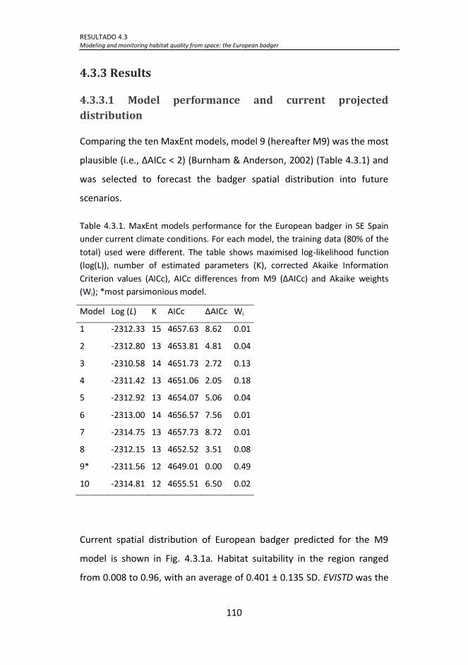
RESULTADO 4.3 Modeling and monitoring habitat quality from space: the European badger
110
4.3.3 Results
4.3.3.1 Model performance and current projected
distribution
Comparing the ten MaxEnt models, model 9 (hereafter M9) was the most
plausible (i.e., ∆AICc < 2) (Burnham & Anderson, 2002) (Table 4.3.1) and
was selected to forecast the badger spatial distribution into future
scenarios.
Table 4.3.1. MaxEnt models performance for the European badger in SE Spain
under current climate conditions. For each model, the training data (80% of the
total) used were different. The table shows maximised log-likelihood function
(log(L)), number of estimated parameters (K), corrected Akaike Information
Criterion values (AICc), AICc differences from M9 (∆AICc) and Akaike weights
(Wi); *most parsimonious model.
Model Log (L) K AICc ∆AICc Wi
1 -2312.33 15 4657.63 8.62 0.01
2 -2312.80 13 4653.81 4.81 0.04
3 -2310.58 14 4651.73 2.72 0.13
4 -2311.42 13 4651.06 2.05 0.18
5 -2312.92 13 4654.07 5.06 0.04
6 -2313.00 14 4656.57 7.56 0.01
7 -2314.75 13 4657.73 8.72 0.01
8 -2312.15 13 4652.52 3.51 0.08
9* -2311.56 12 4649.01 0.00 0.49
10 -2314.81 12 4655.51 6.50 0.02
Current spatial distribution of European badger predicted for the M9
model is shown in Fig. 4.3.1a. Habitat suitability in the region ranged
from 0.008 to 0.96, with an average of 0.401 ± 0.135 SD. EVISTD was the

RESULTADO 4.3 Modeling and monitoring habitat quality from space: the European badger
111
most important variable based on the jackknife test using the regularized
training gain; EVISTD caused the highest gain when used alone in the
model, and the greatest decrease in gain when removed from the model
(Table 4.3.2). However, using the regularized test gain, EVISTD also
achieved the highest gain when used alone, but PREC caused the greatest
decrease in gain when removed from the model.
Table 4.3.2. Most important environmental variables (*) in the MaxEnt model
for habitat suitability of the European badger in SE arid Spain under current
climate conditions (1971-2000). Relative importance of variables was evaluated
by a jackknife test on the training and test gains. The gains obtained using all
variables were 0.227 for training data and 0.397 for test data, so these were the
reference values. (see “Environmental variables” subsection for variables
abbreviations).
Training gain Test gain
Variable With only Without With only Without
PREC 0.042 0.193 0.007 0.276*
TMEDMAX 0.075 0.211 -0.051 0.435
SLOPE 0.028 0.192 0.001 0.334
EVIMEAN 0.038 0.206 0.161 0.285
EVICV 0.006 0.205 0.057 0.348
EVISTD 0.111* 0.170* 0.204* 0.30
The correlations between habitat suitability in the presence records and
each environmental variable under current conditions suggest which
environmental factors influence the presence of European badger. Thus,
EVISTD and TMEDMAX had the two highest positive values (Table 4.3.3),
while PREC and EVICV reached the two highest negative values.

RESULTADO 4.3 Modeling and monitoring habitat quality from space: the European badger
112
Table 4.3.3. Pearson coefficient correlation (rho) between habitat suitability
predicted in the presence records under current climate conditions (1971-2000),
and each environmental variable. (*P < 0.05; **P < 0.001). (see “Environmental
variables” subsection for variables abbreviations).
Variable rho
PREC -0.49**
TMEDMAX 0.56**
SLOPE -0.18*
EVIMEAN 0.15*
EVICV -0.25**
EVISTD 0.73**
4.3.3.2 Forecasted future distributions
MaxEnt model M9 forecasted a decrease in high habitat suitability sites
for the European badger in the arid region of SE Spain under both A2 and
B1 future climate scenarios (Fig. 4.3.1a). The sites with high habitat
suitability (> 0.67) completely disappeared under both scenarios
(suitability ranged from 0.009 to 0.67 (A2) and 0.62 (B1)), changing the
skewness of the habitat suitability values from 0.40 (current) to -0.64
(A2) and -0.54 (B1) (skewness was estimated using the type 3 method in
Joanes & Gill, 1998). However, the average of habitat suitability for the
study area were similar (current conditions: 0.40 ± 0.13 SD; A2: 0.43 ±
0.11 SD and B1: 0.39 ± 0.11 SD). Therefore, the I similarity statistic
showed a low difference between current and forecasted future
distributions (0.93 and 0.92 for A2 and B1 respectively), which means a
high similitude between spatial distributions at regional scale.
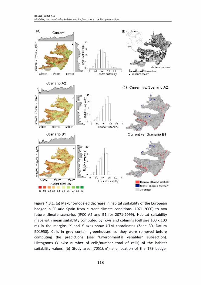
RESULTADO 4.3 Modeling and monitoring habitat quality from space: the European badger
113
Figure 4.3.1. (a) MaxEnt-modeled decrease in habitat suitability of the European
badger in SE arid Spain from current climate conditions (1971-2000) to two
future climate scenarios (IPCC A2 and B1 for 2071-2099). Habitat suitability
maps with mean suitability computed by rows and columns (cell size 100 x 100
m) in the margins. X and Y axes show UTM coordinates (Zone 30, Datum
ED1950). Cells in grey contain greenhouses, so they were removed before
computing the predictions (see “Environmental variables” subsection).
Histograms (Y axis: number of cells/number total of cells) of the habitat
suitability values. (b) Study area (7051km2) and location of the 179 badger

RESULTADO 4.3 Modeling and monitoring habitat quality from space: the European badger
114
presence records used in this study. The area only includes arid climate; based
on Martonne aridity index. (c) MaxEnt-modeled maps of significant differences
in habitat suitability between current and predicted climate conditions under
the A2 and B1scenarios for the European badger in SE arid Spain. In pale red,
areas where the variables are expected to significantly decrease (SD > 0.975); in
blue, areas where the variables are expected to significantly increase (SD <
0.025); and in grey, areas where there was no significant difference.
4.3.3.3 Potential areas to lose habitat suitability and
involved environmental drivers
The MaxEnt model M9 revealed more loss than gain of suitable habitats
for the European badger in SE Spain under both A2 and B1 climate
change scenarios. Habitat suitability is expected to significantly decrease
in both scenarios: A2 by 3.85% and B1 by 4.04 % of the study area. In
both scenarios, significant decreases occurred along the two main river
valleys and along the eastern coastline (Fig. 4.3.1c). In contrast, some
areas are also expected to significantly gain habitat suitability in both
scenarios (though with lower extension than losses): A2 by 1.32% and B1
by 1.15%. In both scenarios, significant gains occurred in the central and
northwestern parts of the study area.
According to MaxEnt model M9 under current climate conditions, the
main limiting factor of habitat suitability for the European badger in SE
Spain strongly varied across the region (Fig. 4.3.2) Slope was important in
mountains, as well as precipitation (PREC) and temperature (TMEDMAX),
particularly in inner mountains. The EVI descriptors of temporal and
spatial patterns of ecosystem functioning (i.e., EVIMEAN, EVICV and
EVISTD) were more limiting at low-altitude foothills, plains and valleys.
Conversely, under both future climate scenarios, the spatial standard
deviation of EVIMEAN (EVISTD) was the main limiting factor throughout
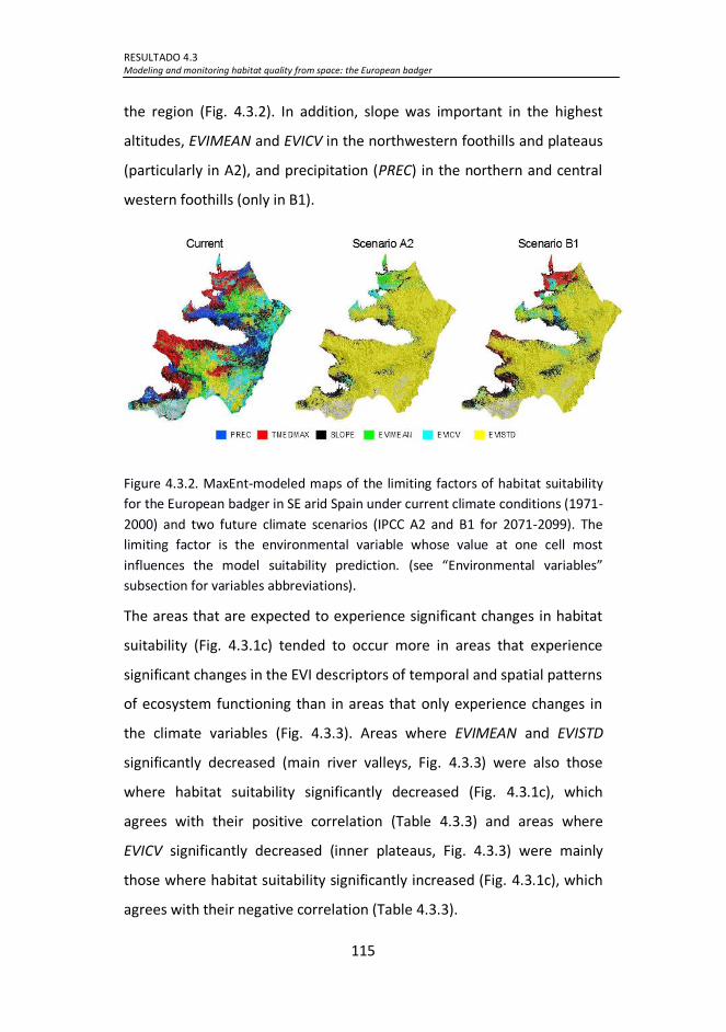
RESULTADO 4.3 Modeling and monitoring habitat quality from space: the European badger
115
the region (Fig. 4.3.2). In addition, slope was important in the highest
altitudes, EVIMEAN and EVICV in the northwestern foothills and plateaus
(particularly in A2), and precipitation (PREC) in the northern and central
western foothills (only in B1).
Figure 4.3.2. MaxEnt-modeled maps of the limiting factors of habitat suitability
for the European badger in SE arid Spain under current climate conditions (1971-
2000) and two future climate scenarios (IPCC A2 and B1 for 2071-2099). The
limiting factor is the environmental variable whose value at one cell most
influences the model suitability prediction. (see “Environmental variables”
subsection for variables abbreviations).
The areas that are expected to experience significant changes in habitat
suitability (Fig. 4.3.1c) tended to occur more in areas that experience
significant changes in the EVI descriptors of temporal and spatial patterns
of ecosystem functioning than in areas that only experience changes in
the climate variables (Fig. 4.3.3). Areas where EVIMEAN and EVISTD
significantly decreased (main river valleys, Fig. 4.3.3) were also those
where habitat suitability significantly decreased (Fig. 4.3.1c), which
agrees with their positive correlation (Table 4.3.3) and areas where
EVICV significantly decreased (inner plateaus, Fig. 4.3.3) were mainly
those where habitat suitability significantly increased (Fig. 4.3.1c), which
agrees with their negative correlation (Table 4.3.3).

RESULTADO 4.3 Modeling and monitoring habitat quality from space: the European badger
116
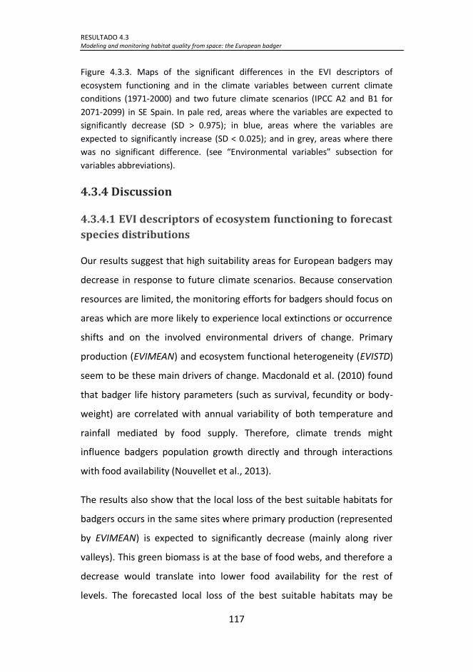
RESULTADO 4.3 Modeling and monitoring habitat quality from space: the European badger
117
Figure 4.3.3. Maps of the significant differences in the EVI descriptors of
ecosystem functioning and in the climate variables between current climate
conditions (1971-2000) and two future climate scenarios (IPCC A2 and B1 for
2071-2099) in SE Spain. In pale red, areas where the variables are expected to
significantly decrease (SD > 0.975); in blue, areas where the variables are
expected to significantly increase (SD < 0.025); and in grey, areas where there
was no significant difference. (see “Environmental variables” subsection for
variables abbreviations).
4.3.4 Discussion
4.3.4.1 EVI descriptors of ecosystem functioning to forecast
species distributions
Our results suggest that high suitability areas for European badgers may
decrease in response to future climate scenarios. Because conservation
resources are limited, the monitoring efforts for badgers should focus on
areas which are more likely to experience local extinctions or occurrence
shifts and on the involved environmental drivers of change. Primary
production (EVIMEAN) and ecosystem functional heterogeneity (EVISTD)
seem to be these main drivers of change. Macdonald et al. (2010) found
that badger life history parameters (such as survival, fecundity or body-
weight) are correlated with annual variability of both temperature and
rainfall mediated by food supply. Therefore, climate trends might
influence badgers population growth directly and through interactions
with food availability (Nouvellet et al., 2013).
The results also show that the local loss of the best suitable habitats for
badgers occurs in the same sites where primary production (represented
by EVIMEAN) is expected to significantly decrease (mainly along river
valleys). This green biomass is at the base of food webs, and therefore a
decrease would translate into lower food availability for the rest of
levels. The forecasted local loss of the best suitable habitats may be

RESULTADO 4.3 Modeling and monitoring habitat quality from space: the European badger
118
driven by lower food availability under a new scenario of increasing
aridity. This will likely translate to changes in regional distribution,
abundance and life-history traits (such as fitness or body-weight).
In addition, the local loss of the best suitable habitats for badgers occurs
in the same sites where the spatial heterogeneity of primary production
(represented by EVISTD) is expected to significantly decrease under
future climate scenarios. At the regional scale, they also display that
EVISTD is expected to become the main limiting factor of habitat
suitability throughout the study area. In the arid Mediterranean climate,
badgers prefer to live in rural landscapes consisting in a mosaic of fruit
crops and orchards mixed with patches of semi-natural vegetation,
where the heterogeneity provides diverse food resources and shelters
(Lara-Romero et al. 2012). Several authors have suggested that this
preference is a response to food shortage (Lara-Romero et al., 2012;
Requena-Mullor et al., 2014). Mosaic landscapes represent a predictable,
clumped and profitable habitat to maximize the regional stability of food
supply such as fruits, insects or vertebrates in an arid region. In this way,
badgers would offset the lower availability of key prey items (i.e.,
earthworms) in arid regions compared to more rainy regions within its
distribution range (Kruuk, 1978). The forecasted landscape
homogenization in terms of ecosystem functioning would imply a
decrease in habitat suitability.
Conversely, our study also revealed some new spots that would reach
moderately high habitat suitability (from 0.5 to 0.7) under future climate
change scenarios. In such areas, the intra-annual variability of primary
production (seasonal coefficient of variation of EVI; EVICV) is expected to
significantly decrease. EVICV has been used as an indicator of carbon

RESULTADO 4.3 Modeling and monitoring habitat quality from space: the European badger
119
gains seasonality that describes the variability of green biomass
production across seasons (Alcaraz-Segura et al., 2009). At the European
scale, badger densities are known to be limited by seasonal temperature,
or some other constraint(s) that covary with seasonality (Johnson et al.,
2002). At the local scale, it is also known that badger survival is especially
sensitive to seasonal weather extremes, such as extended summer
droughts and winter frosts (Macdonald & Newman 2002). For instance,
Woodroffe & Macdonald (2000) found that summer rainfall is a
significant predictor of cub survivorship. In SE Spain, seasonality is
expected to increase due to increasing temperatures and decreasing
rainfall, particularly during summer months (De Luis et al., 2001). Greater
seasonality would lead to lower habitat quality for badgers, monitoring
and management actions should pay special attention to such critical
periods that increase seasonality of primary production. However, for
monitoring purposes, it is important to bear in mind that changes in
primary production may be time-lagged with regard to changes in
precipitation or temperature (Cabello et al., 2012b). For example, in the
study area, Cabello et al. (2012b) observed from 2000 to 2010 that slight
precipitation increases during late summer led to relatively much higher
EVI increases in late autumn, which persisted throughout the winter
(critical periods in badger population dynamics, Macdonald et al., 2010).
Our results highlight seasonality of primary production, but not
seasonality of precipitation or temperatures, to better determine habitat
suitability for badgers, so focusing solely on weather extremes is not
enough for an effective monitoring of badgers populations in the study
area.

RESULTADO 4.3 Modeling and monitoring habitat quality from space: the European badger
120
4.3.4.2 Global and local implications for wildlife monitoring
and management
One of the strategies suggested to adapt species monitoring and
management to climate change is evaluating and enhancing monitoring
programs for wildlife on a global scale (Mawdsley et al., 2009). However,
the costs to adapt existing monitoring systems are likely to be high.
Therefore new tools and approaches are required. Here we show that
cost-efficient monitoring schemes using globally available data sets (i.e.,
variables related to ecosystem functional attributes derived from remote
sensing) are sensitive to both long-term and rapid environmental
changes affecting the distribution range of a species (Crabtree et al.,
2009).
At the local scale of our study, the arid Mediterranean rural landscape is
a shifting mosaic that benefits carnivore diversity and abundance (Pita et
al., 2009). In this challenging environment, monitoring of future
landscape trajectories is vital for biodiversity conservation and
maintaining connectivity between suitable habitat areas (Piquer-
Rodríguez et al., 2012). Our results suggest to local managers that EVI-
derived functional attributes are useful to detect priority areas for
monitoring based on their loss or gain habitat suitability for badgers. For
instance, the areas where EVIMEAN significantly decreased were also
those where habitat suitability significantly decreased, which suggest
monitoring the spatial and temporal variability of EVI functional
attributes detects changes in habitat suitability. Likewise, seasonal
dynamic of primary production (represented by EVICV) could allow to
identify critical periods where focus the monitoring actions. These results
enhance previous findings by Requena-Mullor et al. (2014), which

RESULTADO 4.3 Modeling and monitoring habitat quality from space: the European badger
121
showed that the distribution of European badgers in this region was
predicted by functional attributes such as high primary production
(EVIMEAN), seasonality in the primary production (EVICV) and spatially
heterogeneous landscapes (EVISTD). However, advances in the
knowledge of the relationship between these functional attributes and
food resources availability are still necessary for effective monitoring of
the European badger.
In conclusion, the incorporation of ecosystem functional attributes
derived from remote sensing in the modeling of future forecast may
contribute to the improvement of the detection of ecological responses.
We believe that our approach can be applied in a variety of ecosystems
worldwide and under diverse climatic change scenarios, thereby
supporting the design of optimized/cost-efficient monitoring schemes.
The use of predictive models, such as ours, can address and improve the
ever-increasing need for monitoring of biodiversity across space and time
in a rapidly changing planet.

DISCUSIÓN
122
5. DISCUSIÓN
El Tejón europeo se enfrenta a una serie de amenazas que pueden poner
en jaque la viabilidad de sus poblaciones, o en última instancia, su
presencia en los ecosistemas Mediterráneos a finales del siglo XXI. Esta
situación se agrava en algunos paisajes áridos Mediterráneos, donde la
especie es poco abundante y con distribución parcheada, lo cual hace su
supervivencia aún más complicada. Entre las amenazas más destacadas
se encuentran el cambio climático, consecuencia del calentamiento
atmosférico global, y la pérdida-fragmentación de su hábitat, ocasionada
por los cambios en el uso y la cobertura del suelo (Virgós et al., 2005c).
Varios trabajos han destacado los efectos potenciales que las variaciones
en los ciclos de precipitación y temperatura tienen sobre la dinámica
poblacional del Tejón (Macdonald et al., 2010; Nouvellet et al., 2013). Sin
embargo, la respuesta de la especie puede variar de unas regiones a
otras, por lo que se requieren estudios en diferentes áreas de su rango
de distribución (Virgós et al., 2005c). Por otro lado, el ser humano está
modificando la composición del paisaje y sustituyendo las prácticas
agrícolas tradicionales por otras más intensivas y menos respetuosas con
el entorno (Pita et al., 2009). Por este motivo, y dado que los paisajes
rurales Mediterráneos son el hábitat preferido del Tejón en ambientes
áridos, la calidad de su hábitat, y por tanto, la abundancia de la especie,
podría verse significativamente reducida (Lara-Romero et al., 2012).
En relación a esto, el último informe del Panel Intergubernamental
contra el Cambio Climático es claro: sin una gestión eficaz, derivada de
políticas de conservación que tengan en cuenta los efectos potenciales
del Cambio Global, algunas especies en riesgo menor en la actualidad,
pueden llegar a ser mucho más raras, e incluso desaparecer localmente

DISCUSIÓN
123
durante el siglo XXI (IPCC, 2013; Inger et al., 2015). La pérdida de
especies puede llevar a su vez a una reducción local de la biodiversidad y
a una modificación de la estructura y funcionamiento del ecosistema
(National Research Council, 1999). De forma particular, los meso-
carnívoros como el Tejón, juegan un papel relevante en los sistemas
naturales como predadores, competidores y especies “paragua”. De este
modo, variaciones en su abundancia o en la diversidad de sus
comunidades pueden inducir cambios a nivel ecosistema (Roemer et al.,
2009). Todo ello pone de manifiesto la necesidad de mejorar el
conocimiento sobre el rango actual de distribución del Tejón y los efectos
potenciales que sobre el mismo pudiera tener el Cambio Global. De esta
forma, los gestores pueden optimizar las medidas de conservación y
diseñar programas de seguimiento más eficientes, no solo de cara a la
conservación de la especie, sino también de los paisajes que habita
(Proyecto GLOCHARID, 2014).
Esta tesis doctoral supone un avance en esta línea de trabajo, y propone
algunas recomendaciones para el seguimiento de su distribución y
conservación del hábitat en un contexto Mediterráneo árido.
Uno de los principales impulsores de la distribución espacial del Tejón en
paisajes áridos Mediterráneos es la dinámica espacio-temporal de la
producción primaria (Requena-Mullor et al., 2014) (ver RESULTADO 4.1).
La producción primaria está situada en la base de la cadena trófica y
sintetiza aspectos funcionales clave de los ecosistemas, por lo que es
considerada un atributo integrador del funcionamiento ecosistémico
(McNaughton et al., 1989; Virginia & Wall, 2001). En un planeta que
cambia rápidamente, disponer de herramientas que informen casi a
tiempo real de la dinámica de la producción vegetal resulta de vital

DISCUSIÓN
124
importancia en tareas de seguimiento ecológico. En la era de los
satélites, la traslación de la información espectral a variables
relacionadas con el funcionamiento ecosistémico está ampliando el uso
tradicional de las imágenes de satélite en la biología de la conservación,
ofreciendo descriptores de procesos clave del funcionamiento de los
ecosistemas (ej., dinámica de la producción primaria, evapotranspiración,
eficiencia en el uso del agua por la vegetación, etc.) (Cabello et al., 2012).
Estos descriptores están resultando muy valiosos a la hora de modelizar
rasgos de la ecología de las especies y su respuesta frente a los cambios
ambientales (Cabello et al., 2012a). Un ejemplo de ello son los atributos
funcionales derivados de índices de vegetación, tales como el EVI. Estos
atributos son sensibles a factores que afectan al rango de distribución de
las especies (Crabtree et al., 2009), y han resultado de gran utilidad en la
modelización de la distribución espacial del Tejón europeo (Requena-
Mullor et al., 2014).
De cara al reto de monitorear los efectos que el Cambio Global pueda
tener sobre la distribución de la especie es indudable que resulta
determinante el uso de información satelital relacionada con la
producción primaria. Bajo la asunción de que la producción vegetal de un
área influencia la red trófica completa (McNaughton et al., 1989), los
atributos funcionales pueden ayudar a comprender (de abajo a arriba) las
alteraciones en la dinámica de las comunidades como respuesta a los
cambios ambientales. Frente al cambio climático, esta visión puede
resultar particularmente útil en ambientes Mediterráneos, debido a que
la precipitación es el principal factor limitante del crecimiento vegetal
(Nemani et al., 2003) (ver RESULTADO 4.3). La respuesta rápida de estos
atributos frente a cambios ambientales, su disponibilidad en continuo,
DISCUSIÓN
125
espacial y temporal a resoluciones óptimas regionales, hacen de ellos
una herramienta muy eficaz en el estudio y seguimiento de la
distribución de las especies.
Es importante resaltar que el uso de imágenes satelitales para derivar
atributos funcionales requiere de un filtrado previo de calidad de las
mismas (Reyes et al., 2015) y de una normalización-estandarización de
los algoritmos empleados en la estima de los mismos. Todo ello pone de
manifiesto la necesidad de protocolos internacionales consensuados que
permitan extender su uso a escalas más amplias y poder comparar los
resultados entre distintas áreas del planeta. De esta forma, avances en
distintos ámbitos de conocimiento y ecosistemas del planeta pueden
integrarse y servir de apoyo en la búsqueda de criterios generales sobre
los que apoyar Normas y Directrices internacionales en la lucha contra el
Cambio Global y la pérdida de biodiversidad.
Si analizamos el caso concreto del Tejón en el contexto árido
Mediterráneo, la dinámica espacio-temporal de la producción primaria
condiciona en gran medida su distribución espacial. Este resultado
(RESULTADO 4.1) hace pensar que existe algún tipo de correlación entre
los atributos funcionales que describen dicha distribución y la dinámica
espacio-temporal de los recursos alimenticios explotados por la especie.
El Tejón selecciona áreas con altos valores de producción vegetal y
heterogeneidad espacial, mientras que rechaza zonas con alta
variabilidad temporal en dicha producción. Estas condiciones suelen ser
representativas de paisajes rurales tradicionales bien conservados que
ofrecen al Tejón una oferta de recursos alimenticios variada
espacialmente y estable a lo largo del año (Requena-Mullor et al., 2014).

DISCUSIÓN
126
Sin embargo, poco se sabe de la relación entre la dinámica espacio-
temporal de los atributos funcionales del EVI y los recursos alimenticios
explotados por el Tejón. De entre los ítems consumidos por la especie en
ambientes Mediterráneos, son especialmente importantes los frutos,
insectos y vertebrados (Rodríguez & Delibes, 1992; Revilla & Palomares,
2002; Barea-Azcón et al., 2010, Requena-Mullor et al., 2015). Algunas de
las cuestiones a responder en relación a esto son: ¿hay una relación
directa positiva entre la producción primaria y la disponibilidad de
frutos?, ¿existe desfase temporal entre la fenología de la producción
vegetal y la disponibilidad de alimento?, y en caso afirmativo, ¿cuál es su
magnitud?, y ¿un paisaje heterogéneo, ofrece realmente una oferta más
variada de alimento?. En esta dirección, algunos autores han relacionado
la ocurrencia o abundancia de estos ítems con índices de vegetación tales
como el EVI o el Índice de Vegetación de Diferencia Normalizada (del
inglés, NDVI) (Willems et al., 2009; Lafage et al., 2013; Tapia et al., 2013),
pero poco más se sabe.
Para seguir avanzando en esta línea es imprescindible identificar primero
qué recursos alimenticios explota el Tejón, y si existe variabilidad en las
estrategias tróficas adoptadas entre paisajes dentro de un contexto árido
Mediterráneo. En este sentido, los resultados encontrados muestran
cómo los hábitos alimenticios del Tejón varían de unos paisajes a otros
dentro del contexto árido (ver RESULTADO 4.2). Aunque la frugivoría
sigue apareciendo como la principal estrategia adoptada por la especie
(Pigozzi, 1991; Rodríguez & Delibes, 1992; Barea-Azcón et al., 2010), en
zonas montañosas, donde la repoblación con pinos es el rasgo
dominante del paisaje, los invertebrados (ej., insectos y lombrices)
adquieren una importancia significativa. Este aumento en el consumo de

DISCUSIÓN
127
invertebrados compensaría la escasez de frutos cultivados y/o silvestres
de mayor contenido energético (ej., naranjas, aceitunas, higos,
algarrobas, etc.), los cuales son más abundantes en las vegas fluviales y
matorrales de la maquia mediterránea situados a menor altitud.
La dependencia directa y/o indirecta del Tejón hacia el manejo que el ser
humano hace del territorio se pone de manifiesto cuando se analizan sus
hábitos alimenticios. De esta forma, las prácticas agrícolas tradicionales
aportan a la especie no solo frutos cultivados (ej., naranjas), sino otros
como higos, nísperos, manzanas, albaricoques, etc., cultivados
secundariamente o en muchos casos naturalizados, pero dependientes
en cierto grado del regadío (Requena-Mullor et al., 2015). Además,
debido al escaso uso de pesticidas y maquinaria agrícola, esto ambientes
pueden ofrecer una gran diversidad y abundancia de artrópodos
(Bengtsson et al., 2005). Por todo ello, es importante tener en cuenta el
efecto potencial de las políticas agrarias sobre una especie como el
Tejón, en cuanto que pueden ser impulsoras de cambios en el uso del
suelo (Virgós et al., 2005c). En este sentido, la reforma de la Política
Agraria Común (PAC) para el período 2014-2020, contempla un paquete
de medidas que promueven la diversificación de cultivos, mantenimiento
de pastos permanentes y el destino de parte de la propiedad como
superficie de interés ecológico (Martínez & Palacios, 2012). Estas
prácticas, favorecerían a priori la conservación de las poblaciones de
Tejón en ambientes Mediterráneos (Virgós et al., 2005c), sin embargo, el
envejecimiento de la población rural y el éxodo de los más jóvenes a las
ciudades está propiciando un abandono generalizado de tierras en las
últimas décadas (Castro et al., 2011). Esto trae consigo un deterioro del
DISCUSIÓN
128
paisaje rural Mediterráneo, y por tanto, una amenaza para el futuro de la
especie.
Por otro lado, algunos ítems consumidos por el Tejón dependen
directamente de la precipitación, (ej., algarrobas, palmitos, moras,
lombrices), o indirectamente de la producción primaria (ej., insectos,
roedores, conejos). Ante un escenario de cambio climático futuro, la
disponibilidad de estos recursos, o la modificación de su fenología,
podría tener consecuencia en sus hábitos alimenticios, adaptándolos a la
nueva situación (Virgós et al., 2004). En casos de periodos extremos de
aridez, podría verse obligado a abandonar el territorio y buscar nuevas
zonas, lo que en condiciones de distribución parcheada, puede
incrementar el riesgo de desaparición local (Virgós et al., 2005c). En
relación a esto último, la calidad del hábitat para el Tejón en paisajes
áridos Mediterráneos podría verse significativamente reducida de aquí a
finales de siglo (ver RESULTADO 4.3). No obstante, esta reducción no
sería uniforme en el espacio, pudiendo incluso aumentar en algunas
zonas. Aquellas que ofrecen en la actualidad las mejores condiciones
para la supervivencia del Tejón (esto es, los paisajes agrícolas
tradicionales (Lara-Romero et al., 2012)), verían reducida su idoneidad de
hábitat debido principalmente a una homogeneización del paisaje desde
el punto de vista de la producción primaria. Por el contrario, algunas
áreas del centro y norte del área de estudio, aunque de menor extensión,
aumentarían su idoneidad gracias a una disminución en la estacionalidad
de la producción primaria. A pesar de que estos resultados hay que
tomarlos con precaución, debido a que no se tienen en cuenta de
manera directa los cambios en el uso del suelo (Pearson & Dawson,
2003) y la incertidumbre asociada a los modelos climáticos (Deser et al.,

DISCUSIÓN
129
2012), otros autores predicen igualmente una homogeneización del
paisaje derivada de la intensificación de los cultivos, y a un abandono del
uso agrícola tradicional ocasionado por el éxodo humano a áreas urbanas
(Silvestre, 2002; De Stefano, 2004; Piquer-Rodríguez et al., 2012). Por
tanto, estas previsiones dibujarían igualmente un escenario poco
alentador para la especie. De hecho, Maiorano et al. (2014) predicen, en
base a los mismos escenarios de cambio y período de tiempo que los
empleados en esta tesis doctoral, una disminución de hasta un 50% en la
distribución de las especies de la familia Mustelidae en la cuenca
Mediterránea. En un contexto global cambiante, el último informe del
IPCC para la conservación de los mamíferos predice que el 25% de las
especies de mamíferos del mundo, aproximadamente unas 1,125
especies, están en riesgo de extinción global (IPCC, 2013). Paralelamente,
Inger et al. (2015) alertan de que las especies que en la actualidad no
están amenazas corren serio peligro de estarlo en el futuro debido a que
toda la atención se centra en aquellas que sí lo están.
Desde esta perspectiva, resulta de vital importancia para la conservación
del Tejón en ambientes áridos Mediterráneos el seguimiento y
preservación de la calidad de su hábitat de cara a prever un potencial
deterioro y por tanto, un retroceso en su rango de distribución. Por ello,
son claves las iniciativas encaminadas al mantenimiento del paisaje rural
Mediterráneo. Las nuevas políticas en materia de conservación a nivel
nacional e internacional en los países Mediterráneos donde el Tejón está
presente deberían centrar esfuerzos en la protección y conservación de
dichos paisajes, e incluir los atributos funcionales derivados de sensores
remotos como herramienta para la caracterización y seguimiento del
estado de conservación (Proyecto GLOCHARID, 2014). Dichas políticas

DISCUSIÓN
130
deben contemplar acciones a llevar a cabo tanto dentro como fuera de
las áreas naturales protegidas debido a que una gran proporción de estos
paisajes se encuentran fuera de dichos límites (Cox & Underwood, 2011).
Una de las estrategias propuestas es el desarrollo de medidas
específicamente diseñadas para prevenir el abandono rural y preservar
las tierras agrícolas (Falcucci et al., 2007). Por un lado, el éxodo humano
de los entornos rurales a la ciudad debe de frenarse con programas que
estimulen las oportunidades de futuro, y por otro lado, medidas
orientadas a mantener la heterogeneidad paisajística y las prácticas
agrícolas tradicionales, ayudarían a preservar la biodiversidad asociada a
los agro-ecosistemas Mediterráneos. Por último, es imprescindible
aplicar de manera eficaz y rigurosa la normativa que rige la ordenación
del territorio y regula los cambios en el uso del suelo para evitar la
intensificación de los cultivos y la homogeneización del paisaje.

CONCLUSIONES
131
6. CONCLUSIONES
1. Los descriptores del funcionamiento ecosistémico, obtenidos a partir
de información satelital, representan una herramienta útil e innovadora
en la modelización de la distribución espacial de meso-carnívoros como
el Tejón europeo. Esto reafirma la necesidad de poner a disposición de
gestores y tomadores de decisiones herramientas que incorporen esta
información para elaborar e implementar programas de seguimiento
como parte de estrategias orientadas a la conservación de la
biodiversidad.
2. Los resultados obtenidos identifican las huertas tradicionales como
uno de los paisajes clave para la supervivencia del Tejón europeo en
paisajes áridos Mediterráneos. Dentro de un termoclima árido, esta tesis
sugiere que los cambios en la dinámica de la precipitación y/o la
modificación del paisaje pueden ejercer efectos sobre los hábitos
alimenticios del Tejón europeo, pudiendo en última estancia poner en
jaque la viabilidad de sus poblaciones a finales del siglo XXI.
3. El debate abierto asociado a que especies no amenazadas en la
actualidad podrían estarlo en el futuro pone de manifiesto la necesidad
de políticas de conservación que incorporen una visión de la
biodiversidad más general, sin particularizar tanto en especies
“emblemáticas”.
4. Finalmente, esta tesis representa un ejemplo de la aplicabilidad de las
técnicas de muestreo tradicional de mamíferos combinado con el uso de
información satelital en el estudio de procesos claves en la biología de la
especies.

REFERENCIAS
132
REFERENCIAS
Agencia Andaluza del Agua. (2010). Río Andarax. Agencia Andaluza del
Agua. Consejería de Medio Ambiente (Editores). Junta de Andalucía.
Sevilla.
Agresti, A. (1996). An Introduction to Categorical Data Analysis. Wiley,
New York.
Alcaraz-Segura, D. (2005). Caracterización mediante teledetección del
funcionamiento de los ecosistemas ibéricos. Bases para la conservación
de la biodiversidad en un escenario de cambio global. (Tesis doctoral
inédita). Universidad de Almería. Almería.
Alcaraz-Segura, D., Paruelo, J.M. & Cabello J. (2006). Identification of
current distribution of Ecosystem Functional Types in the Iberian
Peninsula. Global Ecology and Biogeography, 15(2):200–210.
Alcaraz-Segura, D., Cabello, J. & Paruelo, J. (2009). Baseline
characterization of major Iberian vegetation types based on the NDVI
dynamics. Plant Ecology, 202:13-29.
Alcaraz-Segura, D., Paruelo, J.M., Epstein, H.E. & Cabello, J. (2013).
Environmental and Human Controls of Ecosystem functional Diversity in
Temperate South America. Remote sensing, 5(1):127-154.
Amorin, F., Carvalho, S.B., Honrado, J. & Rebelo H. (2014). Designing
Optimized Multi-Species Monitoring Networks to Detect Range Shifts
Driven by Climate Change: A Case Study with Bats in the North of
Portugal. PLOS ONE, 9, e87291. doi:10.1371/journal.pone.0087291.

REFERENCIAS
133
Andalusia Land use/Land cover map (scale 1:25.000). (2007). Disponible
en http://www.juntadeandalucia.es/medioambiente/site/rediam.
Araújo, M.B. & Peterson, A.T. (2012). Uses and misuses of bioclimatic
envelope modeling. Concepts & Synthesis, 93:1527-1539.
Armas, C., Miranda, J. D., Padilla, F. M. & Pugnaire, F. I. (Editores). (2011).
Special issue: The Iberian Southeast. Journal of Arid Environments,
75:1241-1243.
Austin, M. (2007). Species distribution models and ecological theory: A
critical assessment and some possible new approaches. Ecological
Modelling, 200:1-19.
Bardsen, B.J. & Tveraa, T. (2012). Density-dependence vs. density-
independence - linking reproductive allocation to population abundance
and vegetation greenness. Journal of Animal Ecology, 81:364-376.
Barea-Azcón, J.M., Ballesteros-Duperón, E., Gil-Sánchez, J.M. & Virgós, E.
(2010). Badger Meles meles feeding ecology in dry Mediterranean
environments of the southwest edge of its distribution range.
ActaTheriologica. 55(1):45-52.
Bateman, B.L., VanDerWal, J., Williams, S.E. & Johnson, C.N. (2012).
Biotic interactions influence the projected distribution of a specialist
mammal under climate change. Diversity and Distributions, 18:861-872.
Bengtsson, J., Ahnström, J. & Weibull, A. (2005). The effects of organic
agriculture on biodiversity and abundance: a meta-analysis. Journal of
Applied Ecology, 42(2):261-269.

REFERENCIAS
134
Best, D. J. & Roberts, D. E. (1975). The Upper Tail Probabilities of
Spearman's rho. Journal of the Royal Statistical Society. Series C (Applied
Statistic), 24:377–379.
Blanco, J. C. & González, J. L. (1992). Libro Rojo de los Vertebrados de
España. ICONA, Ministerio de Agricultura, Pesca y Alimentación, Madrid,
España, 714 p.
Booth, G.D., Niccolucci, M.J. & Schuster, E.G. (1994). Identifying proxy
sets in multiple linear regression: an aid to better coefficient
interpretation. Intermountain Research Station, USDA Forest Service,
Ogden, Utah, USA.
Boyce, M.S. (1978). Climatic variability and body size variation in the
muskrast (Ondatra zibethicus) of North America. Oecologia, 36:1-19.
Brown, J.H., Mehlman, D.W. & Steven, G.C. (1995). Spatial variance in
abundance. Ecology, 76:2028-2043.
Buermann, W., Saatchi, S., Smith, T.B., Zutta, B.R., Chaves, J.A., Milá, B. &
Graham, C.H. (2008). Prediction species distributions across the
Amazonian and Andean regions using remote sensing data. Journal of
Biogeography 35(7):1160-1176.
Burnham, K.P. & Anderson, D.R. (2002). Model selection and multimodel
inference. A practical information-theoretic approach. Springer-Verlag.
New York.
Cabello, J., Fernández, N., Alcaraz-Segura, D., Oyonarte, C., Piñeiro, G.,
Altesor, A., Delibes, M. & Paruelo, J.M. (2012a). The ecosystem
functioning dimension in conservation: insights from remote sensing.
Biodiversity and Conservation, 21:3287-3305.

REFERENCIAS
135
Cabello, J., Alcaraz-Segura, D., Ferrero, R., Castro, A.J. & Liras, E. (2012b).
The role of vegetation and lithology in the spatial and inter-annual
response of EVI to climate in drylands of Southeastern Spain. Journal of
Arid Environment, 79:76-83.
Castro, A.J., Martín-López, B., García-Llorente, M., Aguilera, P.A., López,
E. & Cabello, J. (2011). Social preferences regarding the delivery of
ecosystem services in a semiarid Mediterranean region. Journal of Arid
Environment, 75(11):1201-1208.
Castro, A.J., Paruelo, J.M., Alcaraz-Segura, D., Cabello, J., Oyarzabal, M. &
López-Carrique, E. (2013). Missing gaps in the estimation of the carbon
gains service from Light Use Efficiency models. En: Alcaraz-Segura, D. &
Di Bella, C. (Editores). Earth Observation of Ecosystem Services, 105-124
p.
Chen, W., Samuelson, F.W., Gallas, B.D., Kang, L., Sahiner, B. & Petrick, N.
(2013). On the assessment of the added value of new predictive
biomarkers. BMC Medical Research Methodology, 13:98.
Ciampalini, B. & Lovari, S. (1985). Food habits and trophic niche overlap
of the badger (Meles meles L.) and the red fox (Vulpes vulpes L.) in a
Mediterranean coastal area. Z. Säugetier-Kunde, 50:226-234.
Clarke, K. R. (1993). Non-parametric multivariate analyses of changes in
community structure. Austustralian Journal of Ecology, 18:117-143.
Corbacho, C., Sánchez, J.M. & Costillo, E. (2003). Patterns of structural
complexity and human disturbance of riparian vegetation in agricultural
landscapes of a Mediterranean area. Agriculture, Ecosystems and
Environment, 95:495-507.

REFERENCIAS
136
Cox, R.L. & Underwood, E.C. (2011). The importance of Conservation
Biodiversity Outside of Protected Areas in Mediterranean Ecosystems.
PLOS ONE, 6(1):e14508.
Crabtree, R., Potter, C., Mullen, R., Sheldon, J., Huang, S., Harmsen, J.,
Rodman, A. & Jean, C. (2009). A modeling and spatio-temporal analysis
framework for monitoring environmental change using NPP as an
ecosystem indicator. Remote Sensing of Environment: 113:1486-1496.
Da Silva, J., Woodroffe, R. & Macdonald, D. W. (1993). Habitat, food
availability and group territoriality in the European badger, Meles meles.
Oecologia, 95:558-564.
Davidowitz, G. & Rosenzweig, M.L. (1998). The latitudinal gradient of
species diversity among North American grasshoppers within a single
habitat: a test of the spatial heterogeneity hypothesis. Journal of
Biogeography, 25:553-560.
De Stefano, D. (2004). Freshwater and tourism in the Mediterranean.
Rome, Italy: WWF Mediterranean Programme.
De Luis, M., García-Cano, M.F., Cortina, J., Raventós, J., González-Hidalgo,
J. C. & Sánchez, J.R. (2001). Climatic trends, disturbances and short-term
vegetation dynamics in a Mediterranean shrubland. Forest Ecology and
Management, 147(1):25-37.
Del Cerro, I., Marmi, A., Ferrando, P. & Chashchin P. (2010). Nuclear and
mitochondrial phylogenies provide evidence for four species of Eurasian
badgers (Carnivora). Zoologica Scripta, 39:415-425.
REFERENCIAS
137
DeLong, E.R., DeLong, D.M. & Clarke-Pearson, D.L. (1998). Comparing the
areas under two or more correlated receiver operating characteristic
curves: a non-parametric approach. Biometrics, 44:837-845.
Deser, C., Phillips, A., Bourdette, V. & Teng, H. (2012) Uncertainty in
climate change projections: the role of internal variability. Climate
Dynamics, 38(3-4):527-546.
Edwards, C. A. & Lofty, J. R. (1977). Biology of earthworms. Chapman and
Hall, London, U.K.
Elith, J., Graham, C.H., Anderson, R.P. Dudík, M., Ferrier, S., Guisan, A.,
Hijmans, R.J., Huettmann, F., Leathwick, J.R., Lehmann, A., Li, J.,
Lohmann, L.G., Loiselle, B.A., Manion, G., Moritz, C., Nakamura, M.,
Nakazawa, Y. & Overton, J.M., Townsend, A., Phillips, S.J., Richardson, K.,
Scachetti-Pereira, R., Schapire, R.E., Soberón, J., Williams, S., Wisz, M.S. &
Zimmermann N.E. (2006). Novel methods improve prediction of species´
distributions from occurrence data. Ecography, 29:129-151.
Elith, J. & Leathwick, J.R. (2009). Species Distribution Models: Ecological
Explanation and Prediction Across Space and Time. Annual Review of
Ecology, Evolution, and Systematics, 40:677-697.
Elith, J., Kearney, M. & Phillips, S. (2010). The art of modelling range-
shifting species. Methods in Ecology and Evolution, 1:330-342.
Elith, J., Phillips, S.J., Hastie, T., Dudík, M., Chee, Y.E. & Yates, C.J. (2011).
A statistical explanation of MaxEnt for ecologists. Diversity and
Distributions, 17:43-57.

REFERENCIAS
138
Falcucci, F., Maiorano, L. & Boitani, L. (2007). Changes in land-use/land-
cover patterns in Italy and their implications for biodiversity
conservation. Landscape Ecology, 22:617-631.
Ferguson, S.H. & McLoughlin, P.D. (2000). Effect of energy availability,
seasonality and geographic range on brown bear life history. Ecography,
23:193-200.
Feroe, S. & Montgomery, W.I. (1999). Habitat effects on the spatial
ecology of the European badger (Meles meles). Journal of Zoology,
247:537-549.
Ferrier, S. & Watson, G. (1997). An Evaluation of the effectiveness of
environmental surrogates and modeling techniques in predicting the
distribution of biological diversity. Environment Australia, Canberra
Australia. Disponible en:
http://www.environment.gov.au/archive/biodiversity/publications/techn
ical/surrogates/ .
Fischer, C., Ferrari, N. & Weber, J. M. (2005). Exploitation of food
resources by badgers (Meles meles) in the Swiss Jura Mountains. Journal
of Zoology of London, 266(2):121-131.
Fryxell, J.M., Wilmshurst, J.F., Sinclair, A.R.E., Haydon, D.T., Holt, R.D. &
Abrams, P.A. (2005). Landscape scale, heterogeneity, and the viability of
Serengeti grazers. Ecology Letters, 8:328-335.
García-Rangel, S. & Pettorelli, N. (2013). Thinking spatially: The
importance of geospatial techniques of carnivore conservation.
Ecological Informatics, 14:84-89.

REFERENCIAS
139
Giorgi, F. & Lionello, P. (2008). Climate change projections for the
Mediterranean region. Global Planet Change. 63(2-3):90-104.
Goszczynski, B., Jedrzejewska, B. & Jedrzejewski, W. (2000). Diet
composition of badgers (Meles meles) in a pristine forest and rural
habitats of Poland compared to other European populations. Journal of
Zoology of London, 250(4):495-505.
Graham, C.H. & Hijmans, R.J. (2006). A comparison of methods for
mapping species ranges and species richness. Global Ecology and
Biogeography, 15:578.
Hastie, T. & Tibshirani, R. (1990). Generalized Additive Models. Chapman
& Hall, London.
Hernández, P.A., Graham, C.H., Master, L.L. & Albert D.L. (2006). The
effect of sample size and species characteristics on performance of
different species distribution modeling methods. Ecography, 29:773-785.
Herrera, C.M. (1989). Frugivory and seed dispersal by carnivorous
mammals and associated fruit characteristics, in undisturbed
Mediterranean habitats. Oikos, 55:250-262.
Hill, M.P, Axford, J.K. & Hoffmann, A.A. (2014). Predicting the spread of
Aedes albopictus in Australia under current and future climates: Multiple
approaches and datasets to incorporate potential evolutionary
divergence. Austral Ecology, 39:469-478.
Huete, A.R., Liu, H.Q., Batchil. K. & van Leeuwen, W. (1997). A
comparison of vegetation indices global set of TM images for EOS-
MODIS. Remote Sensing of Environment, 59:440-451.

REFERENCIAS
140
Huete, A.R., Didan, K., Miura, T., Rodriguez, E.P., Gao, X. & Ferreira, L.G.
(2002). Overview of the radiometric and biophysical performance of the
MODIS vegetation indices. Remote Sensing of Environment, 83:195-213.
Inger, R., Gregory, R., Duffy, J.P., Stott, Vorïsek, P. & Gaston, K.J. (2015).
Common European birds are declining rapidly while less abundant
species’ numbers are rising. Ecology Letters, 18:28-36.
Intergovernmental Panel on Climate Change (2007) Climate Change
2007: Synthesis Report. Contribution of Working Groups I, II and III to the
Fourth Assessment Report of the Intergovernmental Panel on Climate
Change. Core Writing Team, Pachauri, R.K & Reisinger, A. (Editores). IPCC,
Geneva, Switzerland, 104 p.
IPCC, (2007): Cambio climático 2007: Informe de síntesis. Contribución de
los Grupos de trabajo I, II y III al Cuarto Informe de evaluación del Grupo
Intergubernamental de Expertos sobre el Cambio Climático [Equipo de
redacción principal: Pachauri, R.K. & Reisinger, A. (directores de la
publicación)]. IPCC, Ginebra, Suiza, 104 p.
IPCC, (2013): Climate Change 2013: The Physical Science Basis.
Contribution of Working Group I to the Fifth Assessment Report of the
Intergovernmental Panel on Climate Change. Stocker T.F., Qin G.K.
Plattner M., Tignor S.K., Allen J., Boschung A., Nauels Y., Xia V., Bex P.M.
(Editores). Cambridge University Press, Cambridge, United Kingdom and
New York, NY, USA, 1535 p.
IPCC, (2013): Summary for Policymakers. En: Climate Change 2013: The
Physical Science Basis. Contribution of Working Group I to the Fifth
Assessment Report of the Intergovernmental Panel on Climate Change.

REFERENCIAS
141
Stocker, T.F., Qin, D., Plattner, G.K., Tignor, M., Allen, S.K., Boschung, J.,
Nauels, A., Xia, Y., Bex, V. & Midgley, P.M. (Editotes). Cambridge
University Press, Cambridge, United Kingdom and New York, NY, USA, 33
p.
Januchowski, S., Pressey, B., Vanderwal, J. & Edwards, A. (2010).
Characterizing errors in topographic models and estimating the financial
costs of accuracy. International Journal of Geographical Information
Science, 24:1327-1347.
Jepsen J.U., Madsen A.B., Karlsson M. & Groth D. (2005). Predicting
distribution and density of badger (Meles meles) setts in Denmark.
Biodiversity and Conservation, 14:3235-3253.
Joanes, D.N. & Gill, C.A. (1998). Comparing measures of sample skewness
and kurtosis. The Statistician, 47:183-189.
Johnson, D.D., Jetz, W. & Macdonald, D.W. 2002. Environmental
correlates of badger social spacing across Europe. Journal of
Biogeography, 29(3):411-425.
Junta de Andalucía. (2014). El clima de Andalucía en el siglo XXI.
Consejería de Medio Ambiente y Ordenación del Territorio de la Junta de
Andalucía. (Editores). Sevilla.
Kruskal, J.B. (1964). Multidimensional scaling by optimizing goodness of
fit to a nonmetric hypotheses. Psychometrika, 29(1):1-27.
Kruuk, H. (1978). Spatial organisation and territorial behavior of the
European badger, Meles meles. Journal of Zoology, 184:1-19.

REFERENCIAS
142
Kruuk H. (1989). The social badger: ecology and behaviour of a group-
living carnivore (Meles meles). Oxford University Press.
Kruuk, H. & de Kock, L. (1981). Food and habits of badgers (Meles meles)
on Monte Baldo, northern Italy. Z. Säugetierkunde, 46:295-301.
Kruuk H. & Parish T. (1981). Feeding specialization of the European
badger Meles meles in Scotland. Journal of Animal Ecology, 50:773-788.
Kruuk, H. & Parish, T. (1985). Food, food availability and weight of
badgers (Meles meles) in relation to agricultural changes. Journal of
Applied Ecology, 22:705-715.
Lafage, D., Secondi, J., Georges, A., Bouzillé, J.B. & Pétillon, J. (2013).
Satellite-derived vegetation indices as surrogate of species richness and
abundance of ground beetles in temperate floodplains. Insect
Conservation and Diversity, doi: 10.1111/icad.12056.
Lara-Romero, C., Virgós, E., Escribano-Ávila, G., Mangas, J.G., Barja, I. &
Pardavila, X. (2012). Habitat selection by European badgers in
Mediterranean semi-arid ecosystems. Journal of Arid Environment,
76:43-48.
Lavorel, S., Canadell, J., Rambal, S. & Terradas, J. (1998). Mediterranean
terrestrial ecosystems: research priorities on global change effects.
Global Ecology and Biogeography Letters, 7:157-166.
Levinsky, I., Skov, F., Svenning J.C. & Rahbek C. (2007). Potential impacts
of climate change on the distributions and diversity patterns of European
mammals. Biodiversity and Conservation, 16:3803-3816.
REFERENCIAS
143
Lloyd, D. (1990). A phenological classification of terrestrial vegetation
cover using shortwave vegetation index imagery. International Journal of
Remote Sensing, 11:2269-2279.
Macdonald, D.W. (1983). The ecology of carnivore social behaviour.
Nature, 301:379-384.
Macdonald, D.W. & Carr, G.M. (1999). Food security and the rewards of
tolerance. En: Comparative socioecology: the behavioural ecology of
humans and animals, vol 8. Standen, V. & Foley, R. (Editores). Blackwell
Scientific, 75-79 p.
Macdonald, D.W. & Newman, C. (2002) Population dynamics of badgers
(Meles meles) in Oxford shires, U.K.: numbers, density and cohort life
histories, and a possible role of climate change in population growth.
Journal of Zoology of London, 256(1):121-138.
Macdonald, D.W., Newman, C., Buesching, C.D. & Nouvellet, A. (2010).
Are badgers ‘Under The Weather’? Direct and indirect impacts of climate
variation on European badger (Meles meles) population dynamics. Global
Change Biology, 16:2913-2922.
Maiorano, L., Falcucci, A., Zimmermann, N.E., Psomas, A., Pottier, J.,
Baisero, D., Rondinini, C., Guisan, A. & Boitani, L. (2011). The future of
terrestrial mammals in the Mediterranean basin under climate change.
Philosophical Transactions of The Royal Society, 366:2681-2692.
McNaughton, S.J., Oesterheld, M., Frank, D.A. & Williams, K.J. (1989).
Ecosystem-level patterns of primary productivity and herbivory in
terrestrial habitats. Nature, 341:142-144.

REFERENCIAS
144
Martín, R., Rodríguez, A. & Delibes, M. (1995). Local feeding
specialization by badgers (Meles meles) in a Mediterranean environment.
Oecologia, 101:45-50.
Martínez, F., & Palacios, A.M. (2012). Guía práctica de la nueva PAC.
Editorial Agrícola Española, S.A., Madrid.
Martonne, E. (1926). Areisme et indice d’aridité. Geographical Review,
17:397-414.
Mawdsley, J.R., O’Malley, R. & Ojima, D.S. (2009). A Review of Climate-
Change Adaptation Strategies for Wildlife Management and Biodiversity
Conservation. Conservation Biology, 23:1080-1089.
Melis, C., Cagnacci, F. & Bargagli, L. (2002). Il tasso. Habitat, 122:44-52
Mellgren, R.L., & Roper, T.J. (1986). Spatial learning and discrimination of
food patches in the European badger (Meles meles L.). Animal Behaviour,
34(4):1129-1134.
Menke S.B., Holway R.N., Fisher R.N. & Jetz W. (2009). Characterizing and
predicting species distributions across environments and scales:
Argentine ant occurrences in the eye of the beholder. Global Ecology and
Biogeography, 18:50-63.
Meynard, C.N., Pillay, N., Perrigault, M., Caminade, P. & Ganem, G.
(2012). Evidence of environmental niche differentiation in the striped
mouse (Rhabdomys spp.): inference from its current distribution in
southern Africa. Ecology and Evolution, 2(5):1008-1023.
Monteith J.L. (1981). Evaporation and surface temperature. Royal
Meteorological Society, 107:1-27.

REFERENCIAS
145
Morueta-Holme, N., Flojgaard, C. & Svenning, J.C. (2010). Climate Change
Risks and Conservation Implications for a Threatened Small-Range
Mammal Species. PLOS ONE, 5(4):e10360.
Muirhead, R.H., Gallagher, J. & Burn, K.J. (1974). Tuberculosis in wild
badgers in Gloucestershire: Epidemiology. Veterinary Record, 95:552-
555.
Muscarella, R., Galante, P.J., Soley-Guardia, M., Boria, R.A. Kass, J.M.,
Uriarte, M. & Anderson, R.P. (2014). ENMeval: An R package for
conducting spatially independent evaluations and estimating optimal
model complexity for MAXENT ecological niche models. Methods in
Ecology and Evolution, doi: 10.1111/2041-210X.12261.
Myers, R.H. & Montgomery, D.C. (1997). A tutorial on generalized linear
models. Journal of Quality Technology, 29:274-291.
National Research Council. (1991). Policy Implications of Greenhouse
Warming. Report of the Committee on Science, Engineering and Public
Policy, National Research Council/National Academy of Sciences
(NRC/NAS), National Academy Press, Washington, DC, USA, 127 p.
Nemani, R.R., Keeling, C.D., Hashimoto, H., Jolly, W.M., Piper, S.C.,
Tucker, C.J., Myneni, R.B. & Running, S.W. (2003). Climate-Driven
Increases in Global Terrestrial Net Primary Production from 1982 to
1999. Science, 300:1560.
Newton-Cross, G., White, P.C. & Harris, S. (2007). Modelling the
distribution of badgers Meles meles: comparing predictions from field-
based and remotely derived habitat data. Mammal Review, 37(1):54-70.

REFERENCIAS
146
Nilsen, E.B., Herfindal, I. & Linnell, J.D. (2005). Can intra-specific variation
in carnivore home-range size be explained using remote-sensing
estimates of environmental productivity?. Ecoscience, 12(1):68-75.
Nouvellet, P., Newman, C., Buesching, C.D. & Macdonald, D.W. (2013). A
Multi-Metric Approach to Investigate the Effects of Weather Conditions
on the Demographic of a Terrestrial Mammal, the European Badger
(Meles meles). PLOS ONE, 8:e68116.
Oindo, B.O. (2002). Predicting Mammal Species Richness and Abundance
Using Multi-Temporal NDVI. Photogrammetric Engineering and Remote
Sensing, 68(6):623-629.
Olesen, J.E. & Bindi, M. (2002). Consequences of climatic change for
European agricultural productivity, land use and policy. European Journal
of Agronomy, 16(4):239-262.
Palomo, L.J., Gisbert, J. & Blanco, J.C. (2007). Atlas y Libro Rojo de los
Mamíferos Terrestres de España. Dirección General para la
Biodiversidad-SECEM-SECEMU, Madrid, 588 p.
Paruelo, J.M., Lauenroth, W.K., Burke, I.C. & Sala, O.E. (1999). Grassland
precipitation-use efficiency varies across a resource gradient.
Ecosystems, 2:64-68.
Paruelo, J.M., Piñeiro, G., Oyonarte, C., Alcaraz, D., Cabello, J. &
Escribano, P. (2005). Temporal and spatial patterns of ecosystem
functioning in protected arid areas of Southeastern Spain. Applied
Vegetation Science, 8:93-102.
Pearce, J.L., Cherry, K., Drielsma, M., Ferrier, S. & Whish, G. (2001).
Incorporating expert opinion and fine-scale vegetation mapping into

REFERENCIAS
147
statistical models of faunal distribution. Journal of Applied Ecology,
38:412-424.
Pearson, R. & Dawson, T. (2003). Predicting the impacts of climate
change on the distribution of species: are bioclimate envelope models
useful?. Global Ecology & Biogeography, 12:361-371.
Pettorelli, N., Vik, J.O., Mysterud, A., Gaillard, J.M., Tucker, C.J. &
Stensethet, N.C. (2005). Using the satellite-derived NDVI to assess
ecological responses to environmental change. Trends in Ecology and
Evolution, 20(9):503-510.
Pettorelli, N., Gaillard, J.M., Mysterud, A., Duncan, P., Stenseth, N.C.,
Delorme, D., Van Laere, G., Toïgo, C. & Klein, F. (2006). Using a proxy of
plant productivity (NDVI) to track animal performance: the case of roe
deer. Oikos, 112:565-572.
Pettorelli N., Ryan S., Mueller T., Bunnefeld, N., Jedrzejewsk, B. & Lima,
M. (2011). The Normalized Difference Vegetation Index (NDVI):
unforeseen successes in animal ecology. Climate Research, 46:15-27.
Phillips, S.J., Dudík, M. & Schapire R.E. (2004). A Maximun Entropy
Approach to Species Distribution Modeling. Twenty-First International
Conference on Machine Learning, 655-662 p.
Phillips, S.J. (2006) A brief tutorial on MaxEnt. AT & T Research.
Disponible en:
http://www.cs.princeton.edu/~schapire/maxent/tutorial/tutorial.doc.
Phillips S.J., Anderson, R.P. & Schapire, R.E. (2006). Maximum entropy
modeling of species geographic distribution. Ecological Modeling,
190:231-259.

REFERENCIAS
148
Phillips, S.J., Dudík, M., Elith, J., Graham, C.H., Lehmann, J.L. & Ferrier, S.
(2009). Sample selection bias and presence-only distribution models:
implications for background and pseudo-absence data. Ecological
Applications, 19(1):181-197.
Pigozzi, G. (1991). The diet of the European badger in a Mediterranean
coastal area. Acta Theriologica, 36(3-4):293-306.
Piquer-Rodríguez, M., Kuemmerle, T., Alcaraz-Segura, D., Zurita-Milla, R.
& Cabello, J. (2012). Future land use effects on the connectivity of
protected area networks in southeastern Spain. Journal of Nature
Conservation, 20:326-336.
Pita, R., Mira, A., Moreira, F., Morgado, R. & Beja, P. (2009). Influence of
landscape characteristics on carnivore diversity and abundance in
Mediterranean farmland. Agriculture, Ecosystems and Environment,
132(1-2):57-65.
Proyecto GLOCHARID (2014). Centro Andaluz para el Estudio y
Seguimiento del Cambio Global. Informes I, II, III & IV. Disponible en:
http://caescg.org.
QGIS Development Team, (2014). QGIS Geographic Information System.
Open Source Geospatial Foundation Project. Disponible en:
http://qgis.osgeo.org.
Quintas-Soriano, C., Castro, A.J., García-Llorente, M., Cabello, J. & Castro,
H. (2014). From supply to social demand: a landscape-scale analysis of
the water regulation service, Landscape Ecology, 29:1069-1082.

REFERENCIAS
149
R Core Team, (2014). R: A language and environment for statistical
computing. R Foundation for Statistical Computing, Vienna, Austria.
Disponible en: http://www.R-project.org/.
Requena-Mullor, J.M., López, E., Castro, A.J., Cabello, J., Virgós, E.,
González-Miras, E., Castro, H. (2014). Predicting spatial distribution of
European badger in arid landscapes: an ecosystem functioning approach.
Landscape Ecology, 29(5):843-855.
Requena-Mullor, J.M., López, E., Castro, A.J., Virgós, E., Castro, H. (2015).
Hábitos alimenticios del Tejón europeo en un paisaje árido
Mediterráneo. Galemys, aceptado con revisión menor.
Revilla, E., Palomares, F. & Delibes, M. (2000). Defining key habitats for
low density populations of Eurasian badgers in Mediterranean
environments. Biological Conservation, 95:269-277.
Revilla, E., Palomares, F. & Delibes, M. (2001b). Edge-core effects and the
effectiveness of traditional reserves in conservation: Eurasian badgers in
Doñana National Park. Conservation Biology, 15:148-158.
Revilla, E., Palomares, F. & Fernández, N. (2001a). Characteristics,
location and selection of diurnal resting dens by Eurasian badger (Meles
meles) in a low density area. Journal of Zoology of London, 255:291-299.
Revilla, E. & Palomares, F. (2002). Spatial organization, group living and
ecological correlates in low-density populations of Eurasian badgers,
Meles meles. Journal of Animal Ecology, 71:497-512.
Revilla, E., Casanovas, J.G. & Virgós E. (2002). Meles meles Linnaeus,
1758. Tejón. En: L. J. Palomo y J. Gisbert. (Editores.) Atlas de los

REFERENCIAS
150
mamíferos terrestres de España. Dirección General de Conservación de la
Naturaleza, SECEM-SECEMU, Madrid, 274-277 p.
Reyes, A., Cabello, J. & Alcaraz-Segura, D. (2015). Implicaciones del
filtrado de calidad del índice de vegetación EVI para el seguimiento
funcional de ecosistemas. Revista de teledetección, en prensa.
Rodríguez, A. & Delibes, M. (1992) Food habits of badgers (Meles meles)
in an arid habitat. Journal of Zoology, 227:347-350.
Rodríguez, J.P., Brotons, L., Bustamante, J. & Seoane, J. (2007). The
application of predictive modelling of species distribution to biodiversity.
Diversity and Distributions, 13:243-251.
Roemer, G.W., Gompper, M.E. & Valkenburgh, B.V. (2009). The ecological
role of the mammalian mesocarnivore. BioScience, 59:165-173.
Roper, T.J. (1994). The European badger Meles meles: food specialist or
generalist?. Journal of Zoology of London, 234(3):437-452.
Rosalino, L.M., Macdonald, D.W. & Santos-Reis, M. (2004). Spatial
structure and land cover use in a low density Mediterranean population
of Eurasian badgers. Canadian Journal of Zoology, 82(9):1493-1502.
Rosalino, L.M., Loureiro, F., Macdonald, D.W. & Santos-Reis, M. (2005).
Dietary shifts of the badger (Meles meles) in Mediterranean woodlands:
an opportunistic forager with seasonal specialisms. Mammal Biology,
70(1):12-23.
Rosalino, L.M., Santos, M.J., Beiber, P. & Santos-Reis, M. (2008) Eurasian
badger habitat selection in Mediterranean environments: Does scale
really matter?. Mammal Biology, 73:189-198.

REFERENCIAS
151
Rosalino, L.M., & Santos-Reis, M. (2009). Fruit consumption by carnivores
in Mediterranean Europe. Mammal Review, 39(1): 67-78.
Ruimy, A., Saugier, B. & Dedieu, G. (1994). Methodology for the
estimation of terrestrial net primary production from remotely sensed
data. Journal of Geophysical Research, 99:5263-5283.
Running, S.W., Thornton, P.E., Nemani, R. & Glassy, J.M. (2000) Global
terrestrial gross and net primary productivity from the earth observing
system. En: Sala, O., Jackson, R., Mooney, H. (Editores) Methods in
Ecosystem Science, New York. Springer-Verlag, 44-57 p.
Sala, O.E., Stuart, F., Armesto, J.J., Berlow, E., Bloomfield, J., Dirzo, R.,
Huber-Sanwald, E., Huenneke, L.F., Jackson, R.B., Kinzig, A., Leemans, R.,
Lodge, D.M., Mooney, H.A., Oesterheld, M., Poff, N.L., Sykes, M.T.,
Walker, B.H., Walker, M. & Wall, D.H. (2000). Global Biodiversity
Scenarios for the Year 2100. Science, 287(5459):1770-1774.
Schloss, A.L., Kickligther, D.W., Kaduk, J. & the participants of the
Postdam NPP Model Intercomparison. (1999). Comparing global models
of terrestrial net primary productivity (NPP): comparison of NPP to
climate and the Normalized Difference Vegetation Index. Global Change
Biology, 5(Suppl. 1):25-34.
Shannon, C.E. (1948). A mathematical theory of communications. The
Bell System Technical Journal, 27:379-423.
Shapiro, S.S. & Wilk, M.B. (1965). An analysis of variance test for
normality (complete samples). Biometrika, 52(3-4):591-611.
Silvestre, J. (2002). Las emigraciones interiores en España durante los
siglos XIX y XX: una revisión bilbliográfica. Ager, 2:227-248.

REFERENCIAS
152
Sims, D.A., Rahman, A.F., Cordova, V.D., Bassil, B.Z., Baldocchi, D.D.,
Flanagan, L.B., Goldstein, A.H., Hollinger, D.Y., Misson, L., Monson, R.K.,
Oechel, W.C., Schmid, H.P., Wofsy, S.C., & Xu, L. (2006). On the use of
MODIS EVI to asses gross primary productivity of North American
ecosystem. Journal of Geophysical Research: Biogeosciences,
111:G04015.
Singh, N.J., Yoccoz, N.G., Bhatnagar, Y.V. & Fox, J.L. (2009). Using habitat
suitability models to sample rare species in high-altitude ecosystems: a
case study with Tibetan argali. Biodiversity and Conservation,
18(11):2893-2908.
Snedecor, G.W. & Cochran, W.G. (1989). Statistical Methods, Eighth
Edition, Iowa State University Press.
Sokal, R.R. & Rohlf, F.J. (1995). Biometry. 3rd edition. W.H. Freeman,
New York.
Tapia, L., Domínguez, J., Regos, A. & Vidal, M. (2013). Using remote
sensing data to model European wild rabbit (Oryctolagus cuniculus)
occurrence in a highly fragmented landscape in northwestern Spain. Acta
Theriologica, doi: 10.1007/s13364-013-0169-2.
Underwood, A.J. (1997). Experiments in Ecology. Their Logical Design and
Interpretation Using Analysis of Variance. Cambridge University Press,
Cambridge.
Veloz, S.D. (2009). Spatially autocorrelated sampling falsely inflates
measures of accuracy for presence-only niche models. Journal of
Biogeography, 36:2290-2299.

REFERENCIAS
153
Virginia, R.A. & Wall, D.H. (2001). Ecosystem function, principles of.
Encyclopedia of Biodiversity (ed. by S.A.Levin), Academic Press, San
Diego, 345-352 p.
Virgós, E. (1994). Consideraciones sobre la situación del tejón (Meles
meles) en algunas áreas del centro de la Península Ibérica. Aegypius,
12:37-40.
Virgós, E. & Casanovas, J.G. (1999a). Environmental constraints at the
edge of a species distribution, the Eurasian badger (Meles meles L.): a
biogeographic approach. Journal of Biogeography, 6:559-564.
Virgós, E., Casanovas, J.G. (1999b). Badger Meles meles sett site selection
in low density Mediterranean areas of Central Spain. Acta Theriologica,
44(2):173-182.
Virgós, E., Tellería, J.L. & Santos, T. (2002). Effects of geographic location,
vegetation type, isolation and fragment features on the richness and
occurrence of medium-sized mammals in forest fragments of central
Spain. Biosiversity and Conservation, 11:1063-1079.
Virgós, E., Mangas, J.G., Blanco-Aguilar, J.A., Garrote, G., Almagro, N. &
Pérez-Viso, R. (2004). Food habits of the European badger (Meles meles)
along an altitudinal gradient of Mediterranean environments: a field test
of the earthworm specialization hypothesis. Canadian Journal of Zoology,
82:41-51.
Virgós, E. (2005). Tejón – Meles meles. En: Enciclopedia Virtual de los
Vertebrados Españoles. Carrascal, L. M., Salvador, A. (Editores). Museo
Nacional de Ciencias Naturales, Madrid. Disponible en:
http://www.vertebradosibericos.org/.

REFERENCIAS
154
Virgós, E., Revilla, E., Domingo-Roura, X. & Mangas, J. G. (2005c).
Conservación del tejón en España: síntesis de resultados y principales
conclusiones. En: Virgós, E., Revilla, E., Mangas, J.G. & Domingo-Roura X.
(Editores). Ecología y conservación del tejón en ecosistemas
mediterráneos. Sociedad Española para la Conservación y Estudio de los
Mamíferos (SECEM), Málaga., 283-294 p.
Virgós, E., Revilla, E., Mangas, J.G., Barea-Azcón, J.M., Rosalino, L.M. & De
Marinis, A.M. (2005a). Revisión de la dieta del Tejón (Meles meles) en la
Península Ibérica: comparación con otras localidades de su área de
distribución natural. En: Virgós, E., Revilla, E., Mangas, J.G. & Domingo-
Roura X. (Editores). Ecología y conservación del tejón en ecosistemas
mediterráneos. Sociedad Española para la Conservación y Estudio de los
Mamíferos (SECEM), Málaga, 67-80 p.
Virgós, E., Revilla, E., Mangas, J.G., Domingo-Roura, X. (Editores).
(2005b). Introducción. Ecología y conservación del tejón en ecosistemas
mediterráneos. Sociedad Española para la Conservación y Estudio de los
Mamíferos (SECEM), Málaga, 9-12 p.
Virgós, E. & Revilla, E. (2005). Métodos de estudio de la abundancia del
Tejón (Meles meles). En: Virgós, E., Revilla, E., Mangas, J.G. & Domingo-
Roura X. (Editores). Ecología y conservación del tejón en ecosistemas
mediterráneos. Sociedad Española para la Conservación y Estudio de los
Mamíferos (SECEM), Málaga, 51-65 p.
Vitousek, P.M. (1994). Beyond Global warming: Ecology and Global
Change. Ecology, 75:1861-1876.
REFERENCIAS
155
Wang, T., Ye, X., Skidmore, A.K. & Toxopeus, A.G. (2010). Characterizing
the spatial distribution of giant pandas (Ailuropoda melanoleuca) in
fragmented forest landscape. Journal of Biogeography 37:865-878.
Warren, D.L., Glor, R.E. & Turelli, M. (2008). Environmental niche
equivalency versus conservatism: quantitative approaches to niche
evolution. Evolution, 62:2868-2883.
Warren, D.L., Glor, R.E. & Turelli, M. (2010). ENMTools: a toolbox for
comparative studies of environmental niche models. Ecography, 33:607-
611.
Warren, D.L. & Seifert, S.N. (2011). Ecological niche modeling with
Maxent: the importance of model complexity and the performance of
model selection criteria. Ecological Applications, 21(2):335-342.
Wiegand, T., Naves, J., Garbulsky, M.F. & Fernández, N. (2008). Animal
habitat quality and ecosystem functioning: exploring seasonal patterns
using NDVI. Ecological Monographs, 78(1):87-103.
Wilesmith, J.W. (1983). Epidemiological features of bovine tuberculosis in
cattle herds in Great Britain. Journal of Hygiene, 90:159-176.
Wiley, E.O., McNyset, K.M., Peterson, A.T., Robins, C.R. & Stewart, A.M.
(2003). Niche modeling and geographic range predictions in the marine
environment using a machine-learning algorithm. Oceanography,
16(3):120-127.
Willems, E.P., Barton, R.A. & Hill, R.A. (2009). Remotely sensed
productivity, regional home range selection, and local range use by an
omnivorous primate. Behavioral Ecology, 20:985-992.

REFERENCIAS
156
Wilson, D.S. & Yoshimura, J. (1994). On the coexistence of specialist and
generalist. The American Naturalist, 144(4):692-707.
Wood, S.N. (2011). Fast stable restricted maximum likelihood and
marginal likelihood estimation of semiparametric generalized linear
models. Journal of the Royal Statistical Society: Series B (Statistical
Methodology), 73(1):3-36.
Woodroffe, R. & Macdonald, D.W. (1993). Badger sociality: models of
spatial grouping. Symposium of the Zoological Society of London, 65:145-
169.
Woodroffe, R. (1995). Body condition affects implantation date in the
European badger, Meles meles. Journal of Zoology, 236:183-188.
Woodroffe, R. & Macdonald, D.W. (1995). Female/female competition in
European badgers Meles meles: effects on breeding success. Journal of
Animal Ecology, 64:12-20.
Woodroffe, R. & Macdonald, D.W. (2000). Helpers provide no detectable
benefits in the European badger (Meles meles). Journal of Zoology,
250:113-119.
Yackulic, C.B., Chandler, R., Zipkin, E.F., Royle, J.A., Nichols, J.D., Grant,
E.C. & Veranet, S. (2012). Presence-only modelling using MAXENT: when
can we trust the inferences?. Methods in Ecology and Evolution,
4(3):236-243.
Yates, C.J., McNeill, A., Elith, J. & Midgley, G. (2010). Assessing the
impacts of climate change and land transformation on Banksia in the
South West Australian Floristic Region. Diversity and Distribution, 16:187-
201.

REFERENCIAS
157
Zaccarelli, N., Li, B.L., Petrosillo, I. & Zurlini, G. (2013). Order and disorder
in ecological time-series: Introducing normalized spectral entropy.
Ecological Indicators, 28:22-30.
Zamora, J., Verdú, J.R. & Galante, E. (2007). Species richness in
Mediterranean agroecosystems: spatial and temporal analysis for
biodiversity conservation. Biological Conservation, 134(1):113-121.

ANEXOS Resultado 4.1: Modeling Spatial Distribution of European Badger in Arid Landscapes: an Ecosystem Functioning Approach
158
ANEXOS
Resultado 4.1: Modeling Spatial Distribution of
European Badger in Arid Landscapes: an Ecosystem
Functioning Approach
Appendix A
Table A.1. Moran´s Index for the environmental variables.
Variable Short name Moran´s I Z score p-value
Mean slope SLO 0.015 2.268 0.02
Annual Mean Rainfall MRAIN 0.103 10.059 0
Mean value of the maximum
temperatures MMT 0.227 21.103 0
Area of scattered scrub SSCRUB 0.065 6.807 0
Area of dense scrub SDCRUB 0.004 1.711 0.086
Area of woody crop SWCROP -0.02 -0.958 0.337
Area of arable crop SACROP -0.004 1.404 0.16
Area of mixed crop SMICROP 0.013 2.756 0.005
Area of mosaic crop SMOCROP -0.006 0.371 0.709
EVI annual mean EVIMEAN 0.024 3.165 0.001
Standard deviation of EVI annual mean EVISTD 0.279 25.706 0
Coefficient of variation of EVI annual
mean EVICV 0.161 15.386 0
EVI autumn mean AEVI 0.059 6.285 0
EVI spring mean SEVI 0.031 3.731 0
EVI annual mean of scattered scrub SSCEVI -0.022 -1.283 0.199
EVI annual mean of dense scrub DSCEVI -0.014 -0.635 0.525
EVI annual mean of woody crop WCEVI -0.018 -0.715 0.474
EVI annual mean of arable crop ACEVI -0.005 0.499 0.617
EVI annual mean of mixed crop MICEVI 0.027 3.53 0
EVI annual mean of mosaic crop MOCEVI -0.015 -0.509 0.61

ANEXOS Resultado 4.1: Modeling Spatial Distribution of European Badger in Arid Landscapes: an Ecosystem Functioning Approach
159
Appendix B
Table B.1. Environmental variables used for spatial distribution modeling.
Variable Layer type
Spatial
resolution
(m)
Temporal
resolution
Mean slopea Raster 20 2005
Annual Mean Rainfalla
Raster 100 1961-1990
Mean value of the maximum temperaturesa Raster 100
EVI annual meanb
Raster
250
16-days
EVI autumn meanb Raster
EVI spring meanb Raster
Coefficient of variation of EVI annual meanb Raster
Standard deviation of EVI annual meanb Raster
EVI annual mean of scattered scruba,b Raster
250
EVI annual mean of dense scruba,b Raster
EVI annual mean of woody cropa,b Raster
EVI annual mean of arable cropa,b Raster
EVI annual mean of mixed cropa,b Raster
EVI annual mean of mosaic cropa,b Raster
Area of scattered scruba Vector
250 2007
Area of dense scruba Vector
Area of woody cropa Vector
Area of arable cropa Vector
Area of mixed cropa Vector
Area of mosaic cropa Vector
Source data: aEnvironmental Infomation Network of Andalusia;
bMODIS sensor

ANEXOS Resultado 4.1: Modeling Spatial Distribution of European Badger in Arid Landscapes: an Ecosystem Functioning Approach
160
Appendix C
Figure C.1. Occurrence of the European badger in the study area. We
emphasize that badger presence is mainly associated with cultivated
landscapes.

ANEXOS Resultado 4.1: Modeling Spatial Distribution of European Badger in Arid Landscapes: an Ecosystem Functioning Approach
161
Appendix D
Figure D.1. The response curves show the contribution of each
environmental variable separately in the ALL model to the MaxEnt raw
prediction. The MaxEnt prediction may be seen as the suitable habitat
predicted by each pixel cell (Elith et al., 2011), so maximum values
correspond to the highest predicted suitability for European badger.

ANEXOS Resultado 4.1: Modeling Spatial Distribution of European Badger in Arid Landscapes: an Ecosystem Functioning Approach
162
Appendix E
Figure E.1. Spatial distribution for European badger predicted by the best models from each combination of variables. It is
important to note here that suitability represented in the figures below was estimated under the assumption that the
probability of presence under average conditions was 0.5.

ANEXOS Resultado 4.2: Feeding Habits of European Badger (Meles meles) in Mediterranean Arid Landscapes
163
Resultado 4.2: Feeding Habits of European Badger
(Meles meles) in Mediterranean Arid Landscapes
Appendix F
R code to estimate the F´s distribution from ANOVA analysis by bootstrap
resampling technique.
#NOTE: This script is modified from the William B. King´s script in R #tutorials (http://ww2.coastal.edu/kingw/statistics/R-tutorials/resample.html) to carry out #a two-way ANOVA model with interactions.
#This example estimates the F´s distribution for the effects of #landscape and season factors on the fruit relative volume.
######################################################################
#we estimate the mean values in each level
meanblocks = with(scatsVRcomplet, tapply(fruits_v,fruits_season:fruits_landsca,mean,na.rm=T))
#we center all the groups on the same mean (zero), but we leave the variance and shape of the individual group distributions undisturbed
grpA = as.vector(na.omit(scatsVRcomplet$fruits_v[scatsVRcomplet$fruits_season=="autumn"&scatsVRcomplet$fruits_landsca=="Forestry"] - meanblocks[1]))
grpB = as.vector(na.omit(scatsVRcomplet$fruits_v[scatsVRcomplet$fruits_season=="autumn"&scatsVRcomplet$fruits_landsca=="Maquia"] - meanblocks[2]))
grpC = as.vector(na.omit(scatsVRcomplet$fruits_v[scatsVRcomplet$fruits_season=="autumn"&scatsVRcomplet$fruits_landsca=="Xeric_shrubland"] - meanblocks[3]))

ANEXOS Resultado 4.2: Feeding Habits of European Badger (Meles meles) in Mediterranean Arid Landscapes
164
grpD = as.vector(na.omit(scatsVRcomplet$fruits_v[scatsVRcomplet$fruits_season=="spring"&scatsVRcomplet$fruits_landsca=="Forestry"] - meanblocks[4]))
grpE = as.vector(na.omit(scatsVRcomplet$fruits_v[scatsVRcomplet$fruits_season=="spring"&scatsVRcomplet$fruits_landsca=="Maquia"] - meanblocks[5]))
grpF = as.vector(na.omit(scatsVRcomplet$fruits_v[scatsVRcomplet$fruits_season=="spring"&scatsVRcomplet$fruits_landsca=="Xeric_shrubland"] - meanblocks[6]))
grpG = as.vector(na.omit(scatsVRcomplet$fruits_v[scatsVRcomplet$fruits_season=="summer"&scatsVRcomplet$fruits_landsca=="Forestry"] - meanblocks[7]))
grpH = as.vector(na.omit(scatsVRcomplet$fruits_v[scatsVRcomplet$fruits_season=="summer"&scatsVRcomplet$fruits_landsca=="Maquia"] - meanblocks[8]))
grpI = as.vector(na.omit(scatsVRcomplet$fruits_v[scatsVRcomplet$fruits_season=="summer"&scatsVRcomplet$fruits_landsca=="Xeric_shrubland"] - meanblocks[9]))
grpJ = as.vector(na.omit(scatsVRcomplet$fruits_v[scatsVRcomplet$fruits_season=="winter"&scatsVRcomplet$fruits_landsca=="Forestry"] - meanblocks[10]))
grpK = as.vector(na.omit(scatsVRcomplet$fruits_v[scatsVRcomplet$fruits_season=="winter"&scatsVRcomplet$fruits_landsca=="Maquia"] - meanblocks[11]))
grpL = as.vector(na.omit(scatsVRcomplet$fruits_v[scatsVRcomplet$fruits_season=="winter"&scatsVRcomplet$fruits_landsca=="Xeric_shrubland"] - meanblocks[12]))
season = scatsVRcomplet[!is.na(scatsVRcomplet$fruits_v),2]

ANEXOS Resultado 4.2: Feeding Habits of European Badger (Meles meles) in Mediterranean Arid Landscapes
165
landscape= scatsVRcomplet[!is.na(scatsVRcomplet$fruits_v),3]
#number of replicates for bootstrap
R = 10000
Fstar = numeric(R)
Fstar1 = numeric(R)
Fstar2 = numeric(R)
for (i in 1:R) {#loop for the replicates
groupA = sample(grpA, size=length(grpA), replace=T)
groupB = sample(grpB, size=length(grpB), replace=T)
groupC = sample(grpC, size=length(grpC), replace=T)
groupD = sample(grpD, size=length(grpD), replace=T)
groupE = sample(grpE, size=length(grpE), replace=T)
groupF = sample(grpF, size=length(grpF), replace=T)
groupG = sample(grpF, size=length(grpG), replace=T)
groupH = sample(grpF, size=length(grpH), replace=T)
groupI = sample(grpF, size=length(grpI), replace=T)
groupJ = sample(grpF, size=length(grpJ), replace=T)
groupK = sample(grpF, size=length(grpK), replace=T)
groupL = sample(grpF, size=length(grpL), replace=T)
ANEXOS Resultado 4.2: Feeding Habits of European Badger (Meles meles) in Mediterranean Arid Landscapes
166
simfacto = c(groupA,groupB,groupC,groupD,groupE,groupF,groupG,groupH,groupI,groupJ,groupK,groupL)
simdata = data.frame(simfacto,season,landscape)
Fstar[i] <- summary(aov(simfacto~season*landscape, data=simdata))[[1]]$F[1]
Fstar1[i]<- summary(aov(simfacto~season*landscape, data=simdata))[[1]]$F[2]
Fstar2[i]<- summary(aov(simfacto~season*landscape, data=simdata))[[1]]$F[3]
}
#Fstar: F´s distribution for the season effect
#Fstar1: F´s distribution for the landscape effect
#Fstar2: F´s distribution for the interaction effect
resampling<-matrix(c(Fstar,Fstar1,Fstar2),nrow=10000,ncol=3)
#critical value for the probability 0.95, with corresponding freedom #degrees but assuming normality.
qf(.95,df1,df2)#df1: freedom degrees of the factor; df2: freedom #degrees of the residuals
#critical value for the probability 0.95, with corresponding freedom #degrees but no assuming normality.
quantile(Fstar,.95)
#this script must be run for the relative volume of vertebrates and invertebrates.

ANEXOS Resultado 4.2: Feeding Habits of European Badger (Meles meles) in Mediterranean Arid Landscapes
167
The results are shown in the Table F.1. For the two-way ANOVA analysis
with season and landscape as fixed factors and the relative volume of the
wide categories as the response variable, no effect varied its signification
by applying the bootstrap resampling.
Table F.1. Critical values for 0.95 probabilities. With * no assuming normality,
without * assuming normality.
Relative volume Effect F Critical value *Critical value
Fruits Season 4.04 2.646 2.62
Landscape 13.3 3.037 2.901
Season x Landscape 1.22 2.14 2.059
Vertebrates Season 2.07 2.76 2.26
Landscape 5.56 3.153 3.05
Season x Landscape 1.36 2.256 1.819
Invertebrates Season 2.85 2.53 2.645
Landscape 11.61 3.036 3.058
Season x Landscape 1.96 2.091 2.139

ANEXOS Resultado 4.2: Feeding Habits of European Badger (Meles meles) in Mediterranean Arid Landscapes
168
Appendix G
Food consumption by fine categories.
Table G.1. Seasonal composition of the diet considering frequency of occurrence (FO) and
mean relative volume (RV) for each fine category in maquia.
Maquia
Summer n=6 Autumn n=12 Winter n=25 Spring n=11
Fruits Fruits Fruits Fruits
FO RV FO RV FO RV
FO RV
Olea
europaea 50.0 18.3
Chamaerops
humilis 33.3 35.0
Chamaerops
humilis 28.0 52.8
Olea
europaea 18.1 58.0
Chamaerops
humilis 33.3 5.0
Ceratonia
siliqua 58.3 82.0
Olea
europaea 16.0 47.5
Ceratonia
siliqua 63.6 32.0
Ceratonia
siliqua 66.6 30.0 Ficus carica 33.3 52.0
Ceratonia
siliqua 28.0 96.4 Citrus sp. 18.1 63.0
Vitis sp. 33.3 47.5 Olea
europaea 25.0 10.0 Citrus sp. 8.0 60.0
Ficus carica 33.3 35.0 Vitis sp. 16.6 38.0
Vertebrates Vertebrates Vertebrates Vertebrates
FO RV FO RV FO RV
FO RV
Birds 16.6 20.0 Rodentia 16.6 45.0 Rodentia 40.0 82.5 Rodentia 54.5 70.0
Eggs 33.0 15.0
Rabbits 8.0 42.5 Sauria 18.1 45.0
Invertebrates Invertebrates Invertebrates Invertebrates
FO RV FO RV FO RV
FO RV
Orthoptera 33.3 4.0 Orthoptera 16.6 19.0 Coleoptera 12.0 11.6 Orthoptera 18.1 13.0
Coleoptera 100.0 25.3 Gastropoda 16.6 4.0 Buthus
occitanus 4.0 10.0 Gastropoda 27.2 6.0
Buthus
occitanus 16.6 10.0 Coleoptera 25.0 10.0
Lumbricus
sp. 8.0 90.0 Others 9.0 84.0
Isopoda 50.0 4.3 Isopoda 25.0 7.0 Orthoptera 4.0 10.0
Buthus
occitanus 16.6 5.5

ANEXOS Resultado 4.2: Feeding Habits of European Badger (Meles meles) in Mediterranean Arid Landscapes
169
Table G.2. Seasonal composition of the diet considering frequency of occurrence (FO) and
mean relative volume (RV) for each fine category in xeric shrubland.
Xeric shrubland
Summer n=26 Autumn n=15 Winter n=44 Spring n=55
Fruits Fruits Fruits Fruits
FO RV FO RV
FO RV
FO RV
Opuntia sp. 15.4 45.0 Olea
europaea 6.6 2.0
Ceratonia
siliqua 4.5 98.0 Citrus sp. 67.2 83.6
Malus
domestica 26.9 51.4
Ceratonia
siliqua 6.6 96.0 Citrus sp. 84.0 80.0 Others 3.6 95.0
Ficus carica 73.0 78.4 Ficus carica 93.3 94.0 Others 11.3 57.0 Prunus
armeniaca 21.8 44.3
Vitis sp. 11.5 46.6
Phoenix
dactylifera 2.2 15.0
Eriobotrya
japonica 1.8 5.0
Ceratonia
siliqua 7.6 5.0
Annona
cherimola 2.2 5.0
Other
vegetals 15.3 27.2
Vertebrates Vertebrates Vertebrates Vertebrates
FO RV FO RV
FO RV
FO RV
Rodentia 3.8 20.0 Birds 6.6 10.0 Rodentia 15.9 49.0 Rodentia 9.0 22.0
Anura 3.8 100.0 Rodentia 6.6 30.0 Sauria 2.2 10.0 Rabbits 1.8 35.0
Rabbits 7.6 87.5
Birds 4.5 20.0 Birds 5.4 31.6
Sauria 5.4 13.3
Invertebrates Invertebrates Invertebrates Invertebrates
FO RV FO RV
FO RV
FO RV
Orthoptera 15.4 6.2 Gastropoda 6.6 2.0 Orthoptera 25.0 18.0 Orthoptera 54.5 38.0
Buthus
occitanus 7.6 7.5 Coleoptera 20.0 5.0 Hymenoptera 4.5 30.0 Coleoptera 32.7 19.4
Isopoda 3.8 5.0 Orthoptera 20.0 8.3 Lumbricus sp. 6.8 30.0 Lumbricus sp. 1.8 60.0
Coleoptera 15.4 8.0
Coleoptera 18.1 8.1 Hymenoptera 3.6 7.5
Hymenoptera 7.6 4.0
Others 4.5 10.0 Others 1.8 10.0
Arachnida 3.8 10.0
Odonata 1.8 15.0
Gastropoda 1.8 30.0

ANEXOS Resultado 4.2: Feeding Habits of European Badger (Meles meles) in Mediterranean Arid Landscapes
170
Table G.3. Seasonal composition of the diet considering frequency of occurrence (FO) and
mean relative volume (RV) for each fine category in forestry.
(c) Forestry
Summer n=12 Autumn n=10 Winter n=15 Spring n=21
Fruits Fruits Fruits Fruits
FO VR FO VR FO VR
FO VR
Juglans regia 8.3 70.0 Morus sp. 20.0 90.0 Others 33.3 80.0 Prunus dulcis 4.7 50.0
Morus sp. 33.3 50.0 Ficus carica 30.0 60.0 Castanea
sativa 6.6 5.0
Prunus dulcis 20.0 50.0
Other
vegetals 30.0 20.0
Vertebrates Vertebrates Vertebrates Vertebrates
FO VR FO VR FO VR
FO VR
Rodentia 8.3 30.0 Rodentia 20.0 30.0 Rodentia 20.0 53.3 Rabbits 9.5 100.0
Eggs 8.0 30.0 Sauria 10.0 20.0 Sauria 6.6 85.0 Rodentia 14.2 46.6
Birds 4.7 10.0
Sauria 28.5 46.6
Invertebrates Invertebrates Invertebrates Invertebrates
FO VR FO VR FO VR
FO VR
Orthoptera 25.0 28.3 Orthoptera 10.0 10.0 Orthoptera 53.3 11.8 Hymenoptera 57.1 33.3
Isopoda 16.6 5.0 Hymenoptera 60.0 54.0 Hymenoptera 20.0 16.6 Buthus
occitanus 4.7 5.0
Hymenoptera 41.6 27.8 Caterpillars 10.0 10.0 Lumbricus sp 53.3 81.8 Coleoptera 28.5 25.8
Buthus
occitanus 50.0 35.8
Buthus
occitanus 10.0 50.0 Coleoptera 13.3 17.5 Caterpillars 66.6 44.1
Diptera 25.0 11.6 Coleoptera 10.0 5.0 Others 6.6 15.0 Lumbricus sp 9.5 61.0
Coleoptera 58.3 52.8

ANEXOS Resultado 4.2: Feeding Habits of European Badger (Meles meles) in Mediterranean Arid Landscapes
171
Appendix H
Table H.1. Dissimilarity matrix based on the Bray-Curtis distance (dij).
MQ XS F
Sum Aut Win Spr Sum Aut Win Spr Sum Aut Win
MQ
Aut 0.321
Win 0.471 0.262
Spr 0.330 0.177 0.167
XS Sum 0.459 0.165 0.111 0.162
Aut 0.384 0.296 0.358 0.437 0.317
Win 0.351 0.170 0.190 0.231 0.216 0.184
Spr 0.334 0.291 0.206 0.324 0.321 0.171 0.108
F
Sum 0.297 0.198 0.203 0.241 0.303 0.312 0.183 0.126
Aut 0.350 0.274 0.183 0.308 0.306 0.257 0.162 0.085 0.084
Win 0.448 0.235 0.058 0.159 0.165 0.335 0.163 0.179 0.175 0.123
Spr 0.366 0.149 0.133 0.125 0.217 0.398 0.203 0.222 0.109 0.173 0.098
MQ: maquia; XS: xeric shrubland; F: forestry; Sum: summer; Aut: autumn, Win: winter; Spr: spring.
ANEXOS Resultado 4.3: Modeling and monitoring habitat quality from space: the European badger
172
Resultado 4.3: Modeling and Monitoring Habitat
Quality from Space: the European Badger
Appendix I
Weighting the species records to deal with the sample selection bias.
Due to the species records used in the study derived from different
datasets, some sites may be more poorly sampled than other. Phillips et
al. (2009) named this bias as sample selection bias and highlighted that it
can severely impact model quality. To consider this problem, we followed
the strategy used in Elith et al. (2010). These authors noted that without
records on survey effort we cannot distinguish between areas that are
environmentally unsuitable and those that are under-sampled. Thus, we
upweighted records with few neighbours in geographic space, to give
them prominence. In this form, we projected the species records into
World Geodetic System (revision WGS 84) and calculated the number of
records in each 3 x 3 km grid divided by the area of grid cell (i.e., 9 km2)
(to avoid edge effects at study area borders and coast). Then, we added
one to all values to avoid zero weights and therefore all pixels can be
chosen as background in MaxEnt algorithm. The result was a grid file with
high weights in densely sampled plots and low in sparsely sampled plots
(Fig. I.1), and it was used as bias grid in MaxEnt (see online help in
MaxEnt software).

ANEXOS Resultado 4.3: Modeling and monitoring habitat quality from space: the European badger
173
Figure I.1. Bias map used to run MaxEnt.

ANEXOS Resultado 4.3: Modeling and monitoring habitat quality from space: the European badger
174
Appendix J
Methods to predict the EVI variables into future conditions using the
climate variables.
To predict the EVIMEAN (surrogate of primary production) and EVICV
(indicator of seasonality) variables onto future scenarios (i.e., A2 and B1),
we estimated a first Generalized Additive Model (GAM) (Hastie &
Tibshirani, 1990) using EVIMEAN as response variable and only PREC as
explanatory variable, and then, a second GAM where we used EVICV as
response and PREC and TMEDMAX as explanatory variables. All these
variables were incorporated for current conditions. Finally, we used the
projected values of PREC and TMEDMAX variables onto future scenarios
to run the models and predict future values of both EVI variables. GAM
models were run in R, v. 3.0.3 (R Development Core Team, 2014) using
the “mgcv” library, v. 1.7-27 (Wood, 2011).
In GAMs each predictor is included in the model as a non-parametric
smoothing function allowing to fit nonlinear relationships between
response and predictors. We specified the error distribution of the
response as Gaussian and the link function as identity. We trained the
models on all cells from the study region. The optimal amount of
smoothing was automatically determined by a cross-validation process
(Wood, 2011). Parameters and predictor effects of the GAMs for
EVIMEAN and EVICV variables are shown in the Table J.1 and Fig. J.1
respectively.

ANEXOS Resultado 4.3: Modeling and monitoring habitat quality from space: the European badger
175
Table J.1. Summary of the GAMs for EVIMEAN and EVICV variables.
EVIMEAN generalized additive model
Predictor edf F p-value Deviance explained
s(PREC) 8.99 9579 < 0.0001 12.1%
EVICV generalized additive model
Predictor edf F p-value Deviance explained
s(PREC) 8.99 753.2 < 0.0001 17.6%
s(TMEDMAX) 8.99 12213.2 < 0.0001
s(): smoothing function; edf: effective degrees of freedom (see the manual of
“mgcv” R package for explanation).
Figure J.1. Estimated smoothing curves of the GAMs for EVIMEAN and EVICV
variables in the study region. The x-axes show the values of the predictors (i.e.,
(a) precipitation; (b) precipitation and temperature) and the y-axes the
contribution of the smoother to the fitted values. The solid lines are the
smoother and the dotted lines 95% confidence bands.


![Gripe, Maria - Los hijos del vidriero [R1] · PDF fileMaría Gripe Los hijos del vidriero Colección dirigida por Marinella Terzi](https://img.pdfslide.tips/doc/110x75/5a9dd18f7f8b9a96438cd75b/gripe-maria-los-hijos-del-vidriero-r1-gripe-los-hijos-del-vidriero-coleccin.jpg)