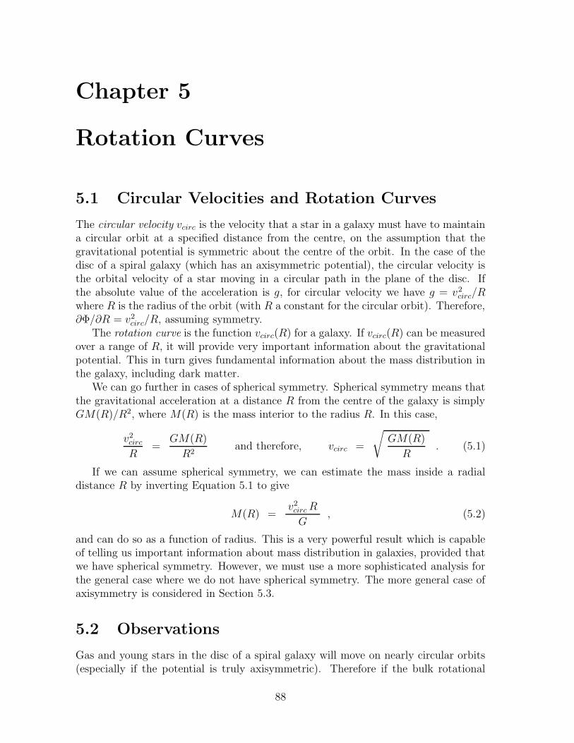
Chapter 5

Rotation Curves

5.1 Circular Velocities and Rotation Curves

The circular velocity vcirc is the velocity that a star in a galaxy must have to maintaina circular orbit at a specified distance from the centre, on the assumption that thegravitational potential is symmetric about the centre of the orbit. In the case of thedisc of a spiral galaxy (which has an axisymmetric potential), the circular velocity isthe orbital velocity of a star moving in a circular path in the plane of the disc. Ifthe absolute value of the acceleration is g, for circular velocity we have g = v2

circ/Rwhere R is the radius of the orbit (with R a constant for the circular orbit). Therefore,∂Φ/∂R = v2

circ/R, assuming symmetry.The rotation curve is the function vcirc(R) for a galaxy. If vcirc(R) can be measured

over a range of R, it will provide very important information about the gravitationalpotential. This in turn gives fundamental information about the mass distribution inthe galaxy, including dark matter.

We can go further in cases of spherical symmetry. Spherical symmetry means thatthe gravitational acceleration at a distance R from the centre of the galaxy is simplyGM(R)/R2, where M(R) is the mass interior to the radius R. In this case,

v2circ

R=

GM(R)

R2and therefore, vcirc =

√

GM(R)

R. (5.1)

If we can assume spherical symmetry, we can estimate the mass inside a radialdistance R by inverting Equation 5.1 to give

M(R) =v2

circR

G, (5.2)

and can do so as a function of radius. This is a very powerful result which is capableof telling us important information about mass distribution in galaxies, provided thatwe have spherical symmetry. However, we must use a more sophisticated analysis forthe general case where we do not have spherical symmetry. The more general case ofaxisymmetry is considered in Section 5.3.

5.2 Observations

Gas and young stars in the disc of a spiral galaxy will move on nearly circular orbits(especially if the potential is truly axisymmetric). Therefore if the bulk rotational

88

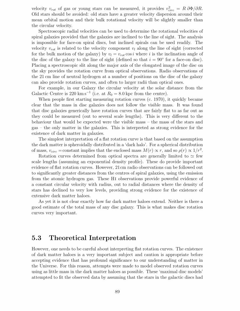
velocity vrot of gas or young stars can be measured, it provides v2circ = R ∂Φ/∂R.

Old stars should be avoided: old stars have a greater velocity dispersion around theirmean orbital motion and their bulk rotational velocity will be slightly smaller thanthe circular velocity.

Spectroscopic radial velocities can be used to determine the rotational velocities ofspiral galaxies provided that the galaxies are inclined to the line of sight. The analysisis impossible for face-on spiral discs, but inclined spirals can be used readily. Thevelocity vrot is related to the velocity component vl along the line of sight (correctedfor the bulk motion of the galaxy) by vl = vrot cos i where i is the inclination angle ofthe disc of the galaxy to the line of sight (defined so that i = 90◦ for a face-on disc).Placing a spectroscopic slit along the major axis of the elongated image of the disc onthe sky provides the rotation curve from optical observations. Radio observations ofthe 21 cm line of neutral hydrogen at a number of positions on the disc of the galaxycan also provide rotation curves, and often to larger radii than optical ones.

For example, in our Galaxy the circular velocity at the solar distance from theGalactic Centre is 220 km s−1 (i.e. at R0 = 8.0 kpc from the centre).

When people first starting measuring rotation curves (c. 1970), it quickly becameclear that the mass in disc galaxies does not follow the visible mass. It was foundthat disc galaxies generically have rotation curves that are fairly flat to as far out asthey could be measured (out to several scale lengths). This is very different to thebehaviour that would be expected were the visible mass – the mass of the stars andgas – the only matter in the galaxies. This is interpreted as strong evidence for theexistence of dark matter in galaxies.

The simplest interpretation of a flat rotation curve is that based on the assumptionthe dark matter is spheroidally distributed in a ‘dark halo’. For a spherical distributionof mass, vcirc =constant implies that the enclosed mass M(r) ∝ r, and so ρ(r) ∝ 1/r2.

Rotation curves determined from optical spectra are generally limited to ' fewscale lengths (assuming an exponential density profile). These do provide importantevidence of flat rotation curves. However, 21cm radio observations can be followed outto significantly greater distances from the centres of spiral galaxies, using the emissionfrom the atomic hydrogen gas. These H I observations provide powerful evidence ofa constant circular velocity with radius, out to radial distances where the density ofstars has declined to very low levels, providing strong evidence for the existence ofextensive dark matter haloes.

As yet it is not clear exactly how far dark matter haloes extend. Neither is there agood estimate of the total mass of any disc galaxy. This is what makes disc rotationcurves very important.

5.3 Theoretical Interpretation

However, one needs to be careful about interpreting flat rotation curves. The existenceof dark matter haloes is a very important subject and caution is appropriate beforeaccepting evidence that has profound significance to our understanding of matter inthe Universe. For this reason, attempts were made to model observed rotation curvesusing as little mass in the dark matter haloes as possible. These ‘maximal disc models’attempted to fit the observed data by assuming that the stars in the galactic discs had

89

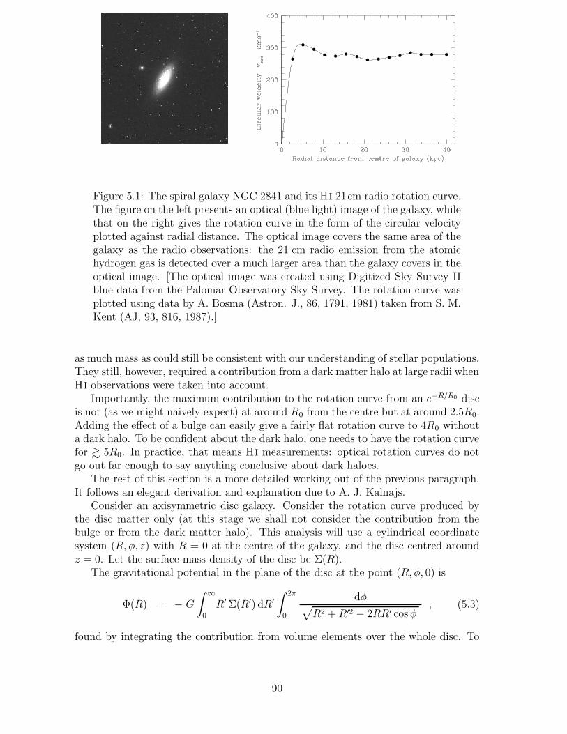
Figure 5.1: The spiral galaxy NGC 2841 and its H I 21cm radio rotation curve.The figure on the left presents an optical (blue light) image of the galaxy, whilethat on the right gives the rotation curve in the form of the circular velocityplotted against radial distance. The optical image covers the same area of thegalaxy as the radio observations: the 21 cm radio emission from the atomichydrogen gas is detected over a much larger area than the galaxy covers in theoptical image. [The optical image was created using Digitized Sky Survey IIblue data from the Palomar Observatory Sky Survey. The rotation curve wasplotted using data by A. Bosma (Astron. J., 86, 1791, 1981) taken from S. M.Kent (AJ, 93, 816, 1987).]

as much mass as could still be consistent with our understanding of stellar populations.They still, however, required a contribution from a dark matter halo at large radii whenH I observations were taken into account.

Importantly, the maximum contribution to the rotation curve from an e−R/R0 discis not (as we might naively expect) at around R0 from the centre but at around 2.5R0.Adding the effect of a bulge can easily give a fairly flat rotation curve to 4R0 withouta dark halo. To be confident about the dark halo, one needs to have the rotation curvefor & 5R0. In practice, that means H I measurements: optical rotation curves do notgo out far enough to say anything conclusive about dark haloes.

The rest of this section is a more detailed working out of the previous paragraph.It follows an elegant derivation and explanation due to A. J. Kalnajs.

Consider an axisymmetric disc galaxy. Consider the rotation curve produced bythe disc matter only (at this stage we shall not consider the contribution from thebulge or from the dark matter halo). This analysis will use a cylindrical coordinatesystem (R, φ, z) with R = 0 at the centre of the galaxy, and the disc centred aroundz = 0. Let the surface mass density of the disc be Σ(R).

The gravitational potential in the plane of the disc at the point (R, φ, 0) is

Φ(R) = − G

∫ ∞

0

R′ Σ(R′) dR′

∫ 2π

0

dφ√

R2 +R′2 − 2RR′ cosφ, (5.3)

found by integrating the contribution from volume elements over the whole disc. To

90

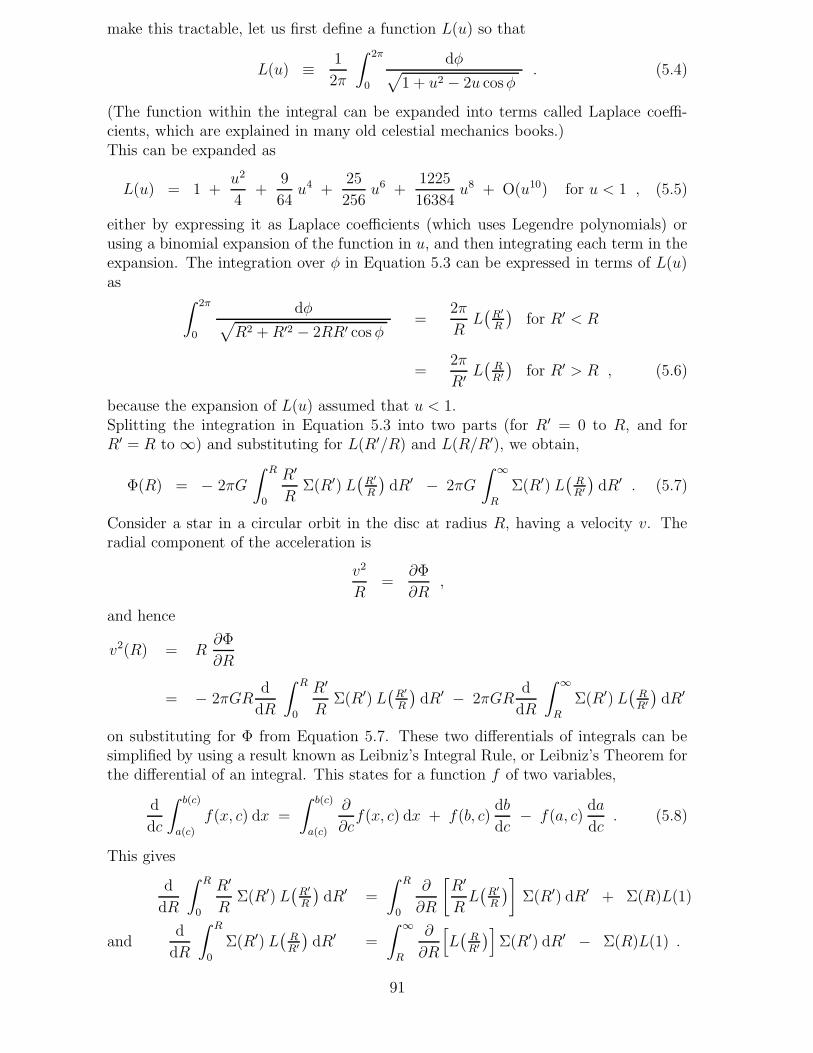
make this tractable, let us first define a function L(u) so that

L(u) ≡ 1

2π

∫ 2π

0

dφ√

1 + u2 − 2u cosφ. (5.4)

(The function within the integral can be expanded into terms called Laplace coeffi-cients, which are explained in many old celestial mechanics books.)This can be expanded as

L(u) = 1 +u2

4+

9

64u4 +

25

256u6 +

1225

16384u8 + O(u10) for u < 1 , (5.5)

either by expressing it as Laplace coefficients (which uses Legendre polynomials) orusing a binomial expansion of the function in u, and then integrating each term in theexpansion. The integration over φ in Equation 5.3 can be expressed in terms of L(u)as

∫ 2π

0

dφ√

R2 +R′2 − 2RR′ cos φ=

2π

RL(

R′

R

)

for R′ < R

=2π

R′L(

RR′

)

for R′ > R , (5.6)

because the expansion of L(u) assumed that u < 1.Splitting the integration in Equation 5.3 into two parts (for R′ = 0 to R, and forR′ = R to ∞) and substituting for L(R′/R) and L(R/R′), we obtain,

Φ(R) = − 2πG

∫ R

0

R′

RΣ(R′) L

(

R′

R

)

dR′ − 2πG

∫ ∞

R

Σ(R′) L(

RR′

)

dR′ . (5.7)

Consider a star in a circular orbit in the disc at radius R, having a velocity v. Theradial component of the acceleration is

v2

R=

∂Φ

∂R,

and hence

v2(R) = R∂Φ

∂R

= − 2πGRd

dR

∫ R

0

R′

RΣ(R′) L

(

R′

R

)

dR′ − 2πGRd

dR

∫ ∞

R

Σ(R′) L(

RR′

)

dR′

on substituting for Φ from Equation 5.7. These two differentials of integrals can besimplified by using a result known as Leibniz’s Integral Rule, or Leibniz’s Theorem forthe differential of an integral. This states for a function f of two variables,

d

dc

∫ b(c)

a(c)

f(x, c) dx =

∫ b(c)

a(c)

∂

∂cf(x, c) dx + f(b, c)

db

dc− f(a, c)

da

dc. (5.8)

This gives

d

dR

∫ R

0

R′

RΣ(R′) L

(

R′

R

)

dR′ =

∫ R

0

∂

∂R

[

R′

RL(

R′

R

)

]

Σ(R′) dR′ + Σ(R)L(1)

andd

dR

∫ R

0

Σ(R′) L(

RR′

)

dR′ =

∫ ∞

R

∂

∂R

[

L(

RR′

)

]

Σ(R′) dR′ − Σ(R)L(1) .

91

Therefore we get

v2(R) = − 2πGR

∫ R

0

d

dR

(

R′

RL(

R′

R

)

)

Σ(R′) dR′ − 2πGR

∫ ∞

R

Σ(R′)d

dRL(

RR′

)

dR′

But,

d

dR

(

R′

RL(

R′

R

)

)

= − R′

R2L(

R′

R

)

+R′

R

d

dRL(

R′

R

)

from the product rule

= − R′

R2L(

R′

R

)

+R′

R

dL(

R′

R

)

d(R′/R)

d(R′/R)

dRfrom the chain rule

= − R′

R2L(

R′

R

)

− R′2

R3L′(

R′

R

)

writing L′(u) ≡ dL(u)du

.

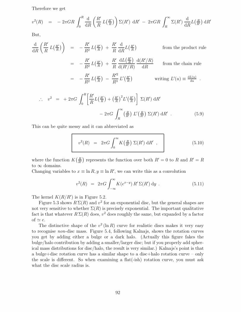
∴ v2 = + 2πG

∫ R

0

[

R′

RL(

R′

R

)

+(

R′

R

)2L′(

R′

R

)

]

Σ(R′) dR′

− 2πG

∫ ∞

R

(

RR′

)

L′(

RR′

)

Σ(R′) dR′ . (5.9)

This can be quite messy and it can abbreviated as

v2(R) = 2πG

∫ ∞

0

K(

RR′

)

Σ(R′) dR′ , (5.10)

where the function K(

RR′

)

represents the function over both R′ = 0 to R and R′ = Rto ∞ domains.Changing variables to x ≡ lnR, y ≡ lnR′, we can write this as a convolution

v2(R) = 2πG

∫ ∞

−∞

K(ex−y)R′ Σ(R′) dy . (5.11)

The kernel K(R/R′) is in Figure 5.2.Figure 5.3 shows RΣ(R) and v2 for an exponential disc, but the general shapes are

not very sensitive to whether Σ(R) is precisely exponential. The important qualitativefact is that whatever RΣ(R) does, v2 does roughly the same, but expanded by a factorof ' e.

The distinctive shape of the v2 (lnR) curve for realistic discs makes it very easyto recognise non-disc mass. Figure 5.4, following Kalnajs, shows the rotation curvesyou get by adding either a bulge or a dark halo. (Actually this figure fakes thebulge/halo contribution by adding a smaller/larger disc; but if you properly add spher-ical mass distributions for disc/halo, the result is very similar.) Kalnajs’s point is thata bulge+disc rotation curve has a similar shape to a disc+halo rotation curve – onlythe scale is different. So when examining a flat(-ish) rotation curve, you must askwhat the disc scale radius is.

92

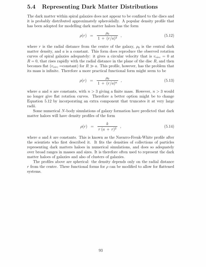
5.4 Representing Dark Matter Distributions

The dark matter within spiral galaxies does not appear to be confined to the discs andit is probably distributed approximately spheroidally. A popular density profile thathas been adopted for modelling dark matter haloes has the form

ρ(r) =ρ0

1 + (r/a)2, (5.12)

where r is the radial distance from the centre of the galaxy, ρ0 is the central darkmatter density, and a is a constant. This form does reproduce the observed rotationcurves of spiral galaxies adequately: it gives a circular velocity that is vcirc = 0 atR = 0, that rises rapidly with the radial distance in the plane of the disc R, and thenbecomes flat (vcirc =constant) for R � a. This profile, however, has the problem thatits mass is infinite. Therefore a more practical functional form might seem to be

ρ(r) =ρ0

1 + (r/a)n, (5.13)

where a and n are constants, with n > 3 giving a finite mass. However, n > 3 wouldno longer give flat rotation curves. Therefore a better option might be to changeEquation 5.12 by incorporating an extra component that truncates it at very largeradii.

Some numerical N -body simulations of galaxy formation have predicted that darkmatter haloes will have density profiles of the form

ρ(r) =k

r (a + r)2, (5.14)

where a and k are constants. This is known as the Navarro-Frenk-White profile afterthe scientists who first described it. It fits the densities of collections of particlesrepresenting dark matters haloes in numerical simulations, and does so adequatelyover broad ranges in masses and sizes. It is therefore often used to represent the darkmatter haloes of galaxies and also of clusters of galaxies.

The profiles above are spherical: the density depends only on the radial distancer from the centre. These functional forms for ρ can be modified to allow for flattenedsystems.

93

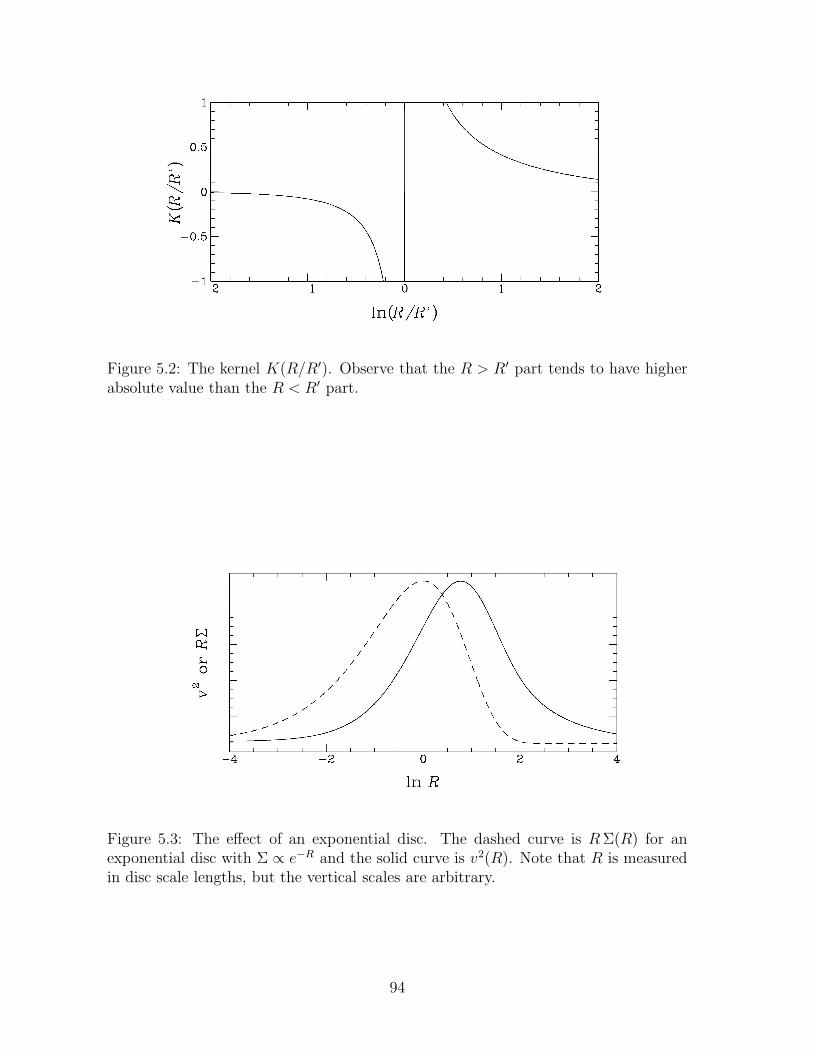
Figure 5.2: The kernel K(R/R′). Observe that the R > R′ part tends to have higherabsolute value than the R < R′ part.

Figure 5.3: The effect of an exponential disc. The dashed curve is RΣ(R) for anexponential disc with Σ ∝ e−R and the solid curve is v2(R). Note that R is measuredin disc scale lengths, but the vertical scales are arbitrary.

94

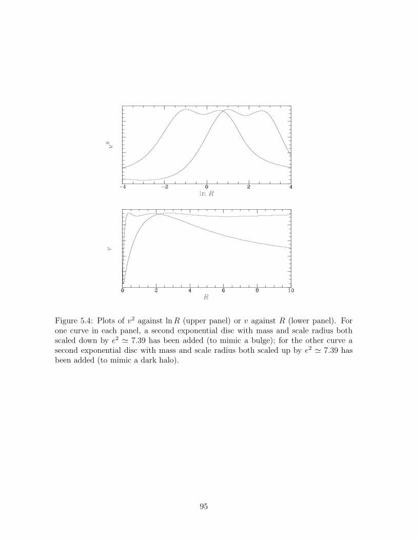
Figure 5.4: Plots of v2 against lnR (upper panel) or v against R (lower panel). Forone curve in each panel, a second exponential disc with mass and scale radius bothscaled down by e2 ' 7.39 has been added (to mimic a bulge); for the other curve asecond exponential disc with mass and scale radius both scaled up by e2 ' 7.39 hasbeen added (to mimic a dark halo).

95