Logistic Regression

1

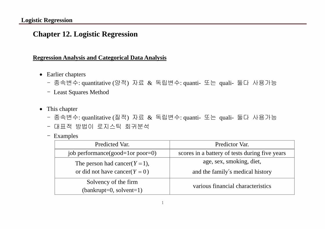
Chapter 12. Logistic Regression

Regression Analysis and Categorical Data Analysis

Earlier chapters - 종속변수: quantitative (양적) 자료 & 독립변수: quanti- 또는 quali- 둘다 사용가능 - Least Squares Method

This chapter

- 종속변수: quanlitative (질적) 자료 & 독립변수: quanti- 또는 quali- 둘다 사용가능 - 대표적 방법이 로지스틱 회귀분석 - Examples

Predicted Var. Predictor Var. job performance(good=1or poor=0) scores in a battery of tests during five years

The person had cancer( 1Y ), or did not have cancer( 0Y )

age, sex, smoking, diet,

and the family’s medical history

Solvency of the firm (bankrupt=0, solvent=1)

various financial characteristics

Logistic Regression

2

Modeling Qualitative Data

• Rather than predicting these two values of the binary response variable, we try to model the

probabilities that the response takes one of these two values.

• Let denote the probability that 1Y when X x .

• If we use the standard linear model, we cannot model probability;

0 1Pr( 1 )Y X x x .

- LHS lies between 0 and 1 while RHS is unbounded.

- 참고: weighted least squares in logistic regression complicated

• Logistic model: 0 1

0 1Pr( 1 )

1

x

x

eY X xe

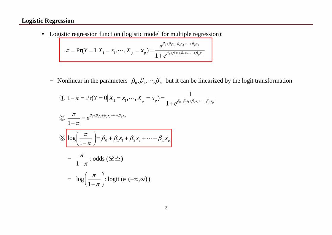
Logistic Regression

3

Logistic regression function (logistic model for multiple regression):

1 1Pr( 1 , , )p pY X x X x 0 1 1 2 2

0 1 1 2 21

p p

p p

x x x

x x xe

e

- Nonlinear in the parameters 0 1, , , p but it can be linearized by the logit transformation

① 0 1 1 2 21 1

11 Pr( 0 , , )1 p pp p x x xY X x X x

e

② 0 1 1 2 2

1p px x xe

③ 0 1 1 2 2log1 p px x x

- 1

: odds (오즈)

- log1

: logit ( ( , ) )

Logistic Regression

4

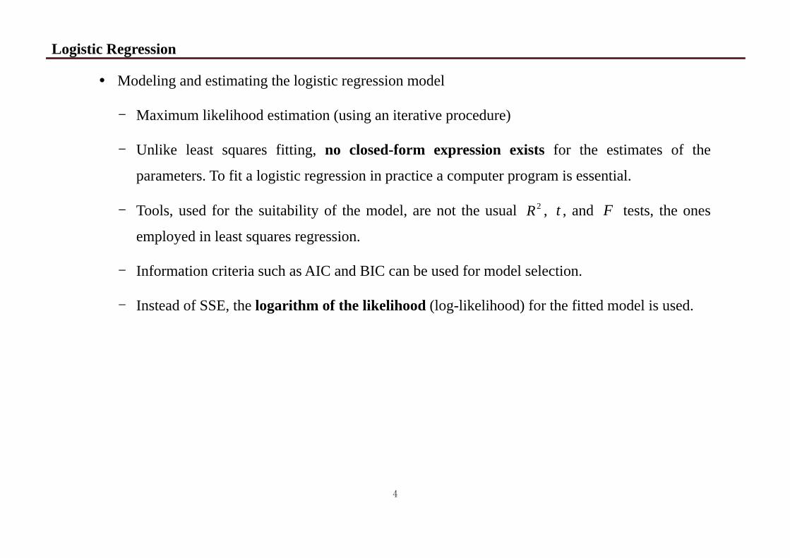
Modeling and estimating the logistic regression model

- Maximum likelihood estimation (using an iterative procedure)

- Unlike least squares fitting, no closed-form expression exists for the estimates of the

parameters. To fit a logistic regression in practice a computer program is essential.

- Tools, used for the suitability of the model, are not the usual 2R , t , and F tests, the ones

employed in least squares regression.

- Information criteria such as AIC and BIC can be used for model selection.

- Instead of SSE, the logarithm of the likelihood (log-likelihood) for the fitted model is used.

Logistic Regression

5

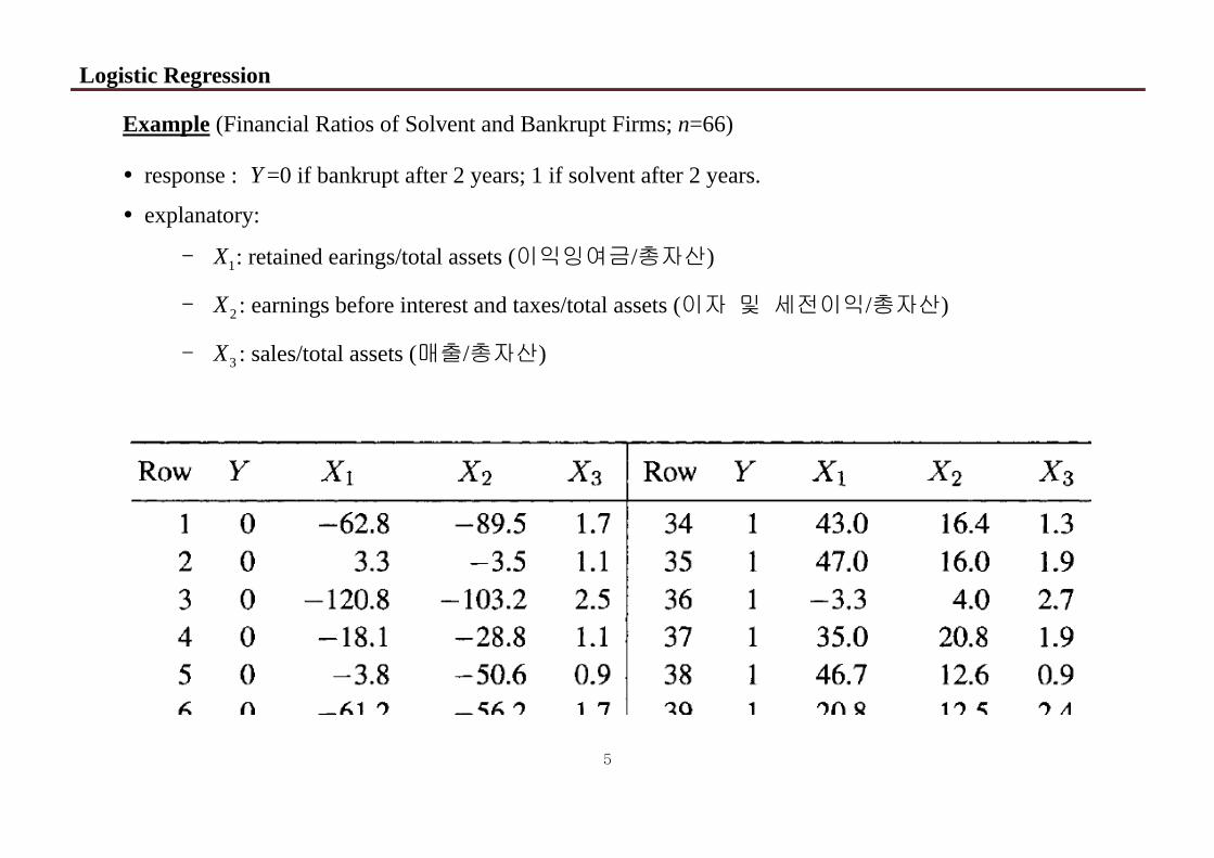
Example (Financial Ratios of Solvent and Bankrupt Firms; n=66)

response : Y =0 if bankrupt after 2 years; 1 if solvent after 2 years.

explanatory:

- 1X : retained earings/total assets (이익잉여금/총자산)

- 2X : earnings before interest and taxes/total assets (이자 및 세전이익/총자산)

- 3X : sales/total assets (매출/총자산)

Logistic Regression

6

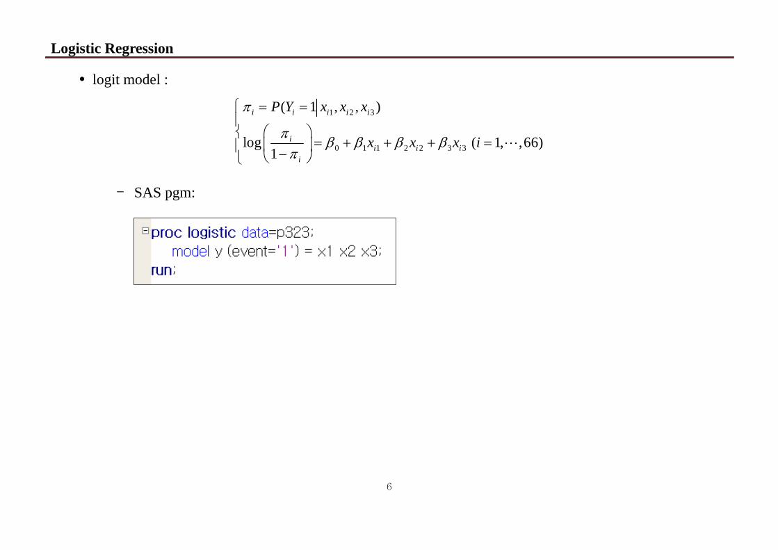
logit model :

1 2 3

0 1 1 2 2 3 3

( 1 , , )

log ( 1, ,66)1

i i i i i

ii i i

i

P Y x x x

x x x i

- SAS pgm:

Logistic Regression

7

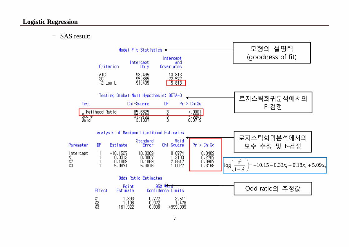
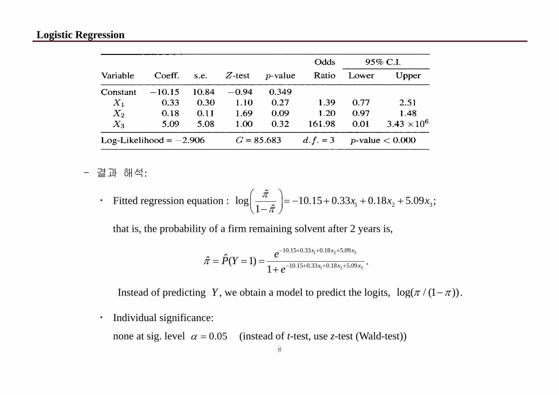
- SAS result:

모형의 설명력(goodness of fit)

로지스틱회귀분석에서의 F-검정

로지스틱회귀분석에서의 모수 추정 및 t-검정

Odd ratio의 추정값

1 2 3ˆlog 10.15 0.33 0.18 5.09

ˆ1x x x

Logistic Regression

8

- 결과 해석:

Fitted regression equation : 1 2 3ˆlog 10.15 0.33 0.18 5.09

ˆ1x x x

;

that is, the probability of a firm remaining solvent after 2 years is,

1 2 3

1 2 3

10.15 0.33 0.18 5.09

10.15 0.33 0.18 5.09ˆˆ ( 1)

1

x x x

x x xeP Y

e

.

Instead of predicting Y , we obtain a model to predict the logits, log( / (1 )) .

Individual significance:

none at sig. level 0.05 (instead of t-test, use z-test (Wald-test))

Logistic Regression

9

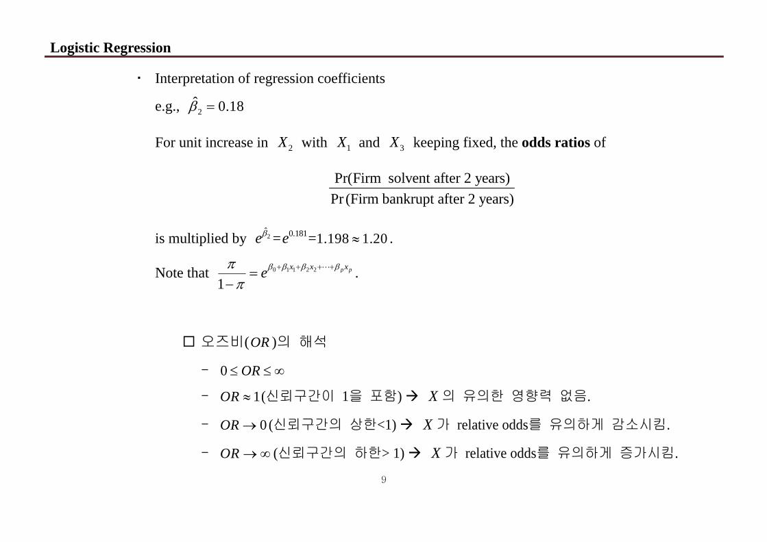
Interpretation of regression coefficients

e.g., 2ˆ 0.18

For unit increase in 2X with 1X and 3X keeping fixed, the odds ratios of

Pr(Firm solvent after 2 years)Pr (Firm bankrupt after 2 years)

is multiplied by 2ˆe = 0.181e =1.198 1.20 .

Note that 0 1 1 2 2

1p px x xe

.

오즈비(OR )의 해석

- 0 OR

- 1OR (신뢰구간이 1을 포함) X 의 유의한 영향력 없음.

- 0OR (신뢰구간의 상한<1) X 가 relative odds를 유의하게 감소시킴.

- OR (신뢰구간의 하한> 1) X 가 relative odds를 유의하게 증가시킴.

Logistic Regression

10

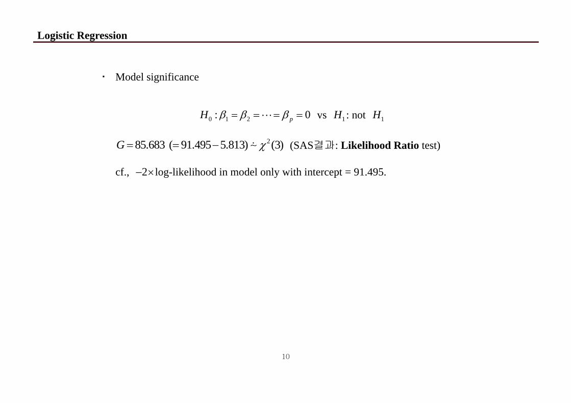
Model significance

0 1 2: 0pH vs 1H : not 1H

285.683 ( 91.495 5.813) (3)G (SAS결과: Likelihood Ratio test)

cf., 2 log-likelihood in model only with intercept = 91.495.

Logistic Regression

11

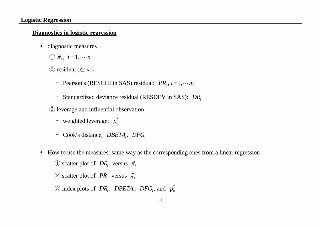
Diagnostics in logistic regression

diagnostic measures

① ˆi , 1, ,i n

② residual (잔차)

- Pearson’s (RESCHI in SAS) residual: , 1, ,iPR i n

- Standardized deviance residual (RESDEV in SAS): iDR

③ leverage and influential observation

- weighted leverage: *iip

- Cook’s distance, iDBETA , iDFG

How to use the measures: same way as the corresponding ones from a linear regression

① scatter plot of iDR versus ˆi

② scatter plot of iPR versus ˆi

③ index plots of iDR , iDBETA , iDFG , and *iip

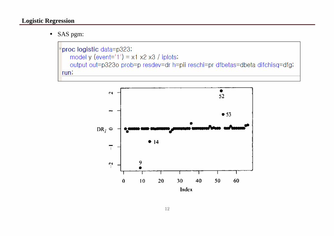
Logistic Regression

12

SAS pgm:

Logistic Regression

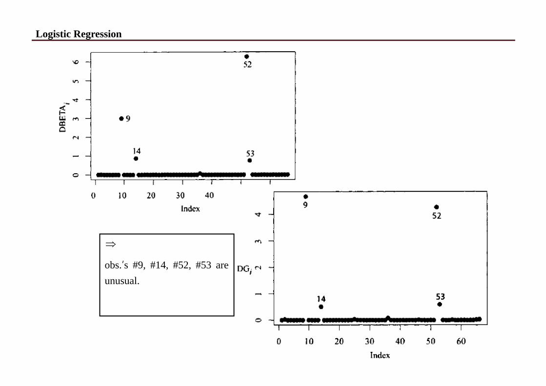
13

obs.’s #9, #14, #52, #53 are unusual.

Logistic Regression

14

Determination of Variables to Retain (§12.6)

• Model is significant but none of individual predictors are significant. Do we need all three variables? (Also, you can check multicollinearity)

• Instead of looking at the reduction in the error sum of squares (SSE), we look at the change in the (log) likelihood for the two fitted models in logistic regression.

• To see whether the q additional variables are significant, we look

2 ( ) ( )G L p L p q

- ( )L p : log likelihood for a model with p variables and constant - ( )L p q : log likelihood for a model with p q variables and constant

- 2~ ( )G q under the null 0 1 2: 0p p p qH

- A large value of the test statistic would call for the retention of the q variables in the model.

- The test is valid when n is large.

• With a large number of explanatory variables the side-by-side boxplots provide a quick screening procedure.

Logistic Regression

15

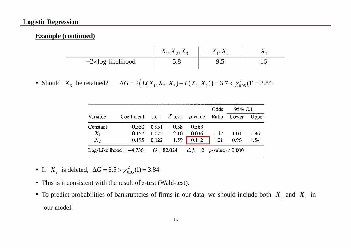
Example (continued)

1 2 3, ,X X X 1 2,X X 1X 2 log-likelihood 5.8 9.5 16

Should 3X be retained? 2

1 2 3 1 2 0.052 ( , , ) ( , ) 3.7 (1) 3.84G L X X X L X X

If 2X is deleted, 20.056.5 (1) 3.84G

This is inconsistent with the result of z-test (Wald-test).

To predict probabilities of bankruptcies of firms in our data, we should include both 1X and 2X in

our model.

Logistic Regression

16

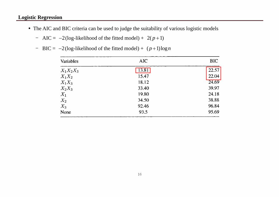
The AIC and BIC criteria can be used to judge the suitability of various logistic models

- AIC = 2 (log-likelihood of the fitted model) + 2( 1)p

- BIC = 2 (log-likelihood of the fitted model) + ( 1)logp n

Logistic Regression

17

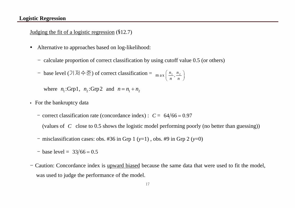
Judging the fit of a logistic regression (§12.7)

Alternative to approaches based on log-likelihood:

- calculate proportion of correct classification by using cutoff value 0.5 (or others)

- base level (기저수준) of correct classification = 1 2m a x ,n nn n

where 1:Grp1n , 2 :Grp2n and 1 2n n n

For the bankruptcy data

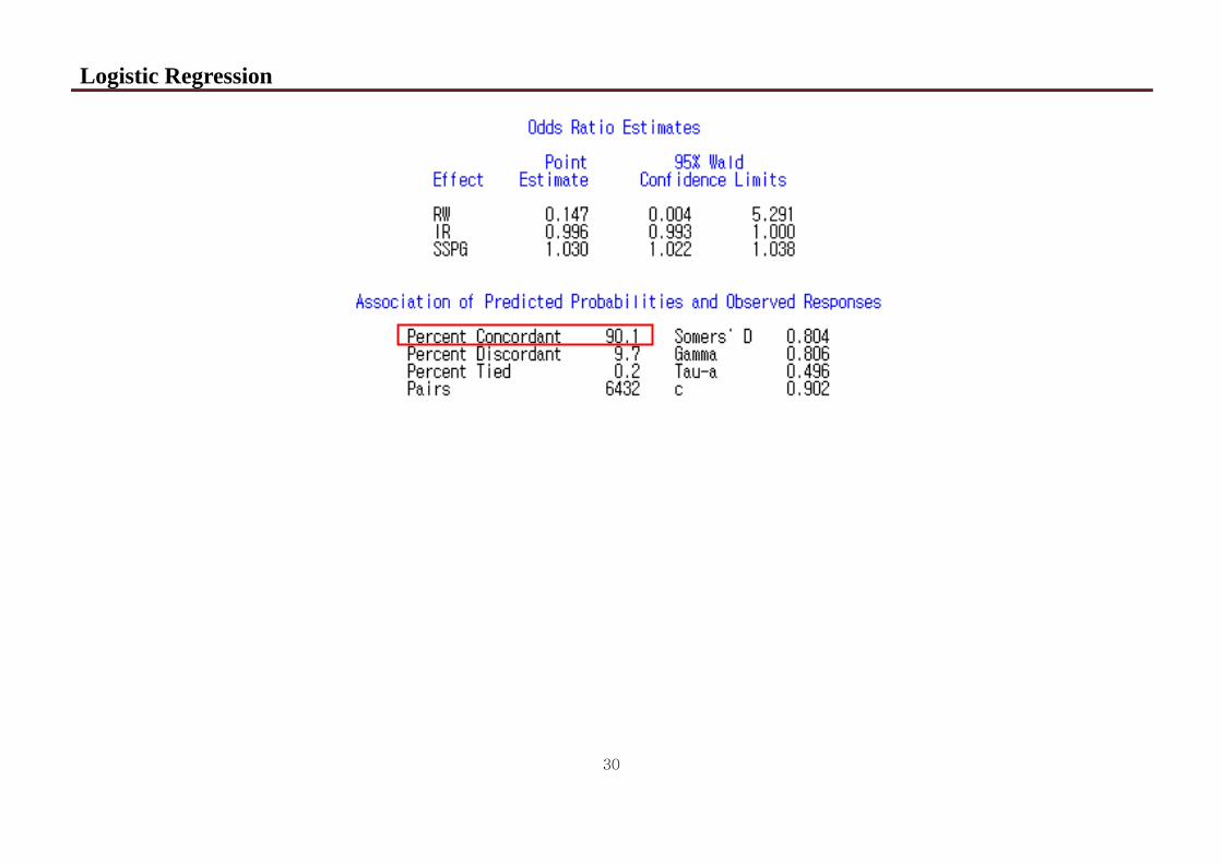
- correct classification rate (concordance index) : C = 64 66 0.97

(values of C close to 0.5 shows the logistic model performing poorly (no better than guessing))

- misclassification cases: obs. #36 in Grp 1 (y=1) , obs. #9 in Grp 2 (y=0)

- base level = 33 66 0.5

- Caution: Concordance index is upward biased because the same data that were used to fit the model,

was used to judge the performance of the model.

Logistic Regression

18

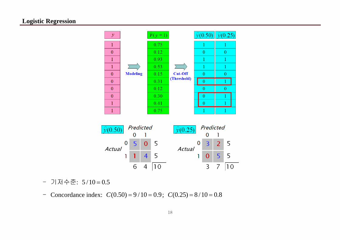
- 기저수준: 5 /10 0.5

- Concordance index: (0.50) 9 /10 0.9C ; (0.25) 8 /10 0.8C

Logistic Regression

19

Multinomial Logit Model (다항 로짓 모형)

Logistic reg. model extended to situations where the response variable assumes more than two values

- Case 1: multinomial (polytomous) logistic regression (다항 로지스틱 회귀)

response categories are not ordered ;

e.g., choice of mode of transportation to work: private automobile, car pool, public transport,

bicycle, or walking

- Case 2: proportional odds model (비례 오즈 모형)

response categories are ordered

e.g., an opinion survey (strongly agree, agree, no opinion, disagree, and strongly disagree)

and a clinical trial with responses to a treatment (improved, no change, worse)

Logistic Regression

20

Multinomial Logistic Regression

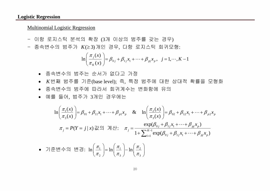
- 이항 로지스틱 분석의 확장 (3개 이상의 범주를 갖는 경우) - 종속변수의 범주가 ( 3)K 개인 경우, 다항 로지스틱 회귀모형:

0 1 1

( )ln

( )j

j j pj pK

xx x

x

, 1, , 1j K

종속변수의 범주는 순서가 없다고 가정 K번째 범주를 기준(base level); 즉, 특정 범주에 대한 상대적 확률을 모형화 종속변수의 범주에 따라서 회귀계수는 변화함에 유의 예를 들어, 범주가 3개인 경우에는

101 11 1 1

3

( )ln( ) p px x xx

& 202 12 1 2

3

( )ln( ) p px x xx

( | )j P Y j x 값의 계산: 0 1 11

0 1 11

exp( )

1 exp( )j j pj p

j Kj j pj pi

x x

x x

기준변수의 변경: 1 1 2

2 3 3

ln ln ln

Logistic Regression

21

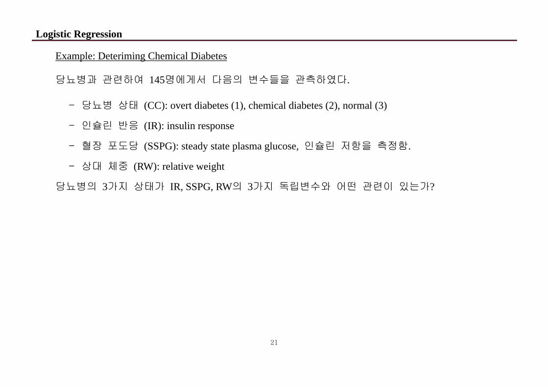
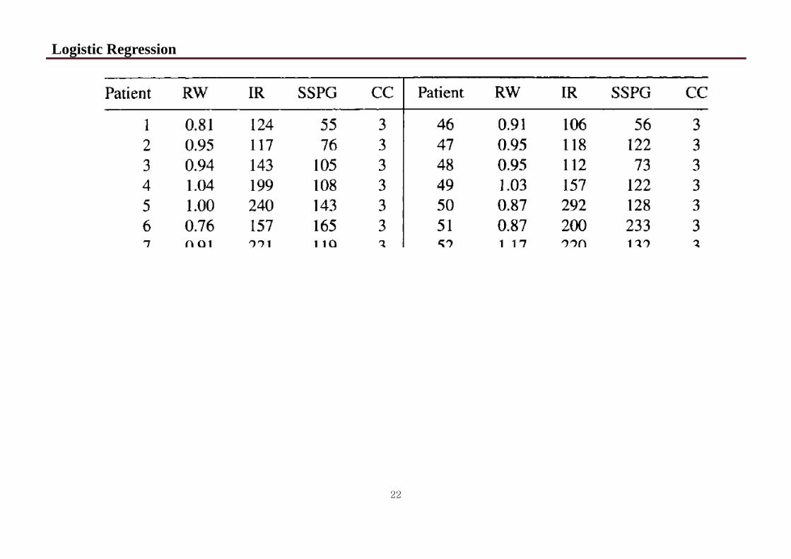
Example: Deteriming Chemical Diabetes

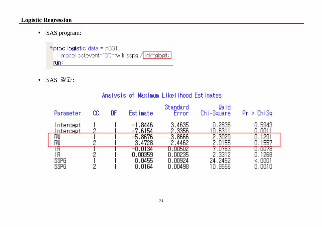
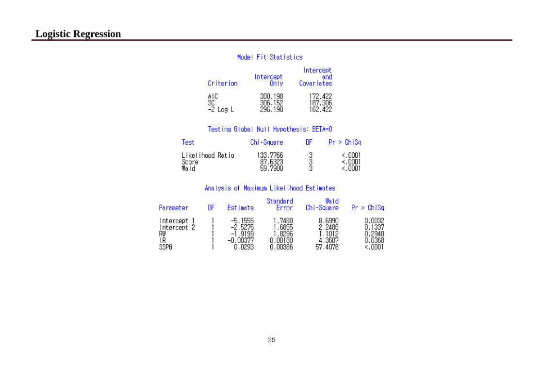
당뇨병과 관련하여 145명에게서 다음의 변수들을 관측하였다.

- 당뇨병 상태 (CC): overt diabetes (1), chemical diabetes (2), normal (3)

- 인슐린 반응 (IR): insulin response

- 혈장 포도당 (SSPG): steady state plasma glucose, 인슐린 저항을 측정함.

- 상대 체중 (RW): relative weight

당뇨병의 3가지 상태가 IR, SSPG, RW의 3가지 독립변수와 어떤 관련이 있는가?

Logistic Regression

22

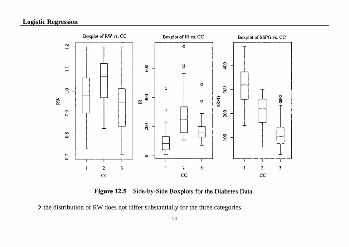
Logistic Regression

23

the distribution of RW does not differ substantially for the three categories.

Logistic Regression

24

SAS program:

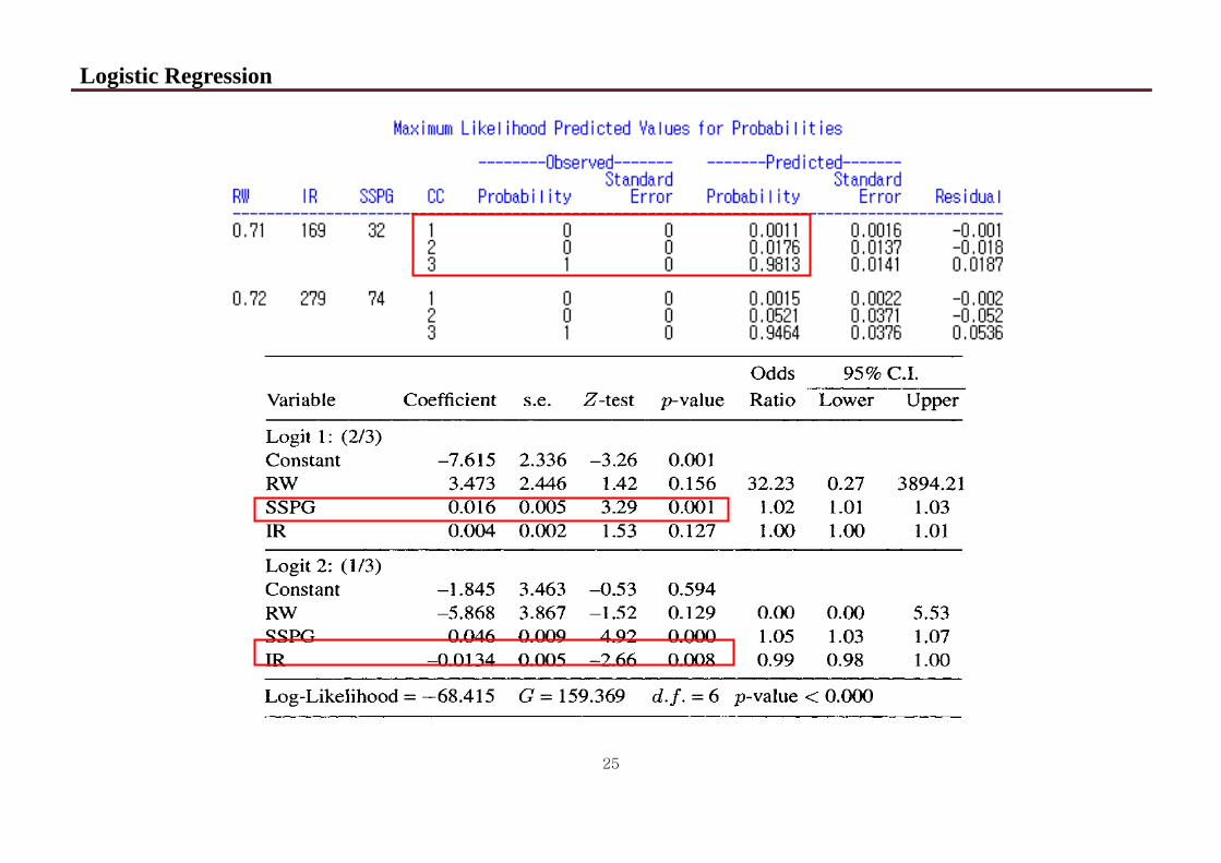
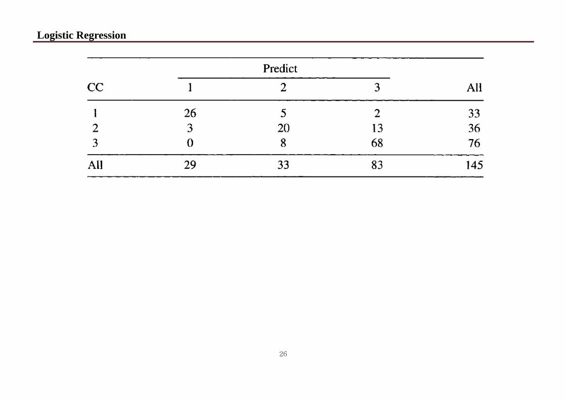
SAS 결과:

Logistic Regression

25

Logistic Regression

26

Logistic Regression

27

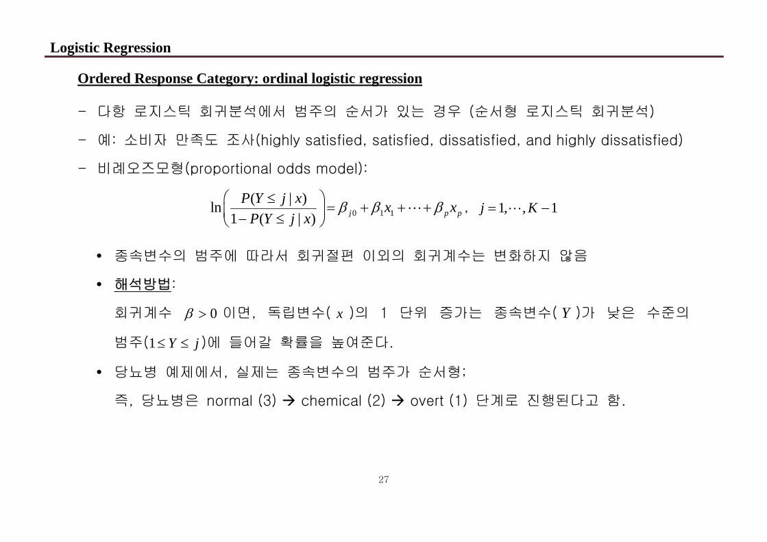
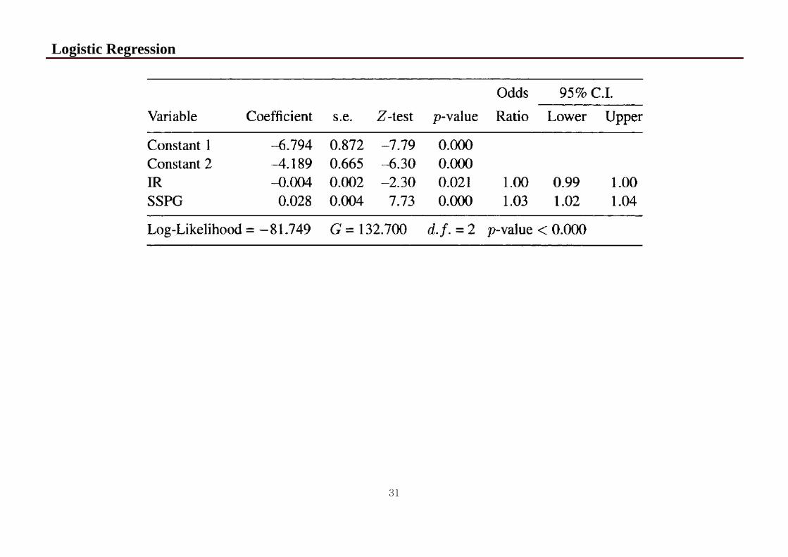
Ordered Response Category: ordinal logistic regression

- 다항 로지스틱 회귀분석에서 범주의 순서가 있는 경우 (순서형 로지스틱 회귀분석)

- 예: 소비자 만족도 조사(highly satisfied, satisfied, dissatisfied, and highly dissatisfied)

- 비례오즈모형(proportional odds model):

0 1 1( | )ln

1 ( | ) j p pP Y j x x x

P Y j x

, 1, , 1j K

종속변수의 범주에 따라서 회귀절편 이외의 회귀계수는 변화하지 않음

해석방법:

회귀계수 0 이면, 독립변수( x )의 1 단위 증가는 종속변수( Y )가 낮은 수준의

범주(1 Y j )에 들어갈 확률을 높여준다.

당뇨병 예제에서, 실제는 종속변수의 범주가 순서형;

즉, 당뇨병은 normal (3) chemical (2) overt (1) 단계로 진행된다고 함.

Logistic Regression

28

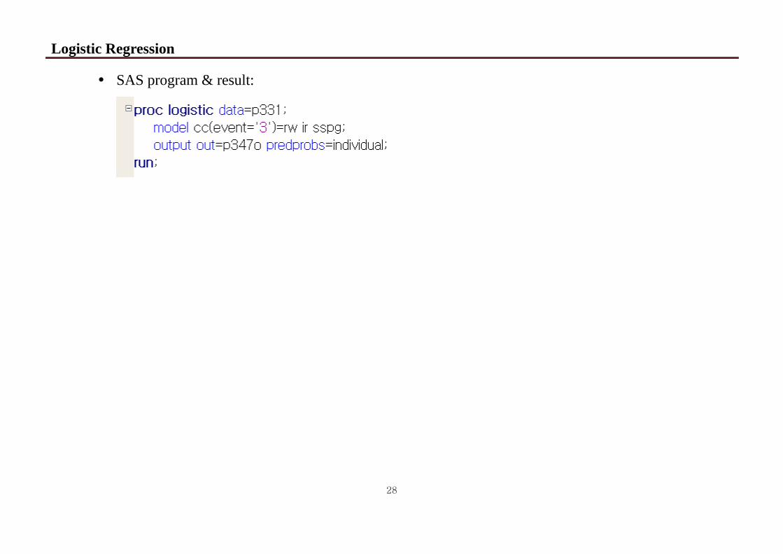
SAS program & result:

Logistic Regression

29

Logistic Regression

30

Logistic Regression

31