Chapter 2

A Quick Review of ProbabilityTheory

These notes are not intended to be a comprehensive introduction to the theory ofprobability. Instead, they constitute a brief introduction that should be sufficientto allow a student to understand the stochastic models they will encounter in laterchapters. These notes were heavily influenced by Sheldon Ross’s text [14], and TimoSeppalainen’s notes on probability theory that serve a similar purpose [15]. Anystudent who finds this material difficult should review an introductory probabilitybook such as Sheldon Ross’s A first course in probability [14], which is on reserve inthe Math library.

2.1 The Probability Space

Probability theory is used to model experiments (defined loosely) whose outcome cannot be predicted with certainty beforehand. For any such experiment, there is a triple(Ω,F , P ), called a probability space, where

• Ω is the sample space,

• F is a collection of events,

• P is a probability measure.

We will consider each in turn.

2.1.1 The sample space Ω

The sample space of an experiment is the set of all possible outcomes. Elements of Ωare called sample points and are often denoted by ω. Subsets of Ω are referred to asevents.

0Copyright c 2011 by David F. Anderson.

15

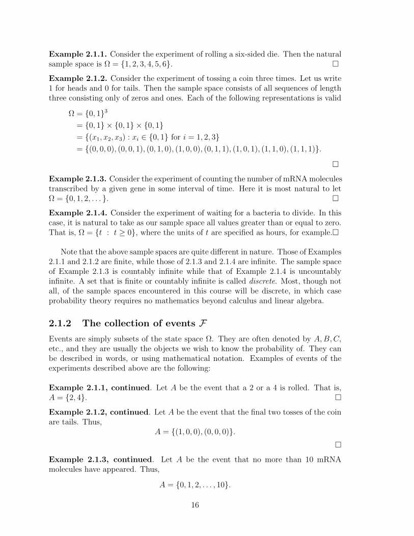
Example 2.1.1. Consider the experiment of rolling a six-sided die. Then the naturalsample space is Ω = 1, 2, 3, 4, 5, 6. Example 2.1.2. Consider the experiment of tossing a coin three times. Let us write1 for heads and 0 for tails. Then the sample space consists of all sequences of lengththree consisting only of zeros and ones. Each of the following representations is valid

Ω = 0, 13

= 0, 1× 0, 1× 0, 1= (x1, x2, x3) : xi ∈ 0, 1 for i = 1, 2, 3= (0, 0, 0), (0, 0, 1), (0, 1, 0), (1, 0, 0), (0, 1, 1), (1, 0, 1), (1, 1, 0), (1, 1, 1).

Example 2.1.3. Consider the experiment of counting the number of mRNAmoleculestranscribed by a given gene in some interval of time. Here it is most natural to letΩ = 0, 1, 2, . . . . Example 2.1.4. Consider the experiment of waiting for a bacteria to divide. In thiscase, it is natural to take as our sample space all values greater than or equal to zero.That is, Ω = t : t ≥ 0, where the units of t are specified as hours, for example.

Note that the above sample spaces are quite different in nature. Those of Examples2.1.1 and 2.1.2 are finite, while those of 2.1.3 and 2.1.4 are infinite. The sample spaceof Example 2.1.3 is countably infinite while that of Example 2.1.4 is uncountablyinfinite. A set that is finite or countably infinite is called discrete. Most, though notall, of the sample spaces encountered in this course will be discrete, in which caseprobability theory requires no mathematics beyond calculus and linear algebra.

2.1.2 The collection of events FEvents are simply subsets of the state space Ω. They are often denoted by A,B,C,

etc., and they are usually the objects we wish to know the probability of. They canbe described in words, or using mathematical notation. Examples of events of theexperiments described above are the following:

Example 2.1.1, continued. Let A be the event that a 2 or a 4 is rolled. That is,A = 2, 4. Example 2.1.2, continued. Let A be the event that the final two tosses of the coinare tails. Thus,

A = (1, 0, 0), (0, 0, 0).

Example 2.1.3, continued. Let A be the event that no more than 10 mRNAmolecules have appeared. Thus,

A = 0, 1, 2, . . . , 10.

16

Example 2.1.4, continued. Let A be the event that it took longer than 2 hoursfor the bacteria to divide. Then,

A = t : t > 2.

We will often have need to consider the unions and intersections of events. We

write A ∪ B for the union of A and B, and either A ∩ B or AB for the intersection.For discrete sample spaces, F will contain all subsets of Ω, and will play very

little role. This is the case for nearly all of the models in this course. When the statespace is more complicated, F is assumed to be a σ-algebra. That is, it satisfies thefollowing three axioms:

1. Ω ∈ F .

2. If A ∈ F , then Ac ∈ F , where Ac is the complement of A.

3. If A1, A2, . . . ,∈ F , then∞

i=1

Ai ∈ F .

2.1.3 The probability measure P

Definition 2.1.5. The real valued function P , with domain F , is a probability mea-sure if it satisfies the following three axioms

1. P (Ω) = 1.

2. If A ∈ F (or equivalently for discrete spaces if A ⊂ Ω), then P (A) ≥ 0.

3. If for a sequence of events A1, A2, . . . ,, we have that Ai ∩ Aj = ∅ for all i = j

(i.e. the sets are mutually exclusive) then

P

∞

i=1

Ai

=

∞

i=1

P (Ai).

The following is a listing of some of the basic properties of any probability measure,which are stated without proof.

Lemma 2.1.6. Let P (·) be a probability measure. Then

1. If A1, . . . , An is a finite sequence of mutually exclusive events, then

P

n

i=1

Ai

=

n

i=1

P (Ai).

2. P (Ac) = 1− P (A).

17

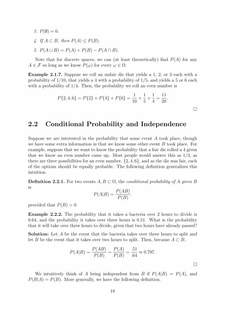
3. P (∅) = 0.

4. If A ⊂ B, then P (A) ≤ P (B).

5. P (A ∪ B) = P (A) + P (B)− P (A ∩ B).

Note that for discrete spaces, we can (at least theoretically) find P (A) for anyA ∈ F so long as we know P (ω) for every ω ∈ Ω.

Example 2.1.7. Suppose we roll an unfair die that yields a 1, 2, or 3 each with aprobability of 1/10, that yields a 4 with a probability of 1/5, and yields a 5 or 6 eachwith a probability of 1/4. Then, the probability we roll an even number is

P2, 4, 6 = P2+ P4+ P6 =1

10+

1

5+

1

4=

11

20.

2.2 Conditional Probability and Independence

Suppose we are interested in the probability that some event A took place, thoughwe have some extra information in that we know some other event B took place. Forexample, suppose that we want to know the probability that a fair die rolled a 4 giventhat we know an even number came up. Most people would answer this as 1/3, asthere are three possibilities for an even number, 2, 4, 6, and as the die was fair, eachof the options should be equally probable. The following definition generalizes thisintuition.

Definition 2.2.1. For two events A,B ⊂ Ω, the conditional probability of A given B

is

P (A|B) =P (AB)

P (B).

provided that P (B) > 0.

Example 2.2.2. The probability that it takes a bacteria over 2 hours to divide is0.64, and the probability it takes over three hours is 0.51. What is the probabilitythat it will take over three hours to divide, given that two hours have already passed?

Solution: Let A be the event that the bacteria takes over three hours to split andlet B be the event that it takes over two hours to split. Then, because A ⊂ B,

P (A|B) =P (AB)

P (B)=

P (A)

P (B)=

.51

.64≈ 0.797.

We intuitively think of A being independent from B if P (A|B) = P (A), andP (B|A) = P (B). More generally, we have the following definition.

18

Definition 2.2.3. The events A,B ∈ F are called independent if

P (AB) = P (A)P (B).

It is easy to check that the definition of independence implies both P (A|B) = P (A)and P (B|A) = P (B), and vice versa when P (A) > 0 and P (B) > 0. The concept ofindependence will play a key role in our study of Markov chains.

Theorem 2.2.4. Let Ω be a sample space with B ∈ F , and P (B) > 0. Then

(a) P (A | B) ≥ 0 for any event A ∈ F .

(b) P (Ω | B) = 1.

(c) If A1, A2, · · · ∈ F is a sequence of mutually exclusive events, then

P

∞

i=1

Ai | B

=∞

i=1

P (Ai|B).

Therefore, conditional probability measures are themselves probability measures,and we may write Q(·) = P (· | B).

By definition

P (A|B) =P (AB)

P (B), and P (B|A) = P (AB)

P (A).

Rearranging terms yields

P (AB) = P (A|B)P (B), and P (AB) = P (B|A)P (A).

This can be generalized further to the following.

Theorem 2.2.5. If P (A1A2 · · ·An) > 0, then

P (A1A2 · · ·An) = P (A1)P (A2 | A1)P (A3 | A1A2)P (A4 | A1A2A3) · · ·P (An | A1A2 · · ·An−1).

Definition 2.2.6. Let B1, . . . , Bn be a set of nonempty subsets of F . If the sets Bi

are mutually exclusive and

Bi = Ω, then the set B1, . . . , Bn is called a partitionof Ω.

Theorem 2.2.7 (Law of total probability). Let B1, . . . , Bn be a partition of Ω withP (Bi) > 0. Then for any A ∈ F

P (A) =n

i=1

P (A|Bi)P (Bi).

19

Theorem 2.2.8 (Bayes’ Theorem). For all events A,B ∈ F such that P (B) > 0 wehave

P (A|B) =P (B|A)P (A)

P (B).

This allows us to “turn conditional probabilities around.”

Proof. We have

P (A|B) =P (A ∩B)

P (B)=

P (B|A)P (A)

P (B)

2.3 Random Variables

Henceforth, we assume the existence of some probability space (Ω,F , P ). All randomvariables are assumed to be defined on this space in the following manner.

Definition 2.3.1. A random variable X is a real-valued function defined on thesample space Ω. That is, X : Ω → R.

If the range of X is finite or countably infinite, then X is said to be a discreterandom variable, whereas if the range is an interval of the real line (or some otheruncountably infinite set), then X is said to be a continuous random variable.

Example 2.3.2. Suppose we roll two die and take Ω = (i, j) | i, j ∈ 1, . . . , 6.We let X(i, j) = i + j be the discrete random variable giving the sum of the rolls.The range is 2, . . . , 12.

Example 2.3.3. Consider two bacteria, labeled 1 and 2. Let T1 and T2 denotethe times they will divide to give birth to daughter cells, respectively. Then, Ω =(T1, T2) | T1, T2 ≥ 0. Let X be the continuous random variable giving the time ofthe first division: X(T1, T2) = minT1, T2. The range of X is t ∈ R≥0.

Notation: As is traditional, we will write X ∈ I as opposed to the cumbersomeω ∈ Ω | X(ω) ∈ I.

Definition 2.3.4. If X is a random variable, then the function FX , or simply F ,defined on (−∞,∞) by

FX(t) = PX ≤ t

is called the distribution function, or cumulative distribution function, of X.

Theorem 2.3.5 (Properties of the distribution function). Let X be a random variabledefined on some probability space (Ω,F , P ), with distribution function F . Then,

20

1. F is nondecreasing. Thus, if s ≤ t, then F (s) = PX ≤ s ≤ PX ≤ t =F (t).

2. limt→∞ F (t) = 1.

3. limt→−∞ F (t) = 0.

4. F is right continuous. So, limh→0+ f(t+ h) = f(t) for all t ∈ R.

For discrete random variables, it is natural to consider a function giving the prob-ability of each possible event, whereas for continuous random variables we need theconcept of a density function.

Definition 2.3.6. Let X be a discrete random variable. Then for x ∈ R, the function

pX(x) = PX = x

is called the probability mass function of X.

By the axioms of probability, a probability mass function pX satisfies

PX ∈ A =

x∈A

pX(x).

Definition 2.3.7. Let X be a continuous random variable with distribution functionF (t) = PX ≤ t. Suppose that there exists a nonnegative, integrable functionf : R → [0,∞), or sometimes fX , such that

F (x) =

x

−∞f(y)dy.

Then the function f is called the probability density function of X.

We now have that for any A ⊂ R (or, more precisely, for any A ∈ F , but we aregoing to ignore this point),

PX ∈ A =

A

fX(x)dx.

2.3.1 Expectations of random variables

Let X be a random variable. Then, the expected value of X is

E[X] =

x∈R(X)

xpX(x)

in the case of discrete X, and

E[X] =

∞

−∞xfX(x)dx,

in the case of continuous X. The functions pX and fX(x) above are the probabilitymass function and density function, respectively. The expected value of a randomvariable is also called its mean or expectation and is often denoted µ or µX .

21

Example 2.3.8. Consider a random variable taking values in 1, . . . , n with

PX = i =1

n, i ∈ 1, . . . , n.

We say that X is distributed uniformly over 1, . . . , n. What is the expectation?

Solution. We have

E[X] =n

i=1

iPX = i =n

i=1

i1

n=

1

n

n(n+ 1)

2=

n+ 1

2.

Example 2.3.9. Consider rolling a die and letting X be the outcome. Then X isuniformly distributed on 1, . . . , 6. Thus, E[X] = 7/2 = 3.5. Example 2.3.10. Consider the weighted die from Example 2.1.7. The expectationof the outcome is

1× 1

10+ 2× 1

10+ 3× 1

10+ 4× 1

5+ 5× 1

4+ 6× 1

4=

83

20= 4.15.

Example 2.3.11. Suppose that X is exponentially distributed with density function

f(x) =

λe−λx , x ≥ 00 , else

,

where λ > 0 is a constant. In this case,

EX =

∞

0

xλe−λx

dx =1

λ. (2.1)

Suppose we instead want the expectation of a function of a random variable:g(X) = g X, which is itself a random variable. That is, g X : Ω → R. Thefollowing is proved in any introduction to probability book.

Theorem 2.3.12. Let X be a random variable and let g : R → R be a function.Then,

E[g(X)] =

x∈R(X)

g(x)pX(x),

in the case of discrete X, and

E[g(X)] =

∞

∞g(x)fX(x)dx,

in the case of continuous X. The functions pX and fX(x) are the probability massfunction and density function, respectively.

An important property of expectations is that for any random variable X, realnumbers α1, . . . ,αn, and functions g1, . . . , gn : R → R,

E[α1g1(X) + · · ·+ αngn(X)] = α1E[g1(X)] + · · ·+ αnE[gn(X)].

22

2.3.2 Variance of a random variable

The variance gives a measure on the “spread” of a random variable around its mean.

Definition 2.3.13. Let µ denote the mean of a random variable X. The varianceand standard deviation of X are

Var(X) = E[(X − µ)2]

σX =Var(X),

respectively. Note that the units of the variance are the square of the units of X,whereas the units of standard deviation are the units of X and E[X].

A sometimes more convenient formula for the variance can be computed straight-away:

Var(X) = E[(X − µ)2] = E[X2 − 2µX + µ2] = E[X2]− 2µE[X] + µ

2 = E[X2]− µ2.

A useful fact that follows directly from the definition of the variance is that for anyconstants a and b,

Var(aX + b) = a2Var(X)

σaX+b = |a|σX .

2.3.3 Some common discrete random variables

Bernoulli random variables: X is a Bernoulli random variable with parameterp ∈ (0, 1) if

PX = 1 = p,

PX = 0 = 1− p.

Bernoulli random variables are quite useful because they are the building blocksfor more complicated random variables. For a Bernoulli random variable with aparameter of p,

E[X] = p and Var(X) = p(1− p).

For any event A ∈ F , we define the indicator function 1A, or IA, to be equal toone if A occurs, and zero otherwise. That is,

1A(ω) =

1, if ω ∈ A

0, if ω /∈ A

1A is a Bernoulli random variable with parameter P (A).

23

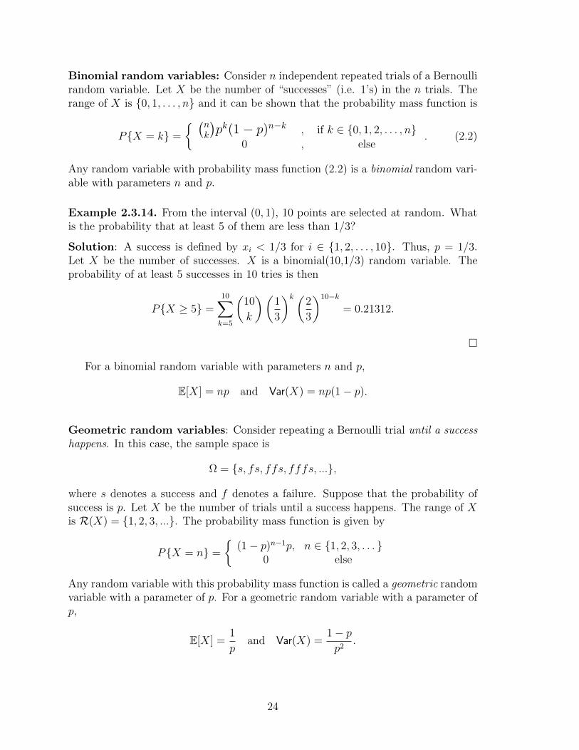
Binomial random variables: Consider n independent repeated trials of a Bernoullirandom variable. Let X be the number of “successes” (i.e. 1’s) in the n trials. Therange of X is 0, 1, . . . , n and it can be shown that the probability mass function is

PX = k =

nk

pk(1− p)n−k

, if k ∈ 0, 1, 2, . . . , n0 , else

. (2.2)

Any random variable with probability mass function (2.2) is a binomial random vari-able with parameters n and p.

Example 2.3.14. From the interval (0, 1), 10 points are selected at random. Whatis the probability that at least 5 of them are less than 1/3?

Solution: A success is defined by xi < 1/3 for i ∈ 1, 2, . . . , 10. Thus, p = 1/3.Let X be the number of successes. X is a binomial(10,1/3) random variable. Theprobability of at least 5 successes in 10 tries is then

PX ≥ 5 =10

k=5

10

k

1

3

k 2

3

10−k

= 0.21312.

For a binomial random variable with parameters n and p,

E[X] = np and Var(X) = np(1− p).

Geometric random variables: Consider repeating a Bernoulli trial until a successhappens. In this case, the sample space is

Ω = s, fs, ffs, fffs, ...,

where s denotes a success and f denotes a failure. Suppose that the probability ofsuccess is p. Let X be the number of trials until a success happens. The range of Xis R(X) = 1, 2, 3, .... The probability mass function is given by

PX = n =

(1− p)n−1p, n ∈ 1, 2, 3, . . .

0 else

Any random variable with this probability mass function is called a geometric randomvariable with a parameter of p. For a geometric random variable with a parameter ofp,

E[X] =1

pand Var(X) =

1− p

p2.

24

Geometric random variables, along with exponential random variables, have thememoryless property. Let X be a Geometric(p) random variable. Then for all n,m ≥1

PX > n+m | X > m =PX > n+mPX > m =

n+m failures to start

m failures to start

=(1− p)n+m

(1− p)m= (1− p)n = PX > n.

In words, this says that the probability that the next n trials will be failures, giventhat the first m trials were failures, is the same as the probability that first n arefailures.

Poisson random variables: This is one of the most important random variablesin the study of stochastic models of reaction networks and will arise time and timeagain in this class.

A random variable with range 0, 1, 2, . . . is a Poisson random variable with param-eter λ > 0 if

PX = k =

λke−λ

k! , k = 0, 1, 2, . . .

0 , else

.

For a Poisson random variable with a parameter of λ,

E[X] = λ and Var(X) = λ.

The Poisson random variable, together with the Poisson process, will play a centralrole in this class, especially when we discuss continuous time Markov chains. Thefollowing can be shown by, for example, generating functions.

Theorem 2.3.15. If X ∼ Poisson(λ) and Y ∼ Poisson(µ) then Z = X + Y ∼Poisson(λ+ µ).

The Poisson process. An increasing process on the integers Y (t) is said to be aPoisson process with intensity (or rate or propensity) λ if

1. Y (0) = 0.

2. The number of events in disjoint time intervals are independent.

3. PY (s+ t)− Y (t) = i = e−λs (λs)

i

i!, i = 0, 1, 2, . . . for any s, t ≥ 0

The Poisson process will be the main tool in the development of (pathwise) stochas-tic models of biochemical reaction systems in this class and will be derived morerigorously later.

25

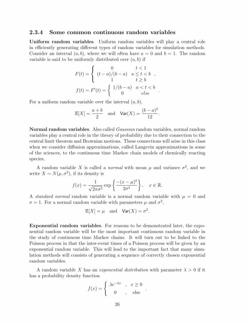
2.3.4 Some common continuous random variables

Uniform random variables. Uniform random variables will play a central rolein efficiently generating different types of random variables for simulation methods.Consider an interval (a, b), where we will often have a = 0 and b = 1. The randomvariable is said to be uniformly distributed over (a, b) if

F (t) =

0 t < 1(t− a)/(b− a) a ≤ t < b

1 t ≥ b

,

f(t) = F(t) =

1/(b− a) a < t < b

0 else.

For a uniform random variable over the interval (a, b),

E[X] =a+ b

2and Var(X) =

(b− a)2

12.

Normal random variables. Also called Gaussian random variables, normal randomvariables play a central role in the theory of probability due to their connection to thecentral limit theorem and Brownian motions. These connections will arise in this classwhen we consider diffusion approximations, called Langevin approximations in someof the sciences, to the continuous time Markov chain models of chemically reactingspecies.

A random variable X is called a normal with mean µ and variance σ2, and wewrite X ∼ N(µ, σ2), if its density is

f(x) =1√2πσ2

exp

−(x− µ)2

2σ2

, x ∈ R.

A standard normal random variable is a normal random variable with µ = 0 andσ = 1. For a normal random variable with parameters µ and σ2,

E[X] = µ and Var(X) = σ2.

Exponential random variables. For reasons to be demonstrated later, the expo-nential random variable will be the most important continuous random variable inthe study of continuous time Markov chains. It will turn out to be linked to thePoisson process in that the inter-event times of a Poisson process will be given by anexponential random variable. This will lead to the important fact that many simu-lation methods will consists of generating a sequence of correctly chosen exponentialrandom variables.

A random variable X has an exponential distribution with parameter λ > 0 if ithas a probability density function

f(x) =

λe−λx , x ≥ 0

0 , else.

26

For an exponential random variable with a parameter of λ > 0,

E[X] =1

λand Var(X) =

1

λ2.

Similar to the geometric random variable, the exponential random variable hasthe memoryless property.

Proposition 2.3.16 (Memoryless property). Let X ∼ Exp(λ), then for any s, t ≥ 0,

PX > (s+ t) | X > t = PX > s. (2.3)

Probably the most important role the exponential random variable will play inthese notes is as the inter-event time of Poisson random variables.

Proposition 2.3.17. Consider a Poisson process with rate λ > 0. Let Ti be the timebetween the ith and i+ 1st events. Then Ti ∼ Exp(λ).

The following propositions are relatively straightforward to prove and form theheart of the usual methods used to simulate continuous time Markov chains. Thismethod is often termed the Gillespie algorithm in the biochemical community, andwill be discussed later in the notes.

Proposition 2.3.18. If for i = 1, . . . , n, the random variables Xi ∼ Exp(λi) areindependent, then

X0 ≡ miniXi ∼ Exp(λ0), where λ0 =

n

i=1

λi.

Proof. Let X0 = miniXi. Set λ0 =

i λni=1. Then,

PX0 > t = PX1 > t, . . . , Xn > t =n

i=1

PXi > t =n

i=1

e−λit = e

−λ0t.

Proposition 2.3.19. For i = 1, . . . , n, let the random variables Xi ∼ Exp(λi) beindependent. Let j be the index of the smallest of the Xi. Then j is a discreterandom variable with probability mass function

Pj = i =λi

λ0, where λ0 =

n

i=1

λi.

27

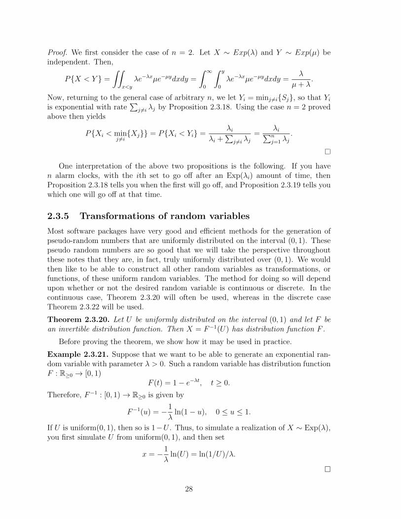
Proof. We first consider the case of n = 2. Let X ∼ Exp(λ) and Y ∼ Exp(µ) beindependent. Then,

PX < Y =

x<y

λe−λx

µe−µy

dxdy =

∞

0

y

0

λe−λx

µe−µy

dxdy =λ

µ+ λ.

Now, returning to the general case of arbitrary n, we let Yi = minj =iSj, so that Yi

is exponential with rate

j =i λj by Proposition 2.3.18. Using the case n = 2 provedabove then yields

PXi < minj =i

Xj = PXi < Yi =λi

λi +

j =i λj=

λinj=1 λj

.

One interpretation of the above two propositions is the following. If you haven alarm clocks, with the ith set to go off after an Exp(λi) amount of time, thenProposition 2.3.18 tells you when the first will go off, and Proposition 2.3.19 tells youwhich one will go off at that time.

2.3.5 Transformations of random variables

Most software packages have very good and efficient methods for the generation ofpseudo-random numbers that are uniformly distributed on the interval (0, 1). Thesepseudo random numbers are so good that we will take the perspective throughoutthese notes that they are, in fact, truly uniformly distributed over (0, 1). We wouldthen like to be able to construct all other random variables as transformations, orfunctions, of these uniform random variables. The method for doing so will dependupon whether or not the desired random variable is continuous or discrete. In thecontinuous case, Theorem 2.3.20 will often be used, whereas in the discrete caseTheorem 2.3.22 will be used.

Theorem 2.3.20. Let U be uniformly distributed on the interval (0, 1) and let F bean invertible distribution function. Then X = F−1(U) has distribution function F .

Before proving the theorem, we show how it may be used in practice.

Example 2.3.21. Suppose that we want to be able to generate an exponential ran-dom variable with parameter λ > 0. Such a random variable has distribution functionF : R≥0 → [0, 1)

F (t) = 1− e−λt

, t ≥ 0.

Therefore, F−1 : [0, 1) → R≥0 is given by

F−1(u) = −1

λln(1− u), 0 ≤ u ≤ 1.

If U is uniform(0, 1), then so is 1−U . Thus, to simulate a realization of X ∼ Exp(λ),you first simulate U from uniform(0, 1), and then set

x = −1

λln(U) = ln(1/U)/λ.

28

Proof. (of Theorem 2.3.20) Letting X = F−1(U) where U is uniform(0, 1), we have

PX ≤ t = PF−1(U) ≤ t= PU ≤ F (t)= F (t).

Theorem 2.3.22. Let U be uniformly distributed on the interval (0, 1). Suppose thatpk ≥ 0 for each k ∈ 0, 1, . . . , , and that

k pk = 1. Define

qk = PX ≤ k =k

i=0

pi.

LetX = mink | qk ≥ U.

Then,PX = k = pk.

Proof. Taking q−1 = 0, we have for any k ∈ 0, 1, . . . ,

PX = k = P qk−1 < U ≤ qk = qk − qk−1 = pk.

In practice, the above theorem is typically used by repeatedly checking whetheror not U ≤

ki=0 pi, and stopping the first time the inequality holds. We note that

the theorem is stated in the setting of an infinite state space, though the analogoustheorem holds in the finite state space case.

2.3.6 More than one random variable

To discuss more than one random variable defined on the same probability space(Ω,F , P ), we need joint distributions.

Definition 2.3.23. Let X1, . . . , Xn be discrete random variables with domain Ω.Then

pX1,...,Xn(x1, . . . , xn) = PX1 = x1, . . . , Xn = xnis called the joint probability mass function of X1, . . . , Xn.

Definition 2.3.24. We say that X1, . . . , Xn are jointly continuous if there exists afunction f(x1, . . . , xn), defined for all reals, such that for all A ⊂ Rn

P(X1, . . . , Xn) ∈ A =

· · ·

(x1,...,xn∈A)

f(x1, . . . , xn)dx1 . . . dxn.

The function f(x1, . . . , xn) is called the joint probability density function.

29

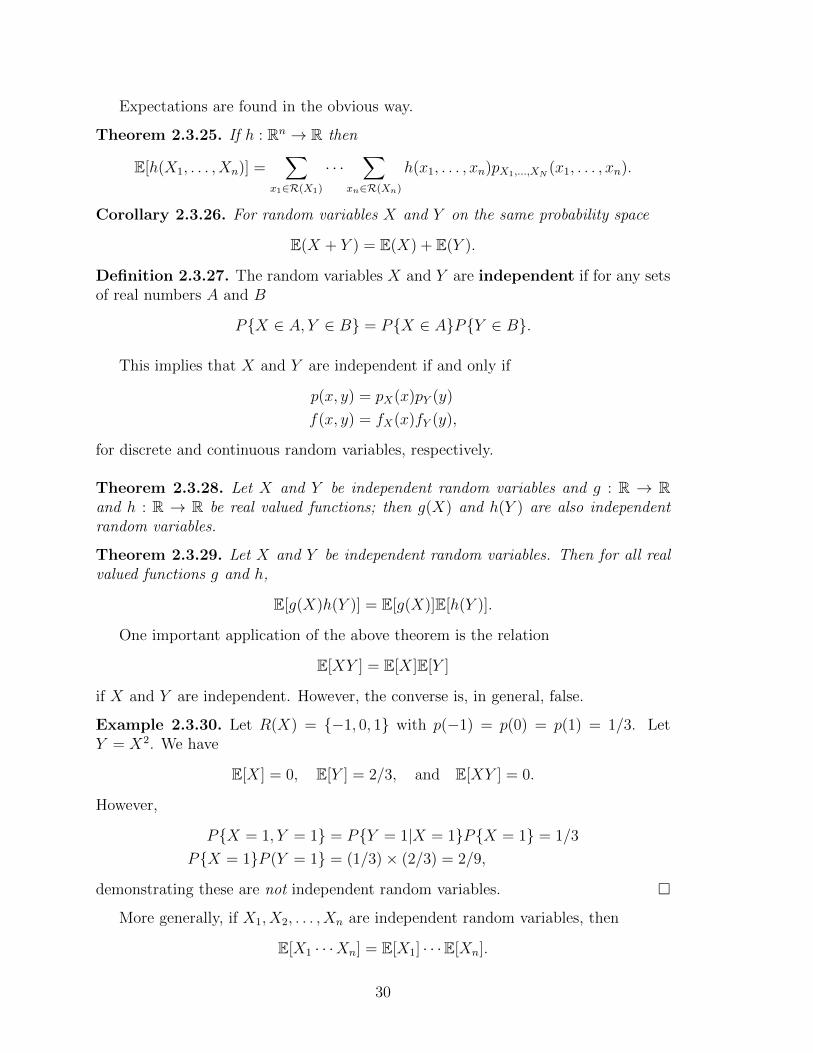
Expectations are found in the obvious way.

Theorem 2.3.25. If h : Rn → R then

E[h(X1, . . . , Xn)] =

x1∈R(X1)

· · ·

xn∈R(Xn)

h(x1, . . . , xn)pX1,...,XN (x1, . . . , xn).

Corollary 2.3.26. For random variables X and Y on the same probability space

E(X + Y ) = E(X) + E(Y ).

Definition 2.3.27. The random variables X and Y are independent if for any setsof real numbers A and B

PX ∈ A, Y ∈ B = PX ∈ APY ∈ B.

This implies that X and Y are independent if and only if

p(x, y) = pX(x)pY (y)

f(x, y) = fX(x)fY (y),

for discrete and continuous random variables, respectively.

Theorem 2.3.28. Let X and Y be independent random variables and g : R → Rand h : R → R be real valued functions; then g(X) and h(Y ) are also independentrandom variables.

Theorem 2.3.29. Let X and Y be independent random variables. Then for all realvalued functions g and h,

E[g(X)h(Y )] = E[g(X)]E[h(Y )].

One important application of the above theorem is the relation

E[XY ] = E[X]E[Y ]

if X and Y are independent. However, the converse is, in general, false.

Example 2.3.30. Let R(X) = −1, 0, 1 with p(−1) = p(0) = p(1) = 1/3. LetY = X2. We have

E[X] = 0, E[Y ] = 2/3, and E[XY ] = 0.

However,

PX = 1, Y = 1 = PY = 1|X = 1PX = 1 = 1/3

PX = 1P (Y = 1 = (1/3)× (2/3) = 2/9,

demonstrating these are not independent random variables. More generally, if X1, X2, . . . , Xn are independent random variables, then

E[X1 · · ·Xn] = E[X1] · · ·E[Xn].

30

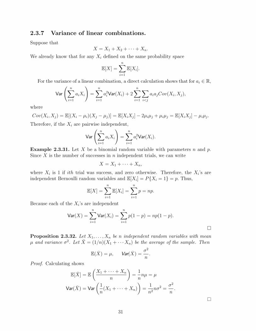
2.3.7 Variance of linear combinations.

Suppose thatX = X1 +X2 + · · ·+Xn.

We already know that for any Xi defined on the same probability space

E[X] =n

i=1

E[Xi].

For the variance of a linear combination, a direct calculation shows that for ai ∈ R,

Var

n

i=1

aiXi

=

n

i=1

a2iVar(Xi) + 2

n

i=1

i<j

aiajCov(Xi, Xj),

where

Cov(Xi, Xj) = E[(Xi − µi)(Xj − µj)] = E[XiXj]− 2µiµj + µiµj = E[XiXj]− µiµj.

Therefore, if the Xi are pairwise independent,

Var

n

i=1

aiXi

=

n

i=1

a2iVar(Xi).

Example 2.3.31. Let X be a binomial random variable with parameters n and p.Since X is the number of successes in n independent trials, we can write

X = X1 + · · ·+Xn,

where Xi is 1 if ith trial was success, and zero otherwise. Therefore, the Xi’s areindependent Bernoulli random variables and E[Xi] = PXi = 1 = p. Thus,

E[X] =n

i=1

E[Xi] =n

i=1

p = np.

Because each of the Xi’s are independent

Var(X) =n

i=1

Var(Xi) =n

i=1

p(1− p) = np(1− p).

Proposition 2.3.32. Let X1, . . . , Xn be n independent random variables with meanµ and variance σ2. Let X = (1/n)(X1 + · · ·Xn) be the average of the sample. Then

E(X) = µ, Var(X) =σ2

n.

Proof. Calculating shows

E[X] = EX1 + · · ·+Xn

n

=

1

nnµ = µ

Var(X) = Var

1

n(X1 + · · ·+Xn)

=

1

n2nσ

2 =σ2

n.

31

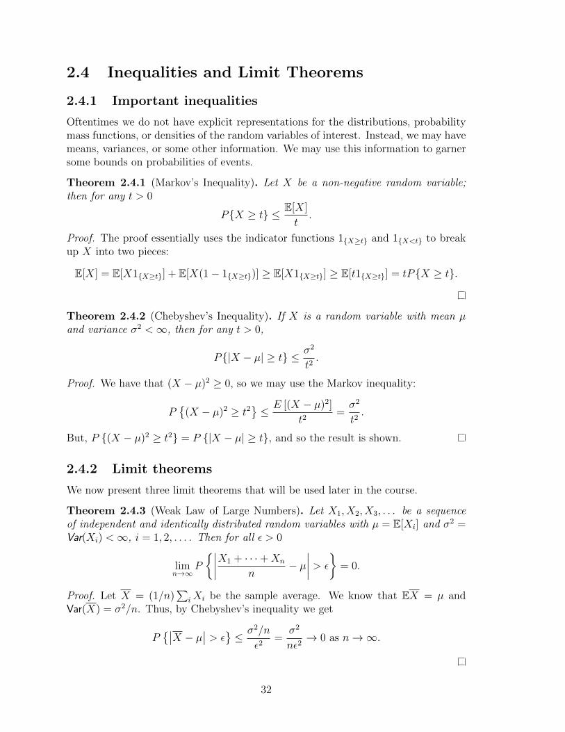
2.4 Inequalities and Limit Theorems

2.4.1 Important inequalities

Oftentimes we do not have explicit representations for the distributions, probabilitymass functions, or densities of the random variables of interest. Instead, we may havemeans, variances, or some other information. We may use this information to garnersome bounds on probabilities of events.

Theorem 2.4.1 (Markov’s Inequality). Let X be a non-negative random variable;then for any t > 0

PX ≥ t ≤ E[X]

t.

Proof. The proof essentially uses the indicator functions 1X≥t and 1X<t to breakup X into two pieces:

E[X] = E[X1X≥t] + E[X(1− 1X≥t)] ≥ E[X1X≥t] ≥ E[t1X≥t] = tPX ≥ t.

Theorem 2.4.2 (Chebyshev’s Inequality). If X is a random variable with mean µ

and variance σ2 < ∞, then for any t > 0,

P|X − µ| ≥ t ≤ σ2

t2.

Proof. We have that (X − µ)2 ≥ 0, so we may use the Markov inequality:

P(X − µ)2 ≥ t

2≤ E [(X − µ)2]

t2=

σ2

t2.

But, P (X − µ)2 ≥ t2 = P |X − µ| ≥ t, and so the result is shown.

2.4.2 Limit theorems

We now present three limit theorems that will be used later in the course.

Theorem 2.4.3 (Weak Law of Large Numbers). Let X1, X2, X3, . . . be a sequenceof independent and identically distributed random variables with µ = E[Xi] and σ2 =Var(Xi) < ∞, i = 1, 2, . . . . Then for all > 0

limn→∞

P

X1 + · · ·+Xn

n− µ

>

= 0.

Proof. Let X = (1/n)

i Xi be the sample average. We know that EX = µ andVar(X) = σ2/n. Thus, by Chebyshev’s inequality we get

PX − µ

> ≤ σ2/n

2=

σ2

n2→ 0 as n → ∞.

32

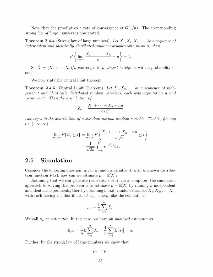
Note that the proof gives a rate of convergence of O(1/n). The correspondingstrong law of large numbers is now stated.

Theorem 2.4.4 (Strong law of large numbers). Let X1, X2, X3, . . . be a sequence ofindependent and identically distributed random variables with mean µ. then

P

limn→∞

X1 + · · ·+Xn

n= µ

= 1.

So X = (X1 + · · ·Xn)/n converges to µ almost surely, or with a probability ofone.

We now state the central limit theorem.

Theorem 2.4.5 (Central Limit Theorem). Let X1, X2, . . . be a sequence of inde-pendent and identically distributed random variables, each with expectation µ andvariance σ2. Then the distribution of

Zn =X1 + · · ·+Xn − nµ

σ√n

converges to the distribution of a standard normal random variable. That is, for anyt ∈ (−∞,∞)

limn→∞

PZn ≤ t = limn→∞

P

X1 + · · ·+Xn − nµ

σ√n

≤ t

=1√2π

t

−∞e−x2/2

dx.

2.5 Simulation

Consider the following question: given a random variable X with unknown distribu-tion function F (x), how can we estimate µ = E[X]?

Assuming that we can generate realizations of X via a computer, the simulationapproach to solving this problem is to estimate µ = E[X] by running n independentand identical experiments, thereby obtaining n i.i.d. random variablesX1, X2, . . . , Xn,with each having the distribution F (x). Then, take the estimate as

µn =1

n

n

i=1

Xi.

We call µn an estimator. In this case, we have an unbiased estimator as

Eµn =1

nE

n

i=1

Xi =1

n

n

i=1

E[Xi] = µ.

Further, by the strong law of large numbers we know that

µn → µ,

33

as n → ∞, with a probability of one.Of course, knowing that µn → µ, as n → ∞, does not actually tell us how large

of an n we need in practice. This brings us to the next logical question: how good isthe estimate for a given, finite n. To answer this question, we will apply the centrallimit theorem.

We know from the central limit theorem that

X1 +X2 + · · ·+Xn − nµ

σ√n

D≈ N(0, 1),

or √n

σ(µn − µ)

D≈ N(0, 1).

Specifically, for any z ∈ R

P −z ≤ N(0, 1) ≤ z ≈ P

−z ≤

√n

σ(µn − µ) ≤ z

= P

− σz√

n≤ (µn − µ) ≤ σz√

n

= P

µn −

σz√n≤ µ ≤ µn +

σz√n

.

In words, the above says that the probability that the true value, µ, is within ±σz/√n

of the estimator µn is P −z ≤ N(0, 1) ≤ z, which can be found for any z. Moreimportantly, a value z can be found for any desired level of confidence. The inter-val (µ − σz/

√n, µ + σz/

√n) is called our confidence interval and the probability

P −z ≤ N(0, 1) ≤ z is our confidence. Note that both our confidence and the sizeof the confidence interval increase as z is increased.

We now turn to finding the value z for a desired confidence level. Letting

Φ(z) = PN(0, 1) ≤ z =1√2π

z

−∞e−t2/2

dt,

we have

P−z ≤ N(0, 1) ≤ z = PN(0, 1) ≤ z− PN(0, 1) ≤ −z= Φ(z)− Φ(−z)

= Φ(z)− (1− Φ(z))

= 2Φ(z)− 1.

Therefore, if for some δ > 0 we want to have a probability of 1− δ that the true valueis in the constructed confidence interval, then we must choose z so that

P−z ≤ N(0, 1) ≤ z = 1− δ.

That is, we need to find a z so that

2Φ(z)− 1 = 1− δ,

34

or

Φ(z) = 1− δ

2.

For example, if δ = .1, so that a 90% confidence interval is required, then

Φ(z) = 1− .05 = .95,

and z = 1.65. If, on the other hand, we want δ = 0.05, so that a 95% confidenceinterval is desired, then

Φ(z) = 1− .025 = .975

and z = 1.96.Summarizing, we see that for a given δ, we can find a z so that the probability

that the parameter µ, which is what we are after, lies in the intervalµn −

σz√n, µn +

σz√n

is approximately 1− δ. Further, as n gets larger, the confidence interval shrinks. It isworth pointing out that the confidence interval shrinks at a rate of 1/

√n. Therefore,

to get a 10-fold increase accuracy, we need a 100-fold increase in work.There is a major problem with the preceding arguments: if we don’t know µ,

which is what we are after, we most likely do not know σ either. Therefore, we willalso need to estimate it from our independent samples X1, X2, . . . , Xn.

Theorem 2.5.1. Let X1, . . . , Xn be independent and identical samples with mean µ

and variance σ2, and let

σ2n =

1

n− 1

n

i=1

(Xi − µn)2,

where µn is the sample mean

µn =1

n

n

i=1

Xi.

Then,Eσ2

n = σ2.

Proof. We have

Eσ2n = E

1

n− 1

n

i=1

(Xi − µn)2

,

which yields

(n− 1)Eσ2n = E

n

i=1

(Xi − µn)2

=

n

i=1

E[X2i ]− 2E

µn

n

i=1

Xi

+ nE

µ2n

=n

i=1

E[X2i ]− 2E [µnnµn] + nE

µ2n

= nE[X2]− nEµ2n

.

35

However,

Eµ2n

= Var(µn) + E [µn]

2 = Var

1

n

n

i=1

Xi

+ µ

2 =1

nσ2 + µ

2.

Therefore,

n− 1

nEσ2

n = E[X2]− E[µ2n] =

σ2 + µ

2−

1

nσ2 + µ

=

n− 1

nσ2,

completing the proof.

Therefore, we can useσn =

σ2n

as an estimate of the standard deviation in the confidence interval andµn −

σnz√n, µn +

σnz√n

is an approximate (1− δ)100% confidence interval for µ = E[X].We note that there are two sources of error in the development of the above

confidence interval that we will not explore here. First, there is the question of howgood an approximation the central limit theorem is giving us. For reasonably sizedn, this should not give too much of an error. The second source of error is in usingσn as opposed to σ. Again, for large n, this error will be relatively small.

We have the following algorithm for producing a confidence interval for an expec-tation given a number of realizations.

Algorithm for producing confidence intervals for a given n.

1. Select n, the number of experiments to be run, and δ > 0.

2. Perform n independent replications of the experiment, obtaining the observa-tions X1, X2, . . . , Xn of the random variable X.

3. Compute the sample mean and sample variance

µn =1

n(X1 + · · ·+Xn)

σ2n =

1

n− 1

n

i=1

(Xi − µn)2.

4. Select z such that Φ(z) = 1−δ/2. Then an approximate (1−δ)100% confidenceinterval for µ = E[X] is

µn −

σnz√n, µn +

σnz√n

.

36

If a level of precision is desired, and n is allowed to depend upon δ and a tolerance, then the following algorithm is most useful.

Algorithm for producing confidence intervals to a given tolerance.

1. Select δ > 0, determining the desired confidence, and > 0 giving the desiredprecision. Select z such that Φ(z) = 1− δ/2.

2. Perform independent replications of the experiment, obtaining the observationsX1, X2, . . . , Xn of the random variable X, until

σnz√n

< .

3. Report

µn =1

n(X1 + · · ·+Xn)

and the (1− δ)100% confidence interval for µ = E[X],µn −

σnz√n, µn +

σnz√n

≈ [µ− , µ+ ] .

There are two conditions usually added to the above algorithm. First, thereis normally some minimal number of samples generated, n0 say, before one checkswhether or not σnz/

√n < . Second, it can be time consuming to compute the

standard deviation after every generation of a new iterate. Therefore, one normallyonly does so after every multiple of M iterates, for some positive integer M > 0. Wewill not explore the question of what “good” values of n0 and M are, though takingn0 = M ≈ 100 is usually sufficient.

2.6 Exercises

1. Verify, through a direct calculation, Equation (2.1).

2. Verify the memoryless property, Equation (2.3), for exponential random vari-ables.

3. Matlab exercise. Perform the following tasks using Matlab.

(a) Using a FOR LOOP, use the etime command to time how long it takesMatlab to generate 100,000 exponential random variables with a parameterof 1/10 using the built-in exponential random number generator. Samplecode for this procedure is provided on the course website.

(b) Again using a FOR LOOP, use the etime command to time how longit takes Matlab to generate 100,000 exponential random variables withparameter 1/10 using the transformation method given in Theorem 2.3.20.

37

4. Matlab exercise. Let X be a random variable with range −10, 0, 1, 4, 12and probability mass function

PX = −10 =1

5, PX = 0 =

1

8, PX = 1 =

1

4,

PX = 4 =1

3, PX = 12 =

11

120.

Using Theorem 2.3.22, generate N independent copies of X and use them toestimate EX via

EX ≈ 1

N

N

i=1

X[i],

where X[i] is the ith independent copy of X and N ∈ 100, 103, 104, 105. Com-pare the result for eachN to the actual expected value. A helpful sample Matlabcode has been provided on the course website.

38