Chapter 2 Bayes’ Theorem for Distributionsnlf8/teaching/mas2317/notes/chapter2.pdf · Chapter 2 Bayes’ Theorem for Distributions 2.1 Introduction Suppose we have data xwhich we

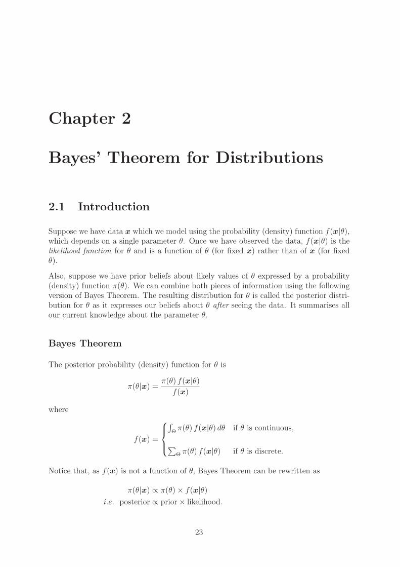
Chapter 2

Bayes’ Theorem for Distributions

2.1 Introduction

Suppose we have data x which we model using the probability (density) function f(x|θ),which depends on a single parameter θ. Once we have observed the data, f(x|θ) is thelikelihood function for θ and is a function of θ (for fixed x) rather than of x (for fixedθ).

Also, suppose we have prior beliefs about likely values of θ expressed by a probability(density) function π(θ). We can combine both pieces of information using the followingversion of Bayes Theorem. The resulting distribution for θ is called the posterior distri-bution for θ as it expresses our beliefs about θ after seeing the data. It summarises allour current knowledge about the parameter θ.

Bayes Theorem

The posterior probability (density) function for θ is

π(θ|x) = π(θ) f(x|θ)f(x)

where

f(x) =

∫

Θπ(θ) f(x|θ) dθ if θ is continuous,

∑

Θ π(θ) f(x|θ) if θ is discrete.

Notice that, as f(x) is not a function of θ, Bayes Theorem can be rewritten as

π(θ|x) ∝ π(θ)× f(x|θ)i.e. posterior ∝ prior× likelihood.

23

24 CHAPTER 2. BAYES’ THEOREM FOR DISTRIBUTIONS

Thus, to obtain the posterior distribution, we need:

(1) data, from which we can form the likelihood f(x|θ), and

(2) a suitable distribution, π(θ), that represents our prior beliefs about θ.

You should now be comfortable with how to obtain the likelihood (point 1 above; seeSection 1.3 of these notes, plus MAS1342 and MAS2302!). But how do we specify a prior(point 2)? In Chapter 3 we will consider the task of prior elicitation – the process whichfacilitates the ‘derivation’ of a suitable prior distribution for θ. For now, we will assumesomeone else has done this for us; the main aim of this chapter is simply to operateBayes’ Theorem for distributions to obtain the posterior distribution for θ. And beforewe do this, it will be worth re–familiarising ourselves with some continuous probabilitydistributions you have met before, and which we will use extensively in this course: theuniform, beta and gamma distributions (indeed, I will assume that you are more thanfamiliar with some other ‘standard’ distributions we will use – e.g. the exponential,Normal, Poisson, and binomial, and so will not review these here).

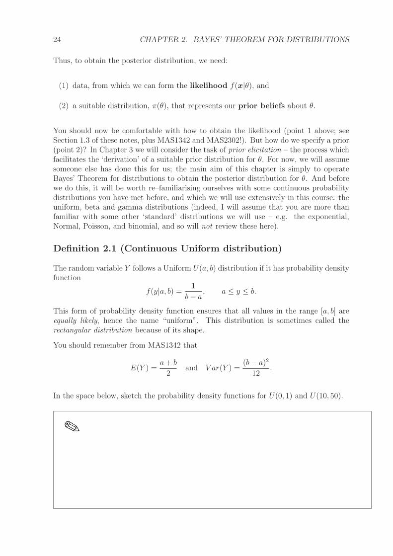
Definition 2.1 (Continuous Uniform distribution)

The random variable Y follows a Uniform U(a, b) distribution if it has probability densityfunction

f(y|a, b) = 1

b− a, a ≤ y ≤ b.

This form of probability density function ensures that all values in the range [a, b] areequally likely, hence the name “uniform”. This distribution is sometimes called therectangular distribution because of its shape.

You should remember from MAS1342 that

E(Y ) =a+ b

2and V ar(Y ) =

(b− a)2

12.

In the space below, sketch the probability density functions for U(0, 1) and U(10, 50).

✎

2.1. INTRODUCTION 25

Definition 2.2 (Beta distribution)

The random variable Y follows a Beta Be(a, b) distribution (a > 0, b > 0) if it hasprobability density function

f(y|a, b) = ya−1(1− y)b−1

B(a, b), 0 < y < 1. (2.1)

The constant term B(a, b), also known as the beta function, ensures that the densityintegrates to one. Therefore

B(a, b) =

∫ 1

0

ya−1(1− y)b−1 dy. (2.2)

It can be shown that the beta function can be expressed in terms of another function,called the gamma function Γ(·), as

B(a, b) =Γ(a)Γ(b)

Γ(a+ b),

where

Γ(a) =

∫ ∞

0

xa−1e−x dx. (2.3)

Tables are available for both B(a, b) and Γ(a). However, these functions are very simpleto evaluate when a and b are integers since the gamma function is a generalisation of thefactorial function. In particular, when a and b are integers, we have

Γ(a) = (a− 1)! and B(a, b) =(a− 1)!(b− 1)!

(a+ b− 1)!.

For example,

B(2, 3) =1!× 2!

4!=

1

12.

It can be shown, using the identity Γ(a) = (a− 1)Γ(a− 1), that

E(Y ) =a

a+ b, and V ar(Y ) =

ab

(a+ b)2(a+ b+ 1).

Also

Mode(Y ) =a− 1

a+ b− 2, if a > 1 and b > 1.

Definition 2.3 (Gamma distribution)

The random variable Y follows a Gamma Ga(a, b) distribution (a > 0, b > 0) if it hasprobability density function

f(y|a, b) = baya−1e−by

Γ(a), y > 0,


where Γ(a) is the gamma function defined in (2.3). It can be shown that

E(Y ) =a

band V ar(Y ) =

a

b2.

Also

Mode(Y ) =a− 1

b, if a ≥ 1.

We can use R to visualise the beta and gamma distributions for various values of (a, b)(and indeed any other standard probability distribution you have met so far). Forexample, we know that the beta distribution is valid for all values in the range (0, 1). InR, we can set this up by typing:

> x=seq(0,1,0.01)

which specifies x to take all values in the range 0 to 1, in steps of 0.01. The followingcode then calculates the density of Be(2, 5), as given by Equation (2.1) with a = 2 andb = 5:

> y=dbeta(x,2,5)

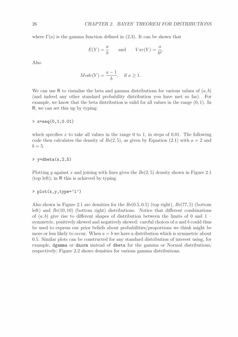
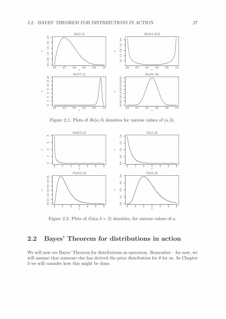
Plotting y against x and joining with lines gives the Be(2, 5) density shown in Figure 2.1(top left); in R this is achieved by typing

> plot(x,y,type=’l’)

Also shown in Figure 2.1 are densities for the Be(0.5, 0.5) (top right), Be(77, 5) (bottomleft) and Be(10, 10) (bottom right) distributions. Notice that different combinationsof (a, b) give rise to different shapes of distribution between the limits of 0 and 1 –symmetric, positively skewed and negatively skewed: careful choices of a and b could thusbe used to express our prior beliefs about probabilities/proportions we think might bemore or less likely to occur. When a = b we have a distribution which is symmetric about0.5. Similar plots can be constructed for any standard distribution of interest using, forexample, dgamma or dnorm instead of dbeta for the gamma or Normal distributions,respectively; Figure 2.2 shows densities for various gamma distributions.

2.2. BAYES’ THEOREM FOR DISTRIBUTIONS IN ACTION 27

02

46

810

12

14

xx

xx

yy

yy

0.0

0.00.0

0.0

0.0

0.0

0.20.2

0.20.2

0.40.4

0.40.4

0.60.6

0.60.6

0.80.8

0.80.8

1.0

1.01.0

1.0

1.0

1.0

1.0

1.5

1.5

1.5

2.0

2.0

2.0

2.5

2.5

2.5

3.0

3.0

0.5

0.5

3.5

Be(2, 5) Be(0.5, 0.5)

Be(77, 5) Be(10, 10)

Figure 2.1: Plots of Be(a, b) densities for various values of (a, b).

00

0

0

0

11

11

22

2

2

2

33

33

44

4

4

4

55

55

66

6

6

6

8

xx

xx

yy

yy

0.0

0.0

0.0

0.1

0.1

0.2

0.2

0.3

0.3

0.4

0.4

0.6

1.0

1.5

2.0

0.5

0.5

Ga(0.5, 2) Ga(1, 2)

Ga(2.5, 2) Ga(5, 2)

Figure 2.2: Plots of Ga(a, b = 2) densities, for various values of a.

2.2 Bayes’ Theorem for distributions in action

We will now see Bayes’ Theorem for distributions in operation. Remember – for now, wewill assume that someone else has derived the prior distribution for θ for us. In Chapter3 we will consider how this might be done.


Example 2.1

Consider an experiment with a possibly biased coin. Let θ = Pr(Head). Suppose that,before conducting the experiment, we believe that all values of θ are equally likely: thisgives a prior distribution θ ∼ U(0, 1), and so

π(θ) = 1, 0 < θ < 1. (2.4)

Note that with this prior distribution E(θ) = 0.5. We now toss the coin 5 times andobserve 1 head. Determine the posterior distribution for θ given this data.

Solution✎...Solution to Example 2.1... The data is an observation on the random variableX|θ ∼ Bin(5, θ). This gives a likelihood function

L(θ|x = 1) = f(x = 1|θ) = 5θ(1− θ)4 (2.5)

which favours values of θ near its maximum θ = 0.2. Therefore, we have a conflict ofopinions: the prior distribution (2.4) suggests that θ is probably around 0.5 and the data(2.5) suggest that it is around 0.2. We can use Bayes Theorem to combine these twosources of information in a coherent way. First


Solution✎...Solution to Example 2.1 continued...

f(x = 1) =

∫

Θ

π(θ)L(θ|x = 1) dθ (2.6)

=

∫ 1

0

1× 5θ(1− θ)4 dθ

=

∫ 1

0

θ × 5(1− θ)4 dθ

=[

−(1− θ)5 θ]1

0+

∫ 1

0

(1− θ)5 dθ

= 0 +

[

−(1− θ)6

6

]1

0

=1

6.

Therefore, the posterior density is

π(θ|x = 1) =π(θ)L(θ|x = 1)

f(x = 1)

=5θ(1− θ)4

1/6, 0 < θ < 1

= 30 θ(1− θ)4, 0 < θ < 1

=θ(1− θ)4

B(2, 5), 0 < θ < 1,

and so the posterior distribution is θ|x = 1 ∼ Be(2, 5) – see Definition 2.2. This distribu-tion has its mode at θ = 0.2, and mean at E[θ|x = 1] = 2/7 = 0.286.


The main difficulty in calculating the posterior distribution was in obtaining the f(x)term (2.6). However, in many cases we can recognise the posterior distribution withoutthe need to calculate this constant term (constant with respect to θ). In this example,we can calculate the posterior distribution as

π(θ|x) ∝ π(θ)f(x = 1|θ)∝ 1× 5θ(1− θ)4, 0 < θ < 1

= kθ(1− θ)4, 0 < θ < 1.

As θ is a continuous quantity, what we would like to know is what continuous distributiondefined on (0, 1) has a probability density function which takes the form kθg−1(1−θ)h−1.The answer is the Be(g, h) distribution. Therefore, choosing g and h appropriately, wecan see that the posterior distribution is θ|x = 1 ∼ Be(2, 5).

Summary:

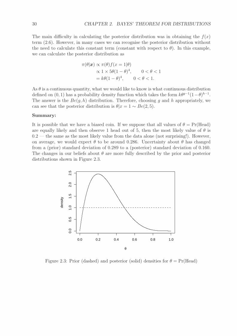
It is possible that we have a biased coin. If we suppose that all values of θ = Pr(Head)are equally likely and then observe 1 head out of 5, then the most likely value of θ is0.2 — the same as the most likely value from the data alone (not surprising!). However,on average, we would expect θ to be around 0.286. Uncertainty about θ has changedfrom a (prior) standard deviation of 0.289 to a (posterior) standard deviation of 0.160.The changes in our beliefs about θ are more fully described by the prior and posteriordistributions shown in Figure 2.3.

0.0 0.2 0.4 0.6 0.8 1.0

0.0

0.5

1.0

1.5

2.0

2.5

θ

dens

ity

Figure 2.3: Prior (dashed) and posterior (solid) densities for θ = Pr(Head)


Example 2.2

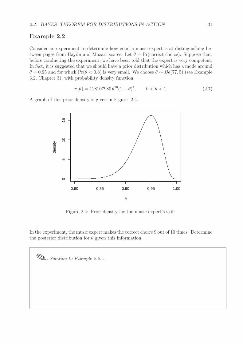
Consider an experiment to determine how good a music expert is at distinguishing be-tween pages from Haydn and Mozart scores. Let θ = Pr(correct choice). Suppose that,before conducting the experiment, we have been told that the expert is very competent.In fact, it is suggested that we should have a prior distribution which has a mode aroundθ = 0.95 and for which Pr(θ < 0.8) is very small. We choose θ ∼ Be(77, 5) (see Example3.2, Chapter 3), with probability density function

π(θ) = 128107980 θ76(1− θ)4, 0 < θ < 1. (2.7)

A graph of this prior density is given in Figure 2.4.

0.80 0.85 0.90 0.95 1.00

05

1015

θ

dens

ity

Figure 2.4: Prior density for the music expert’s skill.

In the experiment, the music expert makes the correct choice 9 out of 10 times. Determinethe posterior distribution for θ given this information.

✎...Solution to Example 2.2...


Solution

✎...Solution to Example 2.2 continued...We have an observation on the random variable X|θ ∼ Bin(10, θ). This gives a likelihoodfunction of

L(θ|x = 9) = f(x = 9|θ) = 10 θ9(1− θ) (2.8)

which favours values of θ near its maximum θ = 0.9. We combine these two sources ofinformation using Bayes Theorem. The posterior density function is

π(θ|x = 9) ∝ π(θ)L(θ|x = 9)

∝ 128107980 θ76(1− θ)4 × 10 θ9(1− θ), 0 < θ < 1

= kθ85(1− θ)5, 0 < θ < 1. (2.9)

We can recognise this density function as one from the Beta family. Whence, the posteriordistribution is θ|x = 9 ∼ Be(86, 6).


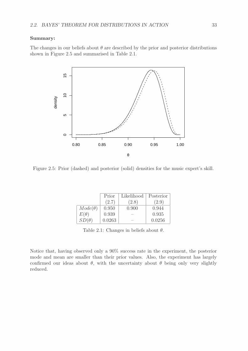
Summary:

The changes in our beliefs about θ are described by the prior and posterior distributionsshown in Figure 2.5 and summarised in Table 2.1.

0.80 0.85 0.90 0.95 1.00

05

1015

θ

dens

ity

Figure 2.5: Prior (dashed) and posterior (solid) densities for the music expert’s skill.

Prior Likelihood Posterior(2.7) (2.8) (2.9)

Mode(θ) 0.950 0.900 0.944E(θ) 0.939 – 0.935SD(θ) 0.0263 – 0.0256

Table 2.1: Changes in beliefs about θ.

Notice that, having observed only a 90% success rate in the experiment, the posteriormode and mean are smaller than their prior values. Also, the experiment has largelyconfirmed our ideas about θ, with the uncertainty about θ being only very slightlyreduced.


Example 2.3

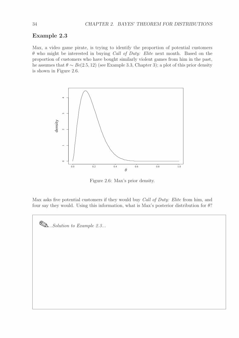
Max, a video game pirate, is trying to identify the proportion of potential customersθ who might be interested in buying Call of Duty: Elite next month. Based on theproportion of customers who have bought similarly violent games from him in the past,he assumes that θ ∼ Be(2.5, 12) (see Example 3.3, Chapter 3); a plot of this prior densityis shown in Figure 2.6.

01

23

4

0.0 0.2 0.4 0.6 0.8 1.0

θ

density

Figure 2.6: Max’s prior density.

Max asks five potential customers if they would buy Call of Duty: Elite from him, andfour say they would. Using this information, what is Max’s posterior distribution for θ?



Solution✎...Solution to Example 2.3 continued...We have been told that the prior for θ is a Be(2.5, 12) distribution – this has density givenby

1

B(2.5, 12)θ2.5−1(1− θ)12−1 = 435.1867θ1.5(1− θ)11. (2.10)

We have an observation on the random variable X|θ ∼ Bin(5, θ). This gives a likelihoodfunction of

L(θ|x = 4) = f(x = 4|θ) = 5C4θ4(1− θ)1 = 5θ4(1− θ), (2.11)

which favours values of θ near its maximum 0.8. We combine our prior information (2.10)with the data (2.11) – to obtain our posterior distribution – using Bayes’ Theorem. Theposterior density function is

π(θ|x = 4) ∝ π(θ)L(θ|x = 4)

∝ 435.1867θ1.5(1− θ)11 × 5θ4(1− θ), 0 < θ < 1,

givingπ(θ|x = 4) = kθ5.5(1− θ)12, 0 < θ < 1. (2.12)

You should recognise this density function as one from the beta family. In fact, we havea Be(6.5, 13), i.e. θ|x = 4 ∼ Be(6.5, 13).


Summary:

The changes in our beliefs about θ are described by the prior and posterior distributionsshown in Figure 2.7 and summarised in Table 2.2.

density

θ

01

23

4

0.0 0.2 0.4 0.6 0.8 1.0

Figure 2.7: Prior (dashed) and posterior (solid) densities for Max’s problem.


Mode(θ) 0.12 0.8 0.314E(θ) 0.172 – 0.333SD(θ) 0.096 – 0.104


Notice how the posterior has been “pulled” from the prior towards the observed value:the mode has moved up from 0.12 to 0.314, and the mean has moved up from 0.172to 0.333. Having just one observation in the likelihood, we see that there is hardlyany change in the standard deviation from prior to posterior: we would expect to see adecrease in standard deviation with the addition of more data values.


Example 2.4

Table 2.3 shows some data on the times between serious earthquakes. An earthquakeis included if its magnitude is at least 7.5 on the Richter scale or if over 1000 peoplewere killed. Recording starts on 16 December 1902 (4500 killed in Turkistan). The tableincludes data on 21 earthquakes, that is, 20 “waiting times” between earthquakes.

840 157 145 44 33 121 150 280 434 736584 887 263 1901 695 294 562 721 76 710

Table 2.3: Time intervals between major earthquakes (in days).

It is believed that earthquakes happen in a random haphazard kind of way and thattimes between earthquakes can be described by an exponential distribution. Data overa much longer period suggest that this exponential assumption is plausible. Therefore,we will assume that these data are a random sample from an exponential distributionwith rate θ (and mean 1/θ). The parameter θ describes the rate at which earthquakesoccur.

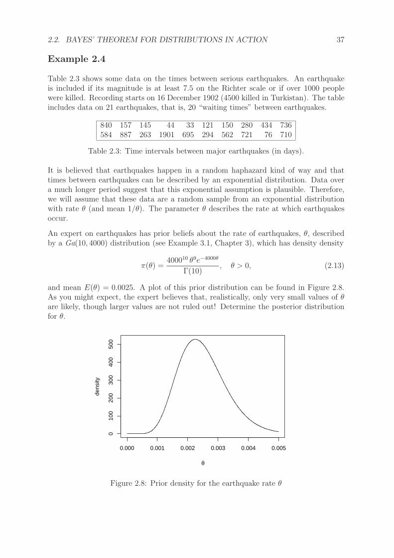
An expert on earthquakes has prior beliefs about the rate of earthquakes, θ, describedby a Ga(10, 4000) distribution (see Example 3.1, Chapter 3), which has density density

π(θ) =400010 θ9e−4000θ

Γ(10), θ > 0, (2.13)

and mean E(θ) = 0.0025. A plot of this prior distribution can be found in Figure 2.8.As you might expect, the expert believes that, realistically, only very small values of θare likely, though larger values are not ruled out! Determine the posterior distributionfor θ.

0.000 0.001 0.002 0.003 0.004 0.005

010

020

030

040

050

0

θ

dens

ity

Figure 2.8: Prior density for the earthquake rate θ


Solution

✎...Solution to Example 2.4... The data are observations on Xi|θ ∼ Exp(θ), i =1, 2, . . . , 20 (independent). Therefore, the likelihood function for θ is

L(θ|x) = f(x|θ) =20∏

i=1

θe−θxi , θ > 0

= θ20 exp

(

−θ20∑

i=1

xi

)

, θ > 0

= θ20e−9633θ, θ > 0. (2.14)

We now apply Bayes Theorem to combine the expert opinion with the observed data.The posterior density function is

π(θ|x) ∝ π(θ)L(θ|x)

∝ 400010 θ9e−4000θ

Γ(10)× θ20e−9633θ, θ > 0

= k θ30−1e−13633θ, θ > 0. (2.15)

The only continuous distribution which takes the form kθg−1e−hθ, θ > 0 is the Ga(g, h)distribution. Therefore, the posterior distribution must be θ|x ∼ Ga(30, 13633).


Summary:

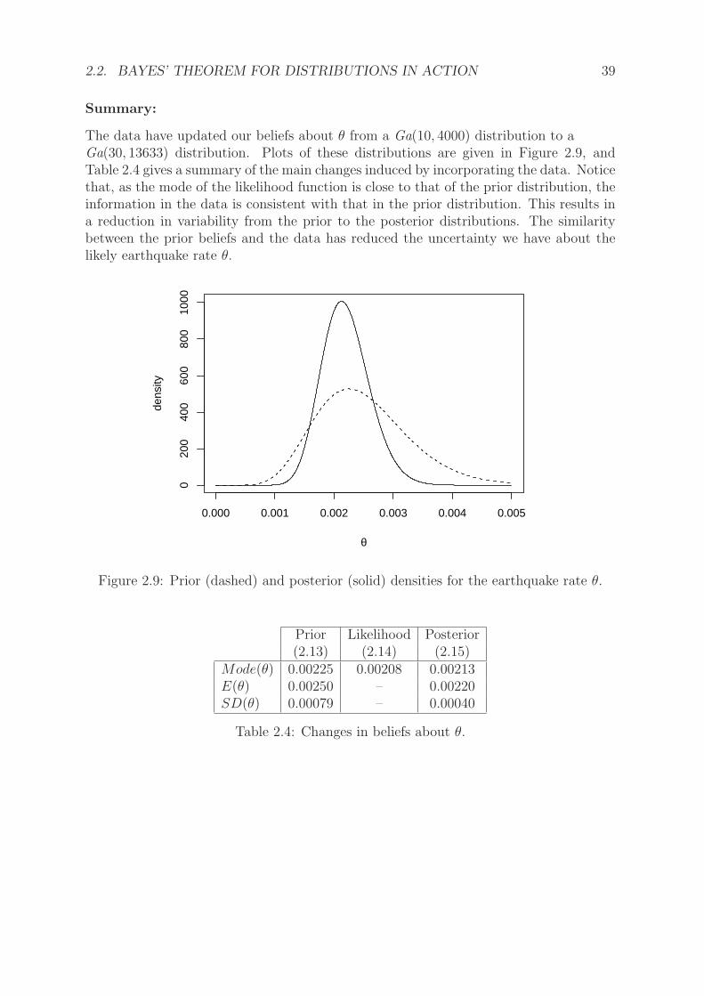
The data have updated our beliefs about θ from a Ga(10, 4000) distribution to aGa(30, 13633) distribution. Plots of these distributions are given in Figure 2.9, andTable 2.4 gives a summary of the main changes induced by incorporating the data. Noticethat, as the mode of the likelihood function is close to that of the prior distribution, theinformation in the data is consistent with that in the prior distribution. This results ina reduction in variability from the prior to the posterior distributions. The similaritybetween the prior beliefs and the data has reduced the uncertainty we have about thelikely earthquake rate θ.

0.000 0.001 0.002 0.003 0.004 0.005

020

040

060

080

010

00

θ

dens

ity

Figure 2.9: Prior (dashed) and posterior (solid) densities for the earthquake rate θ.


Mode(θ) 0.00225 0.00208 0.00213E(θ) 0.00250 – 0.00220SD(θ) 0.00079 – 0.00040



Example 2.5

We now consider the general case of the problem discussed in Example 2.4. SupposeXi|θ ∼ Exp(θ), i = 1, 2, . . . , n (independent) and our prior beliefs about θ are summarisedby a Ga(g, h) distribution (with g and h known), with density

π(θ) =hg θg−1e−hθ

Γ(g), θ > 0. (2.16)

Determine the posterior distribution for θ.

Solution

✎...Solution to Example 2.5...The likelihood function for θ is

L(θ|x) = f(x|θ) =n∏

i=1

θe−θxi , θ > 0

= θne−nx̄θ, θ > 0. (2.17)

We now apply Bayes Theorem. The posterior density function is

π(θ|x) ∝ π(θ)L(θ|x)

∝ hg θg−1e−hθ

Γ(g)× θne−nx̄θ, θ > 0.

π(θ|x) = kθg+n−1e−(h+nx̄)θ, θ > 0. (2.18)

where k is a constant that does not depend on θ. Therefore, the posterior distributiontakes the form kθg−1e−hθ, θ > 0 and so must be a gamma distribution. Thus we haveθ|x ∼ Ga(g + n, h+ nx̄).


Summary:

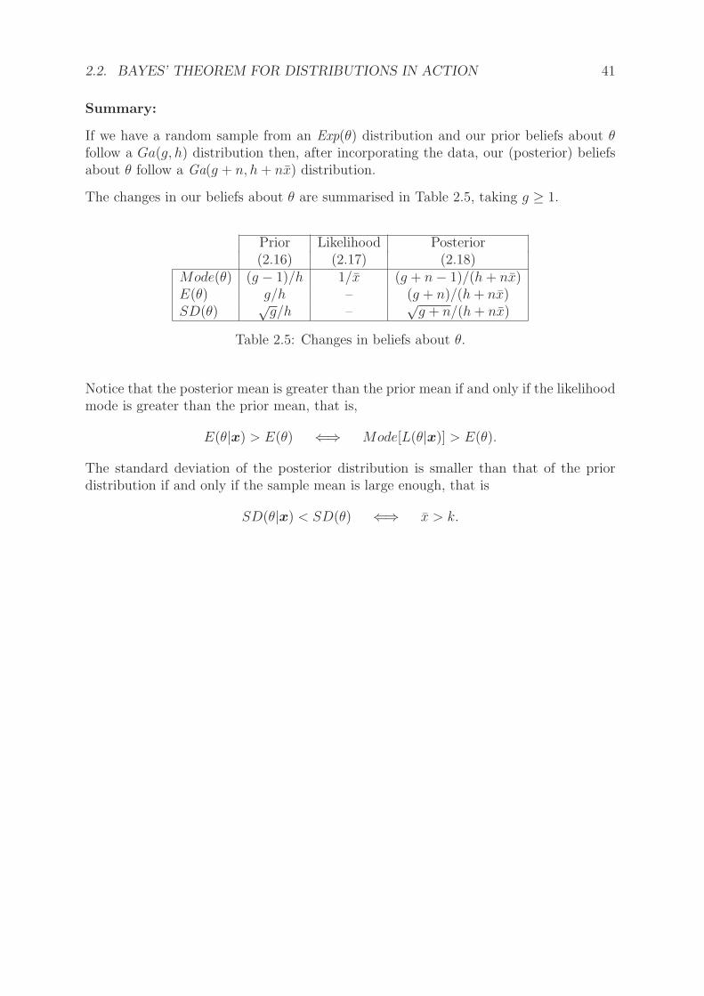
If we have a random sample from an Exp(θ) distribution and our prior beliefs about θfollow a Ga(g, h) distribution then, after incorporating the data, our (posterior) beliefsabout θ follow a Ga(g + n, h+ nx̄) distribution.

The changes in our beliefs about θ are summarised in Table 2.5, taking g ≥ 1.


Mode(θ) (g − 1)/h 1/x̄ (g + n− 1)/(h+ nx̄)E(θ) g/h – (g + n)/(h+ nx̄)SD(θ)

√g/h –

√g + n/(h+ nx̄)


Notice that the posterior mean is greater than the prior mean if and only if the likelihoodmode is greater than the prior mean, that is,

E(θ|x) > E(θ) ⇐⇒ Mode[L(θ|x)] > E(θ).

The standard deviation of the posterior distribution is smaller than that of the priordistribution if and only if the sample mean is large enough, that is

SD(θ|x) < SD(θ) ⇐⇒ x̄ > k.


Example 2.6

Suppose we have a random sample from a normal distribution. In Bayesian statistics,when dealing with the normal distribution, the mathematics is more straightforward ifwe work with the precision (= 1/variance) of the distribution rather than the varianceitself. So we will assume that this population has unknown mean µ but known precision τ :Xi|µ ∼ N(µ, 1/τ), i = 1, 2, . . . , n (independent), where τ is known. Suppose our priorbeliefs about µ can be summarised by a N(b, 1/d) distribution, with probability densityfunction

π(µ) =

(

d

2π

)1/2

exp

{

−d2(µ− b)2

}

. (2.19)

Determine the posterior distribution for µ.



Solution

✎...Solution to Example 2.6 continued...The likelihood function for µ is

L(µ|x) = f(x|µ) =n∏

i=1

( τ

2π

)1/2

exp{

−τ2(xi − µ)2

}

=( τ

2π

)n/2

exp

{

−τ2

n∑

i=1

(xi − µ)2

}

=( τ

2π

)n/2

exp

{

−τ2

n∑

i=1

(xi − x̄+ x̄− µ)2

}

=( τ

2π

)n/2

exp

{

−τ2

[

n∑

i=1

(xi − x̄)2 + n(x̄− µ)2

]}

Let

s2 =1

n

n∑

i=1

(xi − x̄)2

and then

L(µ|x) =( τ

2π

)n/2

exp{

−nτ2

[

s2 + (x̄− µ)2]

}

. (2.20)

Applying Bayes Theorem, the posterior density function is

π(µ|x) ∝ π(µ)L(µ|x)

∝(

d

2π

)1/2

exp

{

−d2(µ− b)2

}

×( τ

2π

)n/2

exp{

−nτ2

[

s2 + (x̄− µ)2]

}

= k1 exp

{

−1

2

[

d(µ− b)2 + nτ(x̄− µ)2]

}

where k1 is a constant that does not depend on µ. Now the exponent can be simplifiedby expanding terms in µ and then completing the square, as follows.


Solution

✎...Solution to Example 2.6 continued...We have

d(µ− b)2 + nτ(x̄− µ)2

= d(µ2 − 2bµ+ b2) + nτ(x̄2 − 2x̄µ+ µ2)

= (d+ nτ)µ2 − 2(db+ nτx̄)µ+ db2 + nτx̄2

= (d+ nτ)

{

µ−(

db+ nτx̄

d+ nτ

)}2

+ c

where c does not depend on µ. Let

B =db+ nτx̄

d+ nτand D = d+ nτ. (2.21)

Then

π(µ|x) = k1 exp

{

−D2(µ−B)2 − c

2

}

= k exp

{

−D2(µ−B)2

}

, (2.22)

where k is a constant that does not depend on µ. Therefore, the posterior distributiontakes the form k exp{−D(µ−B)2/2}, −∞ < µ <∞ and so must be a normal distribution:we have µ|x ∼ N(B, 1/D).


Summary:

If we have a random sample from a N(µ, 1/τ) distribution (with τ known) and our priorbeliefs about µ follow a N(b, 1/d) distribution then, after incorporating the data, our(posterior) beliefs about µ follow a N(B, 1/D) distribution.

Notice that the way prior information and observed data combine is through the param-eters of the normal distribution:

b→ db+ nτx̄

d+ nτand d2 → d+ nτ.

Notice also that the posterior variance (and precision) does not depend on the data, andthe posterior mean is a convex combination of the prior and sample means, that is,

B = αb+ (1− α)x̄,

for some α ∈ (0, 1). This equation for the posterior mean, which can be rewritten as

E(µ|x) = αE(µ) + (1− α)x̄,

arises in other models and is known as the Bayes linear rule.

The changes in our beliefs about µ are summarised in Table 2.6. Notice that the posteriormean is greater than the prior mean if and only if the likelihood mode (sample mean) isgreater than the prior mean, that is

E(µ|x) > E(µ) ⇐⇒ Mode[L(µ|x)] > E(µ).

Also, the standard deviation of the posterior distribution is smaller than that of the priordistribution.


Mode(µ) b x̄ (db+ nτx̄)/(d+ nτ)E(µ) b – (db+ nτx̄)/(d+ nτ)Precision(µ) d – d+ nτ

Table 2.6: Changes in beliefs about µ.


Example 2.7

The ages of Ennerdale granophyre rocks can be determined using the relative proportionsof rubidium–87 and strontium–87 in the rock. An expert in the field suggests that theages of such rocks (in millions of years) X|µ ∼ N(µ, 82) and that a prior distributionµ ∼ N(370, 202) is appropriate. A rock is found whose chemical analysis yields x = 421.What is the posterior distribution for µ and what is the probability that the rock willbe older than 400 million years?

Solution✎...Solution to Example 2.7...We have n = 1, x̄ = x = 421, τ = 1/64, b = 370 and d = 1/400. Therefore, using theresults in Example 2.6

B =db+ nτx̄

d+ nτ=

370/400 + 421/64

1/400 + 1/64= 414.0

D = d+ nτ = 1/400 + 1/64 = 1/7.432

and so the posterior distribution is µ|x = 421 ∼ N(414.0, 7.432). The (posterior) proba-bility that the rock will be older than 400 million years is

Pr(µ > 400|x = 421) = 0.9702

calculated using the R commands 1 − pnorm(400, 414, 7.43) or 1 − pnorm(−1.884) orpnorm(1.884). Without the chemical analysis, the only basis for determining the ageof the rock is via the prior distribution: the (prior) probability that the rock will beolder than 400 million years is Pr(µ > 400) = 0.0668 calculated using the R command1− pnorm(400, 370, 20).

2.3. POSTERIOR DISTRIBUTIONS AND SUFFICIENT STATISTICS 47

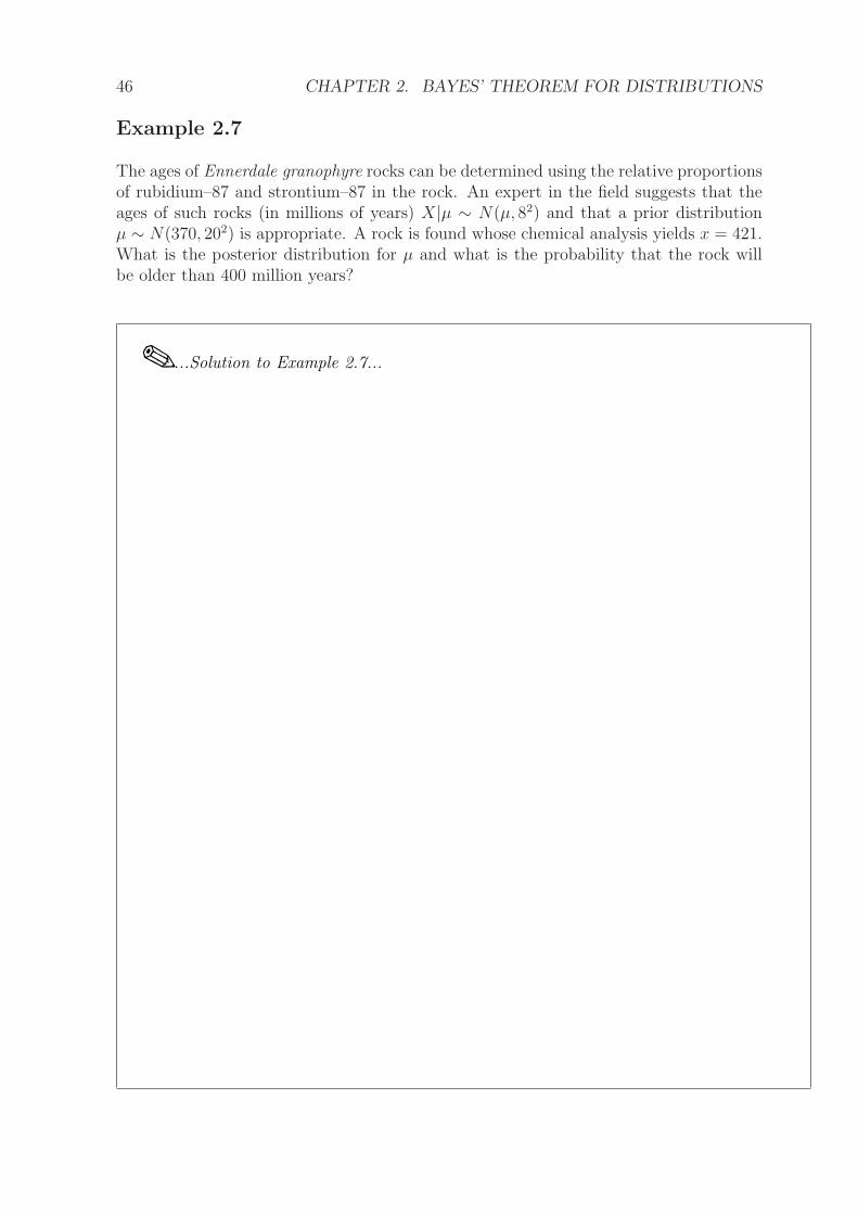
This highlights the benefit of taking the chemical measurements. Note that the largedifference between these probabilities is not necessarily due to the expert’s prior distri-bution being inaccurate, per se, it is probably due to the large prior uncertainty aboutrock ages, as shown in Figure 2.10.

300 350 400 450

0.00

0.01

0.02

0.03

0.04

0.05

µ

dens

ity

Figure 2.10: Prior (dashed) and posterior (solid) densities for the age of the rock

2.3 Posterior distributions and sufficient statistics

We have already met the concept of minimal sufficient statistics. Not surprisingly theyalso play a role in Bayesian Inference.

Suppose that we have data X = (X1, X2, . . . , Xn)T available and we want to make

inferences about the parameters θ in the statistical model f(x|θ). If T is a minimalsufficient statistic then by the Factorisation Theorem

f(x|θ) = h(x) g(t, θ)

for some functions h and g. Therefore, using Bayes Theorem

π(θ|x) ∝ π(θ) f(x|θ)∝ π(θ)h(x) g(t, θ)

∝ π(θ) g(t, θ).

Now it can be shown that, up to a constant not depending on θ, g(t, θ) is equal to theprobability (density) function of T , that is,

g(t, θ) ∝ fT (t|θ).


Hence

π(θ|x) ∝ π(θ) fT (t|θ).

However, applying Bayes Theorem to the data t gives

π(θ|t) ∝ π(θ) fT (t|θ)

and so, since π(θ|x) ∝ π(θ|t) and both are probability (density) functions, we have

π(θ|x) = π(θ|t).

Therefore, our (posterior) beliefs about θ having observed the full data x are the sameas if we had observed only the sufficient statistic T . This is what we would expect if allthe information about θ in the data were contained in the sufficient statistic.

Example 2.8

Suppose we have a random sample from an exponential distribution with a gamma priordistribution, that is, Xi|θ ∼ Exp(θ), i = 1, 2, . . . , n (independent) and θ ∼ Ga(g, h).Determine a sufficient statistic T for θ and verify that π(θ|x) = π(θ|t).

Solution

✎...Solution to Example 2.8...The density of the data is

fX(x|θ) =n∏

i=1

θe−θxi

= θn exp

(

−θn∑

i=1

xi

)

= 1× θn exp

(

−θn∑

i=1

xi

)

= h(x) g(Σxi, θ)

and therefore, by the Factorisation Theorem, T =∑n

i=1Xi is sufficient for θ. NowT |θ ∼ Ga(n, θ) and so

L(θ|t) = fT (t|θ) =θntn−1e−θt

Γ(n), θ > 0.

Also

π(θ) =hg θg−1e−hθ

Γ(g), θ > 0.

2.3. POSTERIOR DISTRIBUTIONS AND SUFFICIENT STATISTICS 49

Solution

✎...Solution to Example 2.8 continued...Therefore, by Bayes Theorem

π(θ|t) ∝ π(θ)L(θ|t)

∝ hg θg−1e−hθ

Γ(g)× θntn−1e−θt

Γ(n), θ > 0

∝ θg+n−1e−(h+t)θ, θ > 0

and so the posterior distribution is θ|t ∼ Ga(g + n, h+ t). This is the same as the resultwe obtained previously for θ|x.


Example 2.9

Suppose we have a random sample from a normal distribution with known varianceand a normal prior distribution for the mean parameter, that is, Xi|µ ∼ N(µ, 1/τ),i = 1, 2, . . . , n (independent) and µ ∼ N(b, 1/d). Determine a sufficient statistic T for µand verify that π(µ|x) = π(µ|t).

Solution

✎...Solution to Example 2.9...Recall from (2.20) that

fX(x|µ) =( τ

2π

)n/2

exp{

−nτ2

[

s2 + (x̄− µ)2]

}

=( τ

2π

)n/2

exp

{

−nτs2

2

}

× exp{

−nτ2(x̄− µ)2

}

= h(x) g(x̄, µ)

and therefore, by the Factorisation Theorem, T = X̄ is sufficient for µ. Now T |µ ∼N(µ, 1/(nτ)) and so

L(µ|t) = fT (t|µ) =(nτ

2π

)1/2

exp{

−nτ2(t− µ)2

}

.

Also

π(µ) =

(

d

2π

)1/2

exp

{

−d2(µ− b)2

}

.

Therefore, by Bayes Theorem

π(µ|t) ∝ π(µ)L(µ|t)

∝(

d

2π

)1/2

exp

{

−d2(µ− b)2

}

×(nτ

2π

)1/2

exp{

−nτ2(t− µ)2

}

∝ exp

{

−d2(µ− b)2 − nτ

2(t− µ)2

}

...

∝ exp

{

−D2(µ−B)2

}

where B and D are as in (2.21), with t replacing x̄; that is, µ|t ∼ N(B, 1/D), the samedistribution as µ|x.

Documents

Chapter 2 Bayes’ Theorem for Distributionsnlf8/teaching/mas2317/notes/chapter2.pdf · Chapter 2 Bayes’ Theorem for Distributions 2.1 Introduction Suppose we have data xwhich we