Magnetostatics

Chapter 4

Part 2

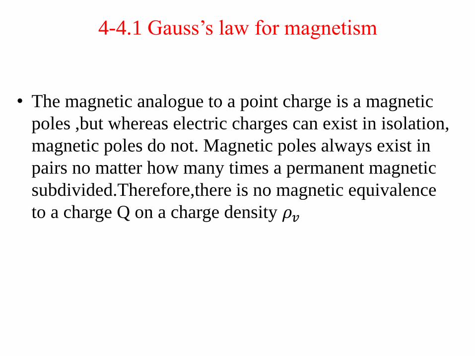
4-4.1 Gauss’s law for magnetism

• The magnetic analogue to a point charge is a magnetic

poles ,but whereas electric charges can exist in isolation,

magnetic poles do not. Magnetic poles always exist in

pairs no matter how many times a permanent magnetic

subdivided.Therefore,there is no magnetic equivalence

to a charge Q on a charge density 𝜌𝑣

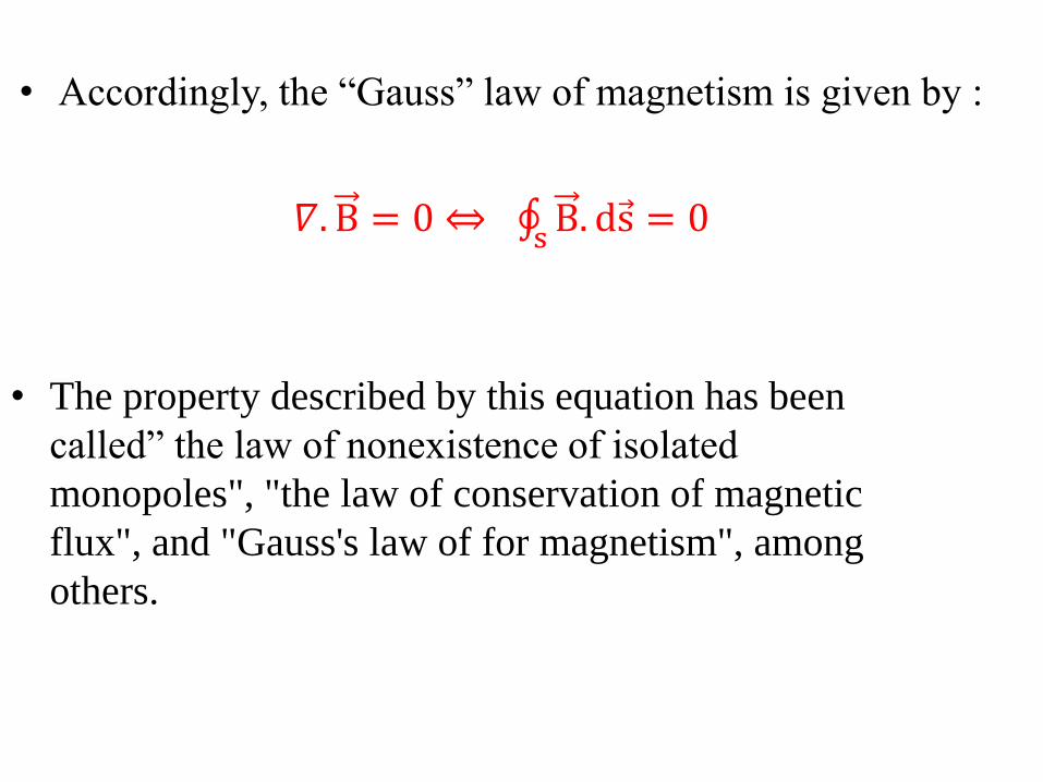
• Accordingly, the “Gauss” law of magnetism is given by :

𝛻. B = 0 ⇔ B. ds s= 0

• The property described by this equation has been

called” the law of nonexistence of isolated

monopoles", "the law of conservation of magnetic

flux", and "Gauss's law of for magnetism", among

others.

• For the electric field lines of the electric dipole, the electric flux through a closed surface surrounding one of the charges is not zero.

• In contrast, magnetic field lines always form continuous closed loops. Therefore the net magnetic flux through the closed surface surrounding the south poles of the magnet(or through any other closed surface)is always zero regardless of the shape of the surface.

4-4.2 Ampere's law

• Ampere’s law is obtained by integrating both sides of

the second of Maxwell's pair for magnetostatic

conditions(steady currents) 𝛻 × 𝐻 = 𝐽

over an open surface S,

(𝛻 × 𝐻𝑠

). 𝑑𝑠 = 𝐽.𝑠

𝑑𝑠

• Using stock’s theorem,

𝛻 × 𝐻 . 𝑑𝑠 = 𝐻. 𝑑𝑙 𝑐𝑠 ,

𝐻. 𝑑𝑙 𝑐= 𝐼 (Ampere′s law)

,where C is the contour bounding the surface S

And 𝐼 = 𝐽 . 𝑑𝑠 is the total current flowing through S.

• The sign convention for the direction of C is

taken so that I and H satisfy the right-hand

rule. If the direction of the thumb points in the

direction of the current I then the direction of

the contour C is along the direction of the

other four fingers.

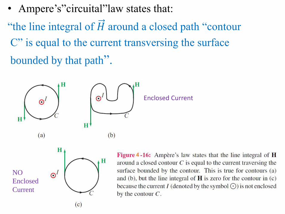
• Ampere’s”circuital”law states that:

“the line integral of 𝐻 around a closed path “contour

C” is equal to the current transversing the surface

bounded by that path”.

NO

Enclosed

Current

Enclosed Current

• The magnetic moment of 𝑚 of a loop of area A

has a magnitude m = 𝐼𝐴, and the direction of

𝑚 is normal to the plane of the loop according

to the right-hand rule.

4-6.1 Orbital and spin Magnetic Moments

• Magnetization in a material substance is associated with atomic currents loops generated by two principal mechanisms:

1- Orbital motions of the electrons around the nucleus and similar motions of the protons around each other in the nucleus.

2- Electron spin.

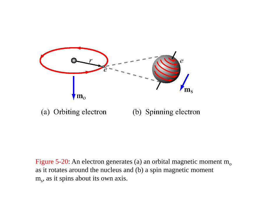
Figure 5-20: An electron generates (a) an orbital magnetic moment mo

as it rotates around the nucleus and (b) a spin magnetic moment

ms, as it spins about its own axis.

• The magnetic moment of an electron is due to the

combination of its orbital motion and its spinning

motion about its own axis.

• The magnetic moment of the nucleus is much smaller

than that of an electron, and therefore the total magnetic

moment of an atom dominated by the sum of the

magnetic moments of its electrons.

• The magnetic behavior of a material is governed

by the interaction of the magnetic dipole moments

of its atoms with an external magnetic field.

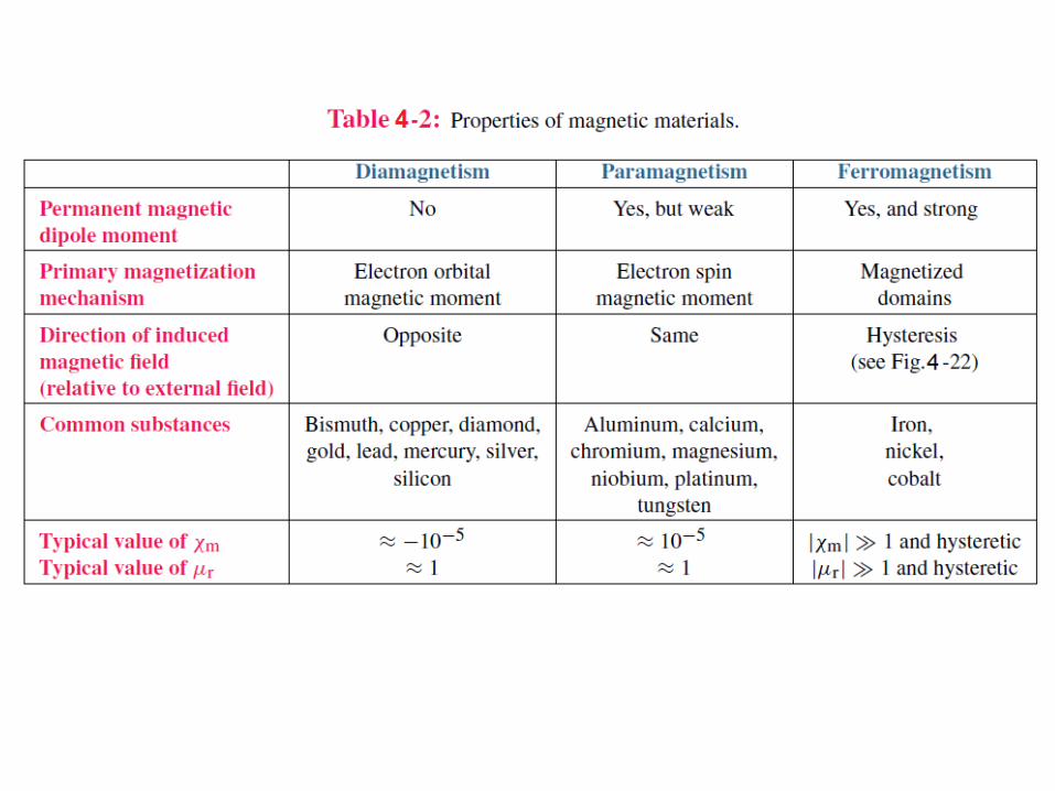
• Accordingly, materials are classified as

“diamagnetic”, “paramagnetic", or

“ferromagnetic”.

• The atoms of a diamagnetic material have no

permanent magnetic dipole moments.

• In contrast, both paramagnetic and

ferromagnetic materials have atoms with

permanent magnetic dipole moments.

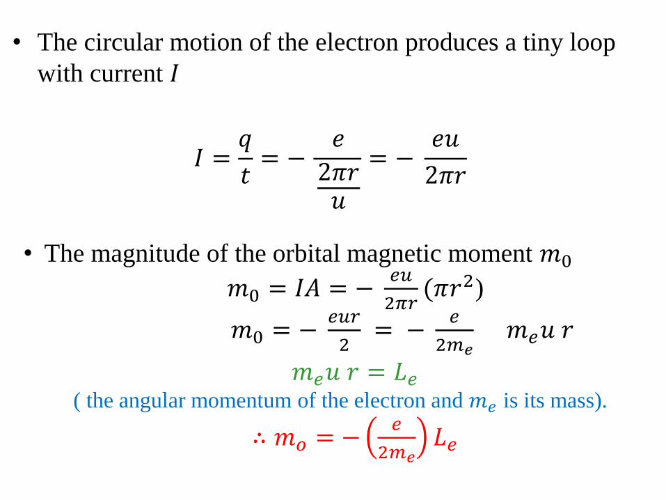
• The circular motion of the electron produces a tiny loop

with current 𝐼

𝐼 =𝑞

𝑡= −

𝑒

2𝜋𝑟𝑢

= − 𝑒𝑢

2𝜋𝑟

• The magnitude of the orbital magnetic moment 𝑚0

𝑚0 = 𝐼𝐴 = − 𝑒𝑢

2𝜋𝑟(𝜋𝑟2)

𝑚0 = − 𝑒𝑢𝑟

2 = −

𝑒

2𝑚𝑒 𝑚𝑒𝑢 𝑟

𝑚𝑒𝑢 𝑟 = 𝐿𝑒 ( the angular momentum of the electron and 𝑚𝑒 is its mass).

∴ 𝑚𝑜 = −𝑒

2𝑚𝑒𝐿𝑒

• 𝐿𝑒is some integer multiple of ℏ =ℎ

2𝜋

(h:plank's constant).

Thus : 𝐿𝑒 = 0, ℏ, 2ℏ, … . .

• The smallest nonzero magnitude of the orbital

magnetic moment of an electron is

𝑚𝑜 = −𝑒ℏ

2𝑚𝑒

• In the absence of an external magnetic field, the

atoms of most materials are oriented randomly, as a

result of which the net magnetic moment generated

by their electrons is either zero or very small.

• The electron also generates a spin magnetic

moment 𝑚𝑠,due to its spinning motion about

its own axis.

• The magnitude of 𝑚𝑠 predicted by quantum

theory is :

𝑚𝑠 = −𝑒ℏ

2𝑚𝑒

4-6.2 Magnetic permeability

• The magnetic flux density 𝐵𝑚 ,

𝐵𝑚 = 𝜇0𝑀

,where 𝑀 is the vector sum of the magnetic dipole

moments of the atoms contained in a unit volume of

the material.

• In the presence of an externally applied magnetic

field 𝐻 , the total flux

𝐵 = 𝜇0𝐻 + 𝜇0𝑀 = 𝜇0(𝐻 +𝑀)

• Generally, the material becomes magnetized in

response to the external field 𝐻.Hence,𝑀 is

expressed as :

𝑀 = 𝑋𝑚𝐻 ,where 𝑋𝑚 is a dimensionless quantity

called "magnetic susceptibility” of the material.

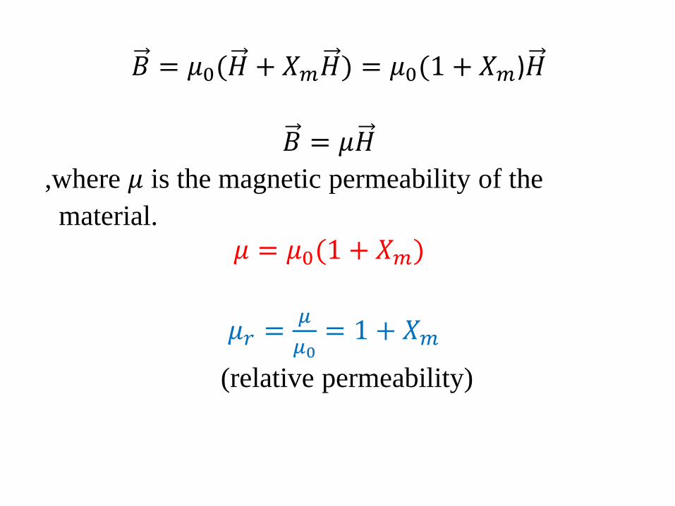
𝐵 = 𝜇0(𝐻 + 𝑋𝑚𝐻) = 𝜇0(1 + 𝑋𝑚)𝐻

𝐵 = 𝜇𝐻

,where 𝜇 is the magnetic permeability of the

material.

𝜇 = 𝜇0(1 + 𝑋𝑚)

𝜇𝑟 =𝜇

𝜇0= 1 + 𝑋𝑚

(relative permeability)

4-6.3 Magnetic Hysteresis of Ferromagnetic Material

• The magnetization behavior of a ferromagnetic

material is described in terms of its B-H

magnetization Curve, where H is the amplitude

of the externally applied magnetic field,𝐻,and

B is the amplitude of the total magnetic flux

density, 𝐵, present within the material.

→

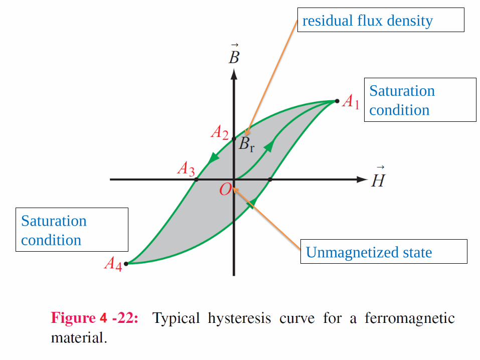
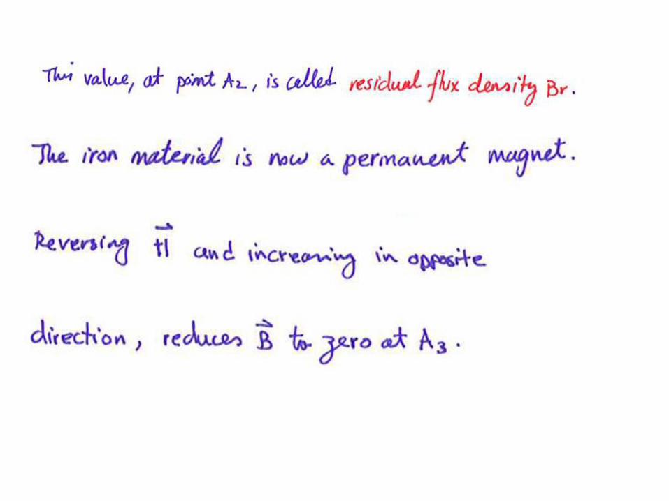
residual flux density

Saturation

condition

Saturation

condition Unmagnetized state

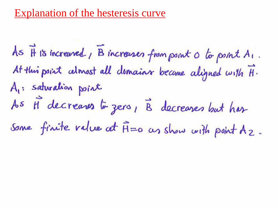
Explanation of the hesteresis curve

• The hysteresis loop shows that the

magnetization process in ferromagnetic

materials depends not only on the external

magnetic field 𝐻,but on the magnetic history

of the material as well.

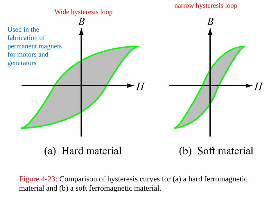
Figure 4-23: Comparison of hysteresis curves for (a) a hard ferromagnetic

material and (b) a soft ferromagnetic material.

Wide hysteresis loop narrow hysteresis loop

Used in the

fabrication of

permanent magnets

for motors and

generators

4-8 Inductance

• An inductor can store magnetic energy in the volume

comparising the inductors.

• It consists of a coil which consists of multiple turns of

wire wound in a helical shape around a cylindrical

core.

• such a structure is called a “solenoid”.

• The core may be air filled or may contain a magnetic

material with magnetic permeability 𝜇.

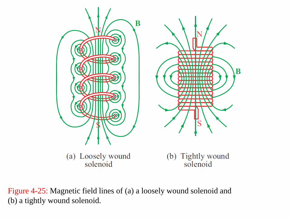
Figure 4-25: Magnetic field lines of (a) a loosely wound solenoid and

(b) a tightly wound solenoid.

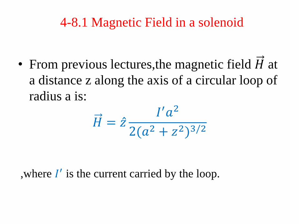
4-8.1 Magnetic Field in a solenoid

• From previous lectures,the magnetic field 𝐻 at

a distance z along the axis of a circular loop of

radius a is:

𝐻 = 𝑧 𝐼′𝑎2

2(𝑎2 + 𝑧2)3/2

,where 𝐼′ is the current carried by the loop.

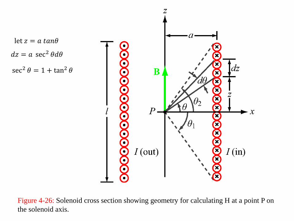
Figure 4-26: Solenoid cross section showing geometry for calculating H at a point P on

the solenoid axis.

let 𝑧 = 𝑎 𝑡𝑎𝑛𝜃

𝑑𝑧 = 𝑎 sec2 𝜃𝑑𝜃

sec2 𝜃 = 1 + tan2 𝜃

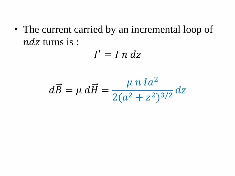
• The current carried by an incremental loop of

𝑛𝑑𝑧 turns is :

𝐼′ = 𝐼 𝑛 𝑑𝑧

𝑑𝐵 = 𝜇 𝑑𝐻 =𝜇 𝑛 𝐼𝑎2

2(𝑎2 + 𝑧2)3/2𝑑𝑧

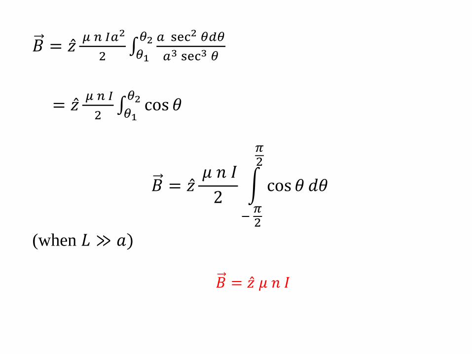
𝐵 = 𝑧 𝜇 𝑛 𝐼𝑎2

2

𝑎 sec2 𝜃𝑑𝜃

𝑎3 sec3 𝜃

𝜃2𝜃1

= 𝑧 𝜇 𝑛 𝐼

2 cos 𝜃𝜃2𝜃1

𝐵 = 𝑧 𝜇 𝑛 𝐼

2 cos 𝜃

𝜋2

− 𝜋2

𝑑𝜃

(when 𝐿 ≫ 𝑎)

𝐵 = 𝑧 𝜇 𝑛 𝐼

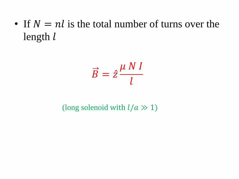
• If 𝑁 = 𝑛𝑙 is the total number of turns over the

length 𝑙

𝐵 = 𝑧 𝜇 𝑁 𝐼

𝑙

(long solenoid with 𝑙/𝑎 ≫ 1)

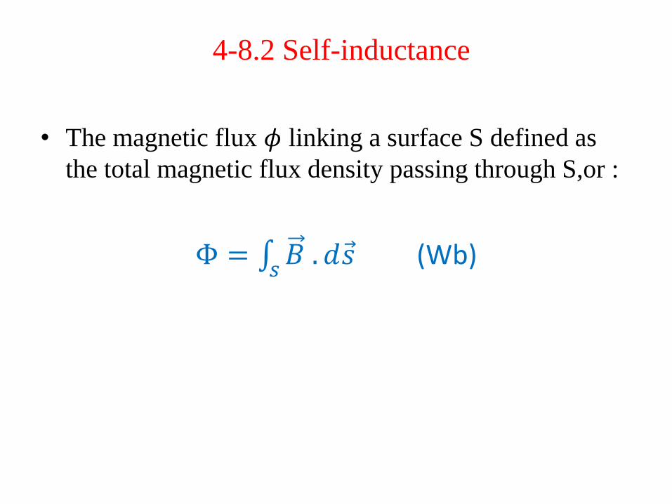
• The magnetic flux 𝜙 linking a surface S defined as

the total magnetic flux density passing through S,or :

Φ = 𝐵 . 𝑑𝑠 𝑠 (Wb)

4-8.2 Self-inductance

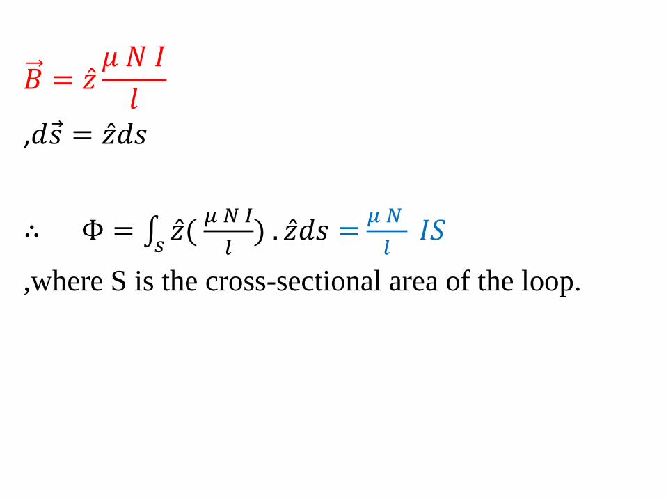
𝐵 = 𝑧 𝜇 𝑁 𝐼

𝑙

,𝑑𝑠 = 𝑧 𝑑𝑠

∴ Φ = 𝑧 ( 𝜇 𝑁 𝐼

𝑙𝑠) . 𝑧 𝑑𝑠 =

𝜇 𝑁

𝑙 𝐼𝑆

,where S is the cross-sectional area of the loop.

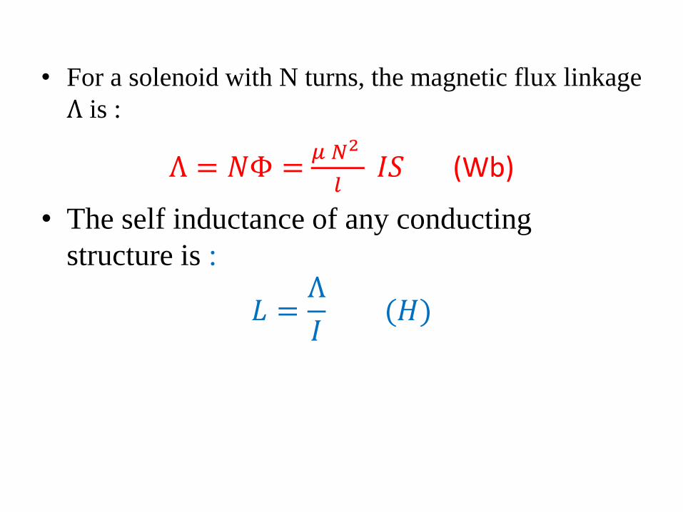
• For a solenoid with N turns, the magnetic flux linkage

Λ is :

Λ = 𝑁Φ = 𝜇 𝑁2

𝑙 𝐼𝑆 (Wb)

• The self inductance of any conducting

structure is :

𝐿 =Λ

𝐼 (𝐻)

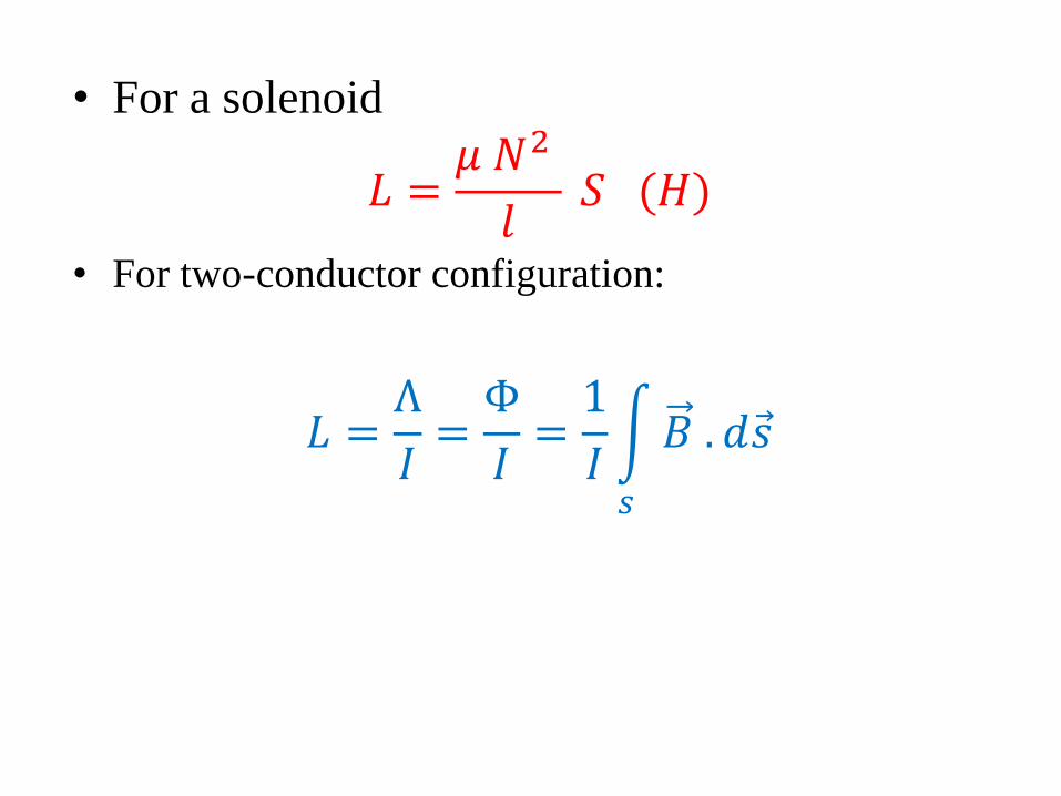
• For a solenoid

𝐿 =𝜇 𝑁2

𝑙 𝑆 (𝐻)

• For two-conductor configuration:

𝐿 =Λ

𝐼=Φ

𝐼=1

𝐼 𝐵 . 𝑑𝑠

𝑠

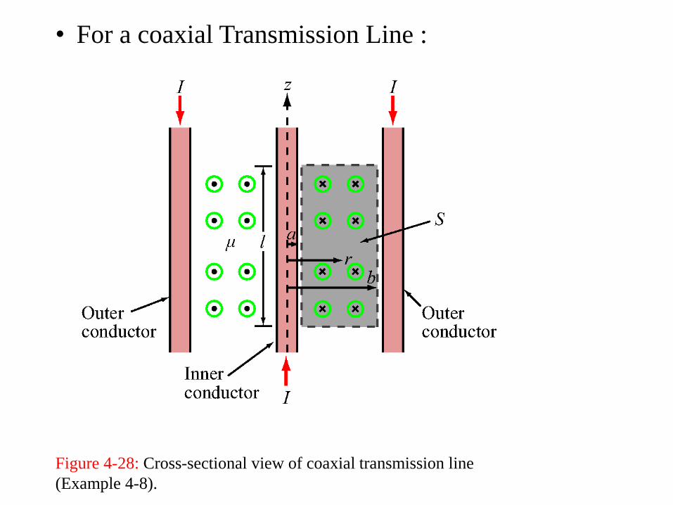
• For a coaxial Transmission Line :

Figure 4-28: Cross-sectional view of coaxial transmission line

(Example 4-8).

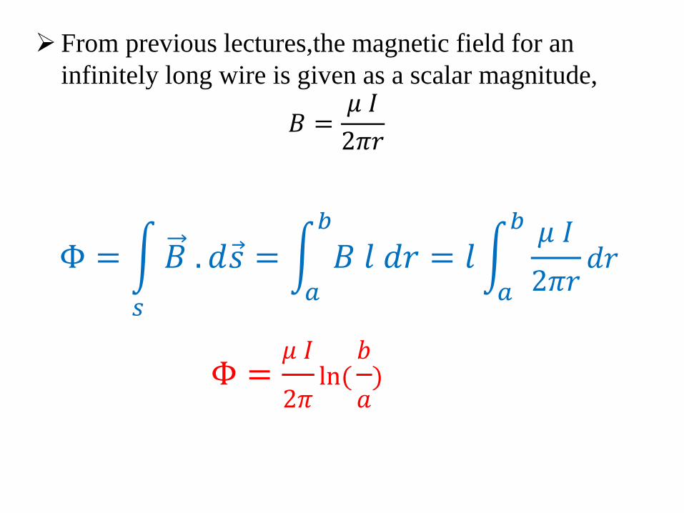
From previous lectures,the magnetic field for an

infinitely long wire is given as a scalar magnitude,

𝐵 =𝜇 𝐼

2𝜋𝑟

Φ = 𝐵 . 𝑑𝑠

𝑠

= 𝐵 𝑙 𝑑𝑟𝑏

𝑎

= 𝑙 𝜇 𝐼

2𝜋𝑟𝑑𝑟

𝑏

𝑎

Φ =𝜇 𝐼

2𝜋ln(𝑏

𝑎)

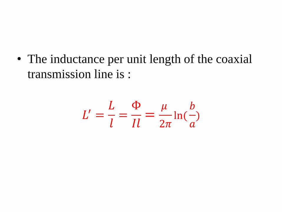
• The inductance per unit length of the coaxial

transmission line is :

𝐿′ =𝐿

𝑙=Φ

𝐼𝑙=𝜇

2𝜋ln(𝑏

𝑎)