Embed Size (px)
Citation preview
���������������� ������
Faculty of Engineering and Science (FES) Department of Chemical Engineering
�
���������
���� �������������
������������
����� �
�
�
�����������
� ����������������������������������������������������������������
�� ��� ���!�"��#��"���������� �������������������������������������������������������
$� % ����� &���'�� ��� �����������������������������������������������������
(� )�*�����+�� ���������������������������������������������������������������������������
,� !�"��#�'�--��� �% �--����� �����������������������������������������������������
.� /����'������� �% ���� �������������������������������������������������������
0� !�"��#�!�"��#������� �����������������������������������������������������������
1� ���2�'�2��� ���������������������������������������������������������������������������������
3� ����#�4����������������������������������������������������������������������������������
5� ����#���#�/�#����������������������������������������������������������������������������
����������� ������� ���� ����������������
��
Table of Content
1.0 UNIT OBJECTIVES.............................................................................................................3
2.0 UNIT OUTCOMES...............................................................................................................3
3.0 SUBJECT SYNOPSIS...........................................................................................................3
4.0 LABORATORY SAFETY, RULES AND REGULATIONS ............................................4
4.1 General Rules...............................................................................................................4
4.2 Laboratory Safety Rules ..............................................................................................5
5.0 RESPONSIBILITY OF STUDENTS...................................................................................6
6.0 ASSESSMENTS.....................................................................................................................7
6.1 Overall Performance in Laboratory during Experiment Session (10 marks) ..............7
6.2 Laboratory Reports (10 marks)....................................................................................8
7.0 LABORATORY REPORT WRITING ...............................................................................9
7.1 Content.........................................................................................................................9
7.2 Specification ..............................................................................................................11
7.3 Formatting..................................................................................................................12
Appendix A: Material Safety Data Sheet (MSDS)..................................................................... 114
����������� ������� ���� ����������������
��
1.0 UNIT OBJECTIVES
This subject will help the students to develop their skills of collecting, analysing and presenting the results of data acquired within a well-defined experimental system. The specific objectives are to:
� combine elements of theory and practice particularly in thermodynamics, heat and mass transfer, fluid mechanics and fluid separation
� develop competence in conducting experimental work
� acquire a "hands-on" laboratory experience
� familiarise with laboratory safety procedures
� develop and demonstrate a knowledge of experimental error analysis, probability and statistics
� work collaboratively within a group setting
� develop skills in handling, manipulating and maintaining basic engineering machinery
� develop practical skills to plan and design laboratory experiments
2.0 UNIT OUTCOMES
On completion of this unit, a student should be able to:
� collect and analyse experimental data and its relationship to theoretical principles of
� fluid mechanics
� heat and mass transfer
� thermodynamics
� fluid separation
� prepare a written laboratory reports that clearly present the experimental results, analysis, and relationship to theory
� develop skills in operating common chemical engineering equipment and measurement apparatus
3.0 SUBJECT SYNOPSIS
A laboratory course in pilot-scale processes involving thermodynamics, heat and mass transfer and fluid mechanics. Students will acquire the skills in project definition, experimental operation, analytical procedures, data analysis and technical reports preparation.
����������� ������� ���� ����������������
��
4.0 LABORATORY SAFETY, RULES AND REGULATIONS
Laboratory safety is the top priority and this requires all people in the laboratory to be observing safe practices at all times!
4.1 General Rules
� Students must abide the dress code while working in the laboratory.
� Laboratory coat must be worn all the time when working in the laboratory.
� Only closed toe shoes are allowed in the laboratory. Do not wear sandals, slippers and high heel shoes inside the laboratory.
� Students with long hair must get their hair tied up tidily when doing laboratory work.
� Bags and other belongings must be kept at the designated places.
� Foods, drinks and smoking are strictly prohibited inside the laboratory.
� Noise must be kept to the minimum as a courtesy to respect others.
� Students are not allowed to work alone without the supervision of laboratory instructor/officer. There must be at least 2 persons present in the laboratory at same time.
� Students are not allowed to bring any outsiders (non-registered parties) into the laboratory.
� Any unauthorized experiment without the knowledge of laboratory instructor is prohibited.
� All instrument and equipment must be handled with care.
� Workspace has to be cleaned and tidied up after the experiment completed. Instrument and equipment must be returned orderly after use.
� Students are strictly prohibited to take any equipment or any technical manuals out from the laboratory without the permission of laboratory instructor/officer.
� Students are required to instil an instinctive awareness towards property value of laboratory equipment and to be responsible when using it. Any damages can cause to jeopardise the success of not only the individual work but also to the university.
� Do not attempt to remove and dismantle any parts of the equipment from its original design without permission.
� Students shall be liable for damages of equipment caused by individual negligence. If damages occurred, an investigation will take place to identify the causes and the names of the involved students will be recorded for faculty attention.
� Please check the notice board regularly and pay attention to laboratory announcements.
� Disciplinary action shall be taken against those students who are failed to abide the rules and regulations.

����������� ������� ���� ����������������
��
4.2 Laboratory Safety Rules
� It is always a good practice and the responsibility of an individual to keep a tidy working condition in laboratory.
� It is important for each student to follow the procedures given by the laboratory instructor when conducting laboratory experiment.
� Before any experiment starts, students must study the information / precaution steps and understand the procedures mentioned in the given laboratory sheet.
� Students should report immediately to laboratory instructor/officer if the laboratory equipment is suspected to be malfunctioning or faulty.
� Student should report immediately to the laboratory instructor/officer if discovered any damages on equipment or any hazardous situation.
� Students should report immediately to the laboratory instructor/officer if any injury occurred.
� If there is a tingling feel when working with electrical devices, stop and switch off the devices immediately. Place a warning note before reporting to the laboratory instructor/officer and wait for further instruction.
� Do not work with electricity under wet condition in laboratory. Electric shock is a serious fatal error due to human negligence and may cause death.
� Students are required to wear goggles, gloves, apron and mask when handling corrosive or active chemical agents.
� Hazardous chemical agents must be properly stored and labelled in a designated place. Students must acquire and study the material safety data sheet of a particular chemical agent before using it.
(Extracted from Student Laboratory Guidelines. Refer to the Guidelines for complete rules & regulations)

����������� ������� ���� ����������������
��
5.0 RESPONSIBILITY OF STUDENTS
� Attendance is compulsory. Attendance shall be taken during the laboratory session.
� Please sign your attendance when you attend the laboratory session.
� Laboratory report can only be accepted for submission if the student has attended the laboratory session.
� Student must be punctual to attend laboratory session.
� Students who are late for more than 30 minutes will be barred from attending the laboratory session. Only students with valid reason of medical basis or unforeseen circumstances can be considered to apply for laboratory replacement.
� Students are expected to study the lab sheet before the laboratory session start.
� Student must understand all the safety measures / precaution steps before starting any experiments.
� Student must complete the experiment within the allocated duration of laboratory session.
� Students are responsible for the condition of their working area at the end of each laboratory session. All power to the equipment and instruments should be turned off, and cooling water flows should be shut off. Glassware used should be cleaned and dried.
� Students have to pass up their experiment result to laboratory officer on the same day after every experiment. A copy of the experimental result (with chop) must be attached together with the laboratory report.
� Fabricating results and plagiarism are strictly prohibited. Strict action will be taken if student is found fabricating results or copy from others.
� Students have to pass up their laboratory report 2 weeks after the date of experiment to laboratory officer.

����������� ������� ���� ����������������
��
6.0 ASSESSMENTS
6.1 Overall Performance in Laboratory during Experiment Session (10 marks)
This is a group assessment. Each student performance in the laboratory during the experiment session will be observed and marks will be given to the group as a whole.
The performance will be assessed based on the following criteria:
Criteria Description Marks
Safety Awareness
� Adhere to laboratory safety, rules and regulation. � Abide to dress code (lab coat, shoes, long pants etc.)
while working in the laboratory. � Understand all the safety measures / precaution steps
before starting any experiments. � Proper safety equipment such as goggles, gloves etc.
were used when necessary. � Show precautions when handling chemicals.
Punctuality � Attend laboratory session on time.
Preparation � Show understanding in the experiment that are about to carry out.
Cleanliness and Responsibility
� Workspace is clean and tidied up after the experiment completed.
� Instrument and equipment are returned orderly after use.
� Show instinctive awareness towards property value of laboratory equipment and instruments and their responsibility in handling them.
10

����������� ������� ���� ����������������
��
6.2 Laboratory Reports (10 marks)
Laboratory report will be assessed based on the following criteria:
Criteria Description Marks
Overall Presentation of Report
� Organisation of report with the correct format and necessary information such as titles, figure explanations.
� Report is written in clear and concise English.
2.5
Observations / Data / Result Presentation
� Valid observations, consistent with event and demonstrate attention to detail.
� Data are presented in an organised manner. � Quality of data reflects student’s ability to perform
experiment successfully and utilise computer software in analysis (if applicable).
� All calculations and graphs are correct.
2.5
Discussion � Discussion shows complete understanding of experiment and the significance of data.
� Logical explanation for problems in the data.
3.5
Conclusion � Summary of key findings in a clear statement. � Clearly show relationships between data and
conclusion. � Express views on the weakness of the experimental
design (if there is any), or what is the implication of the conclusion.
1.5
TOTAL 10
����������� ������� ���� ����������������
��
7.0 LABORATORY REPORT WRITING
Laboratory reports are the most frequent document written by an engineering student. A laboratory report should not be used to merely record the expected and observed results but demonstrate the writer’s comprehension of the concept behind the data. A good laboratory report should address the following questions:
� “Why?” – Why did I do this particular experiment?
� “How?” – How did I actually carry it out?
� “What?” – What did I find? What were my results?
� “So What?” – What does my result mean? What is the significance of the result? What are my conclusions?
��������������������������� ���!�
"#�$%& �'����%���('#('�)��'#�
$�& & %'($�������(��)(�'(�($�'$�*�
The laboratory report should be written with the same professionalism that would be used to present the results of a major industrial project. A good report of technical work quantitatively states significant results of experiments and computations and explains how they were obtained, what they mean, and how they are useful. The report should be clear, concise, and accurate.
7.1 Content
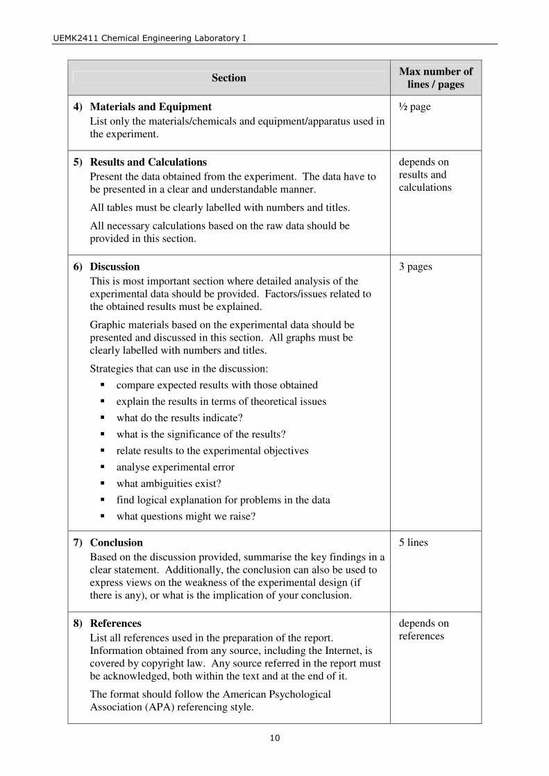
The laboratory report should follow the following format and all the pages should be numbered except the cover page.
Section Max number of lines / pages
UTAR Laboratory Cover Page
1) Title of Experiment 1 – 2 lines
2) Objectives of Experiment 1 – 5 lines
3) Introduction Provide a scientific background related to the experiment and provides the reader with justification for why the work was carried out.
½ page
����������� ������� ���� ����������������
� �
Section Max number of lines / pages
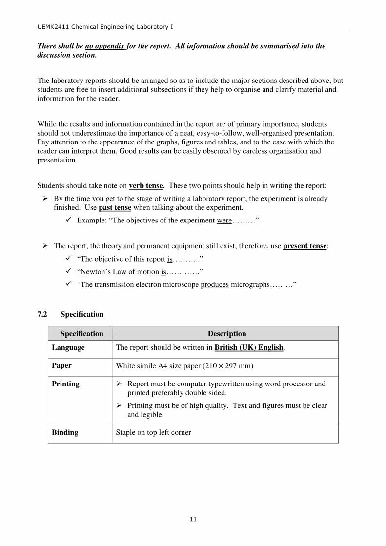
4) Materials and Equipment List only the materials/chemicals and equipment/apparatus used in the experiment.
½ page
5) Results and Calculations Present the data obtained from the experiment. The data have to be presented in a clear and understandable manner.
All tables must be clearly labelled with numbers and titles.
All necessary calculations based on the raw data should be provided in this section.
depends on results and calculations
6) Discussion This is most important section where detailed analysis of the experimental data should be provided. Factors/issues related to the obtained results must be explained.
Graphic materials based on the experimental data should be presented and discussed in this section. All graphs must be clearly labelled with numbers and titles.
Strategies that can use in the discussion: � compare expected results with those obtained � explain the results in terms of theoretical issues � what do the results indicate? � what is the significance of the results? � relate results to the experimental objectives � analyse experimental error � what ambiguities exist? � find logical explanation for problems in the data � what questions might we raise?
3 pages
7) Conclusion Based on the discussion provided, summarise the key findings in a clear statement. Additionally, the conclusion can also be used to express views on the weakness of the experimental design (if there is any), or what is the implication of your conclusion.
5 lines
8) References List all references used in the preparation of the report. Information obtained from any source, including the Internet, is covered by copyright law. Any source referred in the report must be acknowledged, both within the text and at the end of it.
The format should follow the American Psychological Association (APA) referencing style.
depends on references
����������� ������� ���� ����������������
���
There shall be no appendix for the report. All information should be summarised into the discussion section.
The laboratory reports should be arranged so as to include the major sections described above, but students are free to insert additional subsections if they help to organise and clarify material and information for the reader.
While the results and information contained in the report are of primary importance, students should not underestimate the importance of a neat, easy-to-follow, well-organised presentation. Pay attention to the appearance of the graphs, figures and tables, and to the ease with which the reader can interpret them. Good results can be easily obscured by careless organisation and presentation.
Students should take note on verb tense. These two points should help in writing the report:
� By the time you get to the stage of writing a laboratory report, the experiment is already finished. Use past tense when talking about the experiment.
� Example: “The objectives of the experiment were………”
� The report, the theory and permanent equipment still exist; therefore, use present tense:
� “The objective of this report is………..”
� “Newton’s Law of motion is………….”
� “The transmission electron microscope produces micrographs………”
7.2 Specification
Specification Description
Language The report should be written in British (UK) English.
Paper White simile A4 size paper (210 × 297 mm)
Printing � Report must be computer typewritten using word processor and printed preferably double sided.
� Printing must be of high quality. Text and figures must be clear and legible.
Binding Staple on top left corner
����������� ������� ���� ����������������
���
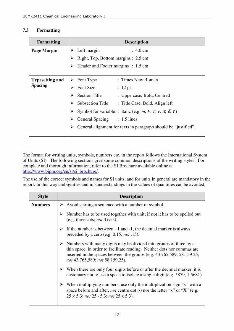
7.3 Formatting
Formatting Description
Page Margin � Left margin : 4.0 cm
� Right, Top, Bottom margins : 2.5 cm
� Header and Footer margins : 1.5 cm
Typesetting and Spacing
� Font Type : Times New Roman
� Font Size : 12 pt
� Section Title : Uppercase, Bold, Centred
� Subsection Title : Title Case, Bold, Align left
� Symbol for variable : Italic (e.g. m, P, T, v, α, δ, τ )
� General Spacing : 1.5 lines
� General alignment for texts in paragraph should be “justified”.
The format for writing units, symbols, numbers etc. in the report follows the International System of Units (SI). The following sections give some common descriptions of the writing styles. For complete and thorough information, refer to the SI Brochure available online at http://www.bipm.org/en/si/si_brochure/.
The use of the correct symbols and names for SI units, and for units in general are mandatory in the report. In this way ambiguities and misunderstandings in the values of quantities can be avoided.
Style Description
Numbers � Avoid starting a sentence with a number or symbol.
� Number has to be used together with unit; if not it has to be spelled out (e.g. three cats; not 3 cats).
� If the number is between +1 and -1, the decimal marker is always preceded by a zero (e.g. 0.15; not .15).
� Numbers with many digits may be divided into groups of three by a thin space, in order to facilitate reading. Neither dots nor commas are inserted in the spaces between the groups (e.g. 43 765 589, 58.159 25; not 43,765,589; not 58.159,25).
� When there are only four digits before or after the decimal marker, it is customary not to use a space to isolate a single digit (e.g. 5879, 1.5681)
� When multiplying numbers, use only the multiplication sign “×” with a space before and after, not centre dot (⋅⋅⋅⋅) nor the letter “x” or “X” (e.g. 25 × 5.3; not 25 ⋅⋅⋅⋅ 5.3; not 25 x 5.3).

����������� ������� ���� ����������������
���
Style Description
Units If possible, use SI units; although other commonly used non-SI units are also acceptable (e.g. °C for temperature, bar for pressure).
Spacing
� One spacing between number and unit (e.g. 5 cm, 50 °C, 30 %; not 5cm; not 50°C; not 30%).
� Exception for angular degree (°), minute (′) and second (″) (e.g. 3°, 45′) which are placed immediately after the number.
Symbols for Units
� Use symbol for units and not their abbreviation (e.g. 5 s; not 5 sec.).
� Symbols for units are written in upright type i.e. not italic (e.g. m for metres, g for grams). This is to differentiate them from italic type symbols used for variables (e.g. m for mass).
� Symbols for units are written in lowercase, except for symbols derived from the name of a person, which start with uppercase. However, the unit name itself is written in lowercase. (e.g. the unit for pressure is named after Blaise Pascal; the unit itself is written as “pascal” whereas the symbol is “Pa”; 5 Pa or 5 pascal; 5 J or 5 joule; 5 N or 5 newton)
� Symbols are not pluralised (e.g. 5 kg; not 5 kgs).
� Symbols do not have an appended period / full stop (.) unless at the end of a sentence.
� Symbols derived from multiple units by multiplication are joined with a space or centre dot (⋅⋅⋅⋅) (e.g. N m for N⋅m). Hyphens (-) should not be used (e.g. not N-m) [Note: centre dot (⋅⋅⋅⋅) is different from period / full stop (.); centre dot is available under command Insert > Symbol].
� Symbols formed by division of two units are joined with a solidus ( ⁄ ) (slash ( / ) is also acceptable) or given as a negative exponent (e.g. m/s or m s-1).
� Only one solidus should be used (e.g. kg⋅m-1⋅s-2 or kg/(m⋅s2); not kg/m/s2).
� Do not mix unit symbols and unit names within one expression (e.g. coulomb per kilogram; not coulomb per kg).
����������� ������� ���� ����������������
���
Style Description
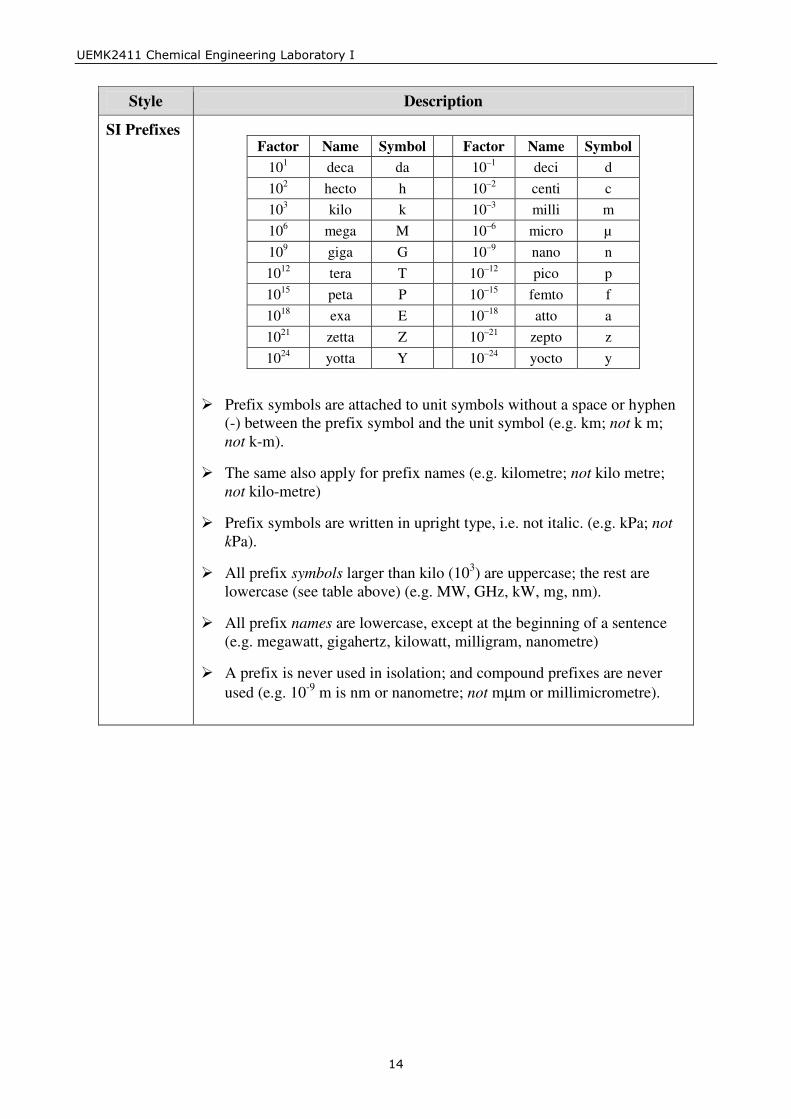
SI Prefixes
Factor Name Symbol Factor Name Symbol 101 deca da 10–1 deci d 102 hecto h 10–2 centi c 103 kilo k 10–3 milli m 106 mega M 10–6 micro µ 109 giga G 10–9 nano n 1012 tera T 10–12 pico p 1015 peta P 10–15 femto f 1018 exa E 10–18 atto a 1021 zetta Z 10–21 zepto z 1024 yotta Y 10–24 yocto y
� Prefix symbols are attached to unit symbols without a space or hyphen (-) between the prefix symbol and the unit symbol (e.g. km; not k m; not k-m).
� The same also apply for prefix names (e.g. kilometre; not kilo metre; not kilo-metre)
� Prefix symbols are written in upright type, i.e. not italic. (e.g. kPa; not kPa).
� All prefix symbols larger than kilo (103) are uppercase; the rest are lowercase (see table above) (e.g. MW, GHz, kW, mg, nm).
� All prefix names are lowercase, except at the beginning of a sentence (e.g. megawatt, gigahertz, kilowatt, milligram, nanometre)
� A prefix is never used in isolation; and compound prefixes are never used (e.g. 10-9 m is nm or nanometre; not mµm or millimicrometre).
����������� ������� ���� ���������������� � �!"�� �������
���
Experiment 1
Heat Exchangers - Shell & Tube, Plate & Frame
1.0 OBJECTIVES OF EXPERIMENT
� To study different types of heat exchanger operation.
� To collect related experimental data for calculation of heat losses, heat transfer coefficient and log mean temperature different.
� To study the effect of flow rate on heat transfer.
� To perform energy balance around a heat exchanger.
� To study temperature profiles across a heat exchanger.
2.0 INTRODUCTION
2.1 Shell & Tube Heat Exchanger
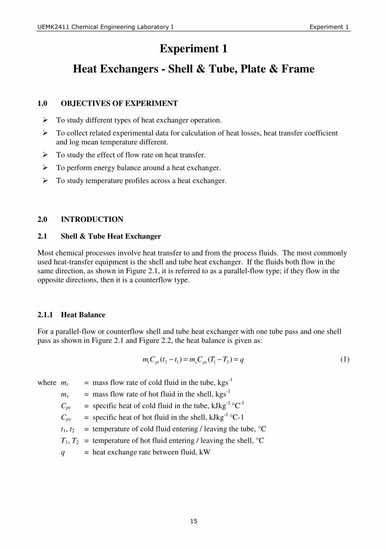
Most chemical processes involve heat transfer to and from the process fluids. The most commonly used heat-transfer equipment is the shell and tube heat exchanger. If the fluids both flow in the same direction, as shown in Figure 2.1, it is referred to as a parallel-flow type; if they flow in the opposite directions, then it is a counterflow type.
2.1.1 Heat Balance
For a parallel-flow or counterflow shell and tube heat exchanger with one tube pass and one shell pass as shown in Figure 2.1 and Figure 2.2, the heat balance is given as: qTTCmttCm pssptt =−=− )()( 2112 (1) where mt = mass flow rate of cold fluid in the tube, kgs-1 ms = mass flow rate of hot fluid in the shell, kgs-1 Cpt = specific heat of cold fluid in the tube, kJkg-1 °C-1 Cps = specific heat of hot fluid in the shell, kJkg-1 °C-1 t1, t2 = temperature of cold fluid entering / leaving the tube, °C T1, T2 = temperature of hot fluid entering / leaving the shell, °C q = heat exchange rate between fluid, kW
����������� ������� ���� ���������������� � �!"�� �������
���
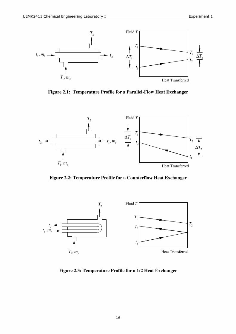
Figure 2.1: Temperature Profile for a Parallel-Flow Heat Exchanger
Figure 2.2: Temperature Profile for a Counterflow Heat Exchanger
Figure 2.3: Temperature Profile for a 1:2 Heat Exchanger
tmt ,1
smT ,1
2t
2T
2t
1T
1t
2T
Fluid T
Heat Transferred
tmt ,1
smT ,1
2t
2T
2t
1T
1t
2T
2T∆
1T∆
Fluid T
Heat Transferred
tmt ,1
smT ,1
2t
2T
1t
1T
2t2T
1T∆ 2T∆
Fluid T
Heat Transferred
����������� ������� ���� ���������������� � �!"�� �������
���
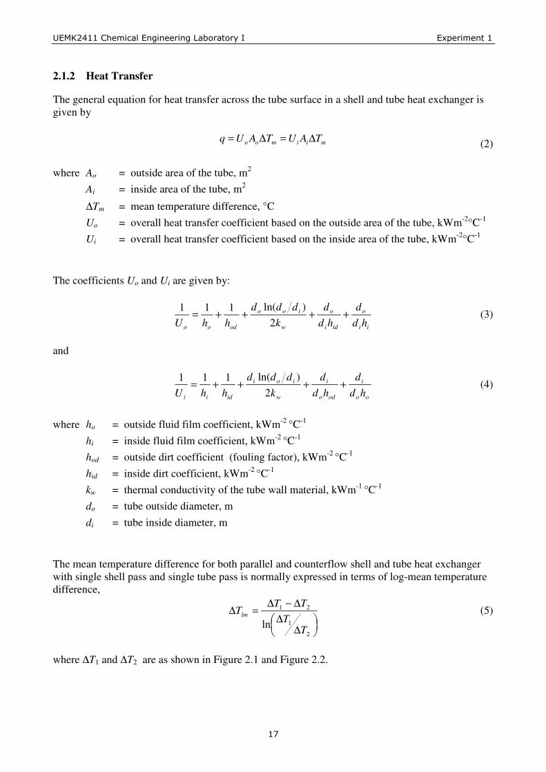
2.1.2 Heat Transfer
The general equation for heat transfer across the tube surface in a shell and tube heat exchanger is given by
miimoo TAUTAUq ∆=∆= (2) where Ao = outside area of the tube, m2 Ai = inside area of the tube, m2
∆Tm = mean temperature difference, °C Uo = overall heat transfer coefficient based on the outside area of the tube, kWm-2°C-1 Ui = overall heat transfer coefficient based on the inside area of the tube, kWm-2°C-1 The coefficients Uo and Ui are given by:
ii
o
idi
o
w
ioo
odoo hdd
hdd
kddd
hhU++++=
2)ln(111
(3)
and
oo
i
odo
i
w
ioi
idii hdd
hdd
kddd
hhU++++=
2)ln(111
(4)
where ho = outside fluid film coefficient, kWm-2 °C-1 hi = inside fluid film coefficient, kWm-2 °C-1 hod = outside dirt coefficient (fouling factor), kWm-2 °C-1 hid = inside dirt coefficient, kWm-2 °C-1 kw = thermal conductivity of the tube wall material, kWm-1 °C-1 do = tube outside diameter, m di = tube inside diameter, m The mean temperature difference for both parallel and counterflow shell and tube heat exchanger with single shell pass and single tube pass is normally expressed in terms of log-mean temperature difference,
���
���
∆∆
∆−∆=∆
2
1
21
ln TT
TTTlm (5)
where ∆T1 and ∆T2 are as shown in Figure 2.1 and Figure 2.2.
����������� ������� ���� ���������������� � �!"�� �������
���
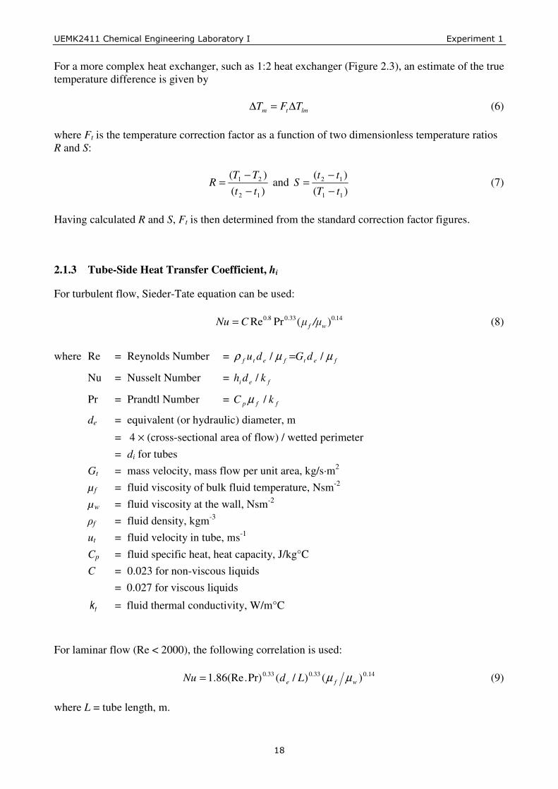
For a more complex heat exchanger, such as 1:2 heat exchanger (Figure 2.3), an estimate of the true temperature difference is given by lmtm TFT ∆=∆ (6) where Ft is the temperature correction factor as a function of two dimensionless temperature ratios R and S:
)()(
12
21
ttTT
R−−
= and )()(
11
12
tTtt
S−−
= (7)
Having calculated R and S, Ft is then determined from the standard correction factor figures.
2.1.3 Tube-Side Heat Transfer Coefficient, hi
For turbulent flow, Sieder-Tate equation can be used: 14033080 )(PrRe .
wf.. /��CNu = (8)
where Re = Reynolds Number = fetfetf dGdu µµρ // =
Nu = Nusselt Number = fei kdh /
Pr = Prandtl Number = ffp kC /µ
de = equivalent (or hydraulic) diameter, m
= 4 × (cross-sectional area of flow) / wetted perimeter = di for tubes Gt = mass velocity, mass flow per unit area, kg/s·m2 µ f = fluid viscosity of bulk fluid temperature, Nsm-2 µw = fluid viscosity at the wall, Nsm-2 �f = fluid density, kgm-3 ut = fluid velocity in tube, ms-1 Cp = fluid specific heat, heat capacity, J/kg°C C = 0.023 for non-viscous liquids = 0.027 for viscous liquids
fk = fluid thermal conductivity, W/m°C
For laminar flow (Re < 2000), the following correlation is used: 14.033.033.0 )()/(Pr).(Re86.1 wfe LdNu µµ= (9) where L = tube length, m.

����������� ������� ���� ���������������� � �!"�� �������
���
2.1.4 Tube-Side Pressure Drop, ∆∆∆∆Pt
The tube-side pressure drop is given by:
[ ]2
5.2))(/(82tfm
wifpt
udLjNP
ρµµ +=∆ − (10)
where ∆Pt = tube-side pressure drop, N/m2 Np = number of tube-side passes jf = tube dimensionless friction factor (Figure C.3 in Appendix C) L = length of one tube, m ut = tube-side velocity, m/s m = 0.25 for laminar, Re < 2100 = 0.14 for turbulent, Re > 2100
2.1.5 Shell-Side Heat Transfer Coefficient, hs (Kern’s Method)
In order to determine the heat transfer coefficient for fluid film in shell, the cross-sectional area of flow As is first calculate for hypothetical row of tubes of the shell as follows: tBsots plDdpA /)( −= (11) where do = tube outside diameter, m pt = tube pitch, m Ds = shell inside diameter, m lB = distance between baffle, m Then, the shell-side mass velocity, Gs and linear velocity, us are calculated as follows: sss AWG = (12) fss Gu ρ= (13) where W s = fluid flow rate on the shell-side, kg/s � f = shell-side fluid density, kg/m3
����������� ������� ���� ���������������� � �!"�� �������
� �
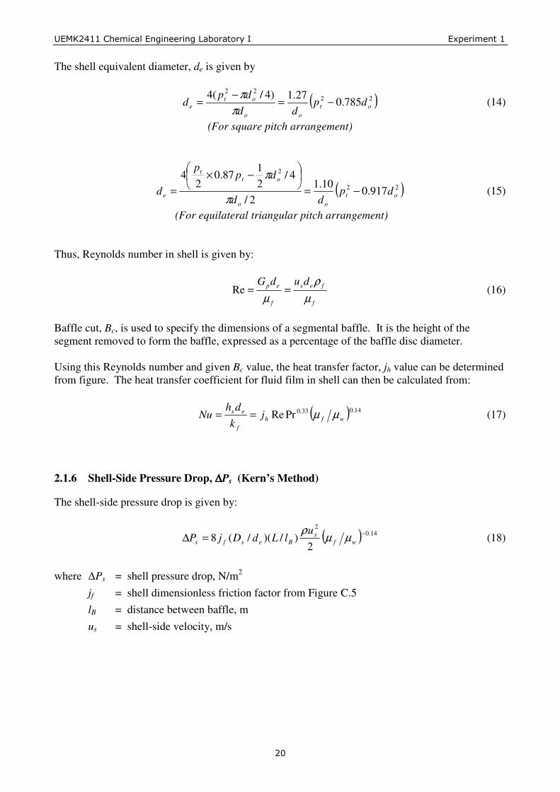
The shell equivalent diameter, de is given by
( )2222
785.027.1)4/(4
otoo
ote dp
dddp
d −=−
=π
π (14)
(For square pitch arrangement)
( )22
2
917.010.1
2/
4/21
87.02
4
otoo
ott
e dpdd
dpp
d −=��
���
� −×=
π
π (15)
(For equilateral triangular pitch arrangement) Thus, Reynolds number in shell is given by:
f
fes
f
ep dudG
µρ
µ==Re (16)
Baffle cut, Bc, is used to specify the dimensions of a segmental baffle. It is the height of the segment removed to form the baffle, expressed as a percentage of the baffle disc diameter. Using this Reynolds number and given Bc value, the heat transfer factor, jh value can be determined from figure. The heat transfer coefficient for fluid film in shell can then be calculated from:
( ) 14.033.0PrRe wfhf
es jkdh
Nu µµ== (17)
2.1.6 Shell-Side Pressure Drop, ∆∆∆∆Ps (Kern’s Method)
The shell-side pressure drop is given by:
( ) 14.02
2)/)(/(8 −=∆ wf
sBesfs
ulLdDjP µµρ
(18)
where �Ps = shell pressure drop, N/m2 jf = shell dimensionless friction factor from Figure C.5 lB = distance between baffle, m us = shell-side velocity, m/s

����������� ������� ���� ���������������� � �!"�� �������
���
2.2 Plate Heat Exchanger
Plate heat exchangers are used extensively in the food and beverage industries due to the fact that they are easily taken apart for cleaning and inspection. Their used in other industries will depend on the relative cost as compared to other types of heat exchanger such as the shell and tube heat exchangers. The general equation for heat transfer across a surface is: mTUAQ ∆= (12) where Q = heat transfer per unit time, W U = the overall heat transfer coefficient, W/m2 °C A = heat transfer area, m2
∆Tm = the mean temperature difference, the temperature driving force, °C For counter-current arrangement, the temperature difference correction factor Ft will be close to 1. Therefore, lmm TT ∆=∆ (13)
where ∆Tlm = log mean temperature difference = ( ) ( )
( )( )12
21
1221
lntTtT
tTtT
−−
−−− (14)
T1 = inlet hot water temperature T2 = outlet hot water temperature t1 = inlet cold water temperature t2 = outlet cold water temperature From heat balance, TmCQ p ∆= (15) where m = mass flow rate of fluid in the plates, kgs-1 Cp = specific heat of fluid in the plates, kJ kg-1 °C-1
∆T = temperature difference of fluid entering/leaving the plates, °C
����������� ������� ���� ���������������� � �!"�� �������
���
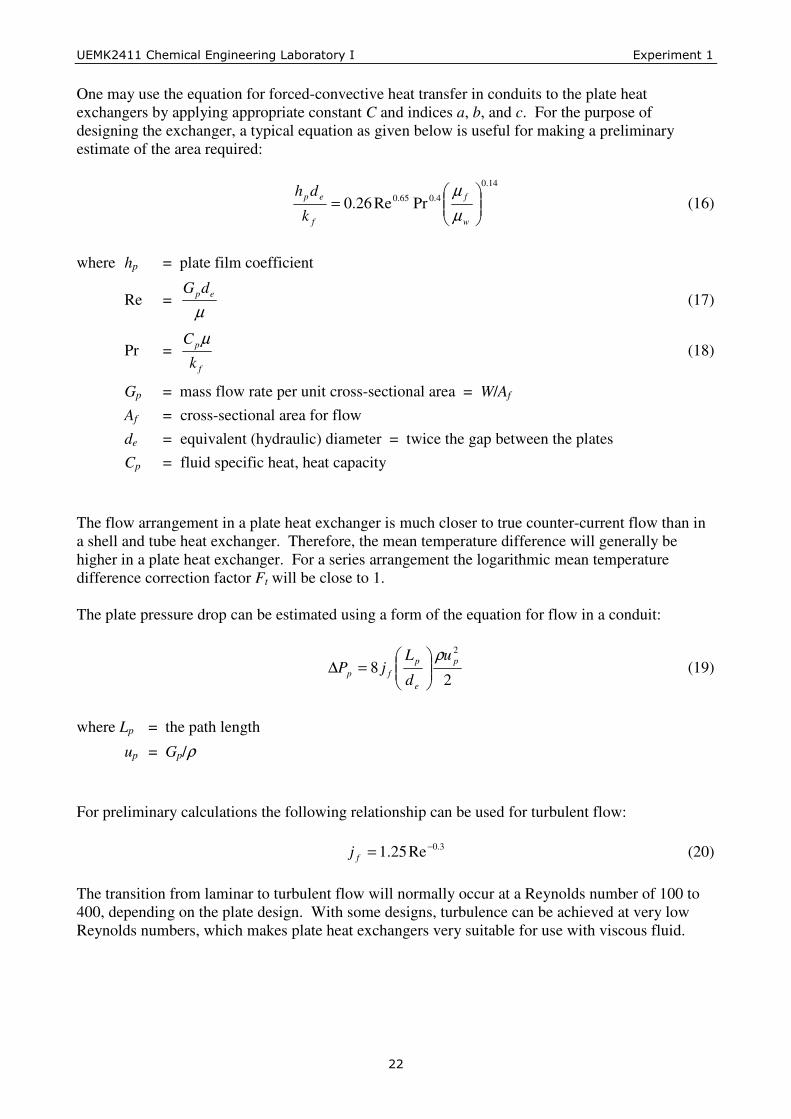
One may use the equation for forced-convective heat transfer in conduits to the plate heat exchangers by applying appropriate constant C and indices a, b, and c. For the purpose of designing the exchanger, a typical equation as given below is useful for making a preliminary estimate of the area required:
14.0
4.065.0 PrRe26.0 ���
����
�=
w
f
f
ep
k
dh
µµ
(16)
where hp = plate film coefficient
Re = µ
epdG (17)
Pr = f
p
k
C µ (18)
Gp = mass flow rate per unit cross-sectional area = W/Af
Af = cross-sectional area for flow de = equivalent (hydraulic) diameter = twice the gap between the plates Cp = fluid specific heat, heat capacity The flow arrangement in a plate heat exchanger is much closer to true counter-current flow than in a shell and tube heat exchanger. Therefore, the mean temperature difference will generally be higher in a plate heat exchanger. For a series arrangement the logarithmic mean temperature difference correction factor Ft will be close to 1. The plate pressure drop can be estimated using a form of the equation for flow in a conduit:
2
82p
e
pfp
u
d
LjP
�
����
�=∆ (19)
where Lp = the path length
up = Gp/ρ For preliminary calculations the following relationship can be used for turbulent flow: 3.0Re25.1 −=fj (20) The transition from laminar to turbulent flow will normally occur at a Reynolds number of 100 to 400, depending on the plate design. With some designs, turbulence can be achieved at very low Reynolds numbers, which makes plate heat exchangers very suitable for use with viscous fluid.
����������� ������� ���� ���������������� � �!"�� �������
���
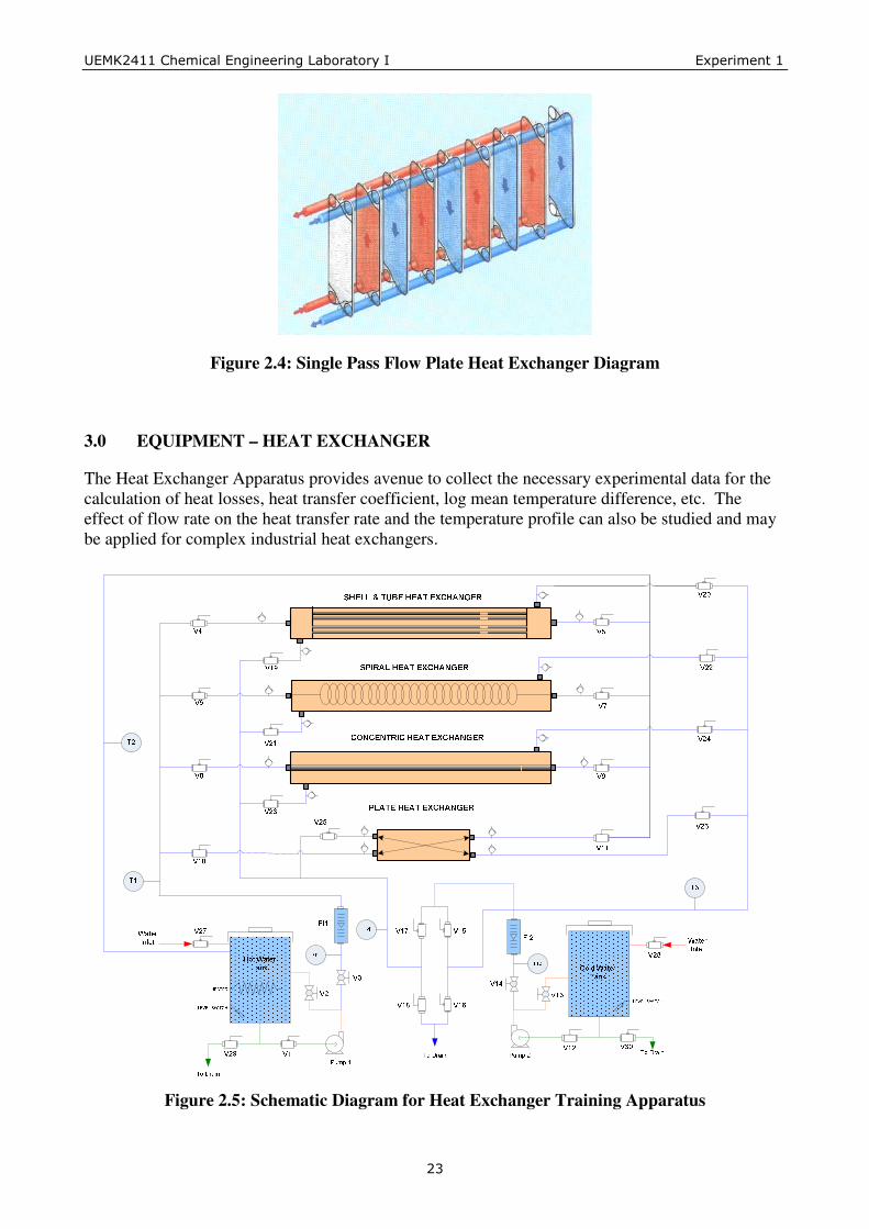
Figure 2.4: Single Pass Flow Plate Heat Exchanger Diagram
3.0 EQUIPMENT – HEAT EXCHANGER
The Heat Exchanger Apparatus provides avenue to collect the necessary experimental data for the calculation of heat losses, heat transfer coefficient, log mean temperature difference, etc. The effect of flow rate on the heat transfer rate and the temperature profile can also be studied and may be applied for complex industrial heat exchangers.
Figure 2.5: Schematic Diagram for Heat Exchanger Training Apparatus

����������� ������� ���� ���������������� � �!"�� �������
���
This unit consists of four different types of heat exchangers and two sump tanks for hot and cold water source. The hot tank is fitted with an immersion type heater that is protected against possible over heating. Each tank has a centrifugal pump which is protected from dry-run by electronic level switches. The four heat exchangers supplied with the unit are:
a) Shell and Tube Heat Exchanger
b) Spiral Heat Exchanger
c) Concentric (Double Pipe) Heat Exchanger
d) Plate Heat Exchanger
All necessary electronic sensors are fitted at respective locations for measuring the inlet and outlet temperatures of the hot and cold water, and also the flow rates of the hot and cold water streams. Digital indicators are provided on the control panel to read the appropriate data.
3.1 Process Instruments Configuration
3.1.1 Temperature Controller
The first line displays the liquid temperature in the tank while the second line displays the set value. Adjust the set value as follows:
� Press the ENT button, and then press UP or DOWN arrow key continuously until almost near the desired set value.
� Press UP or DOWN arrow key one by one until desired set value is reached. Notice that the least digit point is flashing.
� Press ENT to register the data. Notice that the least digit point goes off.
3.1.2 Valve Arrangements
Table 2.1: Valves Arrangement for Flow Selection
OPEN CLOSE
Co-Current V1, V12, V15, V18, V28 V16, V17, V27, V29, V30
Counter-Current V1, V12, V16, V17, V28 V15, V18, V27, V29, V30

����������� ������� ���� ���������������� � �!"�� �������
���
Table 2.2: Valves Arrangement for Heat Exchanger Selection
OPEN CLOSE
Shell & Tube Heat Exchanger V4, V5, V19, V20 V6 - V11, V21 - V26
Spiral Heat Exchanger V6, V7, V21, V22 V4, V5, V8 - V11, V19, V20, V23 - V26
Concentric Heat Exchanger V8, V9, V23, V24 V4 - V7, V10, V11, V19 to V22, V25, V26
Plate Heat Exchanger V10, V11, V25, V26 V4 - V9, V19 to V24
Valve V3 : to vary hot water flow rate
Valve V14 : to vary cold water flow rate
Valve V2 & V13 : flow bypass for water pump. These valves should be partially opened all the time. If the water flow rates are not stable, reduce the bypass.
3.1.3 Flow Measurements
FT1: Hot water flow rate
FT2: Cold water flow rate
The flow rates are digitally displayed in LPM.
3.1.4 Temperature Measurements
Counter-Current
TT1: Hot water inlet temperature
TT2: Hot water outlet temperature
TT3: Cold water inlet temperature
TT4: Cold water outlet temperature
Co-Current
TT1: Hot water inlet temperature
TT2: Hot water outlet temperature
TT3: Cold water outlet temperature
TT4: Cold water inlet temperature
3.1.5 Operating Limits
Temperature: maximum 70ºC

����������� ������� ���� ���������������� � �!"�� �������
���
4.0 OPERATING PROCEDURES
4.1 Pre-experiment Procedures
1. Read and understand the theory of heat exchanger.
2. Read and understand the equipment used in the experiment (heat exchanger apparatus).
3. Read the safety precautions before conducting the experiment.
4.2 General Start-Up Procedures
1. Perform a quick inspection to make sure that the equipment is in a proper working condition.
2. Be sure that all valves are initially closed, except V1 and V12.
3. Fill up hot water tank via a water supply hose connected to valve V27. Once the tank is full, close the valve.
4. Fill up the cold-water tank by opening valve V28 and leave the valve opened for continuous water supply.
5. Connect a drain hose to the cold water drain point.
6. Switch on the main power.
7. Switch on the hot water tank heater and set the temperature to 50°C. (Note: Recommended maximum temperature set point is 70°°°°C)
8. Allow the water temperature in the hot water tank to reach the set point.
9. The equipment is now ready.
4.3 General Shutdown Procedures
1. Switch off the heater and wait until the hot water temperature drops below 40°C.
2. Switch off pump P1 and pump P2.
3. Switch off the main power.
4. Drain off all the water in the process lines. Retain water in the hot and cold water tanks for next laboratory session. (Note: If the equipment is not to be run for a long period, drain all water completely.)
5. Close all valves.
5.0 SAFETY PRECAUTIONS
� Always check and rectify any leak.
� Always make sure that the heater is fully immersed in the water.
� Do not touch the hot components of the unit.
� Be extremely careful when handling liquid at high temperature.
� Always switch off the heater and allow the liquid to cool down before draining.

����������� ������� ���� ���������������� � �!"�� �������
���
6.0 EXPERIMENTS
6.1 Experiment 1A: Counter-Current Shell & Tube Heat Exchanger
In this experiment, cold water enters the shell at room temperature while hot water enters the tubes in the opposite direction. Students shall vary the hot water and cold water flow rates and record the inlet and outlet temperatures of both the hot water and cold water streams at steady state.
1. Perform the general start-up procedures as per Section 4.2.
2. Switch the valves to counter-current Shell & Tube Heat Exchanger arrangement (refer to Section 3.1).
3. Switch on pumps P1 and P2.
4. Open and adjust valves V3 and V14 to obtain the desired flow rates for hot water and cold water streams, respectively.
5. Allow the system to reach steady state for 10 minutes.
6. Record FT1, FT2, TT1, TT2, TT3 and TT4.
7. Record the pressure drop for both the shell-side and tube-side.
8. Repeat Step 4 to Step 7 for different combinations of flow rate FT1 and FT2 as shown in the table below.
6.1.1 Experimental Datasheet
FT1 (LPM)
FT2 (LPM)
TT1 (°C)
TT2 (°C)
TT3 (°C)
TT4 (°C)
DP (mmHg)
DP (mmH2O)
10 2 10 4 10 6 10 8 10 10
FT1 (LPM)
FT2 (LPM)
TT1 (°C)
TT2 (°C)
TT3 (°C)
TT4 (°C)
DP (mmHg)
DP (mmH2O)
2 10 4 10 6 10 8 10
10 10
����������� ������� ���� ���������������� � �!"�� �������
���
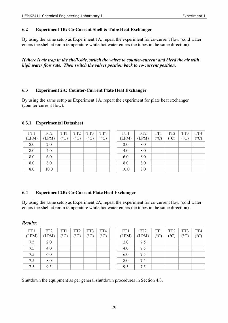
6.2 Experiment 1B: Co-Current Shell & Tube Heat Exchanger
By using the same setup as Experiment 1A, repeat the experiment for co-current flow (cold water enters the shell at room temperature while hot water enters the tubes in the same direction).
If there is air trap in the shell-side, switch the valves to counter-current and bleed the air with high water flow rate. Then switch the valves position back to co-current position.
6.3 Experiment 2A: Counter-Current Plate Heat Exchanger
By using the same setup as Experiment 1A, repeat the experiment for plate heat exchanger (counter-current flow).
6.3.1 Experimental Datasheet
FT1 (LPM)
FT2 (LPM)
TT1 (°C)
TT2 (°C)
TT3 (°C)
TT4 (°C)
FT1 (LPM)
FT2 (LPM)
TT1 (°C)
TT2 (°C)
TT3 (°C)
TT4 (°C)
8.0 2.0 2.0 8.0 8.0 4.0 4.0 8.0 8.0 6.0 6.0 8.0 8.0 8.0 8.0 8.0 8.0 10.0 10.0 8.0
6.4 Experiment 2B: Co-Current Plate Heat Exchanger
By using the same setup as Experiment 2A, repeat the experiment for co-current flow (cold water enters the shell at room temperature while hot water enters the tubes in the same direction).
Results:
FT1 (LPM)
FT2 (LPM)
TT1 (°C)
TT2 (°C)
TT3 (°C)
TT4 (°C)
FT1 (LPM)
FT2 (LPM)
TT1 (°C)
TT2 (°C)
TT3 (°C)
TT4 (°C)
7.5 2.0 2.0 7.5 7.5 4.0 4.0 7.5 7.5 6.0 6.0 7.5 7.5 8.0 8.0 7.5 7.5 9.5 9.5 7.5
Shutdown the equipment as per general shutdown procedures in Section 4.3.

����������� ������� ���� ���������������� � �!"�� �������
���
7.0 RESULTS ANALYSIS AND DISCUSSIONS
Discuss all your results. The questions below only serve as a guideline. Your discussion should not only limited to these questions.
1. Calculate the heat transfer and heat loss for energy balance study.
2. Calculate the LMTD.
3. Calculate heat transfer coefficients.
4. Calculate the pressure drop and compare with the experimental result.
5. Perform temperature profile study and the flow rate effects on heat transfer.

����������� ������� ���� ���������������� � �!"�� �������
� �
Experiment 2
Vapour-Liquid Equilibrium (VLE)
1.0 OBJECTIVES OF EXPERIMENT
� To find VLE relationship for binary mixture.
� To plot the equilibrium curve.
2.0 INTRODUCTION
Vapour-liquid equilibrium (VLE) is defined by the condition where a liquid and its vapour phase are in equilibrium with each other. Under this state or condition, there is no net change in vapour-liquid phases thus the rate of evaporation (liquid to vapour) is equal to the rate of condensation (vapour to liquid). In theory, the state of equilibrium would take forever to be reached but such equilibrium can be practically achieved within a closed system where the liquid and vapour are allowed to stand in contact with each other long enough with literally no interference or only slight interference from the exteriors.
2.1 Theory
The concentration of a vapour in contact with its liquid, especially at equilibrium, is often given by the vapour pressure. The equilibrium vapour pressure of a liquid is very much dependent on temperature. In the state of equilibrium, a liquid mixture with individual components in certain composition will have an equilibrium vapour in which the partial pressures of the vapour components will have certain set values depending on all of the liquid component compositions and the temperature. This is also true in reverse whereby a vapour with components at certain composition or partial pressure is in equilibrium with its liquid, thus the component composition of its liquid will be dependent on the vapour composition and the temperature. The equilibrium composition of each component in the vapour phase is often different from the composition of its liquid phase without a correlation. Such equilibrium phase data can be determined from a simple experiment with multicomponents of vapour-liquid mixtures. Most binary component mixtures' equilibrium data can be found in texts and references. In certain cases, estimation or prediction of equilibrium data behaviour can be done using theories such as Dalton's Law, Raoult’ s Law or Henry's Law. In multicomponent mixtures, the compositions of each component are compared in both the liquid and vapour phases where the compositions are expressed in mole fractions. A mole fraction is the number of moles of a certain component divided by the total number of moles of all components in the mixture in either the liquid or vapour phase. VLE data are often produced and shown in two component systems (binary) and three component systems (ternary). However, VLE data can exist in higher order of components but would be complex and difficult to illustrate graphically.

����������� ������� ���� ���������������� � �!"�� �������
���
2.2 Related Process Parameters
2.2.1 Vapour Pressure
Vapour pressure is defined as the pressure exerted by the gaseous phase under equilibrium state. It depends significantly on the surrounding temperature. In addition, it is known as partial pressure of a component when there is a mixture of gases present within the vapour. A vapour with components at certain concentration will have a corresponding equilibrium liquid concentration. The concentration or partial pressure of the liquid components will have certain set of values depending on the vapour component concentrations and the operating temperature. Similarly, this also applies to liquid with components. For ideal gas the partial pressure of Component 1 (p1) is given by Dalton's law, 111 Pyp = (1) Raoult's Law expressed the partial pressure in terms of vapour pressure of the liquid where vapPxp 111 = (2) However, this law is only applicable to ideal solutions with high value of x1. Generally a point is reached where the vapour pressure no longer follows the ideal relationship as x1 gradually decreases. Both Dalton and Raoult's Laws can be combined to yield an equation that relates the vapour and liquid compositions:
PPx
yvap
111 = (3)
For a dilute real solution, Henry's Law is used to determine the partial pressure of the component: 11 xKp = (4) where K is the Henry's constant but it is not equal to the vapour pressure of pure solute.

����������� ������� ���� ���������������� � �!"�� �������
���
2.2.2 Non-ideal Behaviour
For non-ideal system whereby the mixtures no longer obey Raoult's law or Henry's law, activity coefficient, γ is used to relate x1, y1, vapP1 and P as follows:
PPx
yvap
1111
γ= (5)
The liquid phase activity coefficients depend on temperature, pressure and concentration.
2.2.3 Temperature
Temperature has an effect on the VLE of a system since at different temperatures there will be a corresponding set of liquid and vapour compositions under a constant pressure. These two compositions are in equilibrium with one another at that particular point. For an ideal binary mixture, the relationship between T-x-y at a constant pressure can be represented in a plot called the phase diagram as depicted in Figure 2.1 below:
Figure 2.1: Phase Diagram At a particular temperature T1, there will be a corresponding equilibrium composition x1 and y1 for the liquid and vapour phase respectively.
x1 y1
vapour
liquid
Temperature
T

����������� ������� ���� ���������������� � �!"�� �������
���
2.2.4 Relative Volatility
Relative volatility, α12 is an indication on how easily or difficult a particular separation will be. It is a measure of the difference volatilities between two components (1 and 2). Ideally, relative volatility can be defined as the ratio of fraction of a component in the vapour phase to that in the liquid phase where it could be represented as follows:
22
1112 /
/xyxy
=α (6)
For a binary mixture, the relation can be simplified to:
( ) 112
1121 11 x
xy
−+=
αα
(7)
This relation is only valid when α12 is constant. In actual cases, it varies with temperature (increases as temperature falls). Yet it remains remarkably steady for many systems.
2.3 Theory on Refractive Index
When a chopstick is dipped in water in a glass, it looks bent. If the chopstick is dipped in thick sugar water, it looks more bent. This phenomenon arises from the refraction of light beam. An-increase in concentration of a solution will yield a higher refractive index. When the refractive index of air at the atmospheric pressure is “ 1” and a beam of light penetrates a certain medium %, the ratio between the sine of refraction angle β and the sine of incident angle α a to the normal line is called the refractive index of the medium.
Figure 2.1: Refraction of Light Beam Since refractive index varies depending on wavelength of light and temperature, it is expressed as
tDn , where n = refractive index, t = temperature, D = D-ray of sodium (589 nm).
air
medium X
1=n
βα
sinsin=Xn
α
β

����������� ������� ���� ���������������� � �!"�� �������
���
When the refractive index of water whose temperature is 20°C is measured with D-ray, it is expressed as: nD
20 = 1.33299 or usually expressed as nD = 1.33299. The result for the refractometer calibration for 2-propanol-water is given in the table below:
Table 2.1: Refractometer Calibration for 2-propanol-Water System
Water (ml) 2-Propanol (ml) Mole fraction Average RI 10 0.05 1.334700 20 0.10 1.337167 30 0.15 1.340333 40 0.20 1.343833 50 0.25 1.344800 60 0.30 1.346667 70 0.35 1.348867 80 0.40 1.350633
100 0.50 1.353667 120 0.60 1.356133 140 0.70 1.358467 160 0.80 1.360033 180 0.90 1.361800 200 1.00 1.362800 240 1.20 1.365300 280 1.40 1.367000 320 1.60 1.367900 360 1.80 1.369800 400 2.00 1.370967 440 2.20 1.371367 480 2.40 1.372000 500 2.50 1.372467 550 2.75 1.373233 600 3.00 1.373667
200
700 3.50 1.374800

����������� ������� ���� ���������������� � �!"�� �������
���
3.0 EQUIPMENT – VAPOUR-LIQUID EQUILIBRIUM APPARATUS
The vapour-liquid equilibrium apparatus is designed to study the vapour and liquid equilibrium of mixtures. The composition relationship between vapour and liquid equilibrium for binary and multicomponent mixtures at atmospheric and elevated pressures can be determined. The unit comprised of a main insulated evaporator made of stainless steel connected to an overhead condenser. The cooling water flow rate into the condenser can be regulated with a gate valve and is measured with a flow meter. A coil heater provides the necessary heat to evaporate the liquid mixture with preset temperatures controlled by a digital temperature controller. Vapour rises to the top of the unit is then condensed in the condenser. Vapour and liquid products are collected in a stainless steel vessel located at the sampling port lines. A feed port for dosing and sampling ports are provided. Digital meters are installed on the control panel to display the temperatures and pressures in the system. A pressure relief valve is connected to the unit to ensure the system will not be over-pressured at all time. Full jacket insulation ensures minimal heat loss within the unit.
Figure 3.1: Vapour-Liquid Equilibrium Apparatus
4.0 OPERATING PROCEDURES
4.1 Pre-experiment Procedures
1. Read and understand the theory of vapour-liquid equilibrium.
2. Read and understand the equipment used in the experiment (VLE apparatus).
3. Read the safety precautions and chemical hazards before conducting the experiment.
Liquid Samplingand Drain
Cooling Water Inlet Valve
Vapour Sampling
Evaporator Inlet
Insulated Stainless Steel Evaporator
Condenser
Pressure Relief Valve Temperature Meter
and Controller
Pressure Meter
Control Panel
Cooling Water Drain

����������� ������� ���� ���������������� � �!"�� �������
���
4. Read the Material Safety Data Sheet (MSDS) for the chemicals used in the experiment in Appendix A – 2-propanol.
5. Prepare the following apparatus and materials needed for the experiment:
� Refractometer
� Beakers
� Syringe / Dripper
� Prepare 7 L of 25 v/v% 2-propanol-water mixture
5.0 CHEMICAL HAZARDS, SAFETY AND PRECAUTIONS
5.1 Chemical Hazards (refer MSDS in Appendix A for more details)
� Propanol is very flammable. It evaporates readily, so it is possible for dangerous levels of vapour to build up, perhaps reaching a point at which an explosion is possible if a source of ignition is present.
� If propanol is in contact with oxygen over a long period, explosive peroxides may be formed. These typically have a higher boiling point than propanol, so may become concentrated in the liquid if propanol is distilled. Therefore, bottles of propanol, once opened, should not be stored indefinitely, in order to avoid any risk of peroxide formation.
� 2-propanol is very flammable. It can be ignited by flames, but also by contact with items such as hot plates or hot air guns.
5.2 Safety Precautions
� Always wear safety glasses, mask and gloves when handling chemicals. Do not allow the solution to come into contact with your skin or eyes.
� Should any chemicals come into contact with the body, rinse off immediately with plenty of water and inform the laboratory instructor/officer. Seek medical treatment if symptoms persist.
� Ensure that there is no source of ignition, such as a Bunsen burner, gas flame, hot plate, hot air gun or hot water pipe near the working area.
� Propanol releases irritating vapours; avoid inhalation and work in a well-ventilated area.
� Good ventilation is essential so that it is not possible for high concentrations of alcohol vapour to form.
� Dispose of all unused chemicals in an appropriate manner after the experiment. Under no circumstances should the chemicals be allowed to flow into sinks or drains.
� Wash your hands thoroughly with soap after the experiment.
� Do not switch on the heater if there is no liquid in the evaporator.
� Do not pressurise the apparatus for more than 10 bars.
� Do not boil the liquid in the apparatus for more than 200°C.
� Do not touch the evaporator (it is hot) and condenser when conducting the experiment.

����������� ������� ���� ���������������� � �!"�� �������
���
� Be careful when pouring the test liquid into the evaporator vessel.
� Be careful when taking the sample from the sampling port as the product is hot.
6.0 EXPERIMENTS
6.1 Experiment 1A: Vapour-Liquid Equilibrium
1. Close the liquid sampling and drain valve.
2. Open the vapour sampling valve and the evaporator inlet valve.
3. Pour 2-propanol-water mixture into the evaporator. (Caution: The person who pours the mixture should wear a face shield.)
4. Close the vapour sampling valve and the evaporator inlet valve.
5. Turn on the power supply and main power switch at the front of the control panel.
6. Set the temperature to 75°C.
7. Connect the cooling water drain port to drain.
8. Connect the laboratory water supply to the cooling water supply port. Tighten it with clip.
9. Switch on the heater power supply located at the control panel.
10. Turn on the water supply and allow the water to flow into the condenser. Set the water flow rate to 12 LPM.
11. Keep an eye on the temperature. When the temperature reaches the set point, wait for another 5 minutes to allow the system to reach equilibrium, and then record down the temperature and pressure.
12. Take a sample solution from the vapour sampling port and the liquid sampling port. (Caution: Be careful when taking the sample from the valves.)
13. Label the samples (i.e. temperature, pressure, x-component, y-component).
14. Close both vapour and liquid sampling valves.
15. Use a refractometer to determine the samples' refractive index (RI). (Reminder: You must take a few readings to obtain the average reading.)
16. Repeat Step 11 to Step 15 with 5°C increment until the set temperature reaches 95°C.
����������� ������� ���� ���������������� � �!"�� �������
���
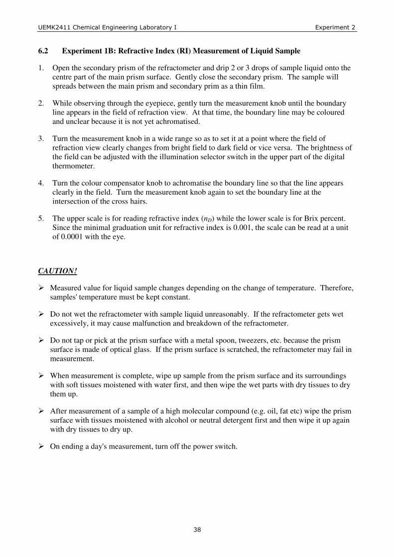
6.2 Experiment 1B: Refractive Index (RI) Measurement of Liquid Sample
1. Open the secondary prism of the refractometer and drip 2 or 3 drops of sample liquid onto the centre part of the main prism surface. Gently close the secondary prism. The sample will spreads between the main prism and secondary prim as a thin film.
2. While observing through the eyepiece, gently turn the measurement knob until the boundary line appears in the field of refraction view. At that time, the boundary line may be coloured and unclear because it is not yet achromatised.
3. Turn the measurement knob in a wide range so as to set it at a point where the field of refraction view clearly changes from bright field to dark field or vice versa. The brightness of the field can be adjusted with the illumination selector switch in the upper part of the digital thermometer.
4. Turn the colour compensator knob to achromatise the boundary line so that the line appears clearly in the field. Turn the measurement knob again to set the boundary line at the intersection of the cross hairs.
5. The upper scale is for reading refractive index (nD) while the lower scale is for Brix percent. Since the minimal graduation unit for refractive index is 0.001, the scale can be read at a unit of 0.0001 with the eye.
CAUTION!
� Measured value for liquid sample changes depending on the change of temperature. Therefore, samples' temperature must be kept constant.
� Do not wet the refractometer with sample liquid unreasonably. If the refractometer gets wet excessively, it may cause malfunction and breakdown of the refractometer.
� Do not tap or pick at the prism surface with a metal spoon, tweezers, etc. because the prism surface is made of optical glass. If the prism surface is scratched, the refractometer may fail in measurement.
� When measurement is complete, wipe up sample from the prism surface and its surroundings with soft tissues moistened with water first, and then wipe the wet parts with dry tissues to dry them up.
� After measurement of a sample of a high molecular compound (e.g. oil, fat etc) wipe the prism surface with tissues moistened with alcohol or neutral detergent first and then wipe it up again with dry tissues to dry up.
� On ending a day's measurement, turn off the power switch.

����������� ������� ���� ���������������� � �!"�� �������
���
Results:
Mixture Condenser water flow rate Temperature
(°°°°C) Pressure
(bar) Reading 1 Reading 2 Reading 3 Average
Vapour RI Liquid RI Vapour RI Liquid RI Vapour RI Liquid RI Vapour RI Liquid RI Vapour RI Liquid RI Vapour RI Liquid RI
Temperature (°°°°C)
Pressure (bar) Average
Reading Corresponding Mole Fraction Reading
Vapour RI Vapour (y) Liquid RI Liquid (x) Vapour RI Vapour (y) Liquid RI Liquid (x) Vapour RI Vapour (y) Liquid RI Liquid (x) Vapour RI Vapour (y) Liquid RI Liquid (x) Vapour RI Vapour (y) Liquid RI Liquid (x) Vapour RI Vapour (y) Liquid RI Liquid (x)
Temperature (°°°°C) Pressure (bar) Vapour Mole Fraction (y) Liquid Mole Fraction (x)
����������� ������� ���� ���������������� � �!"�� �������
� �
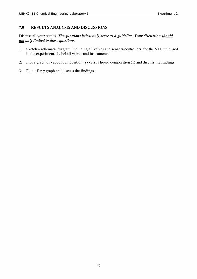
7.0 RESULTS ANALYSIS AND DISCUSSIONS
Discuss all your results. The questions below only serve as a guideline. Your discussion should not only limited to these questions.
1. Sketch a schematic diagram, including all valves and sensors/controllers, for the VLE unit used in the experiment. Label all valves and instruments.
2. Plot a graph of vapour composition (y) versus liquid composition (x) and discuss the findings.
3. Plot a T-x-y graph and discuss the findings.
����������� ������� ���� ���������������� � �!"�� �������
���
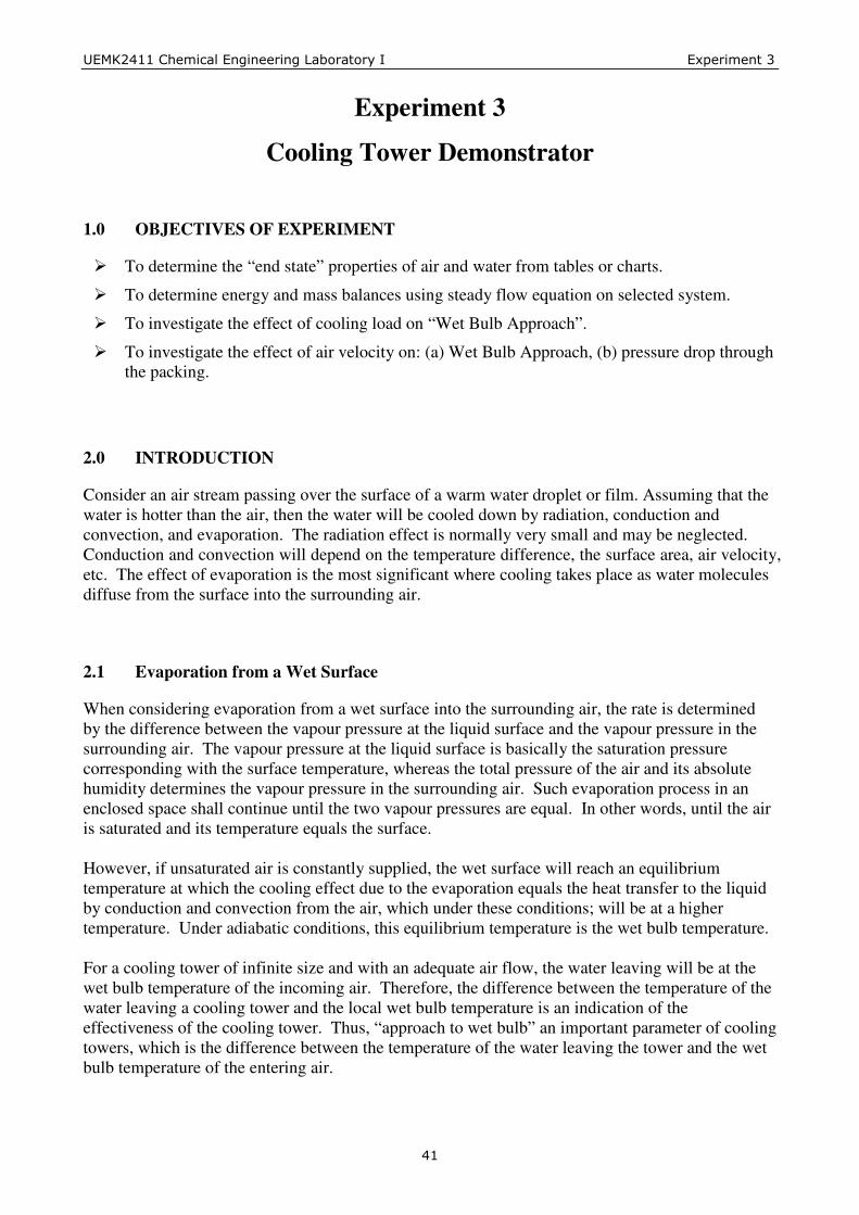
Experiment 3
Cooling Tower Demonstrator
1.0 OBJECTIVES OF EXPERIMENT
� To determine the “ end state” properties of air and water from tables or charts.
� To determine energy and mass balances using steady flow equation on selected system.
� To investigate the effect of cooling load on “ Wet Bulb Approach” .
� To investigate the effect of air velocity on: (a) Wet Bulb Approach, (b) pressure drop through the packing.
2.0 INTRODUCTION
Consider an air stream passing over the surface of a warm water droplet or film. Assuming that the water is hotter than the air, then the water will be cooled down by radiation, conduction and convection, and evaporation. The radiation effect is normally very small and may be neglected. Conduction and convection will depend on the temperature difference, the surface area, air velocity, etc. The effect of evaporation is the most significant where cooling takes place as water molecules diffuse from the surface into the surrounding air.
2.1 Evaporation from a Wet Surface
When considering evaporation from a wet surface into the surrounding air, the rate is determined by the difference between the vapour pressure at the liquid surface and the vapour pressure in the surrounding air. The vapour pressure at the liquid surface is basically the saturation pressure corresponding with the surface temperature, whereas the total pressure of the air and its absolute humidity determines the vapour pressure in the surrounding air. Such evaporation process in an enclosed space shall continue until the two vapour pressures are equal. In other words, until the air is saturated and its temperature equals the surface. However, if unsaturated air is constantly supplied, the wet surface will reach an equilibrium temperature at which the cooling effect due to the evaporation equals the heat transfer to the liquid by conduction and convection from the air, which under these conditions; will be at a higher temperature. Under adiabatic conditions, this equilibrium temperature is the wet bulb temperature. For a cooling tower of infinite size and with an adequate air flow, the water leaving will be at the wet bulb temperature of the incoming air. Therefore, the difference between the temperature of the water leaving a cooling tower and the local wet bulb temperature is an indication of the effectiveness of the cooling tower. Thus, “ approach to wet bulb” an important parameter of cooling towers, which is the difference between the temperature of the water leaving the tower and the wet bulb temperature of the entering air.
����������� ������� ���� ���������������� � �!"�� �������
���
2.2 Cooling Tower Performance
A study on the performance of a cooling tower is to verify the effect of the following factors on the cooling tower performance:
� water flow rates
� water temperatures
� air flow rate
� inlet air relative humidity
The effect of these factors will be studied in depth by varying them. In this way, we can gain an overall view of the operation of the cooling tower.
2.3 Thermodynamic Property
In order to understand the working principle and performance of a cooling tower, a basic knowledge of thermodynamic is essential. A brief review on some of the thermodynamic properties is presented below.
2.3.1 Specific Enthalpy
At water triple point (i.e. 0.00602 atm and 0.01°C), the specific enthalpy of saturated water is assumed to be zero, which is taken as datum. The specific enthalpy of saturated water (hi) at a range of temperatures above the datum condition can be obtained from thermodynamic tables. The specific enthalpy of compressed liquid is given by ( )satff ppvhh −+= (1) The correction for pressure is negligible for the operating conditions of a cooling tower, thus h ≈ hf at a given temperature.
2.3.2 Specific Heat Capacity, Cp
Specific heat capacity, Cp is defined as the rate of change of enthalpy with respect to temperature (often called the specific heat at constant pressure). For the purpose of experiment, we may use the following relationship: TCh p∆=∆ (2) and TCh p= (3) where Cp for water is taken as 4.18 kJ/kg⋅°C.
����������� ������� ���� ���������������� � �!"�� �������
���
2.3.3 Dalton's and Gibbs Laws
It is commonly known that air consists of a mixture of dry air (O2, N2 and other gases) and water vapour. Dalton and Gibbs Laws describe the behaviour of such a mixture as: � The total pressure of the air is equal to the sum of the pressures at which the dry air and the
water vapour each and alone would exert if they were to occupy the volume of the mixture at the temperature of the mixture.
� The dry air and the water vapour respectively obey their normal property relationships at their
partial pressures. � The enthalpy of the mixture may be found by adding together the enthalpies at which the dry air
and water vapour each would have as the sole occupant of the space occupied by the mixture and at the same temperature.
2.3.4 Humidity and Saturation
Absolute or Specific Humidity, airdry of Mass
our water vapof Mass=ω (4)
Relative Humidity, re temperatusame at theour water vapof pressure Saturation
Airin our water vapof pressure Partial=φ (5)
Percentage Saturation re temperatusame at theour water vapsat. of vol.same of Mass
Air of megiven voluin our water vapof Mass= (6)
At high humidity conditions, it can be shown that there is not much difference between the relative humidity and the percentage saturation and thus we shall regard them as the same.
2.3.5 Psychometric Chart
The psychometric chart is very useful in determining the properties of air/water vapour mixture. Among the properties that can be defined with psychometric chart are Dry Bulb Temperature, Wet Bulb Temperature, Relative Humidity, Humidity Ratio, Specific Volume and Specific Enthalpy. Knowing any two of these properties, the other properties can be easily identified from the chart provided the air pressure is approximately 1 atm.

����������� ������� ���� ���������������� � �!"�� �������
���
2.4 Orifice Calibration
Psychometric chart can be used to determine the value of the specific volume. However, the values given in the chart are for 1 kg of dry air at the stated total pressure. For every kilogram of dry air, there is w kg of water vapour, yielding the total mass of (1 + w) kg. Thus, the actual specific volume of the air/vapour mixture is given by:
ω+
=1
baa
vv (7)
The mass flow rate of air and steam mixture through the orifice is given by
( )
ba
a
vx
vx
m
ω+=
=
10137.0
0137.0&
(8)
where m& = mass flow rate of air/vapour mixture va = actual specific volume
bav = specific volume of air at the outlet
x = orifice differential, mm H2O
ω = humidity ratio of mixture The mass flow rate of dry air is given by
( )
( )ω
ωω
ω
+=
+×+
=
×+
=
10137.0
10137.0
11
mixture air/vapour of rate flow mass1
1
b
b
a
a
a
vx
vx
m&
(9)
A simplification can be made since in this application, the value of ω is unlikely to exceed 0.025. As such, neglecting wb would not yield significant error.

����������� ������� ���� ���������������� � �!"�� �������
���
2.5 Application of Steady Flow Energy Equation
Consider System A for a cooling tower as defined in Figure 2.1. It can be seen that for this system, indicated by the boundary line,
� heat transfer at the load tank and possibly a small quantity to surroundings
� work transfer at the pump
� low humidity air enters at point A
� high humidity air leaves at point B
� make-up enters at point E, the same amount as the moisture increase in the air stream
Figure 2.1: System A
From the steady flow equation,
EEAssdagssdaa
inout
hmhmhmhmhm
HHPQ
−+−+=
−=−
)( (10)
The pump power, P is a work input, therefore it is negative. If the enthalpy of the air includes the enthalpy of the steam associated with it, and this quantity is in terms of per unit mass of dry air, the equation may then be written as: EEABa hmhhmPQ && −−=− )( (11) The mass flow rate of dry air, ma through a cooling tower is constant, whereas the mass flow rate of moist air increases as the result of evaporation process. The term EEhm& can usually be neglected since its value is relatively small. Under steady state conditions, by conservation of mass, the mass flow rate of dry air and of water (as liquid or vapour) must be the same at inlet and outlet to any system. Therefore,
( ) ( )BaAa mm && = and ( ) ( )BaEAa mmm &&& =+ or ( ) ( )AaBaE mmm &&& −=

����������� ������� ���� ���������������� � �!"�� �������
���
The ratio of steam to air is known for the initial and final state points on the psychrometric charts. Therefore,
( ) AaAs mm ω&& = and ( ) BaBs mm ω&& = ( )ABaE mm ωω −= && (12) Let re-define the cooling tower system to be as in Figure 2.2 where the process heat and pump work does not cross the boundary of the system. In this case warm water enters the system at point C and cool water leaves at point D.
Figure 2.2: System B Again from the steady flow energy equation, inout HHPQ −=− , where P = 0. Q& may have a small value due to heat transfer between the unit and its surroundings: ( )EECwAaDwBa hmhmhmhmhmQ &&&& ++−+= (18) Rearranging,
( ) ( ) EECDwABa hmhhmhhmQ &&& −−−−=
( ) ( ) EECDpwABa hmttCmhhmQ &&& −−−−= (19) Again, the term EEhm& can be neglected.

����������� ������� ���� ���������������� � �!"�� �������
���
3.0 EQUIPMENT – WATER COOLING TOWER
The water cooling tower is designed to demonstrate the construction, design and operational characteristics of a modern cooling system. The unit resembles a full size forced draught cooling tower and it is actually an “ open system” through which two streams of fluid (in this case air and water) pass and in which there is a heat transfer from one stream to the other. The unit is self-contained supplied with a heating load and a circulating pump.
3.1 Load Tank
The stainless steel load tank has a capacity of 9 litres. It is fitted with two cartridge heaters, 0.5 kW and 1.0 kW each, to provide a total of 1.5 kW of cooling load. A make-up tank is fixed on top of the load tank. A float type valve at the bottom of the make-up tank is used to control the amount of water flowing into the load tank. A centrifugal type pump (work input = 40 W) is supplied for circulating water from the load tank through a flow meter to the top of the column, into a basin and back to the load tank. A temperature sensor and temperature controller is fitted at the load tank to prevent overheating. A level switch is fitted at the load tank so that the heater and pump will be switched off if a low level condition occurs.
3.2 Air Distribution Chamber
The stainless steel air distribution chamber comes with a water collecting basin and a one-side inlet centrifugal fan. The fan has a capacity of approximately 235 CFM of air flow. The air flow rate is adjusted by means of an intake damper.
3.3 Tower and Packing
The tower is made of clear acrylic with a square cross-sectional area of 225 cm2 (15 cm × 15 cm) and a height of 60 cm. The packing density of tower is 110 m2/m3 for Column A and 77 m2/m3 for Column B. It comes with eight decks of inclined packing. A top column that fitted on top of the tower comes with a sharp-edged orifice, a droplet arrester and a water distribution system.
3.4 Operation Processes
3.4.1 Water Circuit
Water temperature in load tank will be increased before the water is pumped through the control valve and flow meter to the column cap. Before entering the cap, the water inlet temperature is measured. The water is then uniformly distributed over the top packing deck. This creates a large thin film of water, which will be exposed to the air stream. The water will be cooled as it flows downward through the packing due to evaporation process. The cooled water falls into the basin below the lowest deck and return to the load tank where it is heated again before recirculation. The outlet temperature is measured at a point just before the water flows back into the load tank.

����������� ������� ���� ���������������� � �!"�� �������
���
Evaporation causes the water level in the load tank to fall. The amount of water lost by evaporation will be automatically compensated by equal amount of water from the make up tank. At steady-state, this compensation rate equals the rate of evaporation plus any small airborne droplets discharge with the air.
3.4.2 Air Circuit
A one-side inlet centrifugal fan draws the air from the atmosphere into the distribution chamber. The air flow rate can be varied by means of an intake damper. The air passes the dry and wet bulb temperature sensors before it enters the bottom of the tower. As the air stream passes through the packing, its moisture content increases and the water temperature drops. The air passed another duct detector measuring its exit temperature and relative humidity, then through a droplet arrester and an orifice before finally leaving the top of the tower into the atmosphere.
3.5 Temperature Sensors
Temperature measurements are assigned as follows:
T1 Dry Bulb Inlet Air Temperature
T2 Wet Bulb Inlet Air Temperature
T3 Dry Bulb Outlet Air Temperature
T4 Wet Bulb Outlet Air Temperature
T5 Inlet Water Temperature
T6 Outlet Water Temperature
T7 Make-up Tank Temperature
T8 Hot Water Tank Temperature
The pressure drop across the tower is measured by a differential pressure sensor. The air flow rate is measured by a differential pressure sensor and an orifice. The water flow rate is measure by a flow meter.
����������� ������� ���� ���������������� � �!"�� �������
���
4.0 OPERATING PROCEDURES
4.1 Pre-experiment Procedures
1. Read and understand the theory of cooling tower system.
2. Read and understand the equipment used in the experiment (cooling tower demonstrator).
3. Read the safety precautions before conducting the experiment.
4.2 General Operating Procedures
4.2.1 Air Flow Control
The air flow into the receiver is controlled by limiting the air suction flow at the centrifugal fan. Use to Perspex damper to control the air suction opening.
4.2.2 Heater Temperature Control
The first line displays the hot water temperature in the tank while the second line displays the set value. Adjust the set value as follows: Press UP or DOWN arrow key continuously until the desired set value is reached. The new set value will immediately take effect.
4.2.3 Measuring Differential Pressure
Check that the pressure tubing for differential pressure measurement is connected correctly. Always make sure that no water is in the pressure tubings for accurate differential pressure measurement.
To measure the differential pressure across the orifice, open valve V4, V5; close valve V3, V6.
To measure the differential pressure across the column, open valve V3, V6; close valve V4, V5.
4.3 General Start-Up Procedures
1. Ensure that valves V1 to V6 are closed and valve V7 is partially opened.
2. Fill the load tank with distilled or deionised water. It is done by first removing the make-up tank and then pours the water through the opening at the top of the load tank.
3. Replace the make-up tank onto the load tank and lightly tighten the nuts. Fill the tank with distilled or deionised water up to the zero mark on the scale.
4. Add distilled/deionised water to the wet bulb sensor reservoir to the fullest.
5. Connect all appropriate tubing to the differential pressure sensor.

����������� ������� ���� ���������������� � �!"�� �������
� �
6. Set the temperature controller set point to 50°C. Switch on the 1.0 kW water heater and heat up the water to approximately 40°C.
7. Switch on the pump and slowly open the control valve V1 and set the water flowrate to 2.0 LPM. Obtain a steady operation where the water is distributed and flowing uniformly through the packing.
8. Fully open the fan damper and then switch on the fan. Check that the differential pressure sensor is giving reading when the valve manifold is switched to measure the orifice differential pressure.
9. Let the unit run for about 20 minutes for the float valve to correctly adjust the level in the load tank. Refill the makeup tank as required.
10. The unit is now ready.
Note: It is strongly recommended that ONLY distilled or deionised water be used in this unit. The impurities existing in tap water may cause depositing in the cooling tower.
4.4 General Shutdown Procedures
1. Switch off the heaters and let the water circulate through the cooling tower system for 3 – 5 minutes until the water cooled down.
2. Switch of the fan and fully close the fan damper.
3. Switch off the pump and power supply.
4. Retain the water in reservoir tank for next experiment or completely drain off the water from the unit if it is not in used.
5.0 SAFETY PRECAUTIONS
� All operating instructions supplied must be read carefully and understood before attempting to operate the unit.
� Keep hands away from the blower when it is running to avoid serious injury.
� Do not connect the power if the unit is damaged or even partially wet.
� Do not touch the hot component of the unit.
� Do not set the heater temperature above its maximum operating temperature of 70°C to avoid pump damage.
� Do not use pliers or other tools to tighten the screws. Use only bare hands. Over tightening could damage the seals and cause leakage.
� Exercise caution when pouring water into the make up tank to ensure no water is spilt onto the electrical parts.
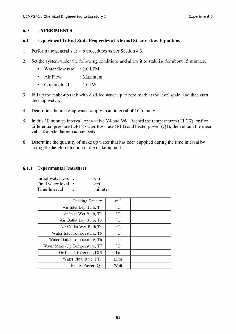
����������� ������� ���� ���������������� � �!"�� �������
���
6.0 EXPERIMENTS
6.1 Experiment 1: End State Properties of Air and Steady Flow Equations
1. Perform the general start-up procedures as per Section 4.3.
2. Set the system under the following conditions and allow it to stabilise for about 15 minutes.
� Water flow rate : 2.0 LPM
� Air Flow : Maximum
� Cooling load : 1.0 kW
3. Fill up the make-up tank with distilled water up to zero mark at the level scale, and then start the stop watch.
4. Determine the make-up water supply in an interval of 10 minutes.
5. In this 10 minutes interval, open valve V4 and V6. Record the temperatures (T1-T7), orifice differential pressure (DP1), water flow rate (FT1) and heater power (Q1), then obtain the mean value for calculation and analysis.
6. Determine the quantity of make up water that has been supplied during the time interval by noting the height reduction in the make-up tank.
6.1.1 Experimental Datasheet
Initial water level : cm Final water level : cm Time Interval : minutes
Packing Density m-1 Air Inlet Dry Bulb, T1 °C Air Inlet Wet Bulb, T2 °C
Air Outlet Dry Bulb, T3 °C Air Outlet Wet Bulb,T4 °C
Water Inlet Temperature, T5 °C Water Outlet Temperature, T6 °C
Water Make-Up Temperature, T7 °C Orifice Differential, DPI Pa
Water Flow Rate, FT1 LPM Heater Power, Q1 Watt

����������� ������� ���� ���������������� � �!"�� �������
���
6.2 Experiment 2: Investigate the Effect of Cooling Load on Wet Bulb Approach
1. Perform the general start-up procedures as per Section 4.3.
2. Set the system under the following conditions and allow it to stabilise for about 15 minutes.
� Water flow rate : 2.0 LPM
� Air Flow : Maximum
� Cooling load : 0 kW
3. After the system stabilised, open valve V4 and V6.
4. Record the air inlet dry bulb and wet bulb temperature (T1, T2), water outlet temperature (T6), orifice differential pressure (DP1), water flow rate (FT1) and heater power (Q1), then obtain the mean value for calculation and analysis (for Experiment 2B).
5. Without changing the conditions, increase the cooling load to 0.5 kW. When the system stabilised, record all the data.
6. Repeat the experiment for cooling load of 1.0 kW and 1.5 kW.
6.2.1 Experimental Datasheet
Cooling Load Description Unit 0.0 kW 0.5 kW 1.0 kW 1.5 kW
Packing Density m-1 Air Inlet Dry Bulb, T1 °C Air Inlet Wet Bulb, T2 °C
Air Outlet Dry Bulb, T3 °C Air Outlet Wet Bulb, T4 °C
Water Inlet Temperature, T5 °C Water Outlet Temperature, T6 °C
Orifice Differential, DP1 Pa Water Flow Rate, FT1 LPM
Heater Power, Q1 Watt
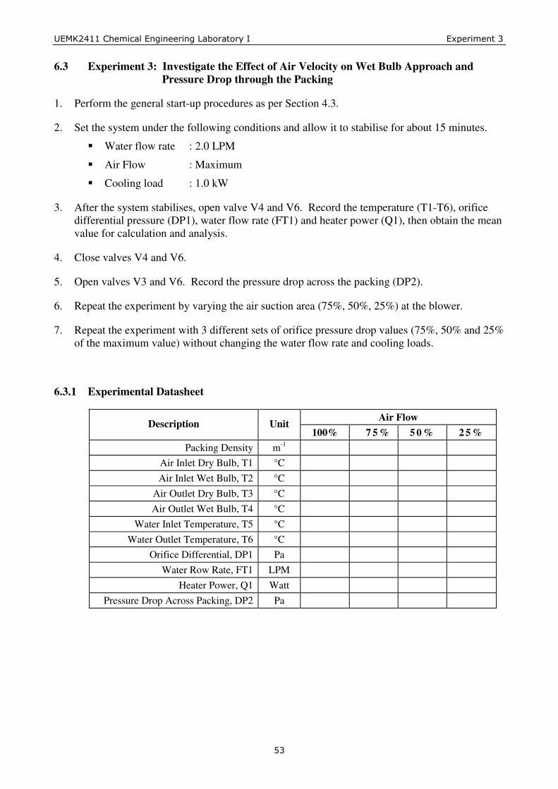
����������� ������� ���� ���������������� � �!"�� �������
���
6.3 Experiment 3: Investigate the Effect of Air Velocity on Wet Bulb Approach and Pressure Drop through the Packing
1. Perform the general start-up procedures as per Section 4.3.
2. Set the system under the following conditions and allow it to stabilise for about 15 minutes.
� Water flow rate : 2.0 LPM
� Air Flow : Maximum
� Cooling load : 1.0 kW
3. After the system stabilises, open valve V4 and V6. Record the temperature (T1-T6), orifice differential pressure (DP1), water flow rate (FT1) and heater power (Q1), then obtain the mean value for calculation and analysis.
4. Close valves V4 and V6.
5. Open valves V3 and V6. Record the pressure drop across the packing (DP2).
6. Repeat the experiment by varying the air suction area (75%, 50%, 25%) at the blower.
7. Repeat the experiment with 3 different sets of orifice pressure drop values (75%, 50% and 25% of the maximum value) without changing the water flow rate and cooling loads.
6.3.1 Experimental Datasheet
Air Flow Description Unit 100% 7 5 % 5 0 % 2 5 %
Packing Density m-1 Air Inlet Dry Bulb, T1 °C Air Inlet Wet Bulb, T2 °C
Air Outlet Dry Bulb, T3 °C Air Outlet Wet Bulb, T4 °C
Water Inlet Temperature, T5 °C Water Outlet Temperature, T6 °C
Orifice Differential, DP1 Pa Water Row Rate, FT1 LPM
Heater Power, Q1 Watt Pressure Drop Across Packing, DP2 Pa
����������� ������� ���� ���������������� � �!"�� �������
���
7.0 RESULTS ANALYSIS AND DISCUSSIONS
Discuss all your results. The questions below only serve as a guideline. Your discussion should not only limited to these questions.
1. Sketch a schematic diagram, including all valves and sensors/controllers, for the cooling water tower used in the experiment. Label all valves and instruments.
2. For Experiment 1, calculate
� the make-up rate.
� the energy and mass balances using the steady flow equation. Discuss the findings.
3. For Experiment 2,
� calculate the ‘wet bulb approach” and total cooling rate.
� plot a graph to show relationship between cooling load and “ approach to wet bulb” temperature. Discuss the findings.
4. For Experiment 3,
� calculate the nominal air velocity and find the “ approach to wet bulb” .
� plot a graph to show the relationship between ‘approach to wet bulb” and packing pressure drop versus nominal air velocity. Discuss the findings.
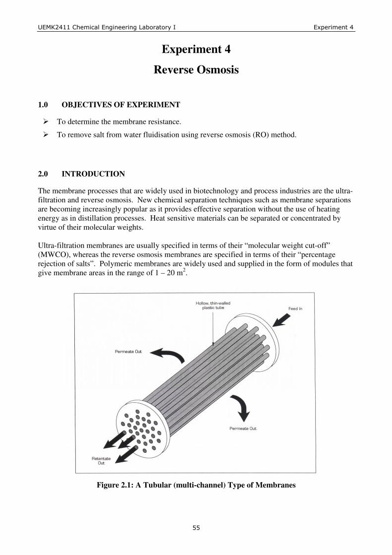
����������� ������� ���� ���������������� � �!"�� �������
���
Experiment 4
Reverse Osmosis
1.0 OBJECTIVES OF EXPERIMENT
� To determine the membrane resistance.
� To remove salt from water fluidisation using reverse osmosis (RO) method.
2.0 INTRODUCTION
The membrane processes that are widely used in biotechnology and process industries are the ultra-filtration and reverse osmosis. New chemical separation techniques such as membrane separations are becoming increasingly popular as it provides effective separation without the use of heating energy as in distillation processes. Heat sensitive materials can be separated or concentrated by virtue of their molecular weights. Ultra-filtration membranes are usually specified in terms of their “ molecular weight cut-off” (MWCO), whereas the reverse osmosis membranes are specified in terms of their “ percentage rejection of salts” . Polymeric membranes are widely used and supplied in the form of modules that give membrane areas in the range of 1 – 20 m2.
Figure 2.1: A Tubular (multi-channel) Type of Membranes
����������� ������� ���� ���������������� � �!"�� �������
���
The membranes that will be used for this experiment are classified as tubular type (Figure 2.1), which is widely used and have turbulent flow conditions. The system is in a cross flow configuration where the feed solution is pumped in-series through the membranes at a velocity in the range of 0 – 2.5 m/s with a pressure difference of 0.1 – 0.5 MPa across the membrane. Liquid permeates through the membrane and feed emerges in a more concentrated form on the exit of the module. The advantages of cross-flow membrane separations are: � Higher overall liquid removal rate is achieved by preventing solid build-up on membrane
surface
� The concentrate (retentate) remains in a mobile form suitable for further processing
� The solute content of the concentrate may be varied over a wide range
� It may also be possible to fractionate solutes of different sizes
2.1 Theory
Numerous theoretical models for ultra-filtration, nano-filtration, and reverse osmosis have been proposed along with the identification of new factors controlling flux or mass transfer through membranes. The basic operating patterns are best outlined in terms of the hydrodynamic resistance resulting from the buildup of deposited materials on the membrane surface. The flux, J will be given by
dtdV
AJ
m
1= = ( )cm RRP+
∆µ
= ( )[ ]mbm AVCRP
/αµ +∆
(1)
For most biological materials, � is a variable depending on the applied pressure and time (the compressible deposit), so that the expression requires a numerical solution. A useful method for the effects of cross-flow removal of depositing materials is to write
( )rdm RRRP
J−+
∆=µ
(2)
Removal of solute by cross-flow is sometimes assumed constant, and equal to the convective particle transport at steady state (JssCb), which can be obtained experimentally or from an appropriate model. In many situations however, steady state of filtration is seldom achieved. In such cases, it is possible to describe the time dependence of filtration by introducing an efficiency factor β, representing the fraction of filtered material remaining deposit rather than being swept along by the bulk flow. This gives
m
bc A
VCR
βα= , where 0 < β < 1 (3)

����������� ������� ���� ���������������� � �!"�� �������
���
Although deposition also occurs during ultra-filtration, an equally important factor controlling flux is concentration polarization. (Figure 2.2)
Figure 2.2: Concentration Polarization at a Membrane Surface
(Cw = solute concentration at the membrane surface, Cb, = bulk-solute concentration) Typical operating patterns are shown in Figure 2.3.
Figure 2.3: Typical Dependence of Membrane Flux
(a) Applied Pressure Difference, (b) Solute Concentration, (c) Cross-Flow Velocity Solution containing macromolecular gel-forming solute will form a gel on the surface of the membrane. The gel formation will contribute to formation of dynamic membranes. The mechanism is as follows: Due to convective flux through the membrane a concentration of the solution at the surface Cw increases and eventually reaches a gel formation concentration Cg (Figure 2.3b). The flux, J through the membrane depends on a concentration according to the relationship
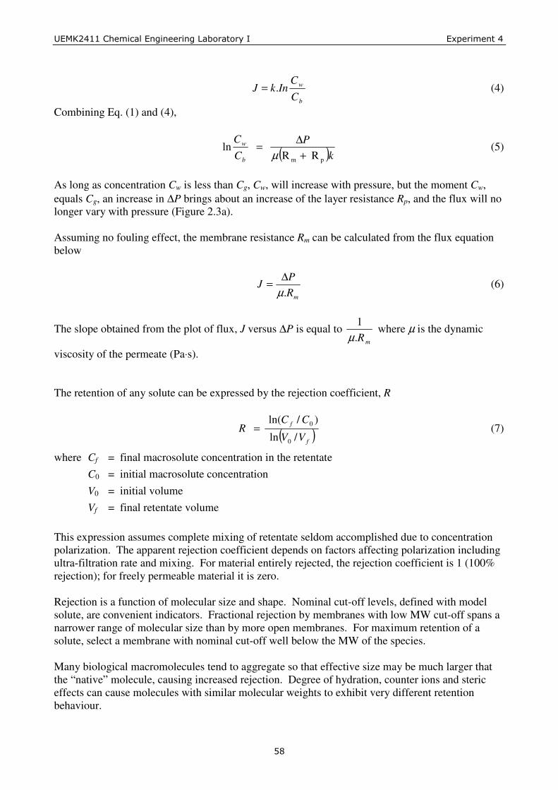
����������� ������� ���� ���������������� � �!"�� �������
���
b
w
CC
InkJ .= (4)
Combining Eq. (1) and (4),
( )kP
CC
b
w
pm R R ln
+∆=
µ (5)
As long as concentration Cw is less than Cg, Cw, will increase with pressure, but the moment Cw, equals Cg, an increase in ∆P brings about an increase of the layer resistance Rp, and the flux will no longer vary with pressure (Figure 2.3a). Assuming no fouling effect, the membrane resistance Rm can be calculated from the flux equation below
mR
PJ
.µ∆= (6)
The slope obtained from the plot of flux, J versus ∆P is equal to mR.
1µ
where µ is the dynamic
viscosity of the permeate (Pa⋅s). The retention of any solute can be expressed by the rejection coefficient, R
( )f
f
VV
CCR
/ln
)/ln(
0
0= (7)
where Cf = final macrosolute concentration in the retentate C0 = initial macrosolute concentration V0 = initial volume Vf = final retentate volume This expression assumes complete mixing of retentate seldom accomplished due to concentration polarization. The apparent rejection coefficient depends on factors affecting polarization including ultra-filtration rate and mixing. For material entirely rejected, the rejection coefficient is 1 (100% rejection); for freely permeable material it is zero. Rejection is a function of molecular size and shape. Nominal cut-off levels, defined with model solute, are convenient indicators. Fractional rejection by membranes with low MW cut-off spans a narrower range of molecular size than by more open membranes. For maximum retention of a solute, select a membrane with nominal cut-off well below the MW of the species. Many biological macromolecules tend to aggregate so that effective size may be much larger that the “ native” molecule, causing increased rejection. Degree of hydration, counter ions and steric effects can cause molecules with similar molecular weights to exhibit very different retention behaviour.

����������� ������� ���� ���������������� � �!"�� �������
���
3.0 EQUIPMENT – REVERSE OSMOSIS AND ULTRA-FILTRATION UNIT
3.1 Membrane and Membrane Housing
The P.C.I Micro 240 module is designed to be fitted to wide range of tubular ultra-filtration, nano-filtration, or reverse osmosis membranes. The module has termination points allowing easy connection by flexible or welded couplings to existing equipment. Each module comprises 2 perforated stainless steel tubes, fabricated in the form of shell and tube configuration, each tube fitted with a membrane element. The open channel, highly turbulent flow design allows a wide variety of process fluid to be concentrated. It also allows simple clean-in-place techniques to be entirely effective.
Figure 3.1: Module Assembly
Designed Operating Conditions for P.C.I Micro 240 membranes:
Permeate flow : 5 – 50 ml/min
Recommended pressure : 4 bar ( for UF), 40 bar (for RO & NF)
Recommended recycle : 30 LPM (for UF), 18 LPM (for RO & NF)
Pressure drop (water) : 2 psi @ 2 m/s, 7 psi @ 4 m/s
3.2 Pumps
The triple plunger pump (P1) is used to pump the liquid from the feed tank into the membrane module. A pressure regulator is installed to regulate the operating pressure of the feed system.
3.3 Tanks
The unit is supplied with a feed tank and a product tank, both having a maximum capacity of 30 litres. The feed and product tanks are made of stainless steel for corrosion and chemical resistance. The feed tank has a cooling system to remove the heat generated from the pump.
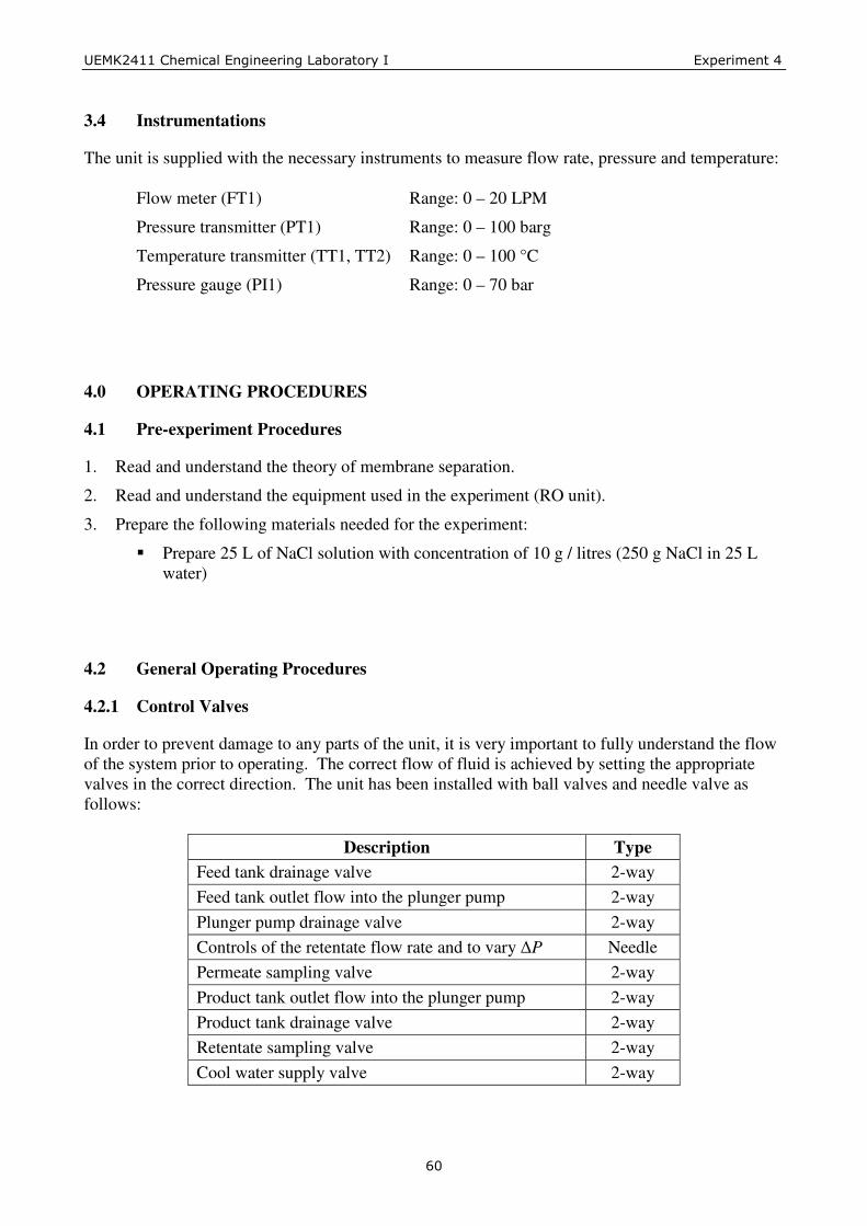
����������� ������� ���� ���������������� � �!"�� �������
� �
3.4 Instrumentations
The unit is supplied with the necessary instruments to measure flow rate, pressure and temperature:
Flow meter (FT1) Range: 0 – 20 LPM
Pressure transmitter (PT1) Range: 0 – 100 barg
Temperature transmitter (TT1, TT2) Range: 0 – 100 °C
Pressure gauge (PI1) Range: 0 – 70 bar
4.0 OPERATING PROCEDURES
4.1 Pre-experiment Procedures
1. Read and understand the theory of membrane separation.
2. Read and understand the equipment used in the experiment (RO unit).
3. Prepare the following materials needed for the experiment:
� Prepare 25 L of NaCl solution with concentration of 10 g / litres (250 g NaCl in 25 L water)
4.2 General Operating Procedures
4.2.1 Control Valves
In order to prevent damage to any parts of the unit, it is very important to fully understand the flow of the system prior to operating. The correct flow of fluid is achieved by setting the appropriate valves in the correct direction. The unit has been installed with ball valves and needle valve as follows:
Description Type Feed tank drainage valve 2-way Feed tank outlet flow into the plunger pump 2-way Plunger pump drainage valve 2-way Controls of the retentate flow rate and to vary �P Needle Permeate sampling valve 2-way Product tank outlet flow into the plunger pump 2-way Product tank drainage valve 2-way Retentate sampling valve 2-way Cool water supply valve 2-way

����������� ������� ���� ���������������� � �!"�� �������
���
4.2.2 Setting the Maximum Working Pressure
1. In order to set the maximum working pressure, close valve V04.
2. Use a wrench to adjust the pressure regulator to a safe low pressure setting by turning the pressure adjuster nut counter-clockwise.
3. Open valve V02 and close valve V01.
4. Ensure that the feed tank is not empty and then switch on the plunger pump (P1).
5. Observe the pressure (PT1) reading next to the pressure regulator. The pressure will rise steadily until it reaches the previously set pressure.
6. Using a wrench, adjust the pressure regulator to obtain the desired maximum working pressure (clockwise to increase pressure; counter-clockwise to decrease pressure).
Note: If the pressure fails to increase or keep-on dropping, there must be air trapped in the membrane system. Shut off the pump and let the air to escape. Ensure that no air is being introduced into the system.
4.2.3 Draining the Leftover
Before flushing the membrane, the leftover liquid has to be completely drained after each session in order to prevent bacterial formation overnight. There are six drainage points provided with the unit. For a complete drainage of the system, open all valves.
5.0 SAFETY PRECAUTIONS
5.1 Pumps Limits
The plunger pump has a working pressure range of 7 to 85 bar. However, to protect the membranes, do not regulate the pressure more than 35 bar.
5.2 Membrane Limits
� The recommended operating pressures of the RO membrane modules are 35 bar. The operating temperature shall not exceed 80°C for RO membranes.
� Operation of membranes at maximum limits of pressure or temperature will affect their subsequent performance at lower temperatures and pressures. In addition, it is not advisable to operate at the limits of temperature and pressure at the same time.
� Test conditions determine the precise retention character.
� The maximum pH range for RO membranes is 1.5 – 12.

����������� ������� ���� ���������������� � �!"�� �������
���
5.3 Control Valves
All valves must be set at the correct positions in order to avoid possible damage to the unit.
5.4 Cleaning Procedures
� After each experiment, drain all process liquid from the process lines, product tank and feed tank.
� Rinse and fill up the feed tank with deionised water.
� Make sure that all valves are set as follows:
Open Close Leave Alone V2, V4 V1, V3, V5, V6, V7, V8 V9
� Set the pressure at 2 – 5 bar and start the plunger pump. Fully open the needle valve (V04) and
let the water flow for about 10 minutes.
� Repeat the above if necessary. Stop the pump and switch off the power supply after all were completed.
6.0 EXPERIMENT
6.1 Experiment 1: Determination of Membrane Resistance, Rm
1. Ensure that the RO membranes (AFC99) are in installed in the membrane module. Ensure that the rubber seals on both ends do not fold. Tighten the screw if necessary and ensure there are no leakages.
2. Follow procedures in Section 4.2.2 to set the maximum working pressure to 35 bar. (Note: for RO filtration never operates the membrane more than 40 bar or more than 80°C)
3. After the maximum pressure is achieved, stop the plunger pump (P1).
4. Fully open valve V02 and V04 and start the plunger pump (P1) again.
5. Connect the cooling coil inlet to cooling water supply and outlet to drain. Open valve V09 to allow water to flow through the cooling coil. (Note: cooling water is used to remove the heat generated from the plunger pump)
6. Set the differential pressure across the membrane to 2 bar by adjusting the needle valve V04. Let the water flow for about 1 minute until the flow rate is stable before taking any reading.
7. Open the sampling valve V08 and drain off the water leftovers from the last experiment. Measures the flow rate of permeate to calculate the flux.
8. Repeat Step 6 and Step 7 with differential pressure of 5, 10, 20 and 30 bar.

����������� ������� ���� ���������������� � �!"�� �������
���
6.2 Experiment 2: Salt Rejection from Water
Experiment 2 is run using the same setup Experiment 1.
1. Ensure that the maximum working pressure is 35 bar.
2. Set the position of the valves as follows:
Open Close Leave Alone V2, V4 V1, V3, V5, V6, V7, V8 V9
3. Fill up the feed tank with of NaCl solution (10 g / litres concentration).
4. Open valve V09 to allow water to flow through the cooling coil. Wait for the temperature to stabilise before taking any readings.
5. Start the plunger pump (P1).
6. Set the inlet pressure to 30 bar by adjusting the needle valve V04. Let the solution flow for about 1 minute until the flow rate is stable before taking any reading
7. While the plunger pump is running, open the bleed screws slowly on both HI and LO side of the differential pressure transmitter to bleed the air trapped inside the system. (Note: the differential pressure reading will be unstable if this step is skipped)
8. Observe and record the increment of conductivity in the feed tank every 2 minute for a duration of 30 minutes.
9. Stop the plunger pump and close valve V02. Pour all the filtrate and retentate back into the feed tank.
10. Repeat the experiment (Step 5 to Step 10) for inlet pressure of 25 bar and 20 bar.
7.0 RESULTS AND DISCUSSIONS
Discuss all your results. The questions below only serve as a guideline. Your discussion should not only limited to these questions.
1. Sketch a schematic diagram, including all valves and sensors/controllers, for the reverse osmosis unit used in the experiment. Label all valves and instruments.
2. Plot the flux, J versus ∆P and calculate the membrane resistance, Rm from the slope of the graph which is equal to )(1 mRµ .
3. For Experiment 2, plot the salt conductivity in the feed tank versus time at different ∆P. Discuss all the findings.