Chris Stiffler, Economist, Colorado Fiscal Institute

1/7/14

COLORADO’S GENUINE

PROGRESS INDICATOR (GPI) A Comprehensive Metric of Economic Well-being in Colorado

from 1960-2011

i

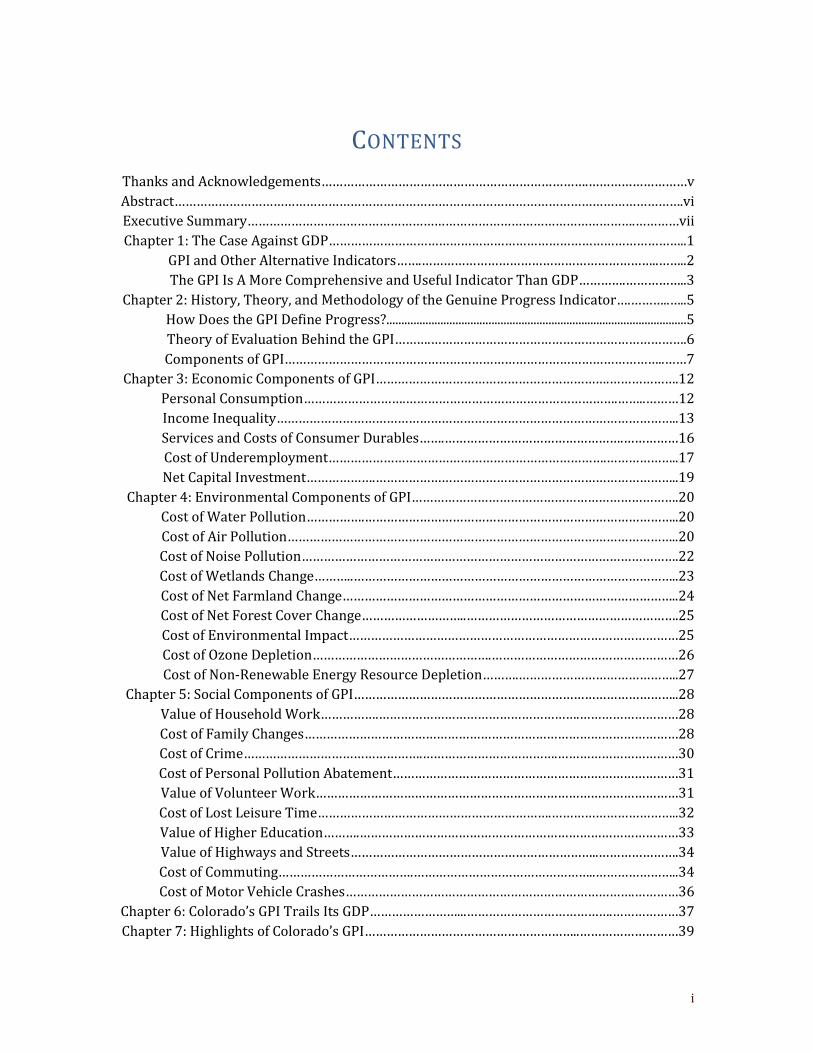
CONTENTS

Thanks and Acknowledgements……………………………………………………………….………………………v

Abstract………………………………………………………………………………………………………………………….vi

Executive Summary…………………………………………………………………………………………….…………vii

Chapter 1: The Case Against GDP……………………………………………………………………………………..1

GPI and Other Alternative Indicators…….………………………………………………………..……..2

The GPI Is A More Comprehensive and Useful Indicator Than GDP………….……………..3

Chapter 2: History, Theory, and Methodology of the Genuine Progress Indicator….………..…..5

How Does the GPI Define Progress?....................................................................................................5

Theory of Evaluation Behind the GPI……….…………………………………………………………….6

Components of GPI…………………………………………………………………………………………..……7

Chapter 3: Economic Components of GPI……………………………………………………….……………….12

Personal Consumption……………………….………………………………………………….……..………12

Income Inequality………………………………………………………………………………………………..13

Services and Costs of Consumer Durables…….………………………………………….……………16

Cost of Underemployment………………………………………………………………….………………..17

Net Capital Investment……………….………………………………………………………………………..19

Chapter 4: Environmental Components of GPI……………………………………………………………….20

Cost of Water Pollution…………….…………………………………………………………………………..20

Cost of Air Pollution……………………………………………………………………………………………..20

Cost of Noise Pollution………………………………………………………………………………………….22

Cost of Wetlands Change………..……………………………………………………………………………..23

Cost of Net Farmland Change………………………………………………………………………………..24

Cost of Net Forest Cover Change………………………..………………………………………………….25

Cost of Environmental Impact………………………………………………………………………………25

Cost of Ozone Depletion………………………………………….……………………………………………26

Cost of Non-Renewable Energy Resource Depletion……….……………………………………..27

Chapter 5: Social Components of GPI……………………………………………………………………………..28

Value of Household Work…………….……………………………………………….………………………28

Cost of Family Changes…………………………………………………………………………………………28

Cost of Crime………………………………………….……………………………….……………………………30

Cost of Personal Pollution Abatement……………………………………………………………………31

Value of Volunteer Work………………………………………………………………………………………31

Cost of Lost Leisure Time……………………………………………………….……………………………..32

Value of Higher Education……….……………………………………………………………………………33

Value of Highways and Streets…………………………………………………………..………………….34

Cost of Commuting……………………………….…………………………………………..…………………..34

Cost of Motor Vehicle Crashes…………………………………………………………………….…………36

Chapter 6: Colorado’s GPI Trails Its GDP……………………...………………………………….………………37

Chapter 7: Highlights of Colorado’s GPI…………………………………………………..………………………39

ii

A Look at Economic Well-being……………………………………………………………….…………..39

Where Colorado has had declining economic well-being……….……………40

Where Colorado has improved economic well-being………..…..…………….40

A Look at Environmental Well-being………………………………………………….….…………….41

Where Colorado Has had declining environmental well-being….…………42

Where Colorado has improved environmental well-being….…….…………42

A Look at Social Well-being…………………………………………………………………………………43

Where Colorado has had declining social well-being…………...………………44

Where Colorado has improved social well-being…………………………………44

References……………………………………………………………………………………………………………………45

Appendix A: Detailed Methods of Colorado’s GPI…………………………………….………………………51

Appendix B: Detailed CO-GPI Results………………………………………………………………………………61

iii

FIGURES

Figure 1. Economic, Social, and Environmental Components of the CO-GPI………………………..ix

Figure 2. Values and Costs of CO-GPI in 2011 (millions of 2000 USD)……………..…………………..x

Figure 3. Developing GPI from GDP……………………………………………………………………………….….3

Figure 4. Growing Inequality Reduces Economic Well-Being…………………………………………...15

Figure 5. Growing Inequality……………………………………………………………………………………….....15

Figure 6. Cost of Income Inequality Per Capita………………………………………………………………..16

Figure 7. Net Services of Consumer Durables Per Capita……………………………………………….....17

Figure 8. Underemployment Rate in Colorado………………………………………………………………...18

Figure 9. Cost of Underemployment Per Capita…………………………………………………………….....18

Figure 10. Value of Net Capital Investment Per Capita………………………………………………….….19

Figure 11. Cost of Air Pollution Per Capita………………………………………………………………………21

Figure 12. Cost of Noise Pollution Per Capita…………………………………………………………………..22

Figure 13. Cost of Net Wetland Change Per Capita………………………………………………………..….23

Figure 14. Cost of Net Farmland Change Per Capita…………………………………………………………24

Figure 15. Cost of Net Forest Cover Change Per Capita…………………………………………………….25

Figure 16. Cost of Environmental Impact Per Capita………………………………………………………..26

Figure 17. Cost of Ozone Depletion Per Capita…………………………………………………………………26

Figure 18. Cost of Nonrenewable Energy Resource Depletion Per Capita………………………....27

Figure 19. Value of Housework Per Capita…………………………………………………………………...….28

Figure 20. Cost of Divorce Per Capita…………………………………………..………………………………….29

Figure 21. Cost of TV Watching Per Capita………………………………………………………………………29

Figure 22. Cost of Crime Per Capita………………………………………………………………………………...30

Figure 23. Cost of Personal Pollution Abatement Per Capita…………………………………………….31

Figure 24. Value of Volunteer Work Per Capita………………………………………………………………..32

Figure 25. Lost Leisure Per Unconstrained Worker (Hours)……………………………...……………..32

Figure 26. Cost of Lost Leisure Time Per Capita………………………………………...…………………….33

Figure 27. Value of Higher Education Per Capita………………………………………………………….….33

Figure 28. Services of Highways and Streets Per Capita………………………………………………..….34

Figure 29. Cost of Commuting Per Capita………………………………………………………………………..35

Figure 30. Cost of Motor Vehicle Crashes Per Capita………………………………………………………..36

Figure 31. GPI vs. GDP Per Capita…………………………………………………………………………………...37

Figure 32. CO-GPI and Components Per Capita………………….……………………….……………………38

Figure 33. Values and Costs of CO-GPI in 2011………………………………….……………………………..38

Figure 34. Economic Components of CO-GPI Per Capita……………………………………...……………39

Figure 35. Economic Components of CO-GPI by Decade Per Capita……………………………..……39

Figure 36. Environmental Components of CO-GPI Per Capita……………….…………………………..41

Figure 37. Environmental Components of GO-GPI by Decade…………………………………………...41

Figure 38. Social Components of CO-GPI by Decade Per Capita………………..……………………….43

iv

TABLES

Table 1: A New Paradigm to Measure Progress……………………………….……………….….…………….6

Table 2: Components and Methods of Calculation for Colorado’s GPI………….……….………..……8

Table 3: Derivation of Personal Consumption Per Capita………………………………………...……….12

Table 4: Where Colorado Ranks: Personal Income Per Capita……………………………………….….13

Table 5: Adjusting Personal Consumption for Income Inequality……………..………………..……..14

Table 6: The Cost of Water Pollution in Colorado……………………………………………………...……..20

Table 7: Coloradans Living in Cities……………………………………………………………………......………22

Table 8: Cost of Lost Farmland in Colorado……………………………………………………………………..24

v

THANKS AND ACKNOWLEDGEMENTS

We owe much gratitude to the researchers, colleagues and partners who helped get this

project moving.

That includes Demos and Lew Daly for keeping the GPI momentum going stronger.

We need to give special thanks to Sean McGuire, Kenneth Bagstad and John Talberth.

We are also indebted to all the scholars who designed Maryland’s GPI model, which was the

scaffolding the Colorado GPI is modeled after. As well as the scholars behind the Utah GPI

report which helped provide guidance adopting the GPI model for a mountain-region state.

Thanks to a few other colleagues that assisted in finding Colorado-specific data for the GPI

and for giving us feedback and collaboration:

Kyle Fritz at the National Transit Database

John Elias at the Regional Transportation District (RTD).

Joan Pinamont, CDOT Librarian

Josh Drukenbrod, statistician at EPA

Dr. Paula Cole and her University of Denver classes

Sarah Wilhelm

vi

ABSTRACT

This study calculates a new, more comprehensive metric to measuring economic well-being

in Colorado known as the Genuine Progress Indicator (GPI). The standard proxy for

measuring a state’s economic well-being has been GDP (Gross Domestic Product), even

though it was never intended to be a proxy for economic well-being. The GDP accounting

method adds up all monetary transactions that occur in a given year. Being a broad measure

of economic activity, GDP does not make any distinction between these activities, thereby

counting “defensive expenditures” or “regrettable” transactions as positive that don’t add to

economic well-being. GPI also omits environmental externalities and ignores negative social

conditions ranging from family breakdown to crime as well as positives like volunteerism,

household labor and economic benefits from farms and forests.

The new metric, GPI, gets closer to the reality of economic well-being by establishing an

accounting method that subtracts and adds factors that contribute and detract from

Coloradans’ economic welfare.

GPI starts with a proxy for material welfare — the amount of goods and services Coloradans

themselves buy each year — known as personal consumption expenditures. This is then

adjusted for income inequality, accounting for the fact that added consumption beyond the

point of meeting basic needs provides increasingly less economic satisfaction. With adjusted

personal consumption as the baseline, GPI adds the monetary value of activities that add to

economic well-being but are not counted in the standard GDP framework. These include

things like household labor, volunteer labor and benefits of higher education. GPI then

subtracts the monetary cost of the expenditures that we incur to protect the depletion of

our natural and social capital. These include things like the cost of auto accidents, costs of

crime, lost leisure time and pollution. Twenty-four factors are included to generate the

Colorado GPI for the years 1960-2011.

vii

EXECUTIVE SUMMARY

Coloradans these days are working longer for less money, spending more time commuting

to work and fewer hours with family. At the same time, there are more "underemployed"

Coloradans than ever before. And the gap between the wealthiest and the poorest people in

our state is the biggest it has been in at least 50 years.

That doesn’t mean the Colorado economy hasn’t grown steadily for the last several decades,

however. If you just look at the state’s Gross Domestic Product, or GDP, it appears Colorado

has been doing better economically for the last half century. But is GDP really the right way

to determine if most Coloradans themselves have experienced economic progress?

That’s where GPI, or the Genuine Progress Indicator, comes in. GPI is a measure of economic

well-being that is increasingly being used to gauge economic progress. GPI measures in

economic terms what GDP can't — whether people's lives are improving.

If you were attempting to see how successful a business is, you wouldn't look only at gross

revenues. You'd also look at expenses, things on the negative side of the ledger like payroll,

capital costs, insurance, utilities and debt service. And if you were taking a smart look, you

wouldn't just examine the things with obvious dollar amounts attached to them. You'd also

measure things that were less visible but that still came with real costs attached, things like

opportunity costs from certain business decisions. You’d probably also consider how

sustainable a company’s practices are.

In the same way, when you look at the economic well-being of a nation, or a state, you can't

just look at the sum total of all economic transactions as the measure of how well off its

residents are. But that's basically what GDP does. Even though GDP was never intended to

measure economic well-being, it's commonly looked at that way. So, for example, if a house

that has burned to the ground gets rebuilt, the money spent reconstructing that house is

counted as a positive under GDP, even though you're just rebuilding the same house. You're

no better off than you were before your house burned down.

For the last few decades, economists have been developing a measure that more accurately

and thoughtfully addresses the question of whether the economic well-being of a

population has increased or not. This more recent form of measurement, the Genuine

Progress Indicator, has been used in several other states including Maryland, Utah,

Vermont, Ohio and Minnesota, and there are efforts afoot in other states to measure GPI.

This study calculates GPI in Colorado using 24 recognized indicators that balance positive

economic factors — things like net capital investment, hours spent volunteering, the value

of higher education, highways and streets and the value of consumer durables —with

negative ones, like the costs of crime, underemployment, pollution and income inequality.

viii

What the study shows is that while Colorado's per capita GDP has tripled since 1960, GPI,

expressed as a dollar figure per capita, has trailed behind significantly.

GPI is a more useful metric than GDP. One of the biggest limitations with GDP as a measure

of economic well-being is that it counts “regrettable” or “defensive” expenditures the same

way it counts other spending, even though these expenditures are often made simply to

mitigate the way we live.

For example, more money that is spent on driving to work merely adds to GDP even though

it also results in more time spent in traffic, which reduces time available to be spent on

work, leisure or family. More money spent cleaning up pollution increases GDP even though

this is merely a cost of mitigating the negative effects of another economic activity. Under

GDP, if the size of the economy increases dramatically because a small number of people

have become exceptionally wealthy, this is counted as a positive, even though it may mean

staggering income inequality that leads to a lack of social cohesion and decreased

consumption, the engine that drives the entire economy.

Under the Genuine Progress Indicator, these negative effects are assigned a dollar value that

is subtracted from total personal consumption, resulting in a per capita sum that is more

reflective of economic progress or well-being. In addition, GPI adds in certain positive

factors to the economy that GDP does not account for, such as the value of volunteer hours,

household labor and higher education.

GPI is calculated using three sets of indicators: economic, social and environmental. Some

indicators add value while others subtract value.

Economic indicators include things such as the costs of underemployment and income

inequality and the value of personal consumption. The economic components have the

largest impact on GPI, making up a net positive of $116 billion.

Social indicators are things such as the value of volunteer hours and the costs of lost leisure

time, crime and divorce. The social elements of the GPI add a net positive to well-being of

$23 billion, the largest components being household work and the value of higher

education.

Environmental indicators include things such as the costs of pollution, resource depletion

and the loss of farmland, wetlands and forest cover. These environmental components

contribute a net loss to Colorado’s GPI by deducting $35.3 billion. More than half of the costs

of environmental damage come from depletion of non-renewable energy sources.

ix

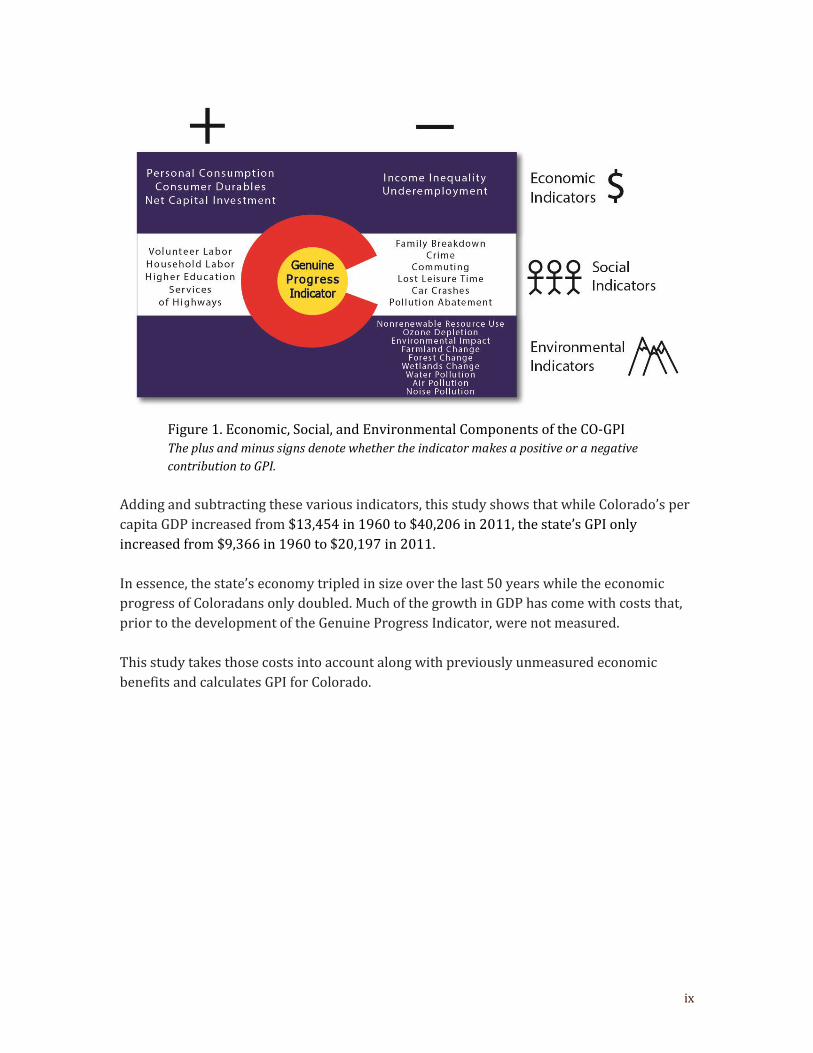
Figure 1. Economic, Social, and Environmental Components of the CO-GPI The plus and minus signs denote whether the indicator makes a positive or a negative

contribution to GPI.

Adding and subtracting these various indicators, this study shows that while Colorado’s per

capita GDP increased from $13,454 in 1960 to $40,206 in 2011, the state’s GPI only

increased from $9,366 in 1960 to $20,197 in 2011.

In essence, the state’s economy tripled in size over the last 50 years while the economic

progress of Coloradans only doubled. Much of the growth in GDP has come with costs that,

prior to the development of the Genuine Progress Indicator, were not measured.

This study takes those costs into account along with previously unmeasured economic

benefits and calculates GPI for Colorado.

x

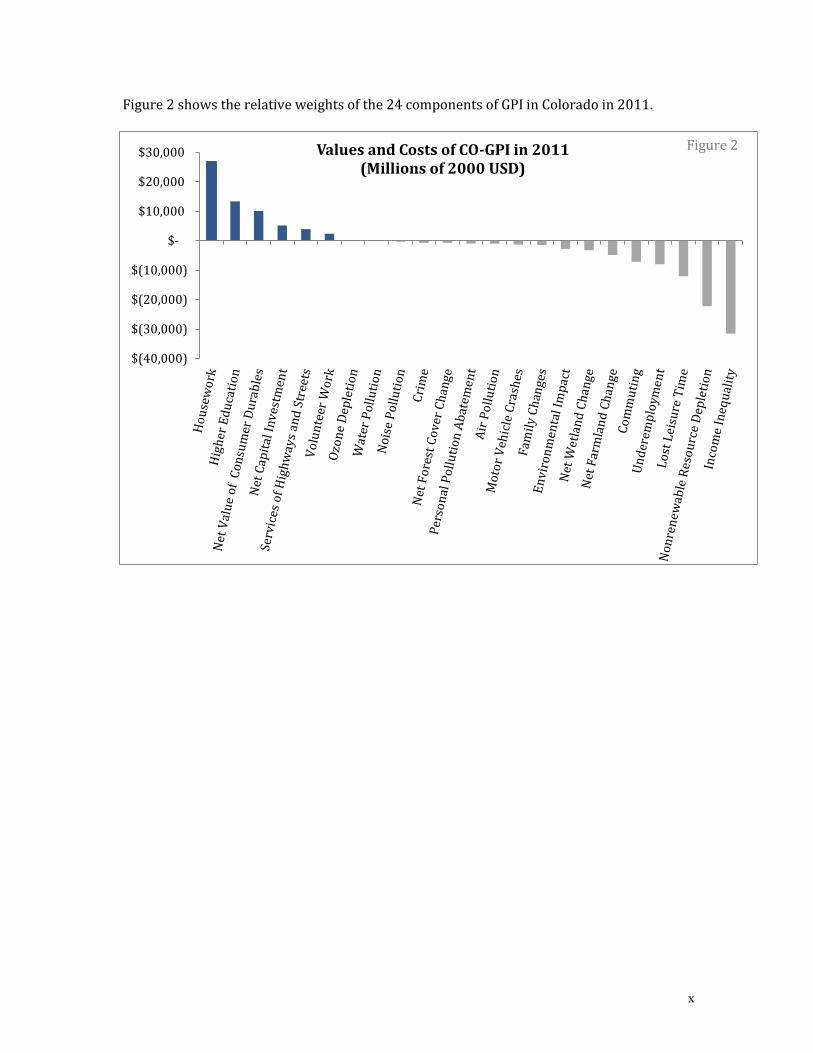
Figure 2 shows the relative weights of the 24 components of GPI in Colorado in 2011.

$(40,000)

$(30,000)

$(20,000)

$(10,000)

$-

$10,000

$20,000

$30,000 Values and Costs of CO-GPI in 2011(Millions of 2000 USD)

Figure 2

1

CHAPTER 1: THE CASE AGAINST GDP

Most economic and budget policy decisions are viewed through the lens of economic

growth, measured by GDP, or Gross Domestic Product. Behind those decisions lies the

assumption that well-being is directly related to economic growth.

Looking at a standard measure of economic activity in Colorado, such as GDP, indicates

there has been strong growth both in total value and in per capita terms the last several

decades. In fact, real GDP per capita tripled in Colorado from 1960 to 2011. But does that

really mean that the typical Coloradan is three times better off today than he or she was in

1960? While the consumption of goods and services has continually risen, income

inequality has risen, average real hourly wages have declined and quality time spent with

family has eroded. GDP has created a false illusion that the state is getting richer and the

state’s well-being is improving at a faster rate than it really is.

Everything is three times better today than in 1960, at least according to the default

yardstick of economic well-being, GDP.

Although it has become a proxy for progress, GDP has many limitations that prevent the

metric from correlating closely with economic well-being. Since its introduction, economists

have warned that considering GDP a general indicator of well-being was dangerous

(Kuznets, 1934, Kuznets et al., 1941).

GDP is a tally of all monetary exchanges that occur in a given year; it doesn’t differentiate

between economic purchases that add to our well-being and ones that undermine it. For

example, rebuilding homes destroyed by forest fires actually add to GDP since all that

money is spent in new construction. But this construction only gets us back to where we

were before the fire and also diverts the goods and services used on reconstruction away

from investments that would improve well-being in the future.

GDP also counts, as a positive, the expenditures made to protect people from the side effects

of current and past economic activities. These dollars do not add to well-being; they only

prevent its deterioration. Other GPI studies call these expenditures “defensive” since they

are expenditures that “we have to make to protect ourselves from the unwanted

consequences of the production and consumption of other goods by other people” (Daly and

Farley 2004). Such an example would be the cost of disposing of garbage; such a purchase

doesn’t add to well-being but is necessary.

GDP does not consider the distribution of growth. If the size of the economy doubled but all

that wealth went to only a handful of individuals, would the economic well-being of the

typical Colorado family improve? Under the GDP accounting system, it would.

GDP does not take into account non-market activities like commuting time or lost leisure

time. All Coloradans could suddenly decide to work 80-hour weeks and dramatically boost

the number of dollars we earn and spend, although we’d be sacrificing 40 hours we would

2

have been spending with family and friends. The current GDP framework doesn’t take into

account lost time with families or lost leisure. Working 80-hour weeks would only be a

positive.

GDP doesn’t account for non-market services of the environment or the individual. All the

hours Coloradans volunteer are not counted in GDP nor are the hours of household labor

Coloradans perform every year.

GDP tells us nothing about sustainability. GDP counts the consumption of natural resources

as strictly positive. So we could deplete all Colorado’s mines and divert every drop of water

to agriculture in one year to dramatically boost our state GDP, but it doesn’t tell us whether

production and consumption involve unsustainable activities. GDP doesn’t account for

negative externalities created by the way we live. So the damage from pollution is ignored.

Given the many limitations of GDP acting as a pure indicator of economic well-being, GDP

can be viewed as a business reporting only total revenue while neglecting to subtract

expenses or depreciation of company equipment. Another way to view the limitations of

GDP is to think of GDP as a measure of economic quantity, not economic quality or welfare

(Posner, 2010).

Prioritizing economic well-being instead of economic growth requires an alternative

measure to GDP accounting.

GPI and Other Alternative Indicators

The GPI is an objective, composite index just like GDP. The difference is that GPI makes

corrections to the existing GDP framework. It uses data sets about factors ranging from

commute time, to volunteer hours, to number of college graduates, to acreage of forest land.

Each indicator is translated into an objective dollar amount. With every factor in dollar

terms, economic, social and environmental factors can be aggregated. For example, an hour

spent volunteering is worth an hour’s pay at Colorado’s average volunteer wage rate. Each

incident of breaking-and-entering crime costs $1,513 — the average of all B-and-E incidents

— and is subtracted from the GPI. Having all of the components of GPI in dollar terms

allows trade-offs to be shown — so an increase in a cost like pollution could be offset by an

increase in a benefit like personal consumption.

The GPI should not be confused with subjective measures of happiness. We make the

distinction between economic well-being and happiness here. The GPI does not directly

measure happiness. It shows the potential for community well-being. The GPI is best

thought of as a more comprehensive form of measuring economic progress that measures

the total economy. The GPI does something completely different than indices that look at

individuals. The methodology here follows what previous GPI studies have calculated.

There are many other indicators that keep track of changes in poverty, the economy,

housing, education, health, crime and transportation. The GPI does not supplant these

3

indicators, it simply contributes to the analysis of community well-being by offering a single

numeric metric that incorporates a wide range of indicators.

The GPI is a More Comprehensive and Useful Indicator Than GDP

The Genuine Progress Indicator (GPI) provides a more comprehensive measure that

attempts to correct many of the flaws of GDP accounting. At the most basic level, the GPI

adopts an economic accounting system that starts with something like GDP but then adds

those factors that contribute to economic well-being and subtracts the monetary value of

factors that detract from it that are omitted in the GDP framework. It is one of the first

alternatives to GDP vetted by the scientific community and used by governments to show

economic welfare (Talberth et al., 2007).

The GPI attempts to equate dollars to economic well-being. All the dollars in GPI add to

economic well-being because the “defensive” dollars are subtracted out. The dollars earned

from over-utilizing resources are subtracted since they won’t be around in the future. The

dollar value of factors that add to our economic well-being but are currently omitted by GDP

are added back in. The value of the negative externalities like pollution that aren’t counted

in GDP are subtracted.

Figure 3. Developing GPI from GDP

4

The overarching question that the GPI sets out to answer is: “Has the economic growth in

Colorado over the past five decades led to social, economic and environmental progress?”

Adopting a GPI accounting metric in Colorado is meant to accomplish a number of goals:

Identify opportunities for Coloradans to improve their economic well-

being.

Show how much “defensive” spending (expenditures that do not add

to well-being but merely prevent its erosion) Coloradans undertake

as a result of the way we live and consume.

Assess whether economic well-being is improving and show the

trends over time.

Provide Colorado decision makers with a more comprehensive

method to assess the full effects of public policy and budget decisions.

Allow policy-makers to examine the trade-offs of allocating and using

particular resources.

5

CHAPTER 2: HISTORY, THEORY, AND METHODOLOGY OF

THE GENUINE PROGRESS INDICATOR (GPI)

The current GPI metric is a product of evolution since the first alternative was published in

the 1970s. In 1972, as one of the earliest attempts to correct for the limitations of GDP,

James Tobin and William Nordhaus created the Measure of Economic Welfare (MEW),

which makes adjustments to GDP for typically unaccounted-for economic and social factors.

The first adjustment was to subtract out the money spent on items that didn’t add to well-

being that were counted as positives in GDP. “Since GDP is a measure of production rather

than of welfare, they count many activities that are evidently not directly sources of utility

themselves but are regrettable necessary inputs to activities that may yield activity.”

(Nordhaus and Tobin, 1972). Next, values of leisure and household activities were added in.

Adjustments were made for capital accumulation in order to account for the costs of

depletion of capacity to yield future production. Finally, an imputed value of urban

disamenities, or unfavorable qualities of city life — such as traffic congestion, pollution and

crime — was backed out because “some portion of higher earnings of urban residents may

simply be compensation for the disamenities of urban life and work” (Nordhaus and Tobin,

1972, page 12).

Another alternative index came out in the early 1980s known as the Index of the Economic

Aspects of Welfare (Zolotas, 1981). It differed widely from the MEW by focusing on the

current flow of goods and services and largely ignoring capital accumulation and

sustainability. Both studies, despite their different methodologies, provided early evidence

of the gap between GDP and well-being and quantitatively showing that more and more

economic activity may be self-canceling from an overall well-being standpoint (Posner,

2010).

Then in the late 1980s, Herman Daly and Clifford Cobb developed the Index of Sustainable

Economic Welfare (ISEW), which built upon the MEW but also included environmental

costs. In the 1990s, the ISEW was adjusted by Cobb, Rixford, Halstead and Rowe. They

referred to their product for the first time as the GPI.

There are a handful of states that have created local-level GPI studies: Maryland (Maryland

Genuine Progress Indicator 2010, Posner 2010); Minnesota (Minnesota Planning Agency

2000); California (Bay Area Genuine Progress Indicator 2006); Ohio (Bagstad and Shammin

2012); Utah (Berik and Gaddis 2011); Vermont (Costanza et al., 2004 and Bagstad and

Ceroni, 2007); and Hawaii (Hawaii State Environmental Council 2013).

How Does the GPI Define Progress?

How we define progress determines how and where society allocates its collective efforts.

The notion that economic growth represents general societal progress causes many

problems. Defining progress based solely on economic growth in GDP has led to a situation

6

where high economic growth rates are achieved at the expense of other forms of progress,

such as mental and physical well-being, clean air and water or cohesive communities. The GPI defines progress differently than the standard economic idea of progress. The GPI

adopts the notion of progress from a relatively new branch of economics: ecological

economics, which emphasizes the goals of achieving optimal scale, fair distribution and

efficient allocation of resources instead of simple economic growth (Daly and Farley, 2004).

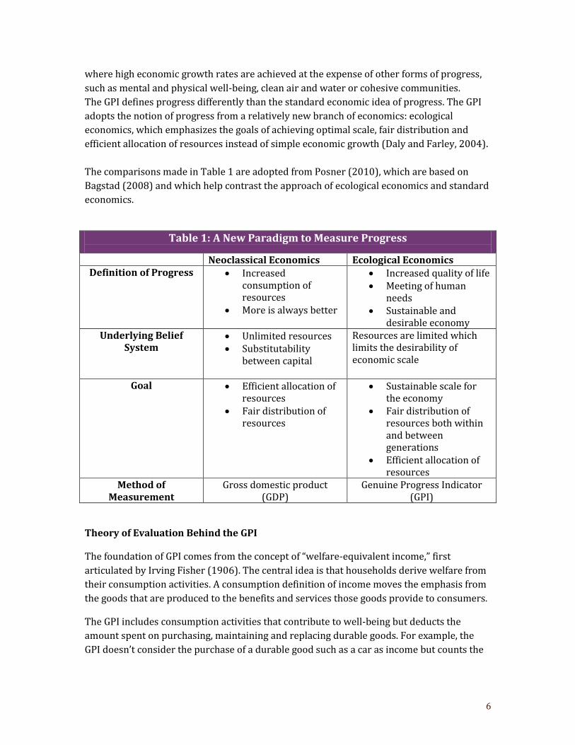
The comparisons made in Table 1 are adopted from Posner (2010), which are based on

Bagstad (2008) and which help contrast the approach of ecological economics and standard

economics.

Table 1: A New Paradigm to Measure Progress

Neoclassical Economics Ecological Economics Definition of Progress Increased

consumption of resources

More is always better

Increased quality of life Meeting of human

needs Sustainable and

desirable economy Underlying Belief

System Unlimited resources Substitutability

between capital

Resources are limited which limits the desirability of economic scale

Goal Efficient allocation of resources

Fair distribution of resources

Sustainable scale for the economy

Fair distribution of resources both within and between generations

Efficient allocation of resources

Method of Measurement

Gross domestic product (GDP)

Genuine Progress Indicator (GPI)

Theory of Evaluation Behind the GPI

The foundation of GPI comes from the concept of “welfare-equivalent income,” first

articulated by Irving Fisher (1906). The central idea is that households derive welfare from

their consumption activities. A consumption definition of income moves the emphasis from

the goods that are produced to the benefits and services those goods provide to consumers.

The GPI includes consumption activities that contribute to well-being but deducts the

amount spent on purchasing, maintaining and replacing durable goods. For example, the

GPI doesn’t consider the purchase of a durable good such as a car as income but counts the

7

benefits that the car gives over its lifetime. It’s best to think of “welfare-equivalent income”

in the net sense (Lawn, 2003).

The GPI model is based on the principle of non-declining stock of built and natural capital.

This stock of capital must be available for future generations. So deductions are made in the

GPI model to account for declining natural and built capital.

The philosophy behind the environmental components of the GPI is based on the principal

of “strong sustainability” (Lawn 2003, Talberth 2007, Baumgartner and Quaas 2009). This

means that there is a limit to the extent to which built capital — buildings, bridges and

other manmade objects — can substitute for depleted natural capital, resources such as

timber, farmland and water. Thus, to keep the stock of natural capital intact, the cost of

natural resource depletion must be factored into an evaluation of well-being (Berik and

Gaddis, 2011). The current GPI actually measures “weak sustainability” because we can be

losing environmental or social capital if we’re growing built capital at a fast enough rate.

This is an ongoing critique of the GPI that the scientific community is working out.

The social domain of the GPI is based on the notion that the quality of social life is integral

to well-being and must be sustained into the future. Therefore, GPI values the many unpaid

activities that sustain and build families and communities.

Components of GPI

The GPI is measured in dollars. The GPI model aggregates the various indicators into a

single number with dollars as the denominator. Hence, the model must assign monetary

units to environmental and social indicators (the economic indicators are mostly already

captured in dollars). For example, an acre of farmland is assigned a dollar value to represent

what that acre contributes to society. If that acre is lost, the value of that acre subtracts from

GPI.

Assigning a dollar value to non-market items is inherently challenging, but is necessary to

establishing relative worth among resources managed by society (Hawaii State

Environmental Council, 2013). The model used the best possible estimates from peer-

reviewed valuation studies.

Since GPI is reported in a single number for each year, it makes communicating with the

public much simpler and it can be compared with other metrics more readily. The GPI can

also be broken down into its components and analyzed in depth. For instance,

environmental groups can look at the sub-component environmental indicator which can

further be scrutinized down to the forest indicator.

The GPI framework starts with personal consumption expenditures — which can be

thought of simply as the amount of goods and services Coloradans themselves buy each

year. This is then adjusted for income inequality. With adjusted personal consumption as

the baseline, GPI adds the monetary value of activities that add to economic well-being but

are not counted in the standard GDP framework. These include things like: household labor,

8

volunteer labor and benefits of higher education. GPI then subtracts the monetary cost of

the expenditures that we incur to protect the depletion of our natural and social capital.

These include things like: cost of auto-accidents, costs of crime, lost leisure time and

pollution. It also subtracts the money Coloradans spent on items that must be spent to abate

the negative outcomes that result from the way we live and consume. For example, money

spent to dispose of our waste.

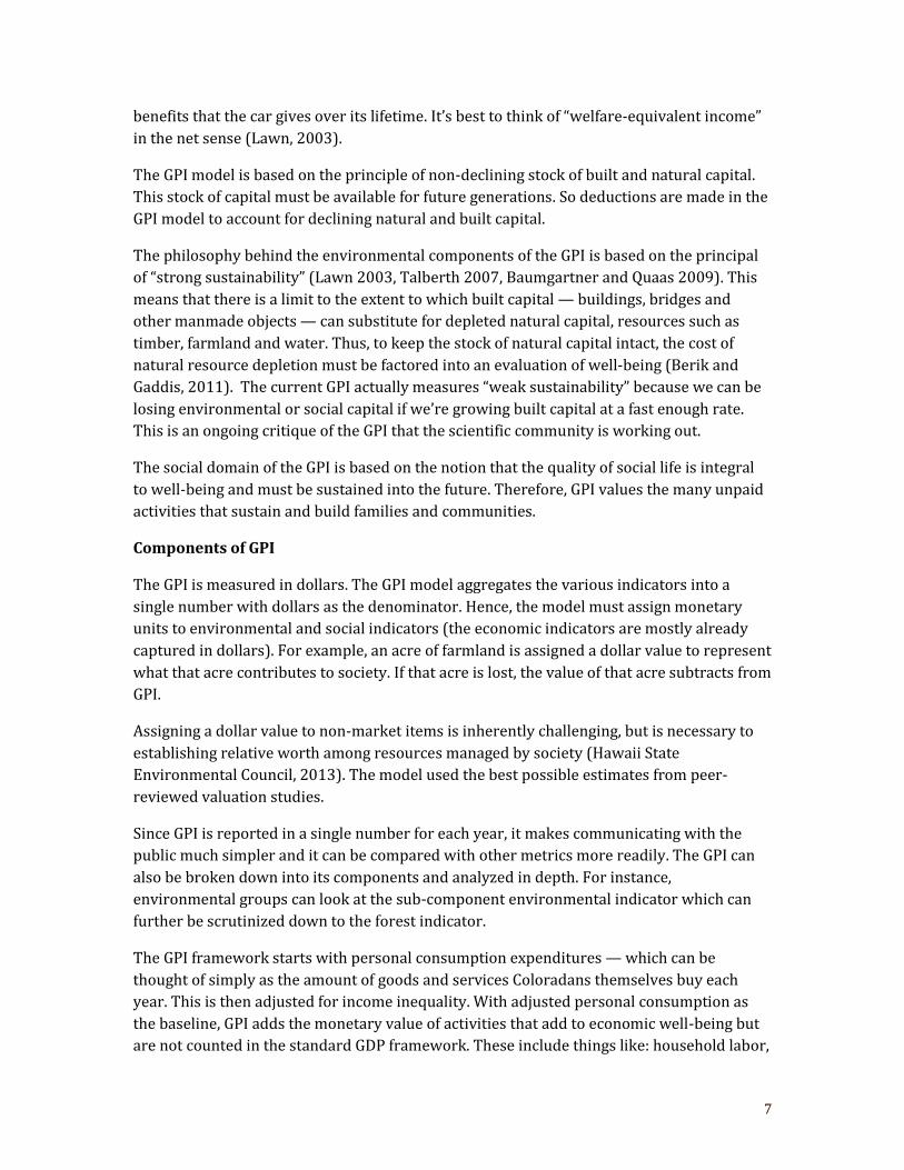
These 24 indicators, in Table 2, fall into three categories: economic, environmental and

social.

Table 2: Components and Methods of Calculation for Colorado’s GPI

Indicator

Impact on

Well-Being

Description

Formula

A. Personal Consumption Expenditure

+ baseline Starting point for GPI. Personal Income

multiplied by the national ratio of consumption to income spending.

B. Income Distribution + or - Severe income

inequality has social and economic costs not captured by the GDP.

Gini coefficient in year divided by Gini coefficient at baseline low value multiplied by 100.

C. Inequality-adjusted Consumption Expenditure

Becomes the baseline from which other GPI components are added or deducted.

Row A divided by Row B.

D. Benefits of Consumer Durables + Estimates the services

provided by household equipment, which is a more accurate measure of value that just the money spent on such long-term items.

20 percent of stock of consumer durables.

E. Cost of Consumer Durables - The price of durables is

subtracted to avoid double counting the value in their services and personal consumption.

Personal Income multiplied by national percentage of spending on consumer durables.

F. Underemployment - Involuntary part-time

workers, discouraged workers and the chronically unemployed represent reduced well-being.

Underemployed persons multiplied by unprovided work hours per constrained worker multiplied by average hourly wage.

9

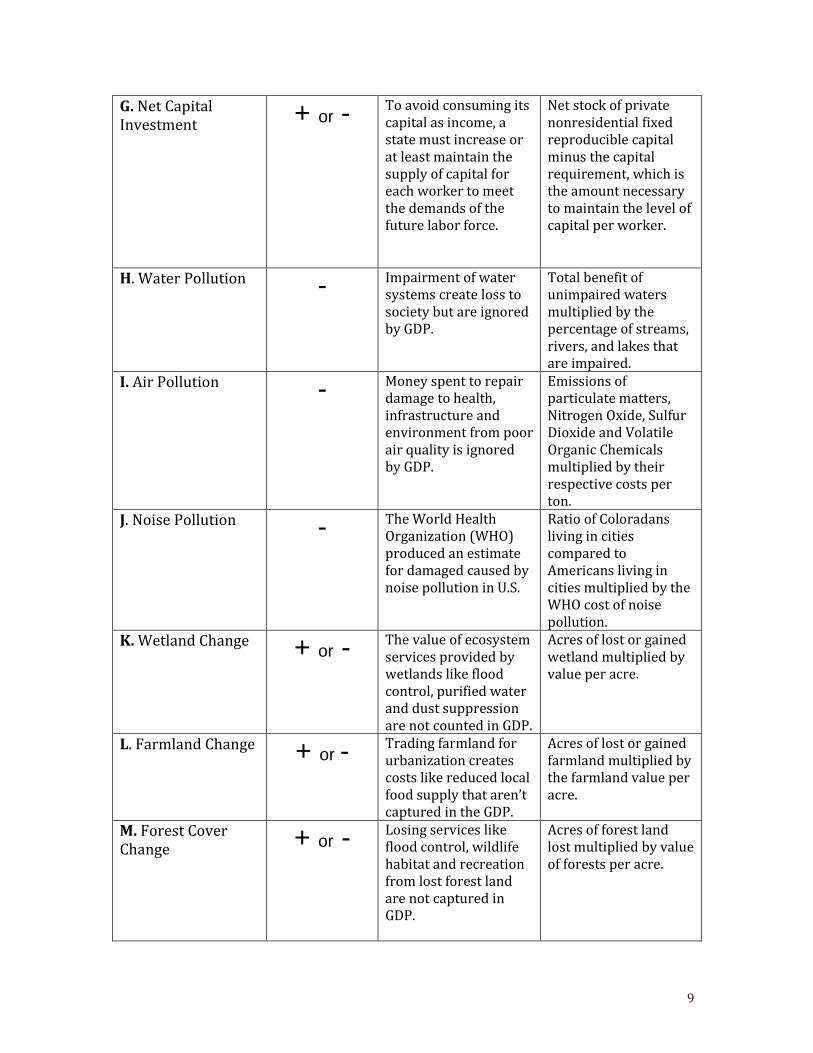
G. Net Capital Investment + or - To avoid consuming its

capital as income, a state must increase or at least maintain the supply of capital for each worker to meet the demands of the future labor force.

Net stock of private nonresidential fixed reproducible capital minus the capital requirement, which is the amount necessary to maintain the level of capital per worker.

H. Water Pollution - Impairment of water systems create loss to society but are ignored by GDP.

Total benefit of unimpaired waters multiplied by the percentage of streams, rivers, and lakes that are impaired.

I. Air Pollution - Money spent to repair damage to health, infrastructure and environment from poor air quality is ignored by GDP.

Emissions of particulate matters, Nitrogen Oxide, Sulfur Dioxide and Volatile Organic Chemicals multiplied by their respective costs per ton.

J. Noise Pollution - The World Health Organization (WHO) produced an estimate for damaged caused by noise pollution in U.S.

Ratio of Coloradans living in cities compared to Americans living in cities multiplied by the WHO cost of noise pollution.

K. Wetland Change + or - The value of ecosystem services provided by wetlands like flood control, purified water and dust suppression are not counted in GDP.

Acres of lost or gained wetland multiplied by value per acre.

L. Farmland Change + or - Trading farmland for urbanization creates costs like reduced local food supply that aren’t captured in the GDP.

Acres of lost or gained farmland multiplied by the farmland value per acre.

M. Forest Cover Change + or - Losing services like

flood control, wildlife habitat and recreation from lost forest land are not captured in GDP.

Acres of forest land lost multiplied by value of forests per acre.

10

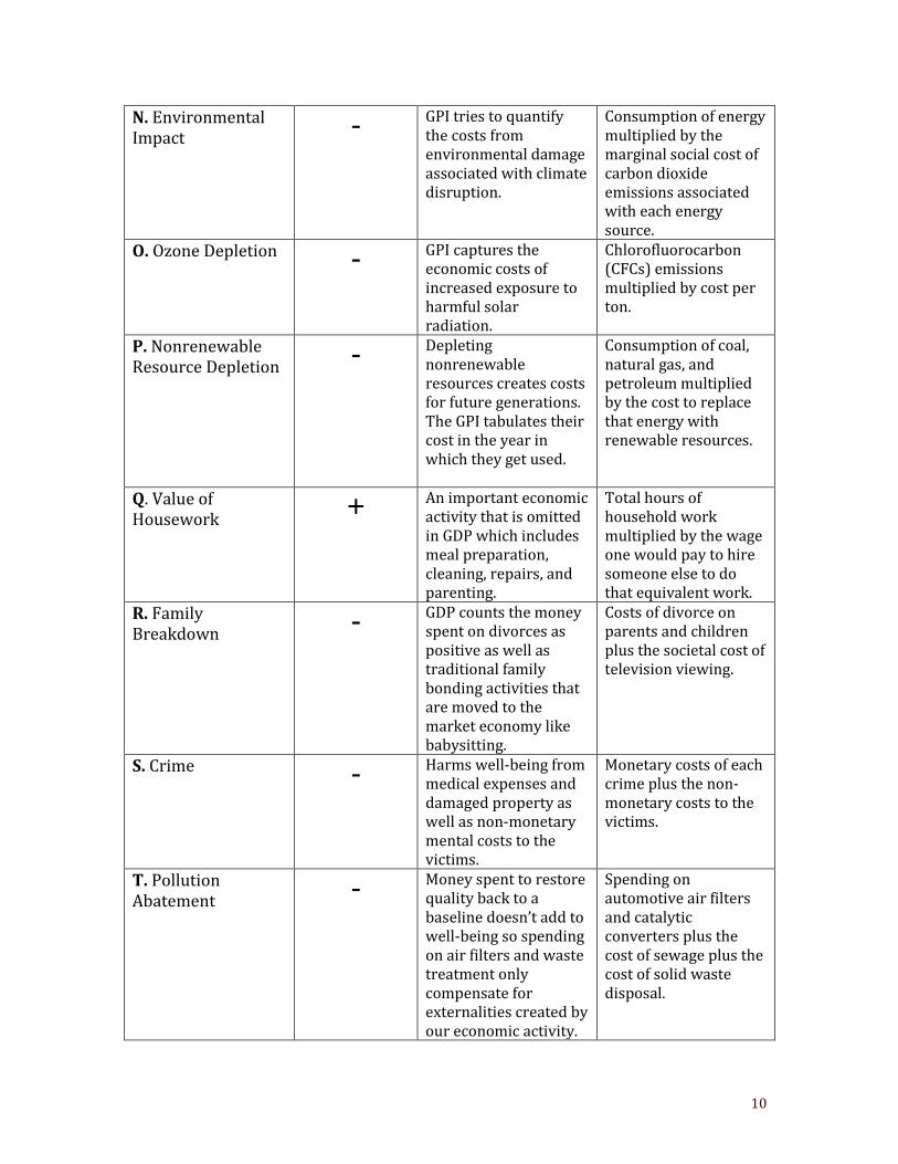
N. Environmental Impact - GPI tries to quantify

the costs from environmental damage associated with climate disruption.

Consumption of energy multiplied by the marginal social cost of carbon dioxide emissions associated with each energy source.

O. Ozone Depletion - GPI captures the economic costs of increased exposure to harmful solar radiation.

Chlorofluorocarbon (CFCs) emissions multiplied by cost per ton.

P. Nonrenewable Resource Depletion - Depleting

nonrenewable resources creates costs for future generations. The GPI tabulates their cost in the year in which they get used.

Consumption of coal, natural gas, and petroleum multiplied by the cost to replace that energy with renewable resources.

Q. Value of Housework + An important economic

activity that is omitted in GDP which includes meal preparation, cleaning, repairs, and parenting.

Total hours of household work multiplied by the wage one would pay to hire someone else to do that equivalent work.

R. Family Breakdown - GDP counts the money

spent on divorces as positive as well as traditional family bonding activities that are moved to the market economy like babysitting.

Costs of divorce on parents and children plus the societal cost of television viewing.

S. Crime - Harms well-being from medical expenses and damaged property as well as non-monetary mental costs to the victims.

Monetary costs of each crime plus the non-monetary costs to the victims.

T. Pollution Abatement - Money spent to restore

quality back to a baseline doesn’t add to well-being so spending on air filters and waste treatment only compensate for externalities created by our economic activity.

Spending on automotive air filters and catalytic converters plus the cost of sewage plus the cost of solid waste disposal.

11

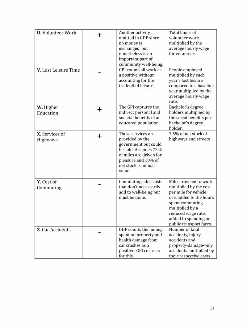
U. Volunteer Work + Another activity omitted in GDP since no money is exchanged, but nonetheless is an important part of community well-being.

Total hours of volunteer work multiplied by the average hourly wage for volunteers.

V. Lost Leisure Time - GPI counts all work as a positive without accounting for the tradeoff of leisure.

People employed multiplied by each year’s lost leisure compared to a baseline year multiplied by the average hourly wage rate.

W. Higher Education + The GPI captures the

indirect personal and societal benefits of an educated population.

Bachelor’s degree holders multiplied by the social benefits per bachelor’s degree holder.

X. Services of Highways + These services are

provided by the government but could be sold. Assumes 75% of miles are driven for pleasure and 10% of net stock is annual value.

7.5% of net stock of highways and streets

Y. Cost of Commuting - Commuting adds costs

that don’t necessarily add to well-being but must be done.

Miles traveled to work multiplied by the cost per mile for vehicle use, added to the hours spent commuting multiplied by a reduced wage rate, added to spending on public transport fares.

Z. Car Accidents - GDP counts the money spent on property and health damage from car crashes as a positive. GPI corrects for this.

Number of fatal accidents, injury accidents and property-damage-only accidents multiplied by their respective costs.

12

CHAPTER 3: ECONOMIC COMPONENTS OF THE GPI

Personal Consumption

The foundation or starting point for calculating the GPI is personal consumption spending

by households on goods and services. GDP, which displays the total monetary value of what

is produced, does not reveal what a Colorado household consumes. Since it is ultimately the

consumption of goods and services that brings about material welfare, measuring personal

consumption is the appropriate starting point for an indicator of well-being.

Personal Consumption Expenditure, as the metric is known, is not unlike GDP since

personal consumption makes up about 70 percent of GDP. Everything that households

spend their money on: groceries, clothes, childcare, healthcare, education, transportation,

recreation and entertainment, etc., is counted in personal consumption. As the starting

point, personal consumption is the baseline measure from which all other factors in the GPI

are added or subtracted.

The Bureau of Economic Analysis (BEA) does not measure personal consumption data at

the state level. It does however measure personal income. Thus, GPI studies use the national

ratio of consumption to income and state-level data on personal income to derive state-level

consumption statistics.

In Table 3 we derive personal consumption each decade as an example. Starting with

personal income (BEA) which is adjusted for inflation into 2000 dollars, we multiply by the

average U.S. ratio of consumption to income — also known as the propensity to consume —

to get personal consumption per capita for Colorado.

It should be noted that all indicators used in the Colorado GPI are in real 2000 dollar values.

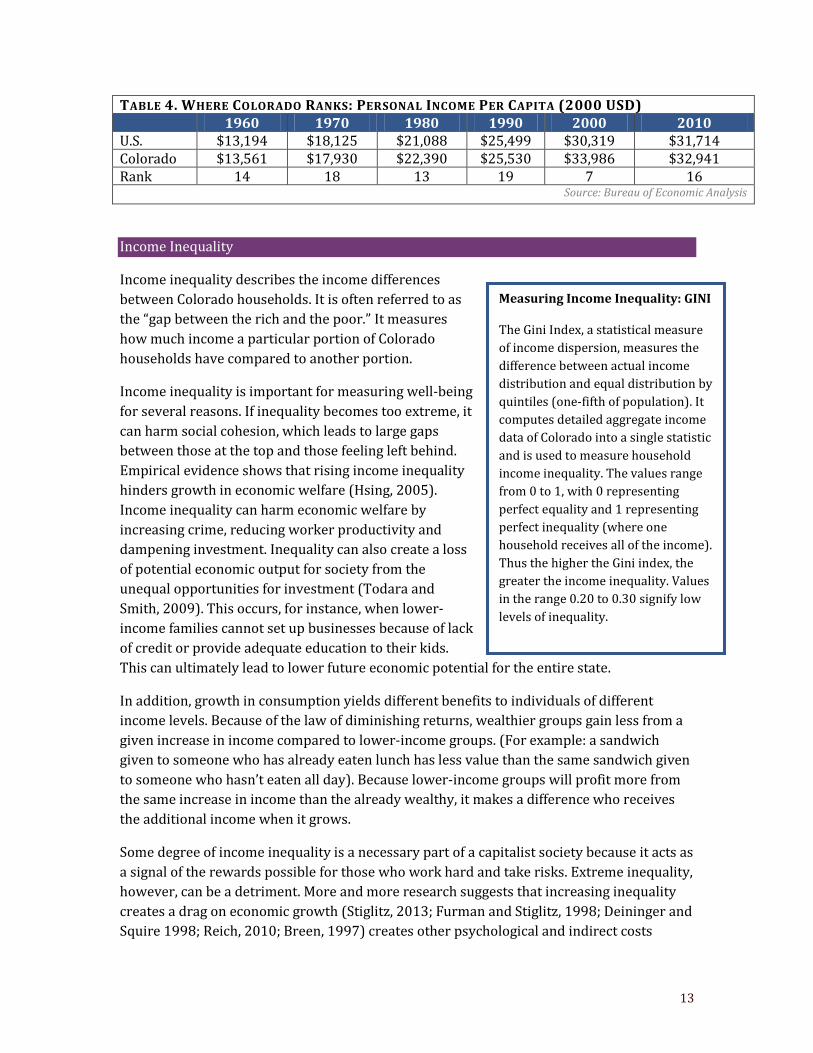
As Table 4 illustrates, consumption per capita has almost tripled since 1960. Colorado is a

fairly wealthy state — ranking 16th in personal income per capita in 2011. In recent

decades, Colorado has been among the wealthier states. Colorado was the 14th wealthiest

state in 1960.

TABLE 3. DERIVATION OF PERSONAL CONSUMPTION PER CAPITA (2000 USD) 1960 1970 1980 1990 2000 2010

Personal Income per capita Colorado

$13,562 $17,930 $22,390 $25,530 $33,986 $33,249

Ratio, Income-Consumption: U.S.

78% 75% 76% 78% 79% 82%

Personal Consumption per capita Colorado

$10,644 $13,432 $16,957 $19,914 $26,777 $27,278

Source: Bureau of Economic Analysis

13

TABLE 4. WHERE COLORADO RANKS: PERSONAL INCOME PER CAPITA (2000 USD) 1960 1970 1980 1990 2000 2010 U.S. $13,194 $18,125 $21,088 $25,499 $30,319 $31,714 Colorado $13,561 $17,930 $22,390 $25,530 $33,986 $32,941 Rank 14 18 13 19 7 16

Source: Bureau of Economic Analysis

Income Inequality

Income inequality describes the income differences

between Colorado households. It is often referred to as

the “gap between the rich and the poor.” It measures

how much income a particular portion of Colorado

households have compared to another portion.

Income inequality is important for measuring well-being

for several reasons. If inequality becomes too extreme, it

can harm social cohesion, which leads to large gaps

between those at the top and those feeling left behind.

Empirical evidence shows that rising income inequality

hinders growth in economic welfare (Hsing, 2005).

Income inequality can harm economic welfare by

increasing crime, reducing worker productivity and

dampening investment. Inequality can also create a loss

of potential economic output for society from the

unequal opportunities for investment (Todara and

Smith, 2009). This occurs, for instance, when lower-

income families cannot set up businesses because of lack

of credit or provide adequate education to their kids.

This can ultimately lead to lower future economic potential for the entire state.

In addition, growth in consumption yields different benefits to individuals of different

income levels. Because of the law of diminishing returns, wealthier groups gain less from a

given increase in income compared to lower-income groups. (For example: a sandwich

given to someone who has already eaten lunch has less value than the same sandwich given

to someone who hasn’t eaten all day). Because lower-income groups will profit more from

the same increase in income than the already wealthy, it makes a difference who receives

the additional income when it grows.

Some degree of income inequality is a necessary part of a capitalist society because it acts as

a signal of the rewards possible for those who work hard and take risks. Extreme inequality,

however, can be a detriment. More and more research suggests that increasing inequality

creates a drag on economic growth (Stiglitz, 2013; Furman and Stiglitz, 1998; Deininger and

Squire 1998; Reich, 2010; Breen, 1997) creates other psychological and indirect costs

Measuring Income Inequality: GINI

The Gini Index, a statistical measure

of income dispersion, measures the

difference between actual income

distribution and equal distribution by

quintiles (one-fifth of population). It

computes detailed aggregate income

data of Colorado into a single statistic

and is used to measure household

income inequality. The values range

from 0 to 1, with 0 representing

perfect equality and 1 representing

perfect inequality (where one

household receives all of the income).

Thus the higher the Gini index, the

greater the income inequality. Values

in the range 0.20 to 0.30 signify low

levels of inequality.

14

(Frank, 2000; Wilkinson 2010; Wisman 2011) causes increased poverty (Iceland, 2003) and

makes the economy more susceptible and more vulnerable to economic crises (Wisman,

2013; Georgopoulos et al, 2010; Holt and Greenwood 2012). Others argue that income

inequality in a given year is not such a bad thing as long as there is upward mobility in

society. If families in lower-income groups can advance to high-income groups, then

inequality isn’t necessarily terrible. This is a valid point; assessing inequality should be

considered in the context of upward societal mobility. Recent survey evidence shows that

Americans dramatically underestimate the level of income inequality and show a desire for

a more equal distribution of wealth than the status quo. (Norton and Ariely, 2011).

Income distribution is factored into the GPI from the notion that inequality directly relates

to social cohesion and economic welfare which is predicated on the assumption that

inequality represents a social cost (Anielski and Rowe, 1998). The Colorado GPI

incorporates income inequality by discounting personal consumption expenditures by the

amount of inequality in each year using an income distribution index. GPI does this by

choosing the year in which inequality was lowest and using deviations from that base year

to weight personal consumption. This method assumes that, from an economic well-being

perspective, the lowest level of income inequality is the best condition. The year 1970 was

used as the base year in previous GPI studies since it was the year in which the U.S.

experienced the lowest levels of income inequality. To maintain comparability with other

state-level GPI studies, we also indexed Colorado’s Gini coefficients with the base year 1970

set to 100, even though Colorado had its lowest level of inequality in 1962. Since Colorado

had a few years before 1970 with lower income inequality, the adjusted personal

consumption is actually higher than personal consumption in some of those years.

See Table 5 for calculations. Column C equals column A divided by column B. As inequality

grows, adjusted personal consumption shrinks — reducing well-being.

TABLE 5. ADJUSTING PERSONAL CONSUMPTION FOR INCOME INEQUALITY 1960 1970 1980 1990 2000 2010

A Personal consumption per capita Colorado

$10,644 $13,432 $16,957 $19,914 $26,777 $27,278

B Indexed GINI coefficient

95 100 108 125 131 129

C Adjusted personal consumption

$11,211 $13,432 $15,679 $15,908 $20,464 $21,214

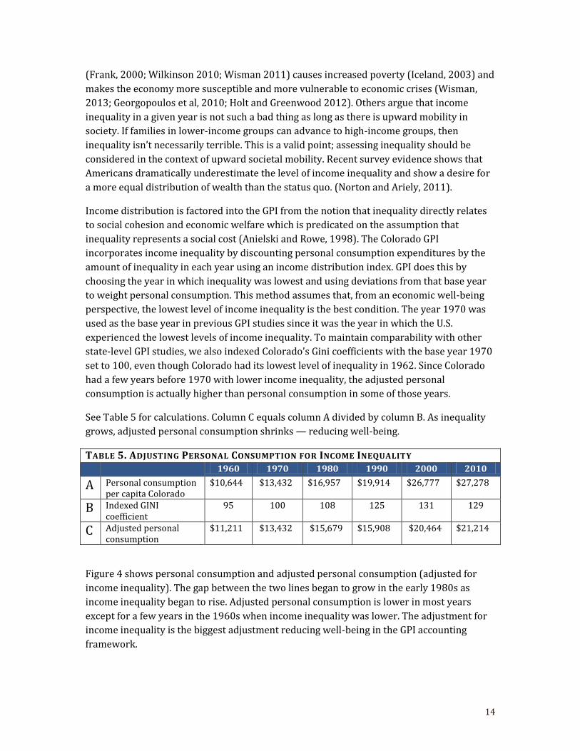
Figure 4 shows personal consumption and adjusted personal consumption (adjusted for

income inequality). The gap between the two lines began to grow in the early 1980s as

income inequality began to rise. Adjusted personal consumption is lower in most years

except for a few years in the 1960s when income inequality was lower. The adjustment for

income inequality is the biggest adjustment reducing well-being in the GPI accounting

framework.

15

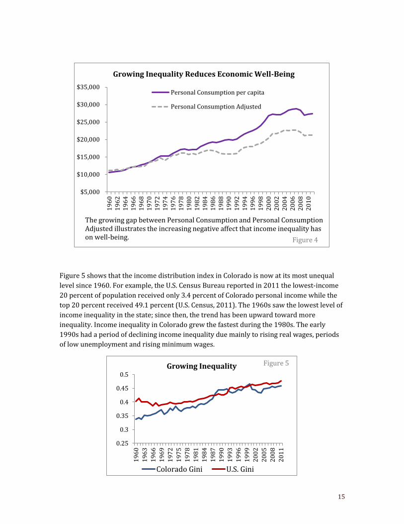
Figure 5 shows that the income distribution index in Colorado is now at its most unequal

level since 1960. For example, the U.S. Census Bureau reported in 2011 the lowest-income

20 percent of population received only 3.4 percent of Colorado personal income while the

top 20 percent received 49.1 percent (U.S. Census, 2011). The 1960s saw the lowest level of

income inequality in the state; since then, the trend has been upward toward more

inequality. Income inequality in Colorado grew the fastest during the 1980s. The early

1990s had a period of declining income inequality due mainly to rising real wages, periods

of low unemployment and rising minimum wages.

$5,000

$10,000

$15,000

$20,000

$25,000

$30,000

$35,000

19

60

19

62

19

64

19

66

19

68

19

70

19

72

19

74

19

76

19

78

19

80

19

82

19

84

19

86

19

88

19

90

19

92

19

94

19

96

19

98

20

00

20

02

20

04

20

06

20

08

20

10

Personal Consumption per capita

Personal Consumption Adjusted

Growing Inequality Reduces Economic Well-Being

The growing gap between Personal Consumption and Personal Consumption Adjusted illustrates the increasing negative affect that income inequality has on well-being. Figure 4

0.25

0.3

0.35

0.4

0.45

0.5

19

60

19

63

19

66

19

69

19

72

19

75

19

78

19

81

19

84

19

87

19

90

19

93

19

96

19

99

20

02

20

05

20

08

20

11

Growing Inequality

Colorado Gini U.S. Gini

Figure 5

16

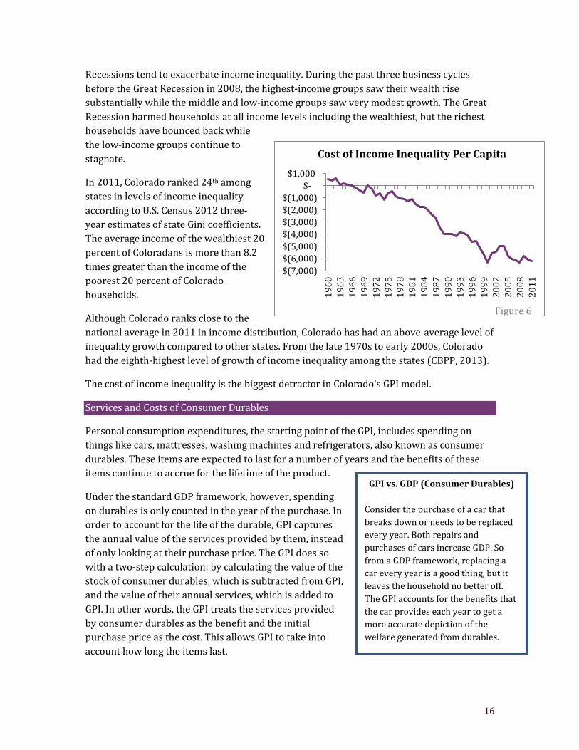
Recessions tend to exacerbate income inequality. During the past three business cycles

before the Great Recession in 2008, the highest-income groups saw their wealth rise

substantially while the middle and low-income groups saw very modest growth. The Great

Recession harmed households at all income levels including the wealthiest, but the richest

households have bounced back while

the low-income groups continue to

stagnate.

In 2011, Colorado ranked 24th among

states in levels of income inequality

according to U.S. Census 2012 three-

year estimates of state Gini coefficients.

The average income of the wealthiest 20

percent of Coloradans is more than 8.2

times greater than the income of the

poorest 20 percent of Colorado

households.

Although Colorado ranks close to the

national average in 2011 in income distribution, Colorado has had an above-average level of

inequality growth compared to other states. From the late 1970s to early 2000s, Colorado

had the eighth-highest level of growth of income inequality among the states (CBPP, 2013).

The cost of income inequality is the biggest detractor in Colorado’s GPI model.

Services and Costs of Consumer Durables

Personal consumption expenditures, the starting point of the GPI, includes spending on

things like cars, mattresses, washing machines and refrigerators, also known as consumer

durables. These items are expected to last for a number of years and the benefits of these

items continue to accrue for the lifetime of the product.

Under the standard GDP framework, however, spending

on durables is only counted in the year of the purchase. In

order to account for the life of the durable, GPI captures

the annual value of the services provided by them, instead

of only looking at their purchase price. The GPI does so

with a two-step calculation: by calculating the value of the

stock of consumer durables, which is subtracted from GPI,

and the value of their annual services, which is added to

GPI. In other words, the GPI treats the services provided

by consumer durables as the benefit and the initial

purchase price as the cost. This allows GPI to take into

account how long the items last.

GPI vs. GDP (Consumer Durables)

Consider the purchase of a car that

breaks down or needs to be replaced

every year. Both repairs and

purchases of cars increase GDP. So

from a GDP framework, replacing a

car every year is a good thing, but it

leaves the household no better off.

The GPI accounts for the benefits that

the car provides each year to get a

more accurate depiction of the

welfare generated from durables.

$(7,000)

$(6,000)

$(5,000)

$(4,000)

$(3,000)

$(2,000)

$(1,000)

$-

$1,000

19

60

19

63

19

66

19

69

19

72

19

75

19

78

19

81

19

84

19

87

19

90

19

93

19

96

19

99

20

02

20

05

20

08

20

11

Cost of Income Inequality Per Capita

Figure 6

17

The costs of consumer durables are calculated from national estimates of the cost of

consumer durables and are scaled-down for Colorado based on the ratio of state personal

income to the national total. Economic theory defines the annual services derived from

durables as the sum of the depreciation rate and interest rate (Talberth, 2007). The interest

rate is included under the assumption that the purchaser of the durable could have received

that much interest from investing that money used to purchase the durable. Based on the

assumption that durables last on average eight years, which translates into a 12.5 percent

depreciation rate and a 7.5 percent interest rate, the annual value of services from durables

is estimated as 20 percent of the

total stock of durables in

Colorado.

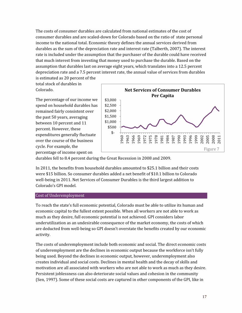
The percentage of our income we

spend on household durables has

remained fairly consistent over

the past 50 years, averaging

between 10 percent and 11

percent. However, these

expenditures generally fluctuate

over the course of the business

cycle. For example, the

percentage of income spent on

durables fell to 8.4 percent during the Great Recession in 2008 and 2009.

In 2011, the benefits from household durables amounted to $25.1 billion and their costs

were $15 billion. So consumer durables added a net benefit of $10.1 billion to Colorado

well-being in 2011. Net Services of Consumer Durables is the third largest addition to

Colorado’s GPI model.

Cost of Underemployment

To reach the state’s full economic potential, Colorado must be able to utilize its human and

economic capital to the fullest extent possible. When all workers are not able to work as

much as they desire, full economic potential is not achieved. GPI considers labor

underutilization as an undesirable consequence of the market economy, the costs of which

are deducted from well-being so GPI doesn’t overstate the benefits created by our economic

activity.

The costs of underemployment include both economic and social. The direct economic costs

of underemployment are the declines in economic output because the workforce isn’t fully

being used. Beyond the declines in economic output, however, underemployment also

creates individual and social costs. Declines in mental health and the decay of skills and

motivation are all associated with workers who are not able to work as much as they desire.

Persistent joblessness can also deteriorate social values and cohesion in the community

(Sen, 1997). Some of these social costs are captured in other components of the GPI, like in

$-

$500

$1,000

$1,500

$2,000

$2,500

$3,000

19

60

19

63

19

66

19

69

19

72

19

75

19

78

19

81

19

84

19

87

19

90

19

93

19

96

19

99

20

02

20

05

20

08

20

11

Net Services of Consumer Durables Per Capita

Figure 7

18

the divorce indicator or crime indicator, but because not all of the social costs of

underemployment are accounted for, GPI subtracts the cost of underemployment from

economic well-being. GPI does so by treating each hour of underemployment as a cost.

(Even though GPI places value on free time, which is captured in the lost leisure indicator, it

recognizes that forced free time, i.e., hours that the individual would rather spend working

but cannot, are a social burden.)

Underemployment is a broader category than unemployment. It refers to persons who are

chronically unemployed, who have given up on looking for work, who would prefer to work

full-time but are unable or who are constrained by barriers like child care or transportation.

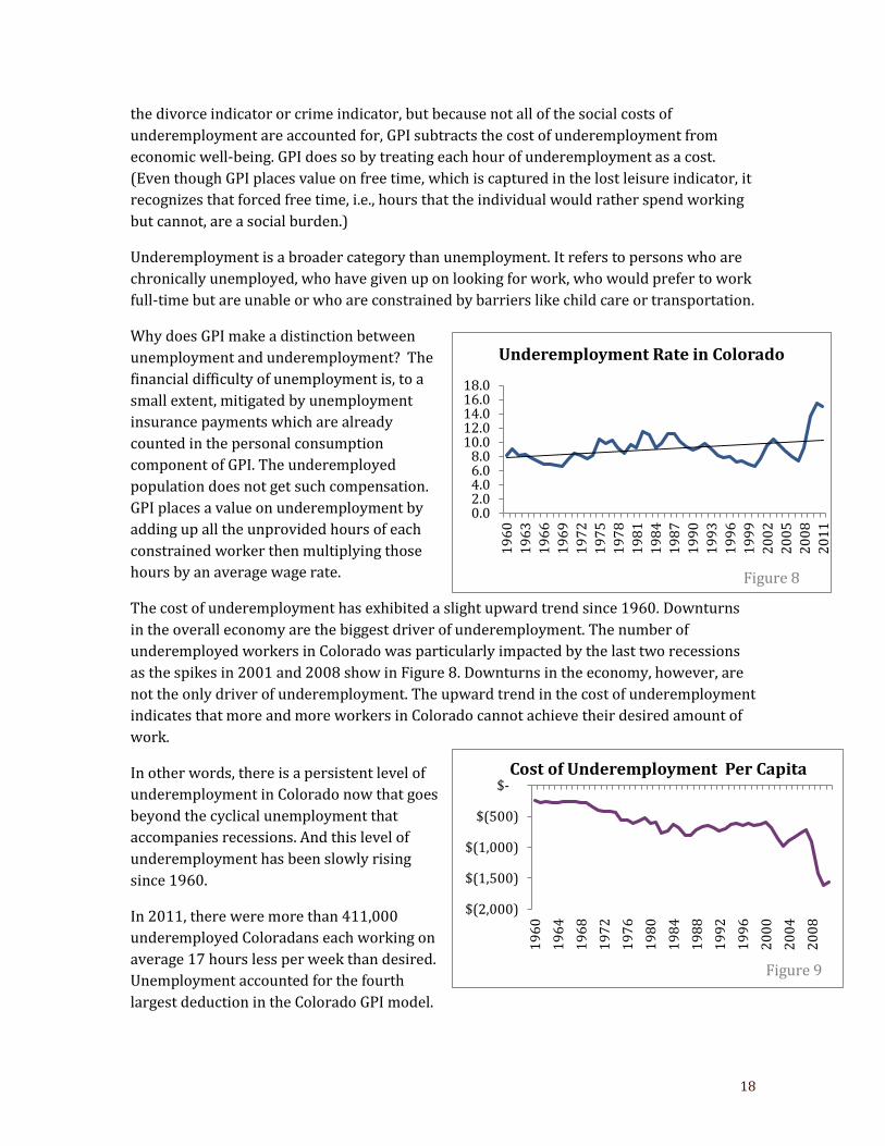
Why does GPI make a distinction between

unemployment and underemployment? The

financial difficulty of unemployment is, to a

small extent, mitigated by unemployment

insurance payments which are already

counted in the personal consumption

component of GPI. The underemployed

population does not get such compensation.

GPI places a value on underemployment by

adding up all the unprovided hours of each

constrained worker then multiplying those

hours by an average wage rate.

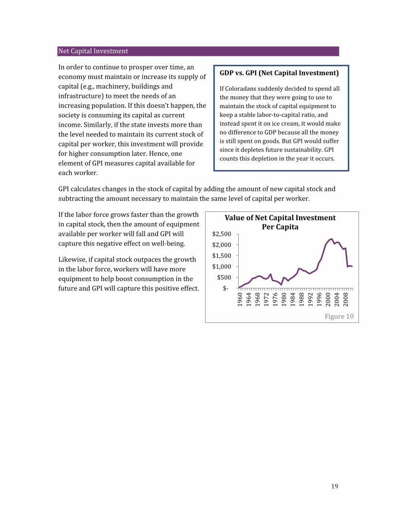
The cost of underemployment has exhibited a slight upward trend since 1960. Downturns

in the overall economy are the biggest driver of underemployment. The number of

underemployed workers in Colorado was particularly impacted by the last two recessions

as the spikes in 2001 and 2008 show in Figure 8. Downturns in the economy, however, are

not the only driver of underemployment. The upward trend in the cost of underemployment

indicates that more and more workers in Colorado cannot achieve their desired amount of

work.

In other words, there is a persistent level of

underemployment in Colorado now that goes

beyond the cyclical unemployment that

accompanies recessions. And this level of

underemployment has been slowly rising

since 1960.

In 2011, there were more than 411,000

underemployed Coloradans each working on

average 17 hours less per week than desired.

Unemployment accounted for the fourth

largest deduction in the Colorado GPI model.

$(2,000)

$(1,500)

$(1,000)

$(500)

$-

19

60

19

64

19

68

19

72

19

76

19

80

19

84

19

88

19

92

19

96

20

00

20

04

20

08

Cost of Underemployment Per Capita

Figure 9

0.02.04.06.08.0

10.012.014.016.018.0

19

60

19

63

19

66

19

69

19

72

19

75

19

78

19

81

19

84

19

87

19

90

19

93

19

96

19

99

20

02

20

05

20

08

20

11

Underemployment Rate in Colorado

Figure 8

19

Net Capital Investment

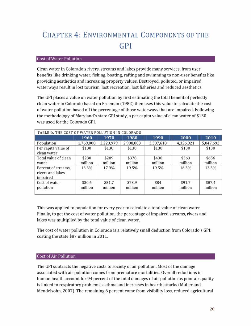
In order to continue to prosper over time, an

economy must maintain or increase its supply of

capital (e.g., machinery, buildings and

infrastructure) to meet the needs of an

increasing population. If this doesn’t happen, the

society is consuming its capital as current

income. Similarly, if the state invests more than

the level needed to maintain its current stock of

capital per worker, this investment will provide

for higher consumption later. Hence, one

element of GPI measures capital available for

each worker.

GPI calculates changes in the stock of capital by adding the amount of new capital stock and

subtracting the amount necessary to maintain the same level of capital per worker.

If the labor force grows faster than the growth

in capital stock, then the amount of equipment

available per worker will fall and GPI will

capture this negative effect on well-being.

Likewise, if capital stock outpaces the growth

in the labor force, workers will have more

equipment to help boost consumption in the

future and GPI will capture this positive effect.

GDP vs. GPI (Net Capital Investment)

If Coloradans suddenly decided to spend all

the money that they were going to use to

maintain the stock of capital equipment to

keep a stable labor-to-capital ratio, and

instead spent it on ice cream, it would make

no difference to GDP because all the money

is still spent on goods. But GPI would suffer

since it depletes future sustainability. GPI

counts this depletion in the year it occurs.

$-

$500

$1,000

$1,500

$2,000

$2,5001

96

0

19

64

19

68

19

72

19

76

19

80

19

84

19

88

19

92

19

96

20

00

20

04

20

08

Value of Net Capital Investment Per Capita

Figure 10

20

CHAPTER 4: ENVIRONMENTAL COMPONENTS OF THE

GPI Cost of Water Pollution

Clean water in Colorado’s rivers, streams and lakes provide many services, from user

benefits like drinking water, fishing, boating, rafting and swimming to non-user benefits like

providing aesthetics and increasing property values. Destroyed, polluted, or impaired

waterways result in lost tourism, lost recreation, lost fisheries and reduced aesthetics.

The GPI places a value on water pollution by first estimating the total benefit of perfectly

clean water in Colorado based on Freeman (1982) then uses this value to calculate the cost

of water pollution based off the percentage of those waterways that are impaired. Following

the methodology of Maryland’s state GPI study, a per capita value of clean water of $130

was used for the Colorado GPI.

TABLE 6. THE COST OF WATER POLLUTION IN COLORADO 1960 1970 1980 1990 2000 2010 Population 1,769,000 2,223,979 2,908,803 3,307,618 4,326,921 5,047,692 Per capita value of clean water

$130 $130 $130 $130 $130 $130

Total value of clean water

$230 million

$289 million

$378 million

$430 million

$563 million

$656 million

Percent of streams, rivers and lakes impaired

13.3% 17.9% 19.5% 19.5% 16.3% 13.3%

Cost of water pollution

$30.6 million

$51.7 million

$73.9 million

$84 million

$91.7 million

$87.4 million

This was applied to population for every year to calculate a total value of clean water.

Finally, to get the cost of water pollution, the percentage of impaired streams, rivers and

lakes was multiplied by the total value of clean water.

The cost of water pollution in Colorado is a relatively small deduction from Colorado’s GPI:

costing the state $87 million in 2011.

Cost of Air Pollution

The GPI subtracts the negative costs to society of air pollution. Most of the damage

associated with air pollution comes from premature mortalities. Overall reductions in

human health account for 94 percent of the total damages of air pollution as poor air quality

is linked to respiratory problems, asthma and increases in hearth attacks (Muller and

Mendelsohn, 2007). The remaining 6 percent come from visibility loss, reduced agricultural

21

yield, reduced timber yield, accelerated depreciation of man-made material and impaired

forest health.

Five pollutants were included in the analysis. Two were “particulate matter,” also known as

particle pollution: large particulate matter (PM10) and fine particulate matter (PM2.5),

which is a mixture of small particles and liquid droplets. The EPA is concerned with

particles less than 10 micrometers in diameter because those particles can easily enter the

lungs through the nose and throat.

The third pollutant was Nitrogen Oxides (NOx) which are commonly caused by vehicle

emissions. The fourth was Sulfur Oxides (SOx), which are mainly generated from industrial

processes, and fifth was Volatile Organic Compounds (VOCs), which are emitted gases from

a wide range of products from paints to glues to markers.

The Environmental Protection Agency’s National Emissions Inventory Database has been

tracking state level pollution emissions since 1990 and national level emissions since 1975.

For prior year figures, Aneilski and Rowe’s (1999) assumptions were used: air quality

declined 2.4 percent per year in the 1960s.

GPI estimates the cost of pollution by multiplying the emissions estimates for each of the

five pollutants by the per-ton cost for each reported by Muller and Mendelsohn (2007). The

per ton damages in Colorado in 2000 dollars of large particulate matter is $544 per ton, fine

particulate matter damages were $3,462 per ton. The per ton damages of Nitrogen Oxides

were $273 per ton. Sulfur Oxide damages were $1,261 per ton and those from Volatile

Organic Compounds were $676 per ton.

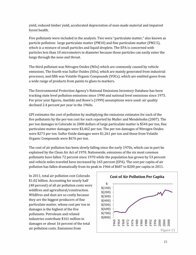
The cost of air pollution has been slowly falling since the early 1970s, which can in part be

explained by the Clean Air Act of 1970. Nationwide, emissions of the six most common

pollutants have fallen 72 percent since 1970 while the population has grown by 53 percent

and vehicle miles traveled have increased by 165 percent (EPA). The cost per capita of air

pollution has fallen dramatically from its peak in 1966 of $687 to $200 per capita in 2011.

In 2011, total air pollution cost Colorado

$1.02 billion. Accounting for nearly half

(48 percent) of all air pollution costs were

wildfires and agricultural/construction.

Wildfires and dust are so costly because

they are the biggest producers of fine

particulate matter, whose cost per ton in

damages is the highest of the five

pollutants. Petroleum and related

industries contribute $161 million in

damages or about 16 percent of the total

air pollution costs. Emissions from

$(800)

$(700)

$(600)

$(500)

$(400)

$(300)

$(200)

$(100)

$-

19

60

19

64

19

68

19

72

19

76

19

80

19

84

19

88

19

92

19

96

20

00

20

04

20

08

Cost of Air Pollution Per Capita

Figure 11

22

automobiles cost Colorado $70 million and accounted for 7 percent of the total pollution

cost. Automobiles account for a third of all nitrogen oxide emissions in the state.

Due to the state’s climate and topography, pollution emissions disporportionately impact

Coloradans because of a condition called “temperature inversion,” which occurs when warm

air traps cold air near Colorado’s land surface. This condition affects large mountain valleys

the most (Doesken, 2007). When temperature inversions occur, a regularity in the winter,

air pollution can’t escape into the atmosphere. The warm layer of air acts as a cap, trapping

pollution near ground level.

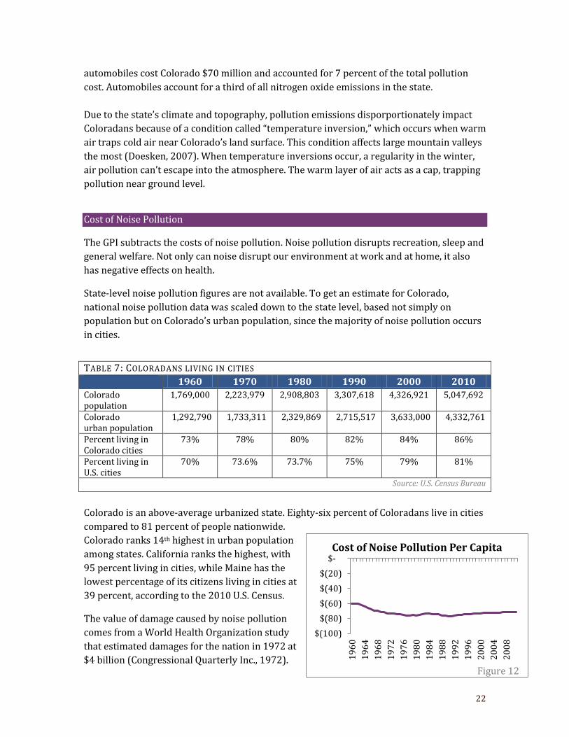
Cost of Noise Pollution

The GPI subtracts the costs of noise pollution. Noise pollution disrupts recreation, sleep and

general welfare. Not only can noise disrupt our environment at work and at home, it also

has negative effects on health.

State-level noise pollution figures are not available. To get an estimate for Colorado,

national noise pollution data was scaled down to the state level, based not simply on

population but on Colorado’s urban population, since the majority of noise pollution occurs

in cities.

Colorado is an above-average urbanized state. Eighty-six percent of Coloradans live in cities

compared to 81 percent of people nationwide.

Colorado ranks 14th highest in urban population

among states. California ranks the highest, with

95 percent living in cities, while Maine has the

lowest percentage of its citizens living in cities at

39 percent, according to the 2010 U.S. Census.

The value of damage caused by noise pollution

comes from a World Health Organization study

that estimated damages for the nation in 1972 at

$4 billion (Congressional Quarterly Inc., 1972).

TABLE 7: COLORADANS LIVING IN CITIES

1960 1970 1980 1990 2000 2010 Colorado population

1,769,000 2,223,979 2,908,803 3,307,618 4,326,921 5,047,692

Colorado urban population

1,292,790 1,733,311 2,329,869 2,715,517 3,633,000 4,332,761

Percent living in Colorado cities

73% 78% 80% 82% 84% 86%

Percent living in U.S. cities

70% 73.6% 73.7% 75% 79% 81%

Source: U.S. Census Bureau

$(100)

$(80)

$(60)

$(40)

$(20)

$-

19

60

19

64

19

68

19

72

19

76

19

80

19

84

19

88

19

92

19

96

20

00

20

04

20

08

Cost of Noise Pollution Per Capita

Figure 12

23

This estimate used by Talberth (2007) amounts to $14.6 billion in 2000 dollars.

The average cost of noise pollution per person living in an urban area was $83 in 2011. In

Colorado, the total cost of noise pollution has steadily increased due to the state’s increased

urbanization. In 2011, noise pollution cost Colorado $363 million, a very moderate

reduction in well-being.

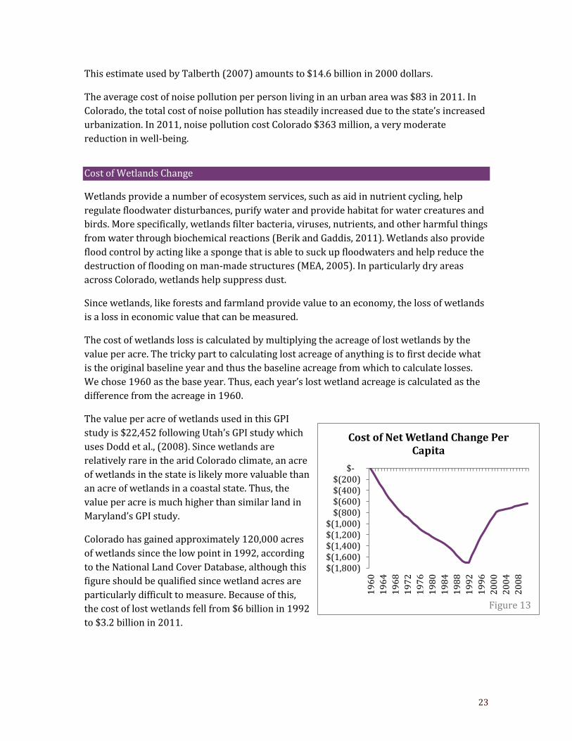
Cost of Wetlands Change

Wetlands provide a number of ecosystem services, such as aid in nutrient cycling, help

regulate floodwater disturbances, purify water and provide habitat for water creatures and

birds. More specifically, wetlands filter bacteria, viruses, nutrients, and other harmful things

from water through biochemical reactions (Berik and Gaddis, 2011). Wetlands also provide

flood control by acting like a sponge that is able to suck up floodwaters and help reduce the

destruction of flooding on man-made structures (MEA, 2005). In particularly dry areas

across Colorado, wetlands help suppress dust.

Since wetlands, like forests and farmland provide value to an economy, the loss of wetlands

is a loss in economic value that can be measured.

The cost of wetlands loss is calculated by multiplying the acreage of lost wetlands by the

value per acre. The tricky part to calculating lost acreage of anything is to first decide what

is the original baseline year and thus the baseline acreage from which to calculate losses.

We chose 1960 as the base year. Thus, each year’s lost wetland acreage is calculated as the

difference from the acreage in 1960.

The value per acre of wetlands used in this GPI

study is $22,452 following Utah’s GPI study which

uses Dodd et al., (2008). Since wetlands are

relatively rare in the arid Colorado climate, an acre

of wetlands in the state is likely more valuable than

an acre of wetlands in a coastal state. Thus, the

value per acre is much higher than similar land in

Maryland’s GPI study.

Colorado has gained approximately 120,000 acres

of wetlands since the low point in 1992, according

to the National Land Cover Database, although this

figure should be qualified since wetland acres are

particularly difficult to measure. Because of this,

the cost of lost wetlands fell from $6 billion in 1992

to $3.2 billion in 2011.

$(1,800) $(1,600) $(1,400) $(1,200) $(1,000)

$(800) $(600) $(400) $(200)

$-

19

60

19

64

19

68

19

72

19

76

19

80

19

84

19

88

19

92

19

96

20

00

20

04

20

08

Cost of Net Wetland Change Per Capita

Figure 13

24

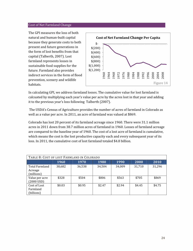
Cost of Net Farmland Change

The GPI measures the loss of both

natural and human-built capital

because they generate costs to both

present and future generations in

the form of lost benefits from that

capital (Talberth, 2007). Lost

farmland represents losses in

sustainable food supplies for the

future. Farmland also provides

indirect services in the form of flood

prevention, scenery and wildlife

habitats.

In calculating GPI, we address farmland losses. The cumulative value for lost farmland is

calcuated by multiplying each year’s value per acre by the acres lost in that year and adding

it to the previous year’s loss following Talberth (2007).

The USDA’s Census of Agriculture provides the number of acres of farmland in Colorado as

well as a value per acre. In 2011, an acre of farmland was valued at $869.

Colorado has lost 20 percent of its farmland acreage since 1960. There were 31.1 million

acres in 2011 down from 38.7 million acres of farmland in 1960. Losses of farmland acreage

are compared to the baseline year of 1960. The cost of a lost acre of farmland is cumulative,

which means the cost is the lost productive capacity each and every subsequent year of its

loss. In 2011, the cumulative cost of lost farmland totaled $4.8 billion.

TABLE 8: COST OF LOST FARMLAND IN COLORADO

1960 1970 1980 1990 2000 2010 Total Farmland Acreage (millions)

38,682 36,538 34,504 34,009 31,710 31,296

Value per acre (2000 USD)

$328 $504 $806 $563 $705 $869

Cost of Lost Farmland (billions)

$0.03 $0.95 $2.47 $2.94 $4.45 $4.75

$(1,200)

$(1,000)

$(800)

$(600)

$(400)

$(200)

$-

19

60

19

64

19

68

19

72

19

76

19

80

19

84

19

88

19

92

19

96

20

00

20

04

20

08

Cost of Net Farmland Change Per Capita

Figure 14

25

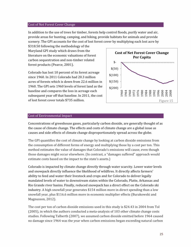
Cost of Net Forest Cover Change

In addition to the use of trees for timber, forests help control floods, purify water and air,

provide areas for hunting, camping, and hiking, provide habitats for animals and provide

scenery. The GPI accounts for the cost of lost forest cover by multiplying each lost acre by

$318.50 following the methodology of the

Maryland GPI study which draws from the

literature on the economic valuations of forest

carbon sequestration and non-timber related

forest products (Pearce, 2001).

Colorado has lost 10 percent of its forest acreage

since 1960. In 2011 Colorado had 20.3 million

acres of forests which is down from 22.6 million in

1960. The GPI sets 1960 levels of forest land as the

baseline and compares the loss in acreage each

subsequent year off that baseline. In 2011, the cost

of lost forest cover totals $735 million.

Cost of Environmental Impact

Concentrations of greenhouse gases, particularly carbon dioxide, are generally thought of as

the cause of climate change. The effects and costs of climate change are a global issue as

causes and side effects of climate change disproportionately spread across the globe.

The GPI quantifies the cost of climate change by looking at carbon dioxide emissions from

the consumption of different forms of energy and multiplying those by a cost per ton. This

method estimates the value of damages that Colorado’s emissions will cause, even though

those damages might occur elsewhere. (In contrast, a “damages suffered” approach would

estimate costs based on the impact to the state’s assets.)

Colorado is impacted by climate change directly through water scarcity. Lower water levels

and snowpack directly influence the likelihood of wildfires. It directly affects farmers’

ability to feed and water their livestock and crops and for Colorado to deliver legally

mandated levels of water to downstream states within the Colorado, Platte, Arkansas and

Rio Grande river basins. Finally, reduced snowpack has a direct effect on the Colorado ski

industry. A high snowfall year generates $154 million more in direct spending than a low

snowfall year, plus $116.6 million more in economic multiplier effects (Burakowski and

Magnusson, 2012).

The cost per ton of carbon dioxide emissions used in this study is $24.43 in 2004 from Tol

(2005), in which the authors conducted a meta-analysis of 103 other climate change costs

studies. Following Talberth (2007), we assumed carbon dioxide emitted before 1964 caused

no damage since 1964 was the year when carbon emissions began exceeding natural carbon

$(200)

$(150)

$(100)

$(50)

$-

19

60

19

64

19

68

19

72

19

76

19

80

19

84

19

88

19

92

19

96

20

00

20

04

20

08

Cost of Net Forest Cover Change Per Capita

Figure 15

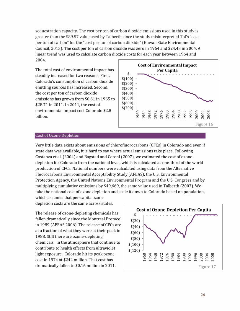
26

sequestration capacity. The cost per ton of carbon dioxide emissions used in this study is

greater than the $89.57 value used by Talberth since the study misinterpreted Tol’s “cost

per ton of carbon” for the “cost per ton of carbon dioxide” (Hawaii State Environmental

Council, 2013). The cost per ton of carbon dioxide was zero in 1964 and $24.43 in 2004. A

linear trend was used to calculate carbon dioxide costs for each year between 1964 and

2004.

The total cost of environmental impact has

steadily increased for two reasons. First,

Colorado’s consumption of carbon dioxide

emitting sources has increased. Second,

the cost per ton of carbon dioxide

emissions has grown from $0.61 in 1965 to

$28.71 in 2011. In 2011, the cost of

environmental impact cost Colorado $2.8

billion.

Cost of Ozone Depletion

Very little data exists about emissions of chlorofluorocarbons (CFCs) in Colorado and even if

state data was available, it is hard to say where actual emissions take place. Following

Costanza et al. (2004) and Bagstad and Ceroni (2007), we estimated the cost of ozone

depletion for Colorado from the national level, which is calculated as one-third of the world

production of CFCs. National numbers were calculated using data from the Alternative

Fluorocarbons Environmental Acceptability Study (AFEAS), the U.S. Environmental

Protection Agency, the United Nations Environmental Program and the U.S. Congress and by

multiplying cumulative emissions by $49,669, the same value used in Talberth (2007). We

take the national cost of ozone depletion and scale it down to Colorado based on population,

which assumes that per-capita ozone

depletion costs are the same across states.

The release of ozone-depleting chemicals has

fallen dramatically since the Montreal Protocol

in 1989 (AFEAS 2006). The release of CFCs are

at a fraction of what they were at their peak in

1988. Still there are ozone-depleting

chemicals in the atmosphere that continue to

contribute to health effects from ultraviolet

light exposure. Colorado hit its peak ozone

cost in 1974 at $242 million. That cost has

dramatically fallen to $0.16 million in 2011.

$(700) $(600) $(500) $(400) $(300) $(200) $(100)

$-

19

60

19

64

19

68

19

72

19

76

19

80

19

84

19

88

19

92

19

96

20

00

20

04

20

08

Cost of Environmental Impact Per Capita

Figure 16

$(120)

$(100)

$(80)

$(60)

$(40)

$(20)

$-

19

60

19

64

19

68

19

72

19

76

19

80

19

84

19

88

19

92

19

96

20

00

20

04

20

08

Cost of Ozone Depletion Per Capita

Figure 17

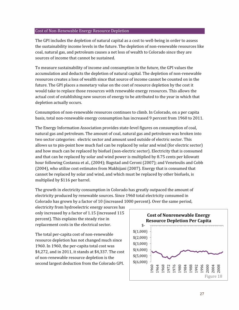
27

Cost of Non-Renewable Energy Resource Depletion

The GPI includes the depletion of natural capital as a cost to well-being in order to assess

the sustainability income levels in the future. The depletion of non-renewable resources like

coal, natural gas, and petroleum causes a net loss of wealth to Colorado since they are

sources of income that cannot be sustained.

To measure sustainability of income and consumption in the future, the GPI values the

accumulation and deducts the depletion of natural capital. The depletion of non-renewable

resources creates a loss of wealth since that source of income cannot be counted on in the

future. The GPI places a monetary value on the cost of resource depletion by the cost it

would take to replace those resources with renewable energy resources. This allows the

actual cost of establishing new sources of energy to be attributed to the year in which that

depletion actually occurs.

Consumption of non-renewable resources continues to climb. In Colorado, on a per capita

basis, total non-renewable energy consumption has increased 9 percent from 1960 to 2011.

The Energy Information Association provides state-level figures on consumption of coal,

natural gas and petroleum. The amount of coal, natural gas and petroleum was broken into

two sector categories: electric sector and amount used outside of electric sector. This

allows us to pin-point how much fuel can be replaced by solar and wind (for electric sector)

and how much can be replaced by biofuel (non-electric sector). Electricity that is consumed

and that can be replaced by solar and wind power is multiplied by 8.75 cents per kilowatt

hour following Costanza et al., (2004); Bagstad and Ceroni (2007); and Venetoulis and Cobb

(2004), who utilize cost estimates from Makhijani (2007). Energy that is consumed that

cannot be replaced by solar and wind, and which must be replaced by other biofuels, is

multiplied by $116 per barrel.

The growth in electricity consumption in Colorado has greatly outpaced the amount of

electricity produced by renewable sources. Since 1960 total electricity consumed in

Colorado has grown by a factor of 10 (increased 1000 percent). Over the same period,

electricity from hydroelectric energy sources has

only increased by a factor of 1.15 (increased 115

percent). This explains the steady rise in

replacement costs in the electrical sector.

The total per-capita cost of non-renewable

resource depletion has not changed much since

1960. In 1960, the per-capita total cost was

$4,272, and in 2011, it stands at $4,337. The cost

of non-renewable resource depletion is the

second largest deduction from the Colorado GPI. $(6,000)

$(5,000)

$(4,000)

$(3,000)

$(2,000)

$(1,000)

$-

19

60

19

64

19

68

19

72

19

76

19

80

19

84

19

88

19

92

19

96

20

00

20

04

20

08

Cost of Nonrenewable Energy Resource Depletion Per Capita

Figure 18

28

CHAPTER 5: SOCIAL COMPONENTS OF THE GPI

Value of Household Work

Parenting, household chores, eldercare and house maintenance are all important factors

that contribute to Coloradans’ well-being, yet they are almost entirely omitted in the

standard GDP framework. GDP does not count the value of a parent staying at home to

watch children, but paying for childcare is part of the “service sector” and adds to GDP.

Recent evidence from the American Time Use Survey shows that parents find caring for

their children to be much more exhausting than the work they do for pay, but that those

parents also find much more meaning in the time they spend with their children than at

work (Wang, 2013).

The GPI values the unpaid household work hours at the cost they could be provided if you

paid someone to do them and thus would be included in GDP. So all the hours spent doing

household work are multiplied by the hourly wage rate of what housekeepers earn in

Colorado. The average housekeeper’s wage in Colorado was $10.31 in 2011.

Hours spent doing household labor have significantly declined since 1960, falling from

1,698 hours a year per person to 832 in 2011. This means more household work is exported

to the market sector and already

counted in GDP. This distorts GDP

upward compared to earlier years,

when more household work was done

outside the market for no pay.

Overall, the value of household labor

contributed $27 billion to Colorado’s

GPI in 2011, making it the biggest

positive component of GPI. However,

the value of housework has declined

from its 1986 peak.

Cost of Family Changes

Arguably the most important asset and “service” in

America is the family (Anielski and Rowe, 1999).

Yet none of the value of families is counted in

economic terms, while at the same time, more and

more functions of the traditional family are being

displaced by the market economy such as hired

babysitters, the “television babysitter,” shopping

malls and take-out food (all of which are counted

in GDP). So, more and more household services are

being exported to the market economy. GDP treats

GDP vs. GPI (Cost of Family Changes)

In the GDP framework, divorce is counted as a positive in the form of spending to set up separate households, and to pay lawyers’ and counseling fees. The GPI methodology, however, treats divorces and family separations as having costs, because they reduce the well‐being of the individuals and children involved.

$-

$2,000

$4,000

$6,000

$8,000

$10,000

19

60

19

64

19

68

19

72

19

76

19

80

19

84

19

88

19

92

19

96

20

00

20

04

20

08

Value of Housework Per Capita

Figure 19

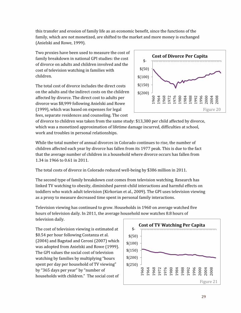
29

this transfer and erosion of family life as an economic benefit, since the functions of the

family, which are not monetized, are shifted to the market and more money is exchanged

(Anielski and Rowe, 1999).

Two proxies have been used to measure the cost of

family breakdown in national GPI studies: the cost

of divorce on adults and children involved and the

cost of television watching in families with

children.

The total cost of divorce includes the direct costs

on the adults and the indirect costs on the children

affected by divorce. The direct cost to adults per

divorce was $8,999 following Anielski and Rowe

(1999), which was based on expenses for legal

fees, separate residences and counseling. The cost

of divorce to children was taken from the same study: $13,380 per child affected by divorce,

which was a monetized approximation of lifetime damage incurred, difficulties at school,

work and troubles in personal relationships.

While the total number of annual divorces in Colorado continues to rise, the number of

children affected each year by divorce has fallen from its 1977 peak. This is due to the fact

that the average number of children in a household where divorce occurs has fallen from

1.34 in 1966 to 0.61 in 2011.

The total costs of divorce in Colorado reduced well-being by $386 million in 2011.

The second type of family breakdown cost comes from television watching. Research has

linked TV watching to obesity, diminished parent-child interactions and harmful effects on

toddlers who watch adult television (Kirkorian et al., 2009). The GPI uses television viewing

as a proxy to measure decreased time spent in personal family interactions.

Television viewing has continued to grow. Households in 1960 on average watched five

hours of television daily. In 2011, the average household now watches 8.8 hours of

television daily.

The cost of television viewing is estimated at

$0.54 per hour following Costanza et al.

(2004) and Bagstad and Ceroni (2007) which

was adopted from Anielski and Rowe (1999).

The GPI values the social cost of television

watching by families by multiplying “hours

spent per day per household of TV viewing”

by “365 days per year” by “number of

households with children.” The social cost of

$(200)

$(150)

$(100)

$(50)

$-

19

60

19

64

19

68

19

72

19

76

19

80

19

84

19

88

19

92

19

96

20

00

20

04

20

08

Cost of Divorce Per Capita

Figure 20

$(250)

$(200)

$(150)

$(100)

$(50)

$-

19

60

19

64

19

68

19

72

19

76

19

80

19

84

19

88

19

92

19

96

20

00

20

04

20

08

Cost of TV Watching Per Capita

Figure 21

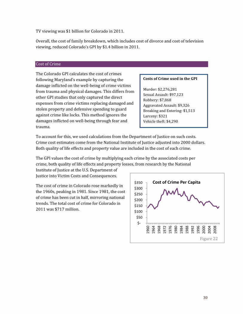
30

TV viewing was $1 billion for Colorado in 2011.

Overall, the cost of family breakdown, which includes cost of divorce and cost of television

viewing, reduced Colorado’s GPI by $1.4 billion in 2011.

Cost of Crime

The Colorado GPI calculates the cost of crimes

following Maryland’s example by capturing the

damage inflicted on the well-being of crime victims

from trauma and physical damages. This differs from

other GPI studies that only captured the direct

expenses from crime victims replacing damaged and

stolen property and defensive spending to guard

against crime like locks. This method ignores the

damages inflicted on well-being through fear and

trauma.

To account for this, we used calculations from the Department of Justice on such costs.

Crime cost estimates come from the National Institute of Justice adjusted into 2000 dollars.

Both quality of life effects and property value are included in the cost of each crime.

The GPI values the cost of crime by multiplying each crime by the associated costs per

crime, both quality of life effects and property losses, from research by the National

Institute of Justice at the U.S. Department of

Justice into Victim Costs and Consequences.

The cost of crime in Colorado rose markedly in

the 1960s, peaking in 1981. Since 1981, the cost

of crime has been cut in half, mirroring national

trends. The total cost of crime for Colorado in

2011 was $717 million.

Costs of Crime used in the GPI

Murder: $2,276,281

Sexual Assault: $97,123

Robbery: $7,868

Aggravated Assault: $9,326

Breaking and Entering: $1,513

Larceny: $321

Vehicle theft: $4,290

$-

$50

$100

$150

$200

$250

$300

$350

19

60

19

64

19

68

19

72

19

76

19

80

19

84

19

88

19

92

19

96

20

00

20

04

20

08

Cost of Crime Per Capita

Figure 22

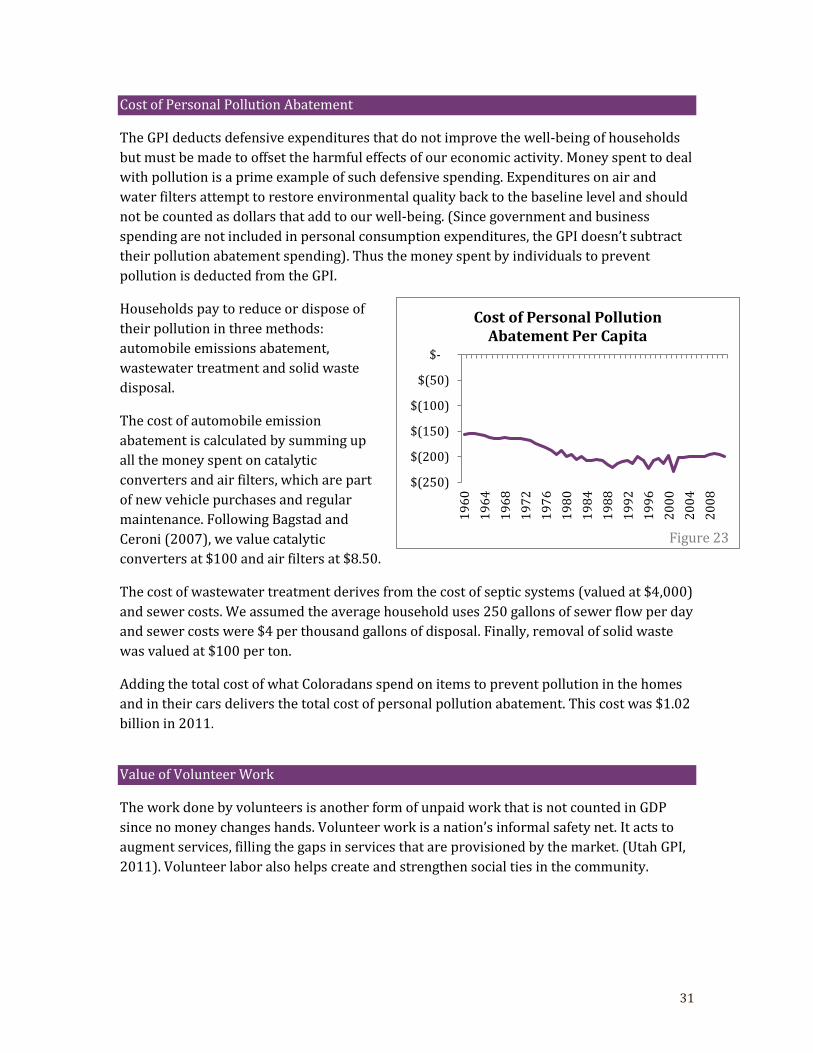
31

Cost of Personal Pollution Abatement

The GPI deducts defensive expenditures that do not improve the well-being of households

but must be made to offset the harmful effects of our economic activity. Money spent to deal

with pollution is a prime example of such defensive spending. Expenditures on air and

water filters attempt to restore environmental quality back to the baseline level and should

not be counted as dollars that add to our well-being. (Since government and business

spending are not included in personal consumption expenditures, the GPI doesn’t subtract

their pollution abatement spending). Thus the money spent by individuals to prevent

pollution is deducted from the GPI.

Households pay to reduce or dispose of

their pollution in three methods:

automobile emissions abatement,

wastewater treatment and solid waste

disposal.

The cost of automobile emission

abatement is calculated by summing up

all the money spent on catalytic

converters and air filters, which are part

of new vehicle purchases and regular

maintenance. Following Bagstad and

Ceroni (2007), we value catalytic

converters at $100 and air filters at $8.50.

The cost of wastewater treatment derives from the cost of septic systems (valued at $4,000)

and sewer costs. We assumed the average household uses 250 gallons of sewer flow per day

and sewer costs were $4 per thousand gallons of disposal. Finally, removal of solid waste

was valued at $100 per ton.

Adding the total cost of what Coloradans spend on items to prevent pollution in the homes

and in their cars delivers the total cost of personal pollution abatement. This cost was $1.02

billion in 2011.

Value of Volunteer Work

The work done by volunteers is another form of unpaid work that is not counted in GDP

since no money changes hands. Volunteer work is a nation’s informal safety net. It acts to

augment services, filling the gaps in services that are provisioned by the market. (Utah GPI,

2011). Volunteer labor also helps create and strengthen social ties in the community.

$(250)

$(200)

$(150)

$(100)

$(50)

$-

19

60

19

64

19

68

19

72

19

76

19

80

19

84

19

88

19

92

19

96

20

00

20

04

20

08

Cost of Personal Pollution Abatement Per Capita

Figure 23

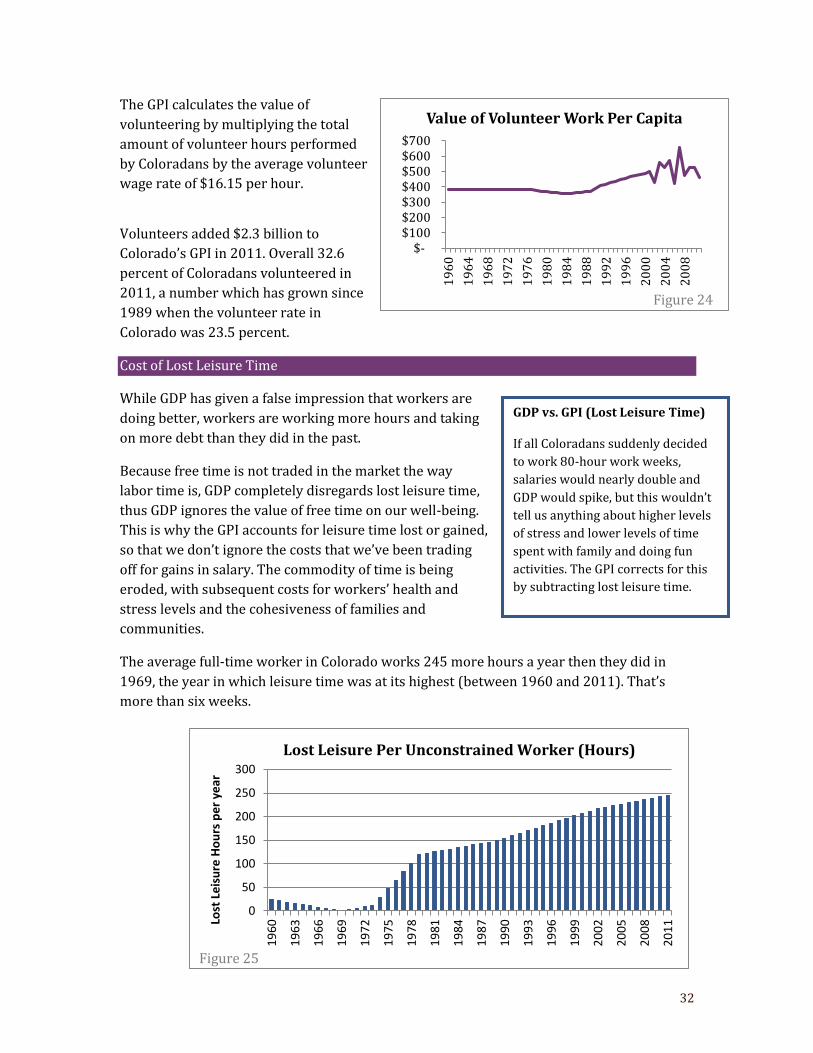
32

The GPI calculates the value of

volunteering by multiplying the total

amount of volunteer hours performed

by Coloradans by the average volunteer

wage rate of $16.15 per hour.

Volunteers added $2.3 billion to

Colorado’s GPI in 2011. Overall 32.6

percent of Coloradans volunteered in

2011, a number which has grown since

1989 when the volunteer rate in

Colorado was 23.5 percent.

Cost of Lost Leisure Time

While GDP has given a false impression that workers are

doing better, workers are working more hours and taking

on more debt than they did in the past.

Because free time is not traded in the market the way

labor time is, GDP completely disregards lost leisure time,

thus GDP ignores the value of free time on our well-being.

This is why the GPI accounts for leisure time lost or gained,

so that we don’t ignore the costs that we’ve been trading

off for gains in salary. The commodity of time is being

eroded, with subsequent costs for workers’ health and

stress levels and the cohesiveness of families and

communities.

The average full-time worker in Colorado works 245 more hours a year then they did in

1969, the year in which leisure time was at its highest (between 1960 and 2011). That’s

more than six weeks.

GDP vs. GPI (Lost Leisure Time)

If all Coloradans suddenly decided

to work 80-hour work weeks,

salaries would nearly double and

GDP would spike, but this wouldn’t

tell us anything about higher levels

of stress and lower levels of time

spent with family and doing fun

activities. The GPI corrects for this

by subtracting lost leisure time.

0

50

100

150

200

250

300

19

60

19

63

19

66

19

69

19

72

19

75

19

78

19

81

19

84

19

87

19

90

19

93

19

96

19

99

20

02

20

05

20

08

20

11Lo

st L

eis

ure

Ho

urs

pe

r ye

ar

Lost Leisure Per Unconstrained Worker (Hours)

Figure 25

$- $100 $200 $300 $400 $500 $600 $700

19

60

19

64

19

68

19

72

19

76

19

80

19

84

19

88

19

92

19

96

20

00

20

04

20

08

Value of Volunteer Work Per Capita

Figure 24

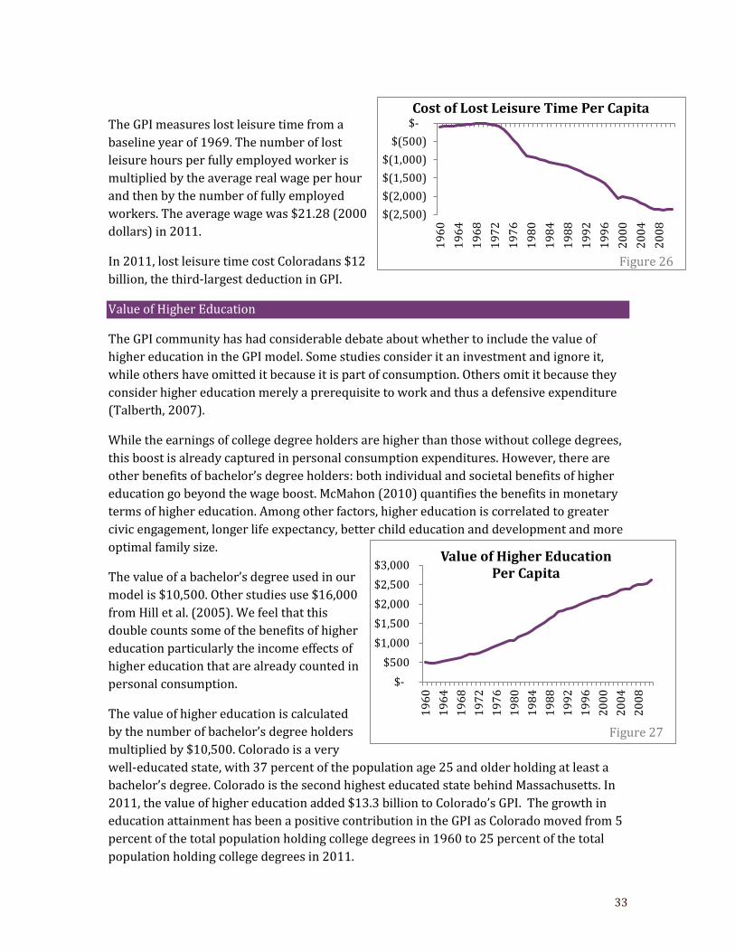
33

The GPI measures lost leisure time from a

baseline year of 1969. The number of lost

leisure hours per fully employed worker is

multiplied by the average real wage per hour

and then by the number of fully employed

workers. The average wage was $21.28 (2000

dollars) in 2011.

In 2011, lost leisure time cost Coloradans $12

billion, the third-largest deduction in GPI.

Value of Higher Education

The GPI community has had considerable debate about whether to include the value of

higher education in the GPI model. Some studies consider it an investment and ignore it,

while others have omitted it because it is part of consumption. Others omit it because they

consider higher education merely a prerequisite to work and thus a defensive expenditure

(Talberth, 2007).

While the earnings of college degree holders are higher than those without college degrees,

this boost is already captured in personal consumption expenditures. However, there are

other benefits of bachelor’s degree holders: both individual and societal benefits of higher

education go beyond the wage boost. McMahon (2010) quantifies the benefits in monetary

terms of higher education. Among other factors, higher education is correlated to greater

civic engagement, longer life expectancy, better child education and development and more

optimal family size.

The value of a bachelor’s degree used in our

model is $10,500. Other studies use $16,000

from Hill et al. (2005). We feel that this

double counts some of the benefits of higher

education particularly the income effects of

higher education that are already counted in

personal consumption.

The value of higher education is calculated

by the number of bachelor’s degree holders

multiplied by $10,500. Colorado is a very

well-educated state, with 37 percent of the population age 25 and older holding at least a

bachelor’s degree. Colorado is the second highest educated state behind Massachusetts. In

2011, the value of higher education added $13.3 billion to Colorado’s GPI. The growth in

education attainment has been a positive contribution in the GPI as Colorado moved from 5

percent of the total population holding college degrees in 1960 to 25 percent of the total

population holding college degrees in 2011.

$-

$500

$1,000

$1,500

$2,000

$2,500

$3,000

19

60

19

64

19

68

19

72

19

76

19

80

19

84

19

88

19

92

19

96

20

00

20

04

20

08

Value of Higher Education Per Capita

Figure 27

$(2,500)

$(2,000)

$(1,500)

$(1,000)

$(500)

$-

19

60

19

64

19

68

19

72

19

76

19

80

19

84

19

88

19

92

19

96

20

00

20

04

20

08

Cost of Lost Leisure Time Per Capita

Figure 26

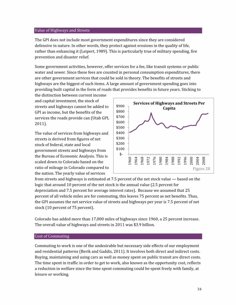
34

Value of Highways and Streets

The GPI does not include most government expenditures since they are considered

defensive in nature. In other words, they protect against erosions in the quality of life,

rather than enhancing it (Leipert, 1989). This is particularly true of military spending, fire

prevention and disaster relief.

Some government activities, however, offer services for a fee, like transit systems or public

water and sewer. Since these fees are counted in personal consumption expenditures, there

are other government services that could be sold in theory. The benefits of streets and

highways are the biggest of such items. A large amount of government spending goes into

providing built capital in the form of roads that provides benefits in future years. Sticking to

the distinction between current income

and capital investment, the stock of

streets and highways cannot be added to

GPI as income, but the benefits of the

services the roads provide can (Utah GPI,

2011).

The value of services from highways and

streets is derived from figures of net

stock of federal, state and local

government streets and highways from

the Bureau of Economic Analysis. This is

scaled down to Colorado based on the

ratio of mileage in Colorado compared to

the nation. The yearly value of services

from streets and highways is estimated at 7.5 percent of the net stock value — based on the

logic that around 10 percent of the net stock is the annual value (2.5 percent for

depreciation and 7.5 percent for average interest rates). Because we assumed that 25

percent of all vehicle miles are for commuting, this leaves 75 percent as net benefits. Thus,

the GPI assumes the net service value of streets and highways per year is 7.5 percent of net

stock (10 percent of 75 percent).

Colorado has added more than 17,000 miles of highways since 1960, a 25 percent increase.

The overall value of highways and streets in 2011 was $3.9 billion.

Cost of Commuting

Commuting to work is one of the undesirable but necessary side effects of our employment

and residential patterns (Berik and Gaddis, 2011). It involves both direct and indirect costs.

Buying, maintaining and using cars as well as money spent on public transit are direct costs.

The time spent in traffic in order to get to work, also known as the opportunity cost, reflects

a reduction in welfare since the time spent commuting could be spent freely with family, at

leisure or working.

$-

$100

$200

$300

$400

$500

$600

$700

$800

$900

19

60

19

64

19

68

19

72

19

76

19

80

19

84

19

88

19

92

19

96

20

00

20

04

20

08

Services of Highways and Streets Per Capita

Figure 28

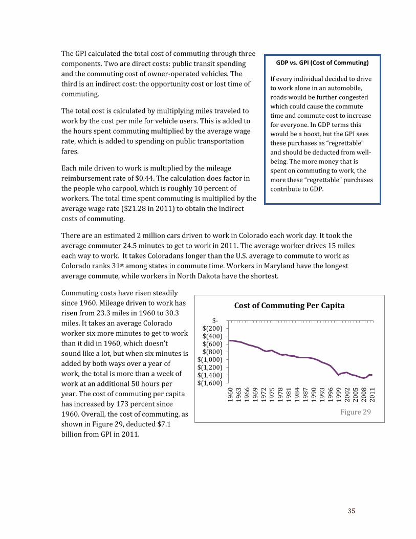
35

The GPI calculated the total cost of commuting through three

components. Two are direct costs: public transit spending

and the commuting cost of owner-operated vehicles. The

third is an indirect cost: the opportunity cost or lost time of

commuting.

The total cost is calculated by multiplying miles traveled to

work by the cost per mile for vehicle users. This is added to

the hours spent commuting multiplied by the average wage

rate, which is added to spending on public transportation

fares.

Each mile driven to work is multiplied by the mileage

reimbursement rate of $0.44. The calculation does factor in

the people who carpool, which is roughly 10 percent of

workers. The total time spent commuting is multiplied by the

average wage rate ($21.28 in 2011) to obtain the indirect

costs of commuting.

There are an estimated 2 million cars driven to work in Colorado each work day. It took the

average commuter 24.5 minutes to get to work in 2011. The average worker drives 15 miles

each way to work. It takes Coloradans longer than the U.S. average to commute to work as

Colorado ranks 31st among states in commute time. Workers in Maryland have the longest

average commute, while workers in North Dakota have the shortest.

Commuting costs have risen steadily

since 1960. Mileage driven to work has

risen from 23.3 miles in 1960 to 30.3

miles. It takes an average Colorado

worker six more minutes to get to work

than it did in 1960, which doesn’t

sound like a lot, but when six minutes is

added by both ways over a year of

work, the total is more than a week of

work at an additional 50 hours per

year. The cost of commuting per capita

has increased by 173 percent since

1960. Overall, the cost of commuting, as

shown in Figure 29, deducted $7.1

billion from GPI in 2011.

GDP vs. GPI (Cost of Commuting)

If every individual decided to drive

to work alone in an automobile,

roads would be further congested

which could cause the commute

time and commute cost to increase

for everyone. In GDP terms this

would be a boost, but the GPI sees

these purchases as “regrettable”

and should be deducted from well-

being. The more money that is

spent on commuting to work, the

more these “regrettable” purchases

contribute to GDP.

$(1,600) $(1,400) $(1,200) $(1,000)

$(800) $(600) $(400) $(200)

$-

19

60

19

63

19

66

19

69

19

72

19

75

19

78

19

81

19

84

19

87

19

90

19

93

19

96

19

99

20

02

20

05

20

08

20

11

Cost of Commuting Per Capita

Figure 29

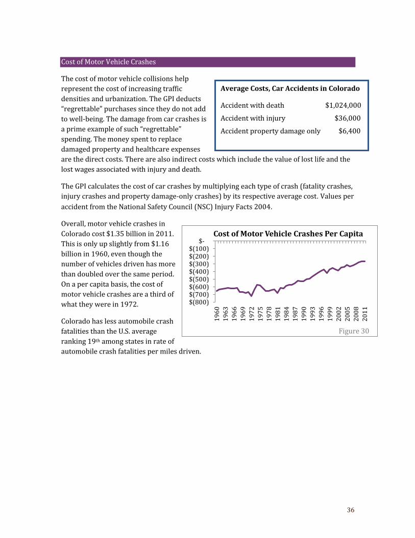
36

Cost of Motor Vehicle Crashes

The cost of motor vehicle collisions help

represent the cost of increasing traffic

densities and urbanization. The GPI deducts

“regrettable” purchases since they do not add

to well-being. The damage from car crashes is

a prime example of such “regrettable”

spending. The money spent to replace

damaged property and healthcare expenses

are the direct costs. There are also indirect costs which include the value of lost life and the

lost wages associated with injury and death.

The GPI calculates the cost of car crashes by multiplying each type of crash (fatality crashes,

injury crashes and property damage-only crashes) by its respective average cost. Values per

accident from the National Safety Council (NSC) Injury Facts 2004.

Overall, motor vehicle crashes in

Colorado cost $1.35 billion in 2011.

This is only up slightly from $1.16

billion in 1960, even though the

number of vehicles driven has more

than doubled over the same period.

On a per capita basis, the cost of

motor vehicle crashes are a third of

what they were in 1972.

Colorado has less automobile crash

fatalities than the U.S. average

ranking 19th among states in rate of

automobile crash fatalities per miles driven.

Average Costs, Car Accidents in Colorado

Accident with death $1,024,000

Accident with injury $36,000

Accident property damage only $6,400

$(800) $(700) $(600) $(500) $(400) $(300) $(200) $(100)

$-

19

60

19

63

19

66

19

69

19

72

19

75

19

78

19

81

19

84

19

87

19

90

19

93

19

96

19

99

20

02

20

05

20

08

20

11

Cost of Motor Vehicle Crashes Per Capita

Figure 30

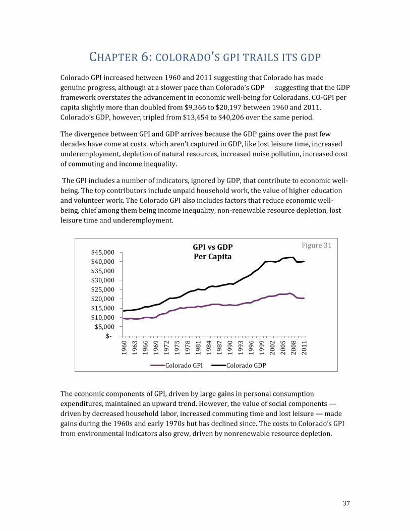
37

CHAPTER 6: COLORADO’S GPI TRAILS ITS GDP

Colorado GPI increased between 1960 and 2011 suggesting that Colorado has made

genuine progress, although at a slower pace than Colorado’s GDP — suggesting that the GDP

framework overstates the advancement in economic well-being for Coloradans. CO-GPI per

capita slightly more than doubled from $9,366 to $20,197 between 1960 and 2011.

Colorado’s GDP, however, tripled from $13,454 to $40,206 over the same period.

The divergence between GPI and GDP arrives because the GDP gains over the past few

decades have come at costs, which aren’t captured in GDP, like lost leisure time, increased

underemployment, depletion of natural resources, increased noise pollution, increased cost

of commuting and income inequality.

The GPI includes a number of indicators, ignored by GDP, that contribute to economic well-

being. The top contributors include unpaid household work, the value of higher education

and volunteer work. The Colorado GPI also includes factors that reduce economic well-

being, chief among them being income inequality, non-renewable resource depletion, lost

leisure time and underemployment.

The economic components of GPI, driven by large gains in personal consumption

expenditures, maintained an upward trend. However, the value of social components —

driven by decreased household labor, increased commuting time and lost leisure — made

gains during the 1960s and early 1970s but has declined since. The costs to Colorado’s GPI

from environmental indicators also grew, driven by nonrenewable resource depletion.

$-

$5,000

$10,000

$15,000

$20,000

$25,000

$30,000

$35,000

$40,000

$45,000

19

60

19

63

19

66

19

69

19

72

19

75

19

78

19

81

19

84

19

87

19

90

19

93

19

96

19

99

20

02

20

05

20

08

20

11

GPI vs GDPPer Capita

Colorado GPI Colorado GDP

Figure 31

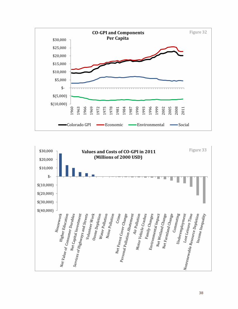
38

$(10,000)

$(5,000)

$-

$5,000

$10,000

$15,000

$20,000

$25,000

$30,000

19

60

19

63

19

66

19

69

19

72

19

75

19

78

19

81

19

84

19

87

19

90

19

93

19

96

19

99

20

02

20

05

20

08

20

11

CO-GPI and ComponentsPer Capita

Colorado GPI Economic Environmental Social

Figure 32

$(40,000)

$(30,000)

$(20,000)

$(10,000)

$-

$10,000

$20,000

$30,000 Values and Costs of CO-GPI in 2011(Millions of 2000 USD)

Figure 33

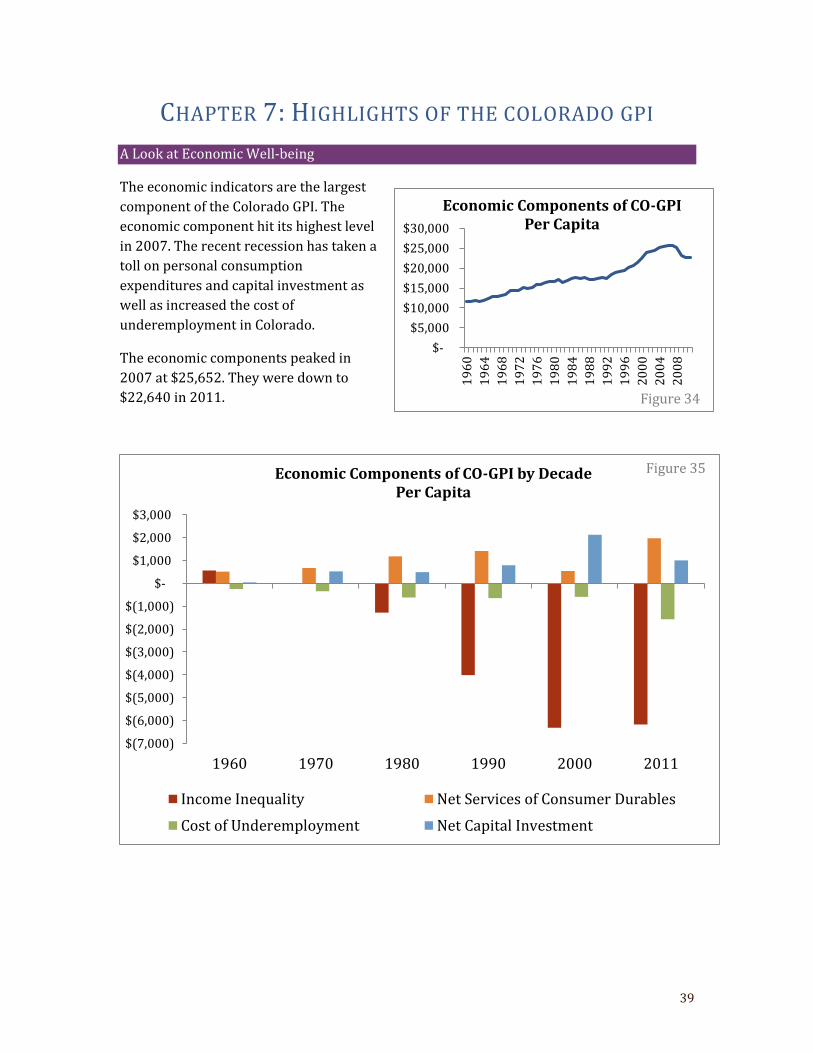
39

CHAPTER 7: HIGHLIGHTS OF THE COLORADO GPI

A Look at Economic Well-being

The economic indicators are the largest

component of the Colorado GPI. The

economic component hit its highest level

in 2007. The recent recession has taken a

toll on personal consumption

expenditures and capital investment as

well as increased the cost of

underemployment in Colorado.

The economic components peaked in

2007 at $25,652. They were down to

$22,640 in 2011.

$(7,000)

$(6,000)

$(5,000)

$(4,000)

$(3,000)

$(2,000)

$(1,000)

$-

$1,000

$2,000

$3,000

1960 1970 1980 1990 2000 2011

Economic Components of CO-GPI by DecadePer Capita

Income Inequality Net Services of Consumer Durables

Cost of Underemployment Net Capital Investment

Figure 35

$-

$5,000

$10,000

$15,000

$20,000

$25,000

$30,000

19

60

19

64

19

68

19

72

19

76

19

80

19

84

19

88

19

92

19

96

20

00

20

04

20

08

Economic Components of CO-GPIPer Capita

Figure 34

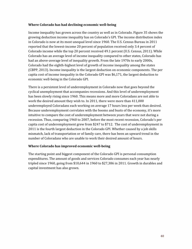
40

Where Colorado has had declining economic well-being

Income inequality has grown across the country as well as in Colorado. Figure 35 shows the

growing deduction income inequality has on Colorado’s GPI. The income distribution index

in Colorado is now at its most unequal level since 1960. The U.S. Census Bureau in 2011

reported that the lowest-income 20 percent of population received only 3.4 percent of

Colorado income while the top 20 percent received 49.1 percent (U.S. Census, 2011). While

Colorado has an average level of income inequality compared to other states, Colorado has

had an above-average level of inequality growth. From the late 1970s to early 2000s,

Colorado had the eighth-highest level of growth of income inequality among the states

(CBPP, 2013). Income inequality is the largest deduction on economic components. The per

capita cost of income inequality in the Colorado GPI was $6,171, the largest deduction to

economic well-being in the Colorado GPI.

There is a persistent level of underemployment in Colorado now that goes beyond the

cyclical unemployment that accompanies recessions. And this level of underemployment

has been slowly rising since 1960. This means more and more Coloradans are not able to

work the desired amount they wish to. In 2011, there were more than 411,000

underemployed Coloradans each working on average 17 hours less per week than desired.

Because underemployment correlates with the booms and busts of the economy, it’s more

intuitive to compare the cost of underemployment between years that were not during a

recession. Thus, comparing 1960 to 2007, before the most recent recession, Colorado’s per

capita cost of underemployment grew from $247 to $712. The cost of underemployment in

2011 is the fourth largest deduction in the Colorado GPI. Whether caused by a job skills

mismatch, lack of transportation or of family care, there has been an upward trend in the

number of Coloradans who are unable to work their desired amount of hours.

Where Colorado has improved economic well-being

The starting point and biggest component of the Colorado GPI is personal consumption

expenditures. The amount of goods and services Colorado consumes each year has nearly

tripled since 1960, going from $10,644 in 1960 to $27,386 in 2011. Growth in durables and

capital investment has also grown.

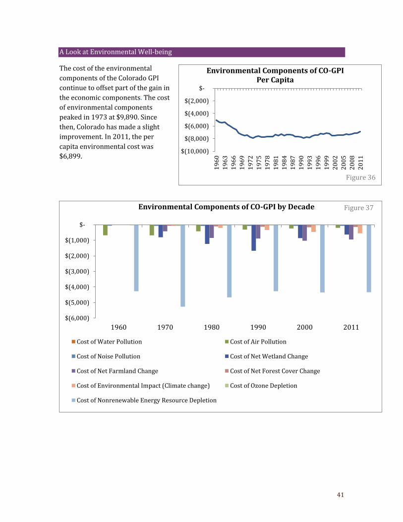
41

A Look at Environmental Well-being

The cost of the environmental

components of the Colorado GPI

continue to offset part of the gain in

the economic components. The cost

of environmental components

peaked in 1973 at $9,890. Since

then, Colorado has made a slight

improvement. In 2011, the per

capita environmental cost was

$6,899.

$(6,000)

$(5,000)

$(4,000)

$(3,000)

$(2,000)

$(1,000)

$-

1960 1970 1980 1990 2000 2011

Environmental Components of CO-GPI by Decade

Cost of Water Pollution Cost of Air Pollution

Cost of Noise Pollution Cost of Net Wetland Change

Cost of Net Farmland Change Cost of Net Forest Cover Change

Cost of Environmental Impact (Climate change) Cost of Ozone Depletion

Cost of Nonrenewable Energy Resource Depletion

Figure 37

$(10,000)

$(8,000)

$(6,000)

$(4,000)

$(2,000)

$-

19

60

19

63

19

66

19

69

19

72

19

75

19

78

19

81

19

84

19

87

19

90

19

93

19

96

19

99

20

02

20

05

20

08

20

11

Environmental Components of CO-GPIPer Capita

Figure 36

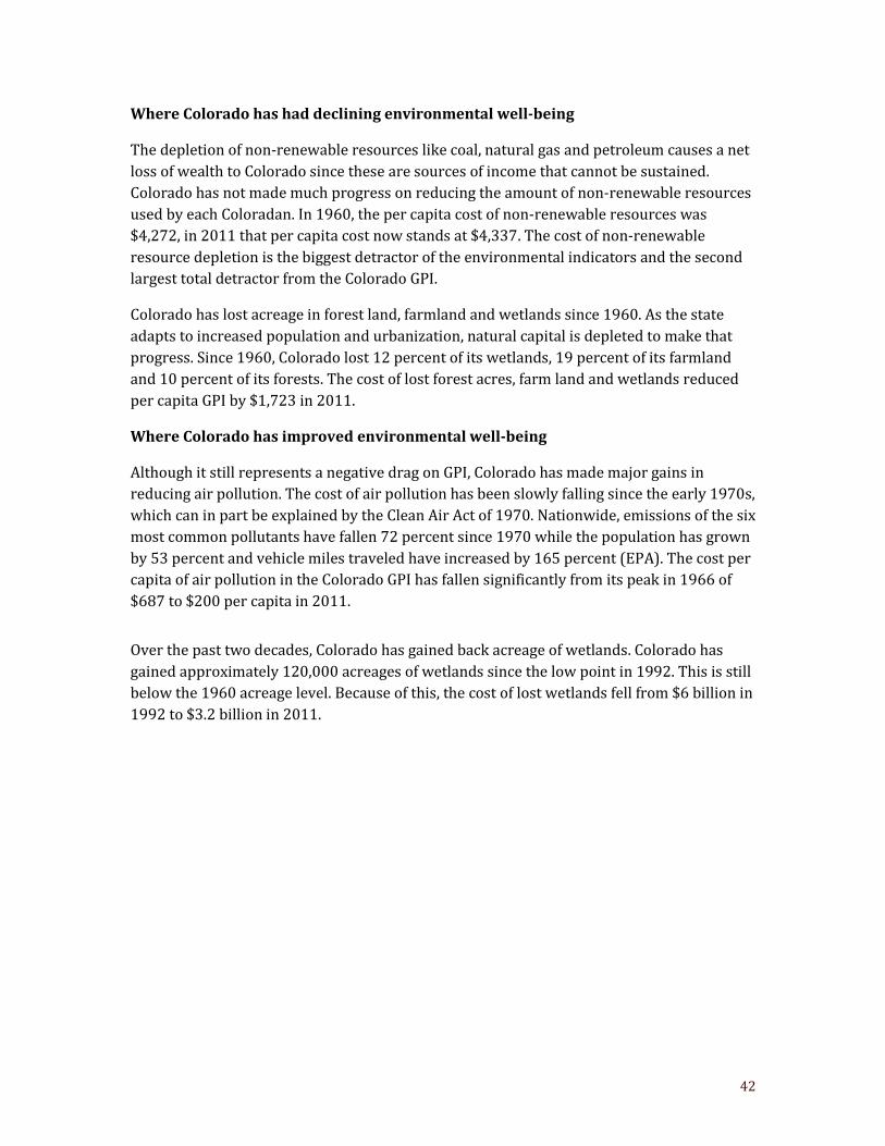
42

Where Colorado has had declining environmental well-being

The depletion of non-renewable resources like coal, natural gas and petroleum causes a net

loss of wealth to Colorado since these are sources of income that cannot be sustained.

Colorado has not made much progress on reducing the amount of non-renewable resources

used by each Coloradan. In 1960, the per capita cost of non-renewable resources was

$4,272, in 2011 that per capita cost now stands at $4,337. The cost of non-renewable

resource depletion is the biggest detractor of the environmental indicators and the second

largest total detractor from the Colorado GPI.

Colorado has lost acreage in forest land, farmland and wetlands since 1960. As the state

adapts to increased population and urbanization, natural capital is depleted to make that

progress. Since 1960, Colorado lost 12 percent of its wetlands, 19 percent of its farmland

and 10 percent of its forests. The cost of lost forest acres, farm land and wetlands reduced

per capita GPI by $1,723 in 2011.

Where Colorado has improved environmental well-being

Although it still represents a negative drag on GPI, Colorado has made major gains in

reducing air pollution. The cost of air pollution has been slowly falling since the early 1970s,

which can in part be explained by the Clean Air Act of 1970. Nationwide, emissions of the six

most common pollutants have fallen 72 percent since 1970 while the population has grown

by 53 percent and vehicle miles traveled have increased by 165 percent (EPA). The cost per

capita of air pollution in the Colorado GPI has fallen significantly from its peak in 1966 of

$687 to $200 per capita in 2011.

Over the past two decades, Colorado has gained back acreage of wetlands. Colorado has

gained approximately 120,000 acreages of wetlands since the low point in 1992. This is still

below the 1960 acreage level. Because of this, the cost of lost wetlands fell from $6 billion in

1992 to $3.2 billion in 2011.

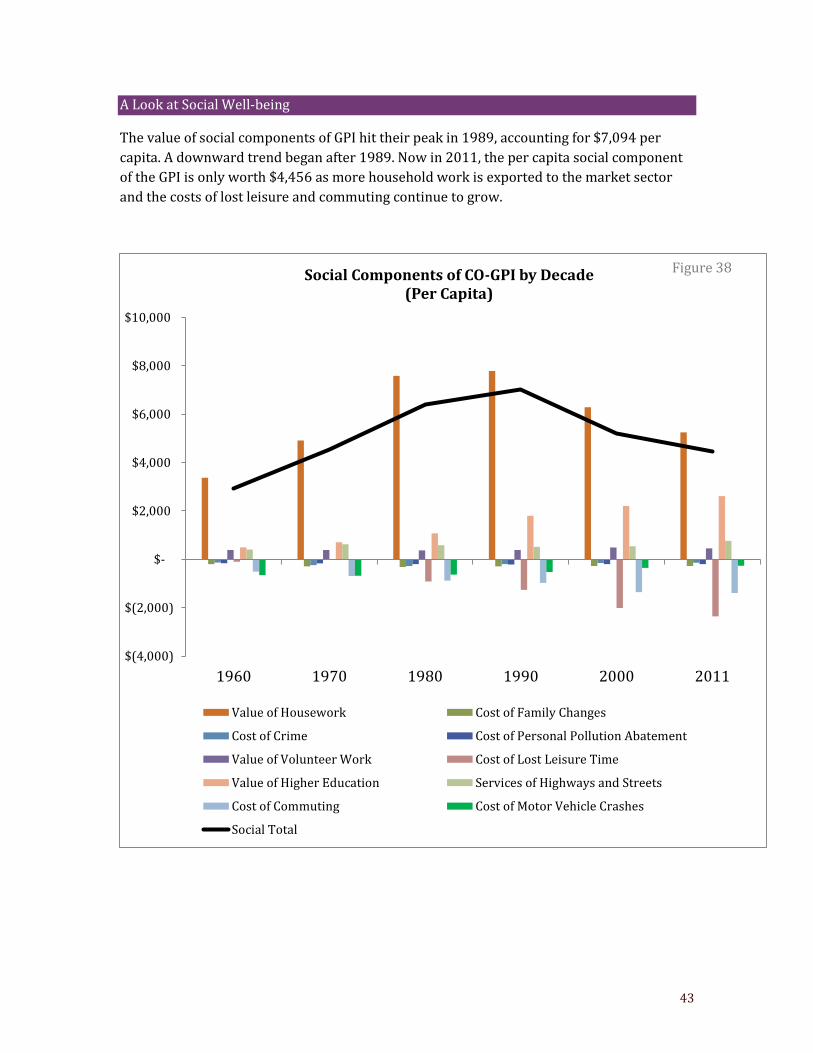
43

A Look at Social Well-being

The value of social components of GPI hit their peak in 1989, accounting for $7,094 per

capita. A downward trend began after 1989. Now in 2011, the per capita social component

of the GPI is only worth $4,456 as more household work is exported to the market sector

and the costs of lost leisure and commuting continue to grow.

$(4,000)

$(2,000)

$-

$2,000

$4,000

$6,000

$8,000

$10,000

1960 1970 1980 1990 2000 2011

Social Components of CO-GPI by Decade(Per Capita)

Value of Housework Cost of Family Changes

Cost of Crime Cost of Personal Pollution Abatement

Value of Volunteer Work Cost of Lost Leisure Time

Value of Higher Education Services of Highways and Streets

Cost of Commuting Cost of Motor Vehicle Crashes

Social Total

Figure 38

44

Where Colorado has had declining social well-being

Because GDP focuses only on market transactions, it ignores the value of free time on our

well-being. The biggest weight on the social components of GPI come from the cost of lost

leisure time. The cost of lost leisure began to grow around 1980. The average full-time

worker in Colorado works 245 more hours a year then they did in 1969, the year in which

leisure time was at its highest (between 1960 and 2011). That’s more than six weeks.

The cost of commuting has become a growing weight on Colorado’s well-being. Commuting

costs have risen steadily since 1960. Mileage driven to work has risen from 23.3 miles in

1960 to 30.3 miles. It takes an average Colorado worker six more minutes to get to work

than it did in 1960. The cost of commuting per capita has increased by 173 percent since

1960.

The biggest contribution to social well-being in the Colorado GPI is household work. The

value of household work per capita peaked in 1986 at $8,004. The decline in the value of

household labor over the past few decades should not be viewed as total negative, but

should be viewed as an adjustment to the well-being in earlier years when most of

household labor was done outside the market and not counted in personal consumption or

GDP. Since many Coloradans began exporting more and more household work to the market

(in the form of appliances, paying for household services and meals) the value of this gets

captured in personal consumption.

Where Colorado has improved social well-being

The value of higher education has been a growing positive. The value of higher education in

the Colorado GPI has growth by more than a factor of five since 1960 as more and more

Coloradans are obtaining college degrees. In 1960, 5 percent of the Colorado population had

a bachelor’s degree or higher. In 2011, 25 percent had a bachelor’s degree or higher.

Colorado is the second most educated state in the country.

The cost of motor vehicles accidents has also improved over the past few decades. Since the

peak in 1972, the cost of motor vehicle accidents per capita has fallen dramatically. In 2011,

the cost of motor vehicle crashes were a third of that they were in 1972.

Although the cost of crime in Colorado rose considerably in the 1960s, peaking in 1981, this

cost was cut in half between 1981 and 2011.

45

REFERENCES

Alternative Flurocarbons Environmental Acceptability Study (AFEAS). (2006). Production,

sales and emissions statistics. Available at http://www.afeas.org/

American Association of Automobile Manufacturers. (1996). 1996 Motor Vehicle Facts and

Figures. Detroit: Government Affairs Division of the American Automobile

Manufacturers Association.

Anielski, M. & Rowe, J. (1999). The Genuine Progress Indicator—1998 Update. Oakland CA:

Redefining Progress.

Bagstad, K. J. & Shammin, M.R. (2012). Can the Genuine Progress Indicator better inform

sustainable regional progress—A case study for Northeast Ohio. Ecological

Indicators, 18, 300-341.

Bagstad, K. J. & Ceroni, M. (2007). Opportunities and challenges in applying the Genuine

Progress Indicator/Index of Sustainable Economic Welfare at local scales.

International Journal of Environment, Workplace, and Employment, Vol. 3, No.2,

132-153.

Baumgärtner, S. & Quaas, M.F. (2009). Ecological‐economic viability as a criterion of strong

sustainability under uncertainty. Ecological Economics 2008 – 2020, 68.

Berik, G. & Gaddis, E. (2011). The Utah Genuine Progress Indicator, 1990 to 2007: A report

to the people of Utah. Available at http://www.dnr.maryland.gov/mdgpi/pdfs/GPI-

Utah.pdf.

Bernstein, M & Schmitt, J. (1996). The State of Working America 1995-1996. New York:

Sharpe, Armink. Burakowski, E. & Magnusson, M. (2012) Climate Impacts and the

Winter Tourism Economy in the United States. Available at

http://www.nrdc.org/globalwarming/files/climate-impacts-winter-tourism-

report.pdf.

Breen, R. (1997). Inequality, economic growth and social mobility. The British

Journal of Sociology, 48, 3, 429 – 449.

Center on Budget and Policy Priorities. (2012). Pulling Apart: A state‐by –state analysis of

income trends. Available at http://www.cbpp.org/cms/?fa=view&id=3860

Cobb, C., & Cobb, J. B Jr., EDS. (1994). The Green National Product: A Proposed Index of

Sustainable Economic Welfare. Lanham, MD: University Press of America.

46

Cobb, C., Halstead, T., & Rowe, J. (1995). The Genuine Progress Indicator: Summary of Data

and Methodology. Oakland CA: Redefining Progress.

Congressional Quarterly, Inc. (1972). Congressional Quarterly Almanac. Washington, DC:

Congressional Quarterly, Inc.

Costanza, R., Erikson, J., Fligger, K., Adams, A., Christian, A., Atschuler, B., Balter, S., Fisher, B.,

Hike, J., Kelly, J., Kerr, T., McCauley, M., Montone, K., Rauch, M., Schmiedeskamp, K.,

Saxton, D., Sparacino, L., Tusinski, W., and Williams, L. 2004.

Estimates of the Genuine Progress Indicator (GPI) for Vermont, Chittenden County

and Burlington, from 1950 to 2000. Ecological Economics, 51: 139 – 155.

Daly, H., & Cobb, J. (1990). For the Common Good: Redirecting the economy toward

community, the environment, and a sustainable future. Boston, MA: Beacon Press.

Daly, H.E. & Farley, J. 2004. Ecological Economics: Principles and Applications.

Washington DC: Island Press

Deininger, K & Squire, S. (1998). New ways of looking at old issues: inequality and

growth. Journal of Development Economics, 57, 2, 259-287.

Dodds, W.K., Wilson, K.C., Rehmeier, R.L., Knight, G.L., Wiggam, S., Falke, J.A., Dalgleish, H.J. &

Bertrand, K.N. (2008). Comparing ecosystem goods and services provided by

restored and native lands. BioScience, 58, 9, 837 – 845.

Doesken, N. (2007) Colorado Climate Center. Presentation available at

http://ccc.atmos.colostate.edu/pdfs/Nolan_TempInversions--

Colorado(Jan9_2007)%20v2.pdf

Easterlin, R. (1974). Does economic growth improve the human lot? In David, P., and

Weber, R. (eds.) Nations and Households in Economic Growth. New York:

Academic Press.

Environmental Protection Agency. (2013). Air Pollution and the Clean Air Act. Available at

http://www.epa.gov/air/caa/

Fisher, I. (1906). The Nature of Capital and Income. New York: Macmillian.

Frank, R. (2000). “Does growing inequality harm the middle class?” Eastern

Economic Journal, 26, 3, 253-264.

47

Frank, M. (2008). A New State-Level Panel of Income Inequality Measures Over the Period

1916-2005. Sam Houston State University Working Paper Series. Available at

http://www.shsu.edu/~tcq001/paper_files/wp08-02_paper.pdf

Franklin Associates. (1997). Solid Waste Management at the Crossroads. Available at

http://www.zerowasteamerica.org/EconomicsOfWaste.htm

Freeman, M. (1982). Air and Water Pollution control: A benefit cost analysis. New York:

John Wiley and Sons.

Furman, J. & Stiglitz, J. (1998). Economic consequences of income inequality. Income

Inequality: Issues and Policy Options–Proceedings of a Symposium Sponsored by the

Federal Reserve Bank of Kansas City. Available at

http://www.kc.frb.org/PUBLICAT/SYMPOS/1998/S98stiglitz.pdf

Georgopoulos, D., Papadogonas, T., & Sfakianakis, G. (2010).

Inequality/Poverty and the 'Great Recession': The case of the 27 members states of

the European Union.

Ghermandi, A., van den Bergh, J.C.J.M., Brander, L.M., de Groot, H.L.F., & Nunes, P A.L.D.

(2008). The economic value of wetland conservation and creation: A meta‐analysis.

The Berkeley Electronic Press, 238.

Hagerty, M., Cummins, R.A, Ferriss, A.L., Land, K., Michalos, A.C., Peterson, M. Sharpe, A.,

Sirgy, J. & Vogel, J. (2001). Quality of life indexes for national policy: review and

agenda for research. Social Indicators Research, 55, 1‐96.

Hawaii State Environmental Council (2013). “Towards a Green Economy; Introducing the

GPI to Hawaii.” Annual Report.

Hill, K., Hoffman, D. & Rex, T.R. (2005). The Value of Higher Education:

Individual and Societal Benefits. Tempe, Arizona: Arizona State University, W.P.

Carey School of Business.

Hsing, Yu. (2006). “Economic growth and income inequality; the case of the U.S.”

International Journal of Social Economics. 32, 7, 639-647.

Holt, R. F., & Greenwood, D. T. (2012). Negative Trickle-Down and the Financial

Crisis of 2008. Journal Of Economic Issues (M.E. Sharpe Inc.), 46(2), 363-370.

Iceland, J. (2003). Why poverty remains high: The role of income growth,

economic inequality and changes in family structure, 1949-1999. Demography, 40, 3,

499-519.

48

Katz, A. J. (1983). Valuing the services of consumer durables. The Review of Income and

Wealth, (Series 29). Available at http://roiw.org/1983/405.pdf

Kirkorian, H.L., Pempek, T.A., Murphy, L.A., Schmidt, M.E., & Anderson, D.R. (2009). The

impact of background television on parent‐child interaction.

Child Development, 80, 1350‐1359.

Kuznets, S. (1934). National Income 1929–1932. A report to the U.S. Senate, 73rd Congress,

2nd Session. Washington, DC: U.S. Government Printing Office.

Kuznets, S., Epstein, L., & Jenks, E. (1941). National Income and Its Composition, 1919–1938,

Volume 1. New York: National Bureau of Economic Research.

Landefeld, J. S., Siskin, E.P, & Fraumeni, B.M. (2008). Taking the pulse of the economy:

Measuring GDP. Journal of Economic Perspectives, 22, 2, 193‐216.

Lawn, P. (2005). An assessment of the valuation methods used to calculate the Index of

Sustainable Economic Welfare (ISEW), Genuine Progress Indicator (GPI), and

Sustainable Net Benefit Index (SNBI). Environment, Development and Sustainability,

7, 185‐208.

Leipert, Christian. (1989). National income and economic growth: the conceptual side of

defensive expenditures. Journal of Economic Issues 23,3, 843-856.

Makhijani, A. (2007). Carbon-free and nuclear-free. A roadmap for U.S. energy policy.

Takoma, MD: IEER Press.

McMahon, W.W. (2010). The Private and Societal Benefits of Higher Education: The

Evidence, Their Value, and Policy Implications. TIAA-CREF Institute. Available at:

http://www1.tiaacref.org/ucm/groups/content/@ap_ucm_p_tcp_docs/documents/

document/tiaa02029326.pdf

Millennium Ecosystem Assessment (MEA). (2005). Ecosystems and human well‐being.

Washington, DC: Island Press.

Mitsch, William J. and Gosselink, James C. (2007) Wetlands. New Jersey:

John Wiley & Sons, Inc.

Moretti, E. (2004). Estimating the social return to higher education: evidence from

longitudinal and repeated cross-sectional data. Journal of Econometrics, July/

August, 175-212.

49

Muller, N.Z. & Mendelsohn, R. (2007). Measuring the damages of air pollution in the United

States. Journal of Environmental Economics and Management, 54, 1 – 14.

National Safety Council. (2004). Estimating the Costs of Unintentional Injuries, 2000.

Norton, Michael I. and Ariely, Dan. (2011). “Building a Better America—One Wealth Quintile

at a Time.” Perspectives on Psychological Science 6: 9

Pearce, D.W (1994). Assessing the Social Rate of Return from Investment in Temperate

Zone Forestry, in R. Layard and S. Glaister (eds), Cost-Benefit Analysis, 2nd edition,

Cambridge: Cambridge University Press, 464-490.

Pearce, D.W. (2001). The Economic Value of Forest Ecosystems. Available at

http://www.cbd.int/doc/external/academic/forest-es-2003-en.pdf

Pederson, G. T., Betancourt, J. L. & McCabe, G. J. (2013). Regional patterns and proximal

causes of the recent snowpack decline in the Rocky Mountains. Geographical

Research Letters, 40, 9, 1811-1816.

Posner, S.M. (2010). Estimating the Genuine Progress Indicator for Baltimore, MD. Master’s of

Science Thesis, University of Vermont, Burlington.

Reich, R. (2010). Aftershock: The next economy and America’s future. New York:

Random House, LLC.

Sen, A.K. (1997). Inequality, unemployment, and contemporary Europe. International

Labour Review, 136, 2, 155‐172.

Stiglitz, Joseph E. (2013). Inequality is Holding Back the Recovery. The New York Times.

Available at

http://opinionator.blogs.nytimes.com/2013/01/19/inequality-is- holding-back-

the-recovery/

Talberth, J., Cobb, C., & Slattery, N. (2007). The Genuine Progress Indicator 2006: A tool for

sustainable development. Oakland, CA: Redefining Progress.

Temperature Inversions. (2013). Sky View Weather. Available at

http://www.skyviewweather.com/learning/temperature-inversions/

Todaro, M. & Smith S. (2009). Economic Development, Tenth Edition. Pearson Higher Ed.

50

Tol, R.S.J. (2005). The Marginal Damage Costs of Carbon Dioxide Emissions: An Assessment

of the Uncertainties. Energy Policy, 33, 2064‐2074.

US Census Data. (2011). Shares of Aggregate household income by quintile for Colorado

[Data File]. Retrieved from

http://factfinder2.census.gov/faces/tableservices/jsf/pages/productview.xhtml?pi

d=ACS_11_3YR_B19082&prodType=table

Venetoulis, J., & Cobb, C. (2004). The Genuine Progress Indicator 1950-2002 (2004 Update).

Oakland, California: Redefining Progress.

Venetoulis, J., & Talberth, T. (2006). Refining the ecological footprint. Environment,

Development, and Sustainability, 10, 4, 441-469.

Wang, W. (2013). “Parents’ Time with Kids More Rewarding than Paid Work—and More

Exhausting.” Pew Research Center. Available at

http://www.pewsocialtrends.org/files/2013/10/parental-time-use_10-2013.pdf

Wilkinson, Richard G. and Kate Pickett. 2010. The spirit level: why greater equality

makes societies stronger. New York: Bloomsbury Press.

Wisman, J. D. (2011). Inequality, social respectability, political power, and

environmental devastation. Journal of Economic Issues, 45,(4), 877-900.

Wisman, J. D. (2013). Wage stagnation, rising inequality and the financial

crisis of 2008. Cambridge Journal of Economics.

Wolfinger, N.H. (2005). Understanding the Divorce Cycle: The Children of Divorce in Their

Own Marriages. NY: Cambridge University Press.

Zolotas, X. (1981). Economic Growth and Declining Social Welfare. New York: New York

University Press.

51

APPENDIX A: DETAILED METHODS OF COLORADO’S GPI Personal Consumption

The values for personal income since 1960 were obtained from the U.S. Bureau of Economic

Analysis Regional Economic Accounts, found here:

http://bea.gov/iTable/iTable.cfm?ReqID=70&step=1#reqid=70&step=1&isuri=1.

The percentage of income that goes toward consumption was estimated using the National

Income and Product Accounts, 2.1 Personal Income and its Disposition, found here:

http://bea.gov/iTable/iTable.cfm?ReqID=9&step=1#reqid=9&step=1&isuri=1. This method

assumes that the rate of consumption in Colorado is the same as the national rate since

consumption data is not available at the state level.

Income Distribution

Finding income inequality data at the state level is difficult. Other GPI studies use IRS data

which has a limitation because of the omission of people whose earnings are less than a

threshold level of income. Using IRS data, researchers generally focus on the top-income

earner shares. Non-IRS data does not have this problem but the data is not available

annually. For instance, the decennial census income data is only available every ten years.

Only recently has the Current Population Survey provided Gini numbers for years 2006

forward.

Other GPI studies have used Nielsen’s (1997) methodology for decennial years and used

national data to piece together state level inequality numbers. Instead of extrapolating

decennial data, which we view as less accurate, we use Frank (2008). The author calculates

five measures of inequality (Atkinson Index, Gini Coefficient, Relative Mean Deviation, Theil

Index, Top 10% and Top 1%) for each state up till 2005. You can find the data from Sam

Houston State University here: http://www.shsu.edu/eco_mwf/inequality.html. Years 2006 and

forward we rely on the U.S. Census Bureau’s Gini figures.

In order to splice the CPS data with Frank’s data from 1960-2005 we had to pair-down

Frank’s data to fit into the Census Bureau’s data. (Franks Gini index for 2005 was .58 and

Census Bureau’s was .45). We reduced Frank’s series by a factor of (.45/.58) in order to

preserve the inequality ratio and thus be able to use Census Bureau’s numbers for future

years.

Next we index these inequality coefficients setting 1970 as the base year like other GPI

studies since the U.S. experienced its lowest level of inequality that year. An index allows us

to show relative change from year to year.

Personal Consumption Adjusted for Income Inequality

Personal consumption is adjusted for income inequality by dividing personal consumption

by the income distribution index and multiplying by 100.

52

Services of Consumer Durables

The GPI views the original purchase price of consumer durables as a cost, and the

services a consumer received from the product over its lifetime as a benefit. Like other GPI

studies, the average consumer capital item is assumed to last 8 years which translates into a

fixed depreciation rate of 12.5 percent. The Cost of Consumer Durables is used to impute

that service of consumer durables. Added to the depreciation rate is the average interest

rate of 7.5 percent. This is based on the fact that consumers could, instead of purchasing

consumer durables, have invested their money at this interest rate. So the stock of durables

is multiplied by a factor of 20 percent to get each year’s services of those durables.

Cost of Consumer Durables

Data of spending on durables is not available at the state level, but is available at the

national level from Bureau of Economic Analysis NIPA Table 2.3.5. The percentage of

personal income spent on durable goods for the U.S. was used to calculate Colorado’s

spending on durables. This ratio was multiplied by person income in Colorado.

Cost of Underemployment

The total cost of underemployment equals the number of underemployed people multiplied

by the hours of unprovided work per underemployed worker multiplied by average real

wage rate.

All three factors needed to be calculated for Colorado. The Bureau of Labor Statistics began

publishing underemployment state data in 2003. For prior years the unemployment rate

was adjusted by a quadratic relationship, used by Costanza et al. (2004), to impute

underemployment rate. The quadratic equation was developed via a regression using

Schor’s (1997) data, BLS data and another data point based on an assumption that if there is

full unemployment, there would also have to be full underemployment as well.

The quadratic equation is: % (underemployed + unemployed) = -

0.000087305*(100*Unemployment%)^2) + 0.969325*(100*Unemployment%)) +

3.941336.

Unprovided hours per underemployed worker come from Leete-Guy and Schor (1992).

Extrapolation was used to compute the other year. Before 1969 and beyond 1989, the

national and previous State GPI studies used the assumption of a continued growth of

yearly unprovided hours by 0.59 percent per year.

Average hourly wage calculated by dividing employee compensation from BEA by

employees, by weeks per year and by average hours worked per week. The same average

real wage rate is used in the lost leisure indicator.

53

Net Capital Investment

The GPI calculates changes in the stock of capital by adding the amount of new capital stock

(net stock of private nonresidential fixed reproducible capital from the BEA) and

subtracting the capital requirement, which is the amount that maintains the same level of

capital per worker. To calculate a capital requirement, the percent change in labor force

each year is applied to the stock of capital. In order to smooth out yearly fluctuations, a five-

year rolling average of changes in labor force and capital was used. Since State data was not

available, national data was scaled down by population.

Cost of Water Pollution

To calculate trends in water pollution for Colorado, we used the 305(b) report on water

quality from the Colorado Department of Public Health and Environment. The 2008 report

had the highest percentage of assessed rivers and stream since their assessment methods

changed in 2004. Using 2008 as the base year, figures for other years were estimated using

the trends used by Costanza et al. (2004). Earlier years were interpolated following an

assumption that water quality declined by 3 percent each year since there was no pollution

control regulations in place then (years 1960-1972). A stable water quality level was

assumed for 1973-1990 and a 2 percent per year improvement in water quality was

assumed for 1991 to 2011. These trends were applied to the percentage impairments ratio,

therefore a decline in water quality means an increase in the percent of water impaired.

We followed Maryland’s GPI methodology for calculating the per capita value of clean water.

Drawing on a review of a number of valuation studies, a value of $130 dollars per capita, or

$562.5 million overall, in 2000 for clean water was adopted. The cost of water pollution is

simply the value of clean water multiplied by the percentage of rivers and lakes that are

impaired.

Cost of Air Pollution

Tons of pollution emitted in Colorado was obtained from the National Emissions Inventory

Database provided by the Environmental Protection Agency, which provides detailed

emissions data for various pollutants at the state level since 1990.

http://www.epa.gov/ttn/chief/eiinformation.html.

National EPA emissions trends from 1970 to 1990 were used to estimate Colorado’s

emissions which can be found

http://www.epa.gov/ttn/chief/trends/trends06/national_tier1_caps.xlsx.

For figures prior to 1970, Aneilski and Rowe’s (1999) assumptions were used: air quality

declined 2.4 percent per year in the 1960s. .

The cost per ton of pollution was drawn from Muller and Mendelsohn (2007), in which the

authors estimated the marginal damage associated with emitting an additional ton of six

different pollutants (ammonia, nitrogen dioxide, PM10, PM2.5, sulfur dioxide and volatile

organic compounds). Most of the damage associated with air pollution comes from

premature mortalities. Overall reductions in health account for 94 percent of the total

damages of air pollution. The remaining 6 percent come from visibility loss, reduced

54

agricultural yield, reduced timber yield, accelerated depreciation of man-made material and

impaired forest health. The per ton damages of NOX was $273 in 2000 dollars. PM10

damages were $544 per ton. PM2.5 damages were $3462 per ton. SO2 damages were $1261

per ton. VOC was $676 per ton.

Cost of Noise Pollution

National Data was scaled down based on Colorado’s urban population, where noise effects

are most likely to occur. Like other state GPI studies, we use a national cost of $14.62 billion

for noise pollution in 1972 from an old WHO study. This estimate was extrapolated

following Bagstad and Ceroni (2007) based on increases in the mitigation of noise pollution.

Noise pollution was assumed to increase 3 percent per year from 1960-171 and 1 percent

per year from 1973-2011, a period where noise abatement regulations help reduce the rate

of deterioration.

Urban population data by decade for every state from 1900-1990 is available here

http://www.census.gov/population/censusdata/urpop0090.txt. 2000 and 2010 data is available

here http://dola.colorado.gov/demog-cms/content/census-data. Liner interpolation was used

for the year between the decennial census data.

Cost of Net Wetland Change

Wetland acreage data for the years 1992, 2001 and 2006 were obtained from the National

Land Cover Database. Historic wetland cover was retrieved from Mitsch and Gosselink

(2007), which contains an estimate of wetland acreage in the mid 1980s and an estimate

pre-settlement era circa 1780. Figures were converted from hectares to acres. Colorado had

nearly 2 million acres of wetlands in 1780, and by 1985 Colorado was down to roughly 1

million acres. We assumed that wetland acreage did not begin to decline till the 1860s.

Averaging 1 million lost wetland acres over the years between 1860 and 1985, meant

Colorado lost 7,986 acres a year. This trend was used to estimate wetland acreage for years

prior to 1985. Like the lost forest cover indicator, 1960 was set as the base year so lost

acreage was calculated from the acreage in 1960. The cost of wetland change is a

cumulative cost, so the losses from each year get added to the next year’s cost.

Cost of Net Farmland Change

Farmland acreage is available from the U.S. Census of Agriculture found here:

http://www.agcensus.usda.gov/Publications/Historical_Publications/index.php. The reports,

which are available every five years, list acreage and value of acreage among other items.

The value of farmland lost per acre didn't seem translatable to Colorado who has much

more farmland than Maryland. Instead of other GPI studies that used a value of $1,131 per

lost acre, we utilized Colorado's “value per acre of land and building average per farm” from

the same Census of Agriculture reports. Figures we adjusted to reflect 2000 dollars.

55

Cost of Net Forest Cover Change

Forest acreage data was only available for the years 1963, 1983, 1992, 2001 and 2006. The

Forest Service began collecting data for Colorado in 2002. Reports are available here:

http://apps.fs.fed.us/fiadb-downloads/standardReports.html

http://www.fs.fed.us/rm/ogden/pdfs/historic_pubs/co_1987.pdf

http://www.fs.fed.us/rm/ogden/pdfs/historic_pubs/colorado.pdf

For lack of data, we use 1960 as the starting point for forest cover. This means that the

calculation of the cost of forest land lost sets 1960 as the baseline and calculates loss in

acreage from the 1960 figure. The value of lost forest acreage of $318.50 an acre follows the

methodology used in Maryland’s GPI report.

Cost of Environmental Impact

Total annual tons of carbon dioxide emitted in Colorado were calculated from the amount of

carbon dioxide from the consumption of coal, natural gas, petroleum products, and wood

and waste available from the Energy Information Administration (EIA). Emissions from

petroleum, coal, natural gas and waste are recorded in BTUs. Following Maryland’s GPI

example, we used the average carbon intensities per British Thermal Unit (BTU) for the four

main fuel types to estimate how much carbon dioxide is emitted from each energy source.

The following values of pounds of carbon dioxide were used: 160 for petroleum, 120 for

natural gas, 215 for coal and 197 for waste. These values were then converted to metric

tons. Primary energy consumption was obtained from the Energy Information Association.

Records are available from 1960-2011.

http://www.eia.gov/state/seds/?q_state_a=md&q_state=colorado

Cost of Ozone Depletion

We adopted and modified damage figures from Talberth et al. (2007) and scaled them by

the ratio of Colorado Population to U.S. Population. We used a cost per ton of CFC emissions

of $49,669 following Talberth et al. (2007) which combined data sets from the Alternative

Fluorocarbons Environmental Acceptability Study, EPA, the United Nations Environmental

Programme, and the U.S. Congress. Talberth uses a cumulative yearly cost of ozone

depletion, though we, like more recent local GPI studies, do not use a cumulative cost. A

large disparity occurs between the cumulative and non-cumulative methods because of the

sharp drop in CFC emissions between 1990 and 2000. The national yearly cost was

calculated as the difference between Talberth’s yearly cumulative costs.

Cost of Non-Renewable Energy Resource Depletion

The cost of depleting nonrenewable resources was calculated by the cost it takes to replace

those resources with renewables ones. The amount of coal, natural gas and petroleum was

broken into two sector categories: electric sector and amount used outside of electric

sector. This allows us to pin-point how much fuel can be replaced by solar and wind (for

electric sector) and how much can be replaced by biofuel (non-electric sector). Electricity

that is consumed that can be replaced by solar and wind power is multiplied by 8.75 cents

56

per kilowatt-hour following Costanza et al 2004; Bagstad and Ceroni 2007; Venetoulis and

Cobb 2004 which utilize cost estimates from Makhijani 2007. Energy that is consumed that

cannot be replaced by solar and wind and must be replaced by other biofuels is multiplied

by $116 per barrel. The total BTU’s of nonrenewable energy was converted to barrels of oil

equivalent. Primary energy consumption was obtained from the Energy Information

Association. Records are available from 1960-2011.

http://www.eia.gov/state/seds/?q_state_a=md&q_state=colorado

Value of Household work

The value of housework is monetized using a replacement cost method: by calculating how

much a family would have to pay to hire someone else to do the equivalent household labor.

The BLS has housekeeper specific Colorado data available from 2000 onward. Since such a

wage rate was not available for most of the years, we calculated the ratio of this wage group

to the average wage and applied this ratio to available Colorado average wage data to arrive

at a housekeeper wage for years prior to 2000. Colorado maids and housekeeping cleaners

had an average wage rate of $8.13 in 2000 which was 42.5 percent of the average wage in

2000. For years before 2000, the housekeeper wage was calculated as 42.5 percent of the

average wage.

We followed the methodology and time-use data from the Maryland GPI and adapted it for

Colorado. Several of these studies can be found at http://www.webuse.umd.edu/. Maryland

selected two sets of time use surveys by the Department of Sociology at the University of

Maryland (MTUS) that provided weekly hours for housework and child care in the years

1965, 1975 and 1984 to estimate trends in housework and parenting and applied these

trends to the more current numbers from the American Time Use Survey (ATUS).

Since the ATUS only provides data for persons 15 and over, a ratio of those to overall

population was taken from Census Data. Using ACS 2012 data, 80 percent of Coloradans are

15 and older. This is consistent with the Maryland GPI study.

Cost of Family Changes

The average number of children affected per divorce comes from the National Center for

Health Statistics report, "Children in Divorce," which included average number of children

affected per divorce up until 1984: http://www.cdc.gov/nchs/data/series/sr_21/sr21_046.pdf

Divorce data for the years 1972-2011 was obtained from the Center for Disease Control and

Prevention’s Annual Summary of Births, Marriages, Divorces and Deaths

http://www.cdc.gov/nchs/products/mvsr.htm. Divorce rates from 1990-2011 are available

from the CDC at http://www.cdc.gov/nchs/data/dvs/divorce_rates_90_95_99-11.pdf. Linear

interpolation was used for years when data wasn’t available: 1995-1998 and 1961-1971.

The national rate of divorce for 1960 was applied to Colorado’s population to obtain an

estimate for number of divorces in Colorado.

57

The cost of television viewing is estimated at $0.54 per hour following Costanza et al.

(2004) and Bagstad and Ceroni (2007) which adapted Anielski and Rowe (1999).

The number of households with children comes from U.S. Census Decennial Census data for

1980, 1990, 2000 and 2010. Linear interpolation was used for the years between the

decennial data. Household data for 1960 and 1970 was calculated as a percentage of total

population using 1980’s household with children to population ratio.

Two previous GPI studies were used to get U.S. household television viewing data. 2000

data was adopted from the Vermont GPI study, which drew this number for Nielsen Media

Research data. Values were drawn for 1965, 1970, 1975, 1980, 1985, 1990, 1995, 1996 and

1997 from the 1998 GPI study, which used data from the Television Bureau of Advertising.

Data was interpolated for years between these.

Cost of Crime

Crime numbers were taken from the Colorado Bureau of Investigation, combined with data

from disastercenter.com for earlier years. Both were checked for consistency with annual

crime reports. Each crime was then multiplied with the associated costs, both quality of life

effects and property losses, from research by the National Institute of Justice at the U.S.

Department of Justice into Victim Costs and Consequences.

Crime cost estimates come from the National Institute of Justice’s report on victim costs

found here https://www.ncjrs.gov/pdffiles/victcost.pdf. Cost were adjusted into 2000 dollars.

Both quality of life effects and property value are included in the cost of each crime.

Cost of Personal Pollution Abatement

The cost of household pollution abatement is comprised of automobile emissions

abatement, sewage/septic systems and solid waste removal. Automobile emissions

abatements were calculated in the same way as Costanza et al. (2004) and Bagstad and

Ceroni (2007) using the registration data for cars and trucks.

The number of new vehicles comes from data on the number of registered vehicles in

Colorado from U.S. Department of Transportation Federal Highway Administration.

https://www.fhwa.dot.gov/policy/ohpi/hss/hsspubsarc.cfm. The Department of Transportation

assumes an average lifespan of a car of 13 years, which means that an average of 7.69

percent of cars will be retired. New cars are the change in the stock plus this number. The

number of new vehicles is then multiplied by the costs for air filters and catalytic

converters. Following Bagstad and Ceroni (2007), catalytic converters are valued at 100

dollars and air filters at 8.50. However the catalytic converters are only added from 1977,

phased in over five years, since they were previously not widely used.

Data on houses with septic or sewer were only available for 1970, 1980 and 1990

http://www.census.gov/hhes/www/housing/census/historic/sewage.html. Other values were

interpolated, and for previous and following years, the ratio of houses with sewer/septic to

overall housing units was used. New systems were assumed to cost $4,000 and $200 for

cleaning costs.

58

For the sewer costs, the assumption of 250 gallons of sewer flow per day per household was

adopted, which is generally used by Maryland's GPI study. This translates to 91,250 gallons

per household per year. Sewer rates in Colorado and across the Front Range greatly vary,

from 2.81 dollars per 1,000 gallons in Louisville to over $10 in Arapahoe County

http://www.denverwater.org/BillingRates/RatesCharges/2013Rates/. For a conservative

estimate, a rate of $4 per 1,000 gallons was adopted which mirrors the Maryland GPI study.

Solid waste data was only available from 1999 to 2006. For earlier years, the national trend

in per capita waste was applied to Colorado’s population. As a cost of waste disposal a value

of 100 dollars per ton was used, following Franklin and Associates (1997). Find the latest

EPA study on solid waste here http://www.epa.gov/wastes/nonhaz/municipal/pubs/msw2009-

fs.pdf.

Value of Volunteer Work

The Current Population Survey (CPS) included supplements on volunteering in 1974, 1989

and 2002 onwards. Data from 1974 was not available for Colorado. U.S. residents in recent

years spent 32.7 hours volunteering, while Colorado residents spent 36.5 hours. We used

this ratio to estimate Colorado volunteer data from national data. Volunteer hours before

1974 were interpolated using population growth. http://www.volunteeringinamerica.gov/CO

Monetary value is calculated by applying a wage rate to the volunteer hours. Independent

Sector calculates volunteer wage rates from 1980.

http://www.independentsector.org/volunteer_time#sthash.BKmtDarH.dpbs. Since the Colorado

volunteer wage rate in 2011 is $22.43 (the national wage rate is $21.78), we increased the

2000 number from $15.68 (national) to $16.15 (Colorado) since calculations are done in

2000 dollars.

Cost of Lost Leisure Time

We used the data points from Leete-Guy and Chor (1992) on yearly hours worked per

unconstrained worker. We then adopted the assumption of a decline in work hours by 0.3

percent before 1969 from Talberth 2007, as well as the assumption of an annual rise in

working hours by 5.2 hours between 1989 and 1994 based on Mishel et al., up to 2002.

For recent years after 2001, we use trends from the American Time Use Survey (ATUS) of

work hours for the population 15 and older. To convert the growth in total work hours to

growth in hours per unconstraint worker, we divided growth in hours from 2003 to 2008

by 60 percent since approximately 60 percent of workers 15 and older are unconstrained.

This allowed us to establish a value of 3.2 hours of work per unconstrained worker growth

per year. Lost leisure was calculated as the difference between hours worked in the year

with most leisure — 1969 — and other years.

Value of Higher Education

The number of bachelor’s degree holders was obtained from decennial census data for

Colorado. More recently (2005 beyond) data is available on a yearly basis. Polynomial

interpolation was used for the years between the decennial data.

59

The value of a bachelor’s degree used in our model is $10,500 from McMahon (2010). Other

studies use $16,000 from Hill et al. (2005). We feel that this double counts some of the

benefits of higher education, particularly the income effects of higher education that are

already counted in personal consumption.

Services and Highways and Streets

Since state stocks of highways and streets were not available, we used numbers on the

overall miles of highways in the United States and in Colorado to scale the value for

Colorado. National mileage can be found here

http://www.census.gov/compendia/statab/cats/transportation.html. Colorado mileage was

obtained from a number of sources: the Colorado Department of Transportation

http://www.coloradodot.info/library/FactBook, CDOT’s annual reports and Federal Highway

Administration http://www.fhwa.dot.gov/policy/ohpi/hss/hsspubsarc.cfm.

Cost of Commuting

Local fares were difficult to obtain because of significant gaps in data. Data was available

from the National Transit Database on fare revenue across Colorado going back to 2002.

http://www.ntdprogram.gov/ntdprogram/datbase/2011_database/NTDdatabase.htm. NTD has

both rural and urban fares (urban fares were available to 2002 while rural fares were only

available for years after 2007). We used a ratio of 5.8 percent to extrapolate rural fares back

to 2002 based on proportion of urban fares. From Costanza et al. (2007) we extrapolated

figures for commuting fares by the trend found in the “1996 Motor Vehicle Facts and

Figures” AAMS (1996), in which an increase of 25 percent was observed during the decade

1984-1994. Thus a 25 percent rise per decade was assumed with linear interpolation for

remaining years. RTD fares were available from 2002 onwards available from RTD Financial

Reports as a double check that the NTD has correct data on Urban and Rural fares in

Colorado.

We assumed 250 work days as a base from Bagstad and Ceroni (2007). The percentage of

workers driving and carpooling was available for recent years. This was applied to each

year’s labor force to derive the number of Colorado commuters per year.

The American Community Survey began providing data on travel time to work for

Coloradans in 2003. National trends in commute time were applied to Colorado’s statistics

to estimate commute time for years before 2003. National mean travel time went from 21.7

minutes to 22.4 minutes between 1980 and 1990 and to 24.4 minutes in 2000.

Cost of Motor Vehicle Crashes

The cost of crashes is calculated from three types of accident data: fatal crashes, crashes

with non-fatal injuries and property-damage-only crashes. Data on accidents on public

roads are available for 1967-1992 from the Federal Highway Administration

https://www.fhwa.dot.gov/policy/ohpi/hss/hsspubsarc.cfm. CDOT began publishing vehicle

accident data in 1996 http://www.coloradodot.info/library/traffic/traffic-manuals-

guidelines/safety-crash-data/accident-rates-books-coding. Property Damage only accidents

were reported for the years 2000 onward. To estimate for prior years, the ratio of property-

60

damage-only crashes to injury crashes from 2003 was used to tabulate the prior years.

Projections for non-fatal-injury crashes in 2005 followed different reporting rules and thus

a notable reduction in the number reported. To account for this, we used the ratio of injury

crashes to property damage only crashes in 2003 and applied it to the property-damage-

only crashes going forward to tabulate an injury figure for 2004 onward.

Using the methodology of previous studies, values per accident from the National Safety

Council (NSC) Injury Facts 2004 were used. The NSC calculates a cost of $1,024,000 per

death, $36,000 per injury and $6,400 per property damage accident.

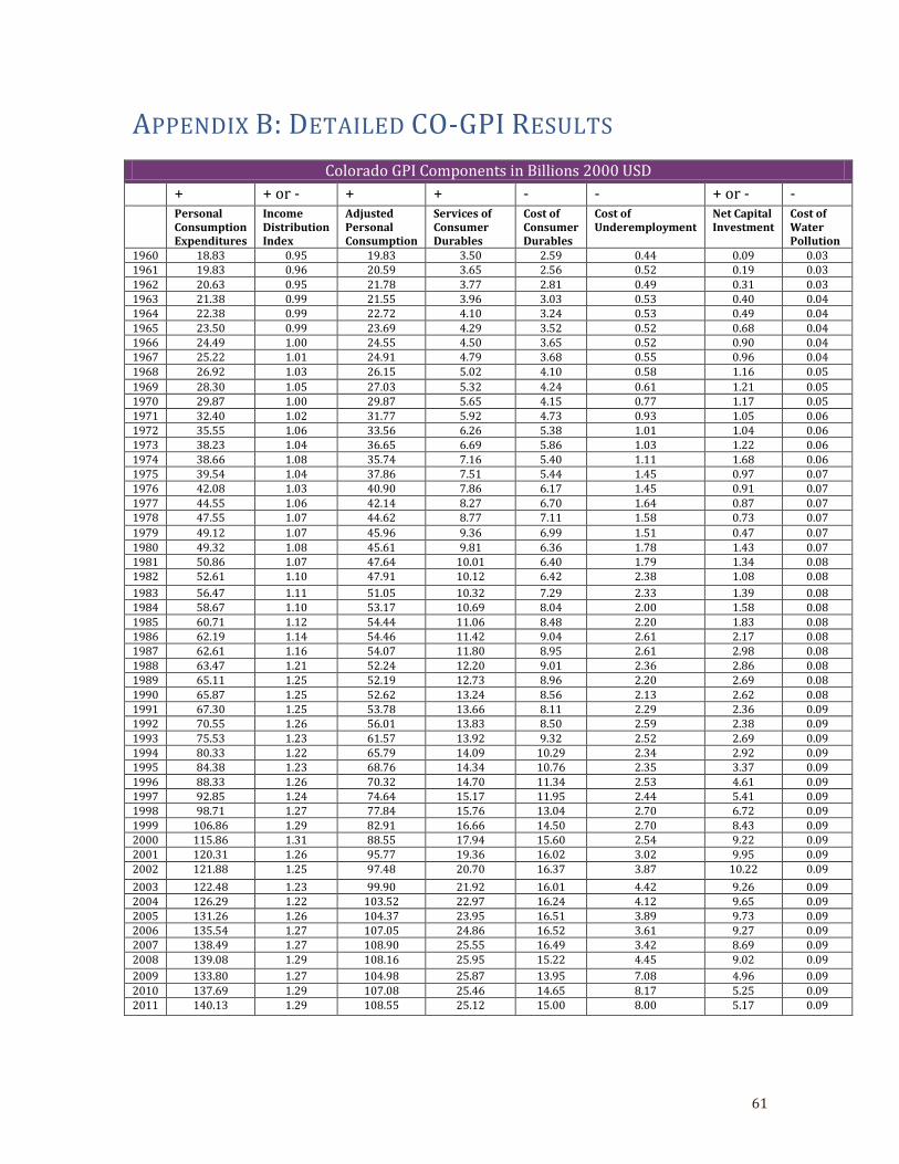
61

APPENDIX B: DETAILED CO-GPI RESULTS

Colorado GPI Components in Billions 2000 USD

+ + or - + + - - + or - - Personal

Consumption Expenditures

Income Distribution Index

Adjusted Personal Consumption

Services of Consumer Durables

Cost of Consumer Durables

Cost of Underemployment

Net Capital Investment

Cost of Water Pollution

1960 18.83 0.95 19.83 3.50 2.59 0.44 0.09 0.03 1961 19.83 0.96 20.59 3.65 2.56 0.52 0.19 0.03 1962 20.63 0.95 21.78 3.77 2.81 0.49 0.31 0.03 1963 21.38 0.99 21.55 3.96 3.03 0.53 0.40 0.04 1964 22.38 0.99 22.72 4.10 3.24 0.53 0.49 0.04 1965 23.50 0.99 23.69 4.29 3.52 0.52 0.68 0.04 1966 24.49 1.00 24.55 4.50 3.65 0.52 0.90 0.04 1967 25.22 1.01 24.91 4.79 3.68 0.55 0.96 0.04 1968 26.92 1.03 26.15 5.02 4.10 0.58 1.16 0.05

1969 28.30 1.05 27.03 5.32 4.24 0.61 1.21 0.05 1970 29.87 1.00 29.87 5.65 4.15 0.77 1.17 0.05 1971 32.40 1.02 31.77 5.92 4.73 0.93 1.05 0.06 1972 35.55 1.06 33.56 6.26 5.38 1.01 1.04 0.06 1973 38.23 1.04 36.65 6.69 5.86 1.03 1.22 0.06 1974 38.66 1.08 35.74 7.16 5.40 1.11 1.68 0.06 1975 39.54 1.04 37.86 7.51 5.44 1.45 0.97 0.07 1976 42.08 1.03 40.90 7.86 6.17 1.45 0.91 0.07 1977 44.55 1.06 42.14 8.27 6.70 1.64 0.87 0.07 1978 47.55 1.07 44.62 8.77 7.11 1.58 0.73 0.07

1979 49.12 1.07 45.96 9.36 6.99 1.51 0.47 0.07 1980 49.32 1.08 45.61 9.81 6.36 1.78 1.43 0.07 1981 50.86 1.07 47.64 10.01 6.40 1.79 1.34 0.08 1982 52.61 1.10 47.91 10.12 6.42 2.38 1.08 0.08

1983 56.47 1.11 51.05 10.32 7.29 2.33 1.39 0.08 1984 58.67 1.10 53.17 10.69 8.04 2.00 1.58 0.08 1985 60.71 1.12 54.44 11.06 8.48 2.20 1.83 0.08 1986 62.19 1.14 54.46 11.42 9.04 2.61 2.17 0.08 1987 62.61 1.16 54.07 11.80 8.95 2.61 2.98 0.08 1988 63.47 1.21 52.24 12.20 9.01 2.36 2.86 0.08 1989 65.11 1.25 52.19 12.73 8.96 2.20 2.69 0.08 1990 65.87 1.25 52.62 13.24 8.56 2.13 2.62 0.08 1991 67.30 1.25 53.78 13.66 8.11 2.29 2.36 0.09 1992 70.55 1.26 56.01 13.83 8.50 2.59 2.38 0.09 1993 75.53 1.23 61.57 13.92 9.32 2.52 2.69 0.09 1994 80.33 1.22 65.79 14.09 10.29 2.34 2.92 0.09 1995 84.38 1.23 68.76 14.34 10.76 2.35 3.37 0.09 1996 88.33 1.26 70.32 14.70 11.34 2.53 4.61 0.09 1997 92.85 1.24 74.64 15.17 11.95 2.44 5.41 0.09 1998 98.71 1.27 77.84 15.76 13.04 2.70 6.72 0.09 1999 106.86 1.29 82.91 16.66 14.50 2.70 8.43 0.09 2000 115.86 1.31 88.55 17.94 15.60 2.54 9.22 0.09 2001 120.31 1.26 95.77 19.36 16.02 3.02 9.95 0.09 2002 121.88 1.25 97.48 20.70 16.37 3.87 10.22 0.09

2003 122.48 1.23 99.90 21.92 16.01 4.42 9.26 0.09 2004 126.29 1.22 103.52 22.97 16.24 4.12 9.65 0.09 2005 131.26 1.26 104.37 23.95 16.51 3.89 9.73 0.09 2006 135.54 1.27 107.05 24.86 16.52 3.61 9.27 0.09 2007 138.49 1.27 108.90 25.55 16.49 3.42 8.69 0.09 2008 139.08 1.29 108.16 25.95 15.22 4.45 9.02 0.09

2009 133.80 1.27 104.98 25.87 13.95 7.08 4.96 0.09 2010 137.69 1.29 107.08 25.46 14.65 8.17 5.25 0.09 2011 140.13 1.29 108.55 25.12 15.00 8.00 5.17 0.09

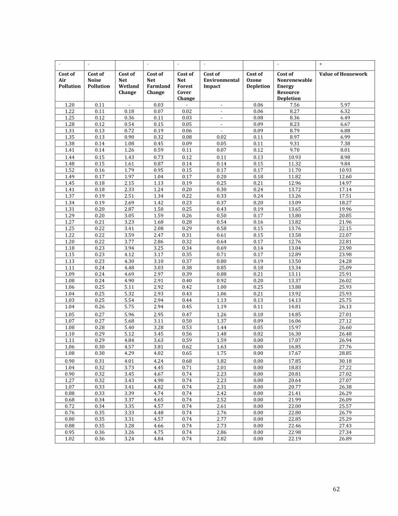
62

- - - - - - +

Cost of Air Pollution

Cost of Noise Pollution

Cost of Net Wetland Change

Cost of Net Farmland Change

Cost of Net Forest Cover Change

Cost of Environmental Impact

Cost of Ozone Depletion

Cost of Nonrenewable Energy Resource Depletion

Value of Housework

1.20 0.11 - 0.03 - - 0.06 7.56 5.97 1.22 0.11 0.18 0.07 0.02 - 0.06 8.27 6.32 1.25 0.12 0.36 0.11 0.03 - 0.08 8.36 6.49 1.28 0.12 0.54 0.15 0.05 - 0.09 8.23 6.67 1.31 0.13 0.72 0.19 0.06 - 0.09 8.79 6.88 1.35 0.13 0.90 0.32 0.08 0.02 0.11 8.97 6.99 1.38 0.14 1.08 0.45 0.09 0.05 0.11 9.31 7.38 1.41 0.14 1.26 0.59 0.11 0.07 0.12 9.70 8.01

1.44 0.15 1.43 0.73 0.12 0.11 0.13 10.93 8.98 1.48 0.15 1.61 0.87 0.14 0.14 0.15 11.32 9.84 1.52 0.16 1.79 0.95 0.15 0.17 0.17 11.70 10.93 1.49 0.17 1.97 1.04 0.17 0.20 0.18 11.82 12.60 1.45 0.18 2.15 1.13 0.19 0.25 0.21 12.96 14.97 1.41 0.18 2.33 1.24 0.20 0.30 0.24 13.72 17.14 1.37 0.19 2.51 1.34 0.22 0.33 0.24 13.26 17.51

1.34 0.19 2.69 1.42 0.23 0.37 0.20 13.09 18.27 1.31 0.20 2.87 1.50 0.25 0.43 0.19 13.65 19.96 1.29 0.20 3.05 1.59 0.26 0.50 0.17 13.80 20.85 1.27 0.21 3.23 1.68 0.28 0.54 0.16 13.82 21.96 1.25 0.22 3.41 2.08 0.29 0.58 0.15 13.76 22.15

1.22 0.22 3.59 2.47 0.31 0.61 0.15 13.58 22.07 1.20 0.22 3.77 2.86 0.32 0.64 0.17 12.76 22.81 1.18 0.23 3.94 3.25 0.34 0.69 0.14 13.04 23.90 1.15 0.23 4.12 3.17 0.35 0.71 0.17 12.89 23.98

1.13 0.23 4.30 3.10 0.37 0.80 0.19 13.50 24.28 1.11 0.24 4.48 3.03 0.38 0.85 0.18 13.34 25.09 1.09 0.24 4.69 2.97 0.39 0.88 0.21 13.11 25.91 1.08 0.24 4.90 2.91 0.40 0.92 0.20 13.37 26.02 1.06 0.25 5.11 2.92 0.42 1.00 0.25 13.88 25.93

1.04 0.25 5.32 2.93 0.43 1.06 0.21 13.92 25.93 1.03 0.25 5.54 2.94 0.44 1.13 0.13 14.13 25.75 1.04 0.26 5.75 2.94 0.45 1.19 0.11 14.81 26.13

1.05 0.27 5.96 2.95 0.47 1.26 0.10 14.85 27.01 1.07 0.27 5.68 3.11 0.50 1.37 0.09 16.06 27.12 1.08 0.28 5.40 3.28 0.53 1.44 0.05 15.97 26.60 1.10 0.29 5.12 3.45 0.56 1.48 0.02 16.30 26.48 1.11 0.29 4.84 3.63 0.59 1.59 0.00 17.07 26.94 1.06 0.30 4.57 3.81 0.62 1.63 0.00 16.85 27.76 1.08 0.30 4.29 4.02 0.65 1.75 0.00 17.67 28.85

0.90 0.31 4.01 4.24 0.68 1.82 0.00 17.85 30.18 1.04 0.32 3.73 4.45 0.71 2.01 0.00 18.83 27.22 0.90 0.32 3.45 4.67 0.74 2.23 0.00 20.81 27.02 1.27 0.32 3.43 4.90 0.74 2.23 0.00 20.64 27.07 1.07 0.33 3.41 4.82 0.74 2.31 0.00 20.77 26.38 0.88 0.33 3.39 4.74 0.74 2.42 0.00 21.41 26.29 0.68 0.34 3.37 4.65 0.74 2.52 0.00 21.99 26.09 0.72 0.34 3.35 4.57 0.74 2.61 0.00 22.00 25.57 0.76 0.35 3.33 4.48 0.74 2.76 0.00 22.80 26.79 0.80 0.35 3.31 4.57 0.74 2.77 0.00 22.85 25.29

0.88 0.35 3.28 4.66 0.74 2.73 0.00 22.46 27.43 0.95 0.36 3.26 4.75 0.74 2.86 0.00 22.98 27.34 1.02 0.36 3.24 4.84 0.74 2.82 0.00 22.19 26.89

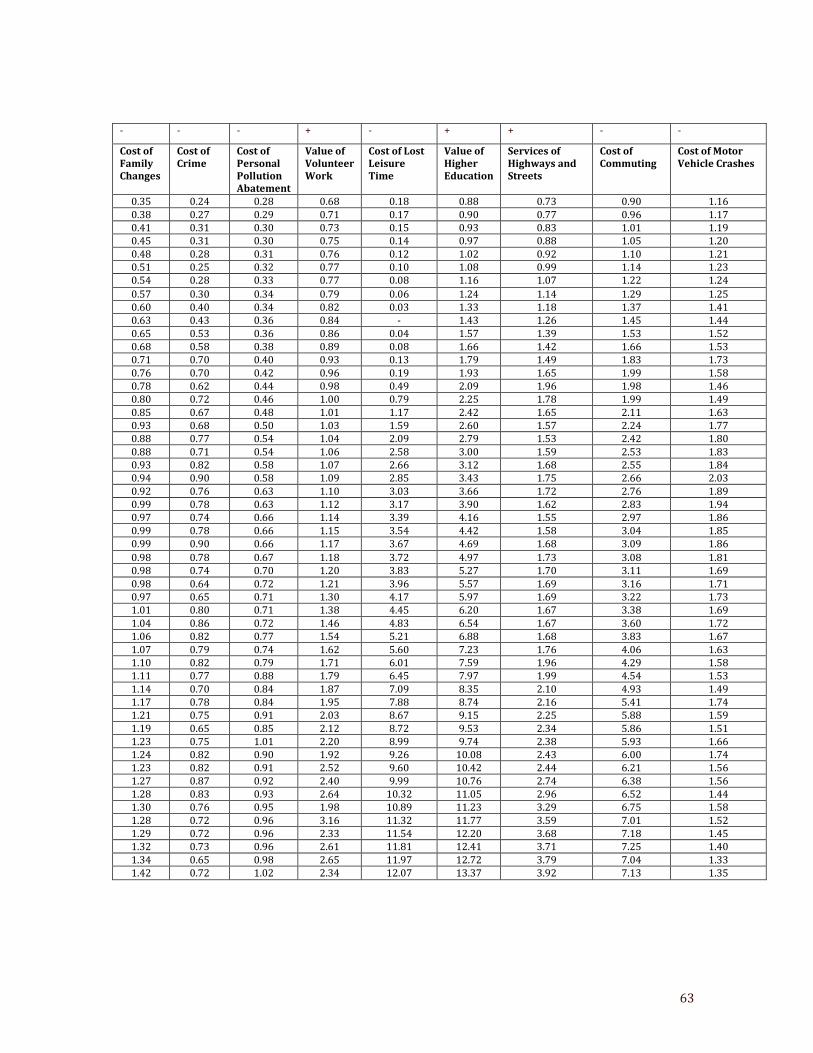
63

- - - + - + + - -

Cost of Family Changes

Cost of Crime

Cost of Personal Pollution Abatement

Value of Volunteer Work

Cost of Lost Leisure Time

Value of Higher Education

Services of Highways and Streets

Cost of Commuting

Cost of Motor Vehicle Crashes

0.35 0.24 0.28 0.68 0.18 0.88 0.73 0.90 1.16 0.38 0.27 0.29 0.71 0.17 0.90 0.77 0.96 1.17 0.41 0.31 0.30 0.73 0.15 0.93 0.83 1.01 1.19 0.45 0.31 0.30 0.75 0.14 0.97 0.88 1.05 1.20 0.48 0.28 0.31 0.76 0.12 1.02 0.92 1.10 1.21 0.51 0.25 0.32 0.77 0.10 1.08 0.99 1.14 1.23 0.54 0.28 0.33 0.77 0.08 1.16 1.07 1.22 1.24

0.57 0.30 0.34 0.79 0.06 1.24 1.14 1.29 1.25 0.60 0.40 0.34 0.82 0.03 1.33 1.18 1.37 1.41 0.63 0.43 0.36 0.84 - 1.43 1.26 1.45 1.44 0.65 0.53 0.36 0.86 0.04 1.57 1.39 1.53 1.52 0.68 0.58 0.38 0.89 0.08 1.66 1.42 1.66 1.53 0.71 0.70 0.40 0.93 0.13 1.79 1.49 1.83 1.73 0.76 0.70 0.42 0.96 0.19 1.93 1.65 1.99 1.58 0.78 0.62 0.44 0.98 0.49 2.09 1.96 1.98 1.46 0.80 0.72 0.46 1.00 0.79 2.25 1.78 1.99 1.49 0.85 0.67 0.48 1.01 1.17 2.42 1.65 2.11 1.63 0.93 0.68 0.50 1.03 1.59 2.60 1.57 2.24 1.77 0.88 0.77 0.54 1.04 2.09 2.79 1.53 2.42 1.80 0.88 0.71 0.54 1.06 2.58 3.00 1.59 2.53 1.83 0.93 0.82 0.58 1.07 2.66 3.12 1.68 2.55 1.84 0.94 0.90 0.58 1.09 2.85 3.43 1.75 2.66 2.03 0.92 0.76 0.63 1.10 3.03 3.66 1.72 2.76 1.89 0.99 0.78 0.63 1.12 3.17 3.90 1.62 2.83 1.94 0.97 0.74 0.66 1.14 3.39 4.16 1.55 2.97 1.86 0.99 0.78 0.66 1.15 3.54 4.42 1.58 3.04 1.85 0.99 0.90 0.66 1.17 3.67 4.69 1.68 3.09 1.86

0.98 0.78 0.67 1.18 3.72 4.97 1.73 3.08 1.81 0.98 0.74 0.70 1.20 3.83 5.27 1.70 3.11 1.69 0.98 0.64 0.72 1.21 3.96 5.57 1.69 3.16 1.71 0.97 0.65 0.71 1.30 4.17 5.97 1.69 3.22 1.73 1.01 0.80 0.71 1.38 4.45 6.20 1.67 3.38 1.69 1.04 0.86 0.72 1.46 4.83 6.54 1.67 3.60 1.72 1.06 0.82 0.77 1.54 5.21 6.88 1.68 3.83 1.67 1.07 0.79 0.74 1.62 5.60 7.23 1.76 4.06 1.63 1.10 0.82 0.79 1.71 6.01 7.59 1.96 4.29 1.58 1.11 0.77 0.88 1.79 6.45 7.97 1.99 4.54 1.53 1.14 0.70 0.84 1.87 7.09 8.35 2.10 4.93 1.49 1.17 0.78 0.84 1.95 7.88 8.74 2.16 5.41 1.74 1.21 0.75 0.91 2.03 8.67 9.15 2.25 5.88 1.59 1.19 0.65 0.85 2.12 8.72 9.53 2.34 5.86 1.51 1.23 0.75 1.01 2.20 8.99 9.74 2.38 5.93 1.66 1.24 0.82 0.90 1.92 9.26 10.08 2.43 6.00 1.74 1.23 0.82 0.91 2.52 9.60 10.42 2.44 6.21 1.56 1.27 0.87 0.92 2.40 9.99 10.76 2.74 6.38 1.56 1.28 0.83 0.93 2.64 10.32 11.05 2.96 6.52 1.44 1.30 0.76 0.95 1.98 10.89 11.23 3.29 6.75 1.58 1.28 0.72 0.96 3.16 11.32 11.77 3.59 7.01 1.52 1.29 0.72 0.96 2.33 11.54 12.20 3.68 7.18 1.45 1.32 0.73 0.96 2.61 11.81 12.41 3.71 7.25 1.40 1.34 0.65 0.98 2.65 11.97 12.72 3.79 7.04 1.33 1.42 0.72 1.02 2.34 12.07 13.37 3.92 7.13 1.35