PR

IFY

SG

OL

BA

NG

OR

/ B

AN

GO

R U

NIV

ER

SIT

Y

Combining univariate approaches for ensemble change detection inmultivariate dataFaithfull, William; Rodriguez, Juan; Kuncheva, Ludmila

Information Fusion

Published: 01/01/2019

Peer reviewed version

Cyswllt i'r cyhoeddiad / Link to publication

Dyfyniad o'r fersiwn a gyhoeddwyd / Citation for published version (APA):Faithfull, W., Rodriguez, J., & Kuncheva, L. (2019). Combining univariate approaches forensemble change detection in multivariate data. Information Fusion, 45, 202-214.

Hawliau Cyffredinol / General rightsCopyright and moral rights for the publications made accessible in the public portal are retained by the authors and/orother copyright owners and it is a condition of accessing publications that users recognise and abide by the legalrequirements associated with these rights.

• Users may download and print one copy of any publication from the public portal for the purpose of privatestudy or research. • You may not further distribute the material or use it for any profit-making activity or commercial gain • You may freely distribute the URL identifying the publication in the public portal ?

Take down policyIf you believe that this document breaches copyright please contact us providing details, and we will remove access tothe work immediately and investigate your claim.

13. May. 2020

Combining Univariate Approaches forEnsemble Change Detection in Multivariate Data

William J. Faithfulla,∗, Juan J. Rodrıguezb, Ludmila I. Kunchevaa

aSchool of Computer Science, Bangor University, Dean Street, Bangor, Gwynedd, Wales LL57 1UT, UKbEscuela Politecnica Superior, University of Burgos, Avda. de Cantabria s/n, 09006 Burgos, Spain

Abstract

Detecting change in multivariate data is a challenging problem, especially when class labels are not available. There is a large body ofresearch on univariate change detection, notably in control charts developed originally for engineering applications. We evaluate univariatechange detection approaches —including those in the MOA framework — built into ensembles where each member observes a featurein the input space of an unsupervised change detection problem. We present a comparison between the ensemble combinations and threeestablished ’pure’ multivariate approaches over 96 data sets, and a case study on the KDD Cup 1999 network intrusion detection dataset. Wefound that ensemble combination of univariate methods consistently outperformed multivariate methods on the four experimental metrics.

1. Introduction

Change detection is, at its simplest, the task of identifying datapoints that differ from those seen before. It is often deployed ina supervised or unsupervised context: monitoring the error rateof a learning algorithm which processes the target data, or directlymonitoring the target data. In the second context, we do not haveclass labels with which to estimate an error rate. Unsupervisedchange detection in a single variable is the univariate case of theproblem and has been extensively studied over more than half acentury, yielding widely used approaches such as control charts,and specifically, the cumulative sum chart (CUSUM) [1, 2]. Thereare a variety of univariate methods across the literature from severalfields. Basseville and Nikiforov [3] published a monograph ondetectors of abrupt change in 1993. There are extensive methodreviews in the overlapping field of novelty detection, by Markouand Singh [4] and Pimentel et al. [5], and in outlier detection byBen-Gal [6]. There are many approaches from the classificationliterature intended to monitor the error-rate of the incoming dataand adapt a deployed classifier accordingly. The MOA (MassiveOnline Analysis) framework [7, 8] is a popular open source toolfor data stream mining, providing a number of approaches forunivariate change detection, all of which we evaluate in this work.

We take inspiration from our previous study [9] where we useclassifier ensembles to detect concept change in unlabelled multi-variate data. We propose an ensemble of univariate detectors (whichcould be called a ‘subspace ensemble’) as a means of adaptingestablished univariate change detection methods to multivariateproblems. Our hypothesis is that such an ensemble should be com-petitive or better than ’pure’ unsupervised multivariate approaches.We contribute the following: 1. An evaluation of which established

∗Corresponding AuthorEmail addresses:

w.faithfull@bangor.ac.uk (William J. Faithfull), jjrodriguez@ubu.es

(Juan J. Rodrıguez), l.i.kuncheva@bangor.ac.uk (Ludmila I. Kuncheva)

univariate change detection methods are well suited to subspaceensemble combination over 96 common datasets. 2. Whether sub-space ensembles outperform three established multivariate changedetection methods, especially in high dimensions. 3. A reproduciblereinterpretation of the widely used KDD Cup 1999 [10] networkintrusion detection dataset as a change detection problem.

When generalising unsupervised change detection to multiple di-mensions, the challenges proliferate – in how many features shouldwe expect to see change before signalling? Can we reasonablyassume that all features and examples are independent? Multivariateapproaches often assume that each example is drawn from amultivariate process [11, 12, 13, 14]. Thus, we need not assume thatthe features are independent. Multivariate change detection attemptsto model a multivariate process by means of a function to evaluatethe fit of new data (an example or a batch) to that model. Someworks monitor components independently (Tartatovsky et al. [15]and Evangelista et al. [16]), meaning that the approach is unable torespond to changes in the correlation of the components. Whether ornot this is a disadvantage, depends upon the context of the change.

Change may have a different definition for different problems.For example, if we wish to be alerted when the value of a stock isfalling, a sudden rise might be irrelevant. If using a control chart withupper and lower limits, only monitoring the lower limit might consid-erably lower the false alarm rate. If the problem is well known thena heuristic can be applied, but if that is the case, there is most likelytraining data available for a supervised approach. Unsupervised ap-proaches must be robust in the face of unknown context. The changewe wish to detect could be abrupt or gradual. It could be a singlechange or repeating concepts. When we move into multiple dimen-sions, there is even more scope for contextual properties to stretchour assumptions. Change could manifest itself in a single feature, allfeatures, or any number of features in-between. From the novelty de-tection literature, Evangelista et al. [16] conclude that unsupervisedlearning in subspaces of the data will typically outperform unsuper-vised learning that considers the data as a whole. In the course of

Preprint submitted to Information Fusion February 19, 2018

this work, we investigate whether this assertion is reproducible.The dimensionality of the input data presents a potential

challenge. Allipi et. al [17] analyse the effect of an increasingdata dimension d on change detectability for log-likelihood basedmultivariate change detection methods. They demonstrate thatin the case of Gaussian random variables, change detectabilityis upper-bounded by a function that decays as 1

d . Importantly,the loss in detectability arises from a linear relationship betweenthe variance of the log-likelihood ratio and the data dimension.Evangelista et al. [16] propose that subspace ensembles are alsoa means to address the curse of dimensionality.

Multivariate detectors treat features as components of an underly-ing multivariate distribution [11]. We will term such detectors ‘pure’multivariate detectors. For pure detectors to work well, the datadimensionality d should not be high, as Allipi et al. argued, and thedata coming from the same concept should be available in an i.i.dsequence. This is rarely the case in practice. For example, Tarta-tovsky et al. [15] observe that the assumption that all examples arei.i.d is very restrictive in the domain of network intrusion detection.

The remainder of the paper is organised as follows. Section 2covers the background and related work for this problem. Section3 details the methods used, explains our combination mechanism,and overviews the experimental protocol. Our results are presentedin Section 4, and our conclusions follow in Section 5.

2. Background & Related Work

Learning methods are frequently deployed in non-stationaryenvironments, where the concepts may change unpredictably overtime. Where class labels are immediately or eventually available,change detection methods can be required to monitor only aunivariate error stream from a learner. When a change is detectedin the error stream, we can retrain or adapt the model as required.However, when labels are not available, then we cannot use theerror rate as a performance indicator. In this instance, a fullyunsupervised approach must be taken.

Surveys by Gama et al. [18] and Ditzler et al. [19] discuss thedistinction between real and virtual concept drift. Real conceptdrift is a change in the class conditional probabilities, i.e. theoptimal decision boundary. Virtual concept drift refers to a changein the prior probabilities, or distribution of the data. Since inan unsupervised setting, we have no class labels to identify realconcept drift, this work would conform to the latter definition. Thisparticular problem formulation is closely related to the assumptionsof statistical process control, novelty detection, and outlier detection,for which applications are usually unsupervised, and methods areexpected to be applied directly to the domain data.

Most methods for multivariate change detection require two com-ponents: a means to estimate the distribution of the incoming data,and a test to evaluate whether new data points fit that model. Estima-tion of the streaming data distribution is commonly done by eitherclustering, or multivariate distribution modelling. Gaussian MixtureModels (GMM) are a popular parametric means to model a multi-variate process for novelty detection, as in Zorriassatine et al. [12].Tarassenko et al. [20] and Song et al. [21] use nonparametric Parzenwindows (kernel density estimation) to approximate a model against

which new data is compared. Dasu et al. [22] construct kdq treesto a similar effect. Krempl et al [23] track the trajectories of onlineclustering, while Gaber and Yu [24] use the deviation in the cluster-ing results to identify evolution of the data stream. Kuncheva [11]applies k means clustering to the input data and uses the clusterpopulations to approximate the distribution of the data.

Multivariate statistical tests for comparing distributions such, asHotelling’s t-squared test [25] need to be adapted into the sequentialform over time windows of the data [11]. Bespoke statisticscontinue to be developed for this purpose [13, 14]. Kuncheva [11]introduces a family of log-likelihood ratio detectors which use twotime-windows of multivariate data to compute the probability thatboth are drawn from the same distribution. The observation thatlog-likelihood based detectors effectively reduce the input spaceto a univariate statistic can be further exploited, by monitoring thatratio with existing univariate methods [26].

Ensemble methods for monitoring evolving data streams is agrowing area of interest within the change detection literature.There are recent surveys on the subject by Krawczyk et al. [27] andGomes et al. [28]. The former observe that there has been relativelylittle research on the combination of drift detection methods. Thepublications that they review in this area [29, 30] deal with thecombination of detectors over univariate input data, in contrast to ourown formulation. The latter work introduces a taxonomy for datastream ensemble learning methods, and demonstrates the diversityof available methods for ensemble combination. Du et al. [31]utilise an ensemble of change detectors in a supervised approach fora univariate error stream. Alippi et al. [32] introduce hierarchicalchange detection tests (HCDTs) combining a fast, sequential changedetector with a slower, optionally-invoked offline change detector.

In the classification literature, ensemble change detectioncommonly refers to using these techniques to monitor the accuracyof classifiers in an ensemble, in order to decide when to retrainor replace a classifier [33, 34, 35, 36]. Many of these establishedunivariate methods for change detection are geared towards thesupervised scenario which offers a discrete error stream [37, 38].The Streaming Ensemble Algorithm (SEA) [39] was one of the firstof many ensemble approaches for streaming supervised learningproblems. However, instead of relying on a change detection,SEA creates an adaptive classifier which is robust to concept drift.Evangelista et al. [16] use a subspace ensemble of one-class SupportVector Machine classifiers in the context of novelty detection. Theinput space is divided into 3 random subspaces, each monitored bya single ensemble member. Kuncheva [9] uses classifier ensemblesto directly detect concept change in unlabeled data, sharing thesame problem formulation as this work.

3. Change detection methods

The methods we evaluated are detailed in Tables 1 and 2. Wechose to evaluate all the univariate detectors offered by MOA [7, 8],an open source project for data stream analysis. Our experiment per-forms an unsupervised evaluation of all reference implementationsof the ChangeDetector interface in the MOA package

moa.classifiers.core.driftdetection 1

1https://github.com/Waikato/moa/tree/master/moa/src/main/

2

Table 1: Methods for change detection in univariate data

Method References CategorySEED [40] Monitoring DistributionsADWIN [41, 8] Monitoring DistributionsSEQ1 [42] Monitoring DistributionsPage-Hinkley [1, 8] Sequential AnalysisCUSUM1 [1] Sequential AnalysisCUSUM2 [8] Sequential AnalysisGEOMA [43, 44] Control ChartHDDMA [36] Control ChartEDDM [38, 8] Control ChartDDM [37, 8] Control ChartEWMA [43, 8, 44] Control ChartHDDMW [36] Control Chart

Table 2: Methods for change detection in multivariate data

Method References CategorySPLL [11] Monitoring Distributions

Log-likelihood KL [11] Monitoring DistributionsLog-likelihood Hotelling [11] Monitoring Distributions

The interface contract implies the following basic methods toprovide an input and subsequently check if change was detected:

public void input(double inputValue);

public boolean getChange();

All the univariate detectors are provided by MOA except CUSUM1,which is a CUSUM chart with upper and lower limits which wasimplemented in Java, and integrated into the experiment to serve asa baseline. We arrive at a final figure of 88 detectors, 3 of which arethe multivariate approaches listed in Table 2, and the remaining 85are ensembles of the univariate approaches with varying thresholds.The experimental details will be given in subsection 3.2. A full list ofthe 96 datasets and their characteristics can be found in Table 4. Ourmetrics for evaluation and our experimental protocol are addressed insubsection 3.3. Finally, we discuss the case study in subsection 3.4.

3.1. Overview of the methodsThe univariate detectors are listed in Table 1, with their

accompanying publications. We categorise the methods based onthe change detection taxonomy presented in Gama et. al [18]. Whatfollows is a high-level overview of the theory behind each categoryof methods along with an abridged description of each detector.More details for each detector can be found in the accompanyingpublications in Table 1. The source code for each detector isavailable for inspection in the MOA repository.

3.1.1. Sequential AnalysisSequential analysis methods have much in common with the

Sequential Probability Ratio Test (SPRT) [2]. Consider a sequenceof examples X = [x1, ..., xN]. The null hypothesis H0 is that Xis generated from a given distribution p0(x), and the alternative

java/moa/classifiers/core/driftdetection

hypothesis H1 is that X is generated from another (known)distribution p1(x). The logarithm of the likelihood ratio for the twodistributions is calculated as

ΛN =

N∑i=1

logp1(xi)p0(xi)

Two thresholds, α and β are defined depending on the target errorrates. If ΛN <α, H0 is accepted, else if ΛN >β, H1 is accepted. Inthe case where α<=ΛN<=β, the decision is postponed, the next ex-ample in the stream, xN+1, is added to the set, and ΛN+1 is calculatedand compared with the thresholds. Cumulative sum (CUSUM) [1]is a sequential analysis technique based on the same principle. Thetest is widely used for detecting significant change in the mean ofinput data. Starting with an upper cumulative sum statistic g40 =0,CUSUM updates g4 for each subsequent example as

g4i =max(0,g4i−1+(xi−δ))

where δ is the magnitude of acceptable change. Change is signalledwhen g4i > λ, where λ is a fixed threshold. If we wish to detectboth positive and negative shifts in the mean, we can also computeand threshold the lower sum as

g5i =min(0,g5i−1−(xi−δ))

The Page-Hinkley test [1] is derived from CUSUM, andadapted to detect an abrupt change in the average of a Gaussianprocess [18, 45].

3.1.2. Control ChartsControl charts2 are a category of methods that are based upon

Statistical Process Control (SPC). In SPC, the modus operandiis to consider the problem as a known statistical process, andmonitor its evolution. Assume that we monitor classification error.This error can be interpreted as a Bernoulli random variable withprobability of “success” (where error occurs) p. The probabilityis unknown at the start of the monitoring, and is re-estimated withevery new example as the proportion of errors encountered thus far.At example i, we have a binomial random variable with estimatedprobability pi and standard deviation σi =

√pi(1−pi)/i. One way

to use this estimate is described below [37, 18]:

1. Denote the (binary) streaming examples as x1,x2,.... To keepa running score of the minimum p, start with estimate pmin =1,and σmin =0. Initialise the stream counter i←1.

2. Observe xi. Calculate pi and σi. For an error and a standarddeviation (pi, σi) at example xi, the method follows a setof rules to place itself into one of three possible states: incontrol, warning, and out of control. Under the commonlyused confidence levels of 95% and 99%, the rules are:

2A number of the control chart methods in MOA are intended for supervisedpredictive error monitoring rather than continuous data., however they acceptcontinuous data by virtue of the ChangeDetector interface. While theirassumptions are violated by the unsupervised experiment, we include their resultsfor demonstrative purposes as MOA does not make a distinction. The Page-Hinkleydetector might be expected to perform better on a prequential error stream [46], butretains valid assumptions for unsupervised features.

3

• If pi +σi < pmin +2σmin, then the process is deemed tobe in control.

• If pi +σi ≥ pmin +3σmin, then the process is deemed tobe out of control.

• If pmin + 2σmin ≤ pi +σi < pmin + 3σmin, then this isconsidered to be the warning state.

3. If pi + σi < pmin + σmin, re-assign the minimum values:pmin← pi and σmin←σi.

4. i← i+1. Continue from 2.

The geometric moving average chart (GEOMMA), introducedby Roberts [44], assigns weights to each observation such that theweight of older observations decreases in geometric progression.This biases the method towards newer observations, improving theadaptability. Exponentially Weighted Moving Average (EWMA)charts are a progression of this approach such that the rate of weightdecay is continuous and can be tuned.

The EWMA charts used by Ross et al. [43] expect the initialdistribution to have known parameters, which is a restrictiveassumption in the area of change detection. To address thislimitation, the initial distribution is approximated in advancethrough regression of the distributional parameters to achieve adesired Average Running Length (ARL).

Drift Detection Method (DDM) [37] is designed to monitor clas-sification error using a control chart construction. It assumes that theerror rate will decrease while the underlying distribution is stationary.

Similarly, the Early Drift Detection Method (EDDM) [38] isan extension of DDM which takes into account the time distancebetween errors as opposed to considering only the magnitudeof the difference, which is aimed at improving the performanceof the detector on gradual change. HDDMA and HDDMW areextensions which remove assumptions relating the to probabilitydensity functions of the error of the learner. Instead, they assumethat the input is an independent and bounded random variable, anduse Hoeffding’s inequality to compute the bounds [36].

3.1.3. Monitoring two distributionsThe methods in this category monitor the distributions of two

windows of data. The basic construction involves a referencewindow composed of old data, and a detection window composedof new data. This can be achieved with a static reference windowand a sliding detection window, or a sliding pair of windowsover consecutive observations. The old and new windows can becompared with statistical tests, with the null hypothesis being thatboth windows are drawn from the same distribution.

For fixed-sized windows, their sizes need to be decided apriori, which poses a problem. A small-sized window discardsold examples swiftly, best representing the current state, but it alsomakes the method vulnerable to outliers. Conversely, a large-sizedwindow provides more stable estimates of the probabilities and othervariables of interest, but takes longer to pick up a change. In orderto address this selection problem, there are a number of approachesfor growing and shrinking sliding windows on the fly [41, 47, 48].

A widely-used approach of this type is Adaptive Windowing(ADWIN) by Bifet and Gavalda [41]. It keeps a variable-length win-dow of recently seen examples, and a fixed-size reference window.

For the variable size window, ADWIN keeps the longest possiblewindow within which there has been no statistically significantchange. In its formulation as a change detector, change is signalledwhen the difference of the averages of the windows exceeds acomputed threshold. When this threshold is reached, the referencewindow is emptied, and replaced by the variable length window,which is then regrown from subsequent observations. The SEQ1algorithm [42] is an evolution of the ADWIN approach with a lowercomputational complexity. Cut-points are computed differently– where ADWIN makes multiple passes through the window tocompute candidate cut-points, SEQ1 only examines the boundarybetween the latest and previous batch of elements. Secondly, themeans of data segments are estimated through random samplinginstead of exponential histograms. Finally, the authors employthe Bernstein bound instead of the Hoeffding bound to establishwhether two sub-windows are drawn from the same populationbecause the Hoeffding bound was deemed to be overly conservative.

In the SEED algorithm by Huang et al. [40], the data comesin blocks of a fixed size, so the candidate change points are theblock’s starting and ending points. Adjacent blocks are examinedand grouped together if they are deemed sufficiently similar. Thisoperation, termed ‘block compression’, removes candidate changepoints which have a lower probability of being true change points.Pooling blocks together amounts to obtaining larger windows,which in turn, ensures more stable estimates of the probabilitiesof interest compared to estimates from the original blocks. Driftdetection is subsequently carried out by analysing possible splitsbetween the newly-formed blocks.

3.1.4. Multivariate change detectorsConsider a random vector x

x=[x1,x2,...,xn]T ∈Rn,

drawn from a continuous stream

xi,xi+1,...,xN...

We assume that x are drawn from a probability distribution p0(x)up to a certain point c in the stream, and from a different distributionthereafter. The objective is to find the change point c. We canestimate p0 from the incoming examples and compute the likelihoodL(x|p0) for subsequent examples. A successful detection algorithmwill be able to identify c by a decrease of the likelihood of theexamples arriving after c. To estimate and compare the likelihoodsbefore and after a candidate point, the data is partitioned into a pairof adjacent sliding time-windows of examples, W1 and W2.

The Hotelling detector uses the multivariate T2 test for equalmeans, and assumes equal covariance matrices of W1 and W2.Therefore, if the change of the distribution comes from change inthe variances or covariances in the multidimensional space of thedata, the test will be powerless.

As an alternative, we used a non-parametric change detectorbased on the Kullback-Leibler divergence (KL). To this end, the datain W1 is clustered using k-means into K clusters, C ={C1,...,CK}. Adiscrete distribution P is defined on C, where each cluster is givena probability equal to the proportion of examples it holds. Theexamples in W2 are labelled in the K clusters by the nearest cluster

4

1Features

2

n

Change Detector 1

Change Detector 2

...

Change Detector n

DecisionFusion

01

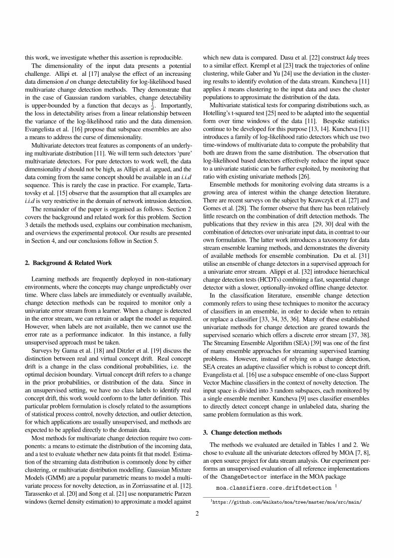
Figure 1: An illustration of the ensemble combination scheme. All change detectorsare of the same type, but each monitors a different feature.

centroid. The proportions of examples labelled in the respectivecluster define the distribution Q over C, this time derived fromthe data in W2. If the two distributions were identical, the KLdivergence will be close to 0, and if they are very different, it will beclose to 1. The success on this detector depends on a wise choice ofthe number of clusters K relative to the window sizes and the spacedimensionality n. A smaller number of clusters ensures that thereare enough points in each cluster to allow for reasonable estimates ofthe probability mass function. On the other hand, a larger number ofclusters allows for better fidelity in approximating the distributions.

Finally, we include in the experiment the Semi-Parametric Log-Likelihood detector (SPLL) [11] as a compromise between the para-metric detector (Hotelling) and non-parametric detector (KL). SPLL,like KL, applies k-means clustering to W1 into K clusters. However,rather than approximating a discrete distribution, the criterion func-tion of SPLL is derived assuming that we have fitted a Gaussian mix-ture with equal mixing proportion and common covariance matrixfor the K clusters. The first part of the statistic of the SPLL detectoris proportional to the mean of the squared Mahalanobis distancesbetween each example in W2 and its nearest cluster centroid. Thecalculation is repeated symmetrically by clustering first W2, and thenassigning labels to the examples in W1. This gives the second partof the SPLL statistic. These two parts are subsequently averaged.3

3.2. Ensemble combination of univariate detectorsIn order to evaluate univariate approaches on multivariate data,

we adopted an ensemble combination strategy whereby eachmember monitors a single feature of the input space. This approachis analogous to using a subspaces ensemble method with a subspacesize of 1, with as many subspaces and detectors as the dimensional-ity of the input space. Using subspaces with a size greater than 1, asin Evangelista et al. [16], would require combination of multivariateapproaches. Figure 1 shows an illustration of the ensemblecombination scheme. In this set of experiments, the decisions arecombined by a simple voting scheme with a variable threshold. Ournaming convention for a single ensemble is as follows:

DETECTOR - AGREEMENT THRESHOLD (1)

For example, ADWIN-30 refers to an ensemble of univariateADWIN detectors, which requires 30% agreement at any given

3MATLAB code is available athttps://github.com/LucyKuncheva/Change-detection

point to signal change. The multivariate detectors will simply bereferred to as, KL, SPLL and Hotelling, as they are not ensembles.4

Diversity is an important consideration when building anensemble, because it implies that the members will make differentmistakes [49, 50] and there have been several analyses of ensemblediversity in evolving data streams [51, 28]. However, unlike inthese works, our ensembles consist of identical detectors. Diversityis introduced through the differing input to each detector. On arelated note, there will be redundant features in the datasets, whichwill effect ensemble performance. Ideally this would be addressedthrough a feature extraction step, but such a measure is both difficultto generalise across datasets and outside the scope of this paper. Asour ensembles are created with identical members, no one type ofdetector can gain an advantage in the results due to drawing manyredundant features by chance.

3.3. Experimental protocolThe main experiment of this paper evaluates our multivariate

change detection methods across the 96 datasets in Table 4. Weevaluate the 3 multivariate detectors – SPLL, KL and Hotelling,an ensemble of these multivariate detectors, and 84 feature-wiseensembles of the univariate detectors with varying agreementthresholds, making a total of 88 detectors. A breakdown of themethods is presented in Table 3.

We note that when the thresholds in Table 3 are utilised onparticularly small ensembles, the lower thresholds will becomelogically equivalent. For example, in ensembles with fewer than 20members, the 5% and 1% thresholds will make the same decisions(20×0.5 = 1). Since 43.33% of the datasets have more than 20features, the difference in results between these lower thresholdswill depend upon the larger datasets.

All the methods were evaluated against three rates of change:Abrupt, Gradual 100 and Gradual 300, for which we recordedseparate sets of results. Algorithm 1 is a simplified pseudocoderepresentation of the experiment. For each leg of the experiment,each detector is evaluated 100 times for each dataset. On each ofthese runs, we choose a random subset of the classes, and take thissubset to represent distribution p0 (before the change). The subsetwith the remaining classes is taken to represent distribution p1 (afterthe change). Points are then sampled randomly, with replacement,from the p0 and p1 sets – 500 examples in the abrupt case, 600 and800 respectively in the gradual cases. Denote these samples by S 1and S 2, respectively. We add a small random value to each example,scaled by the standard deviation of the data, to avoid examples thatare exact replicas. In the abrupt case, S 1 and S 2 are concatenatedto create a 1000-example test sample with with i.i.d stream fromindex 1 to 500, coming from p0, followed by an abrupt changeat index 500 to another i.i.d. stream of examples coming from p1.To emulate gradual change over 100 examples, we take S 1 and S 2as before, but do not concatenate them. At index 500, we samplewith increasing frequency from S 2. The chance of an example

4The ensemble of multivariate detectors is a special case, because, unlike theensembles of univariate detectors, it consists of only three detectors. In this case,the number of members does not scale with the number of features. As such, thereis no benefit in having a scale of agreement thresholds when there are only ever3 ensemble members. We chose 50% as a simple majority out of 3.

5

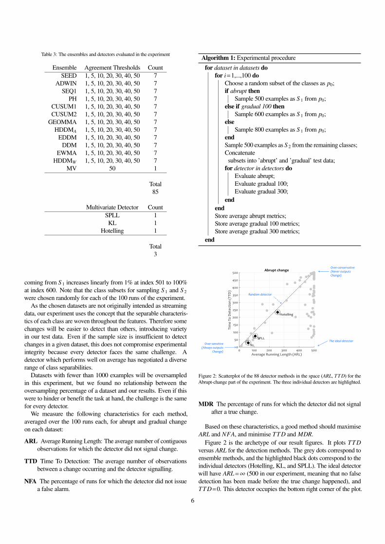
Table 3: The ensembles and detectors evaluated in the experiment

Ensemble Agreement Thresholds CountSEED 1, 5, 10, 20, 30, 40, 50 7

ADWIN 1, 5, 10, 20, 30, 40, 50 7SEQ1 1, 5, 10, 20, 30, 40, 50 7

PH 1, 5, 10, 20, 30, 40, 50 7CUSUM1 1, 5, 10, 20, 30, 40, 50 7CUSUM2 1, 5, 10, 20, 30, 40, 50 7

GEOMMA 1, 5, 10, 20, 30, 40, 50 7HDDMA 1, 5, 10, 20, 30, 40, 50 7

EDDM 1, 5, 10, 20, 30, 40, 50 7DDM 1, 5, 10, 20, 30, 40, 50 7

EWMA 1, 5, 10, 20, 30, 40, 50 7HDDMW 1, 5, 10, 20, 30, 40, 50 7

MV 50 1

Total85

Multivariate Detector CountSPLL 1KL 1

Hotelling 1

Total3

coming from S 1 increases linearly from 1% at index 501 to 100%at index 600. Note that the class subsets for sampling S 1 and S 2were chosen randomly for each of the 100 runs of the experiment.

As the chosen datasets are not originally intended as streamingdata, our experiment uses the concept that the separable characteris-tics of each class are woven throughout the features. Therefore somechanges will be easier to detect than others, introducing varietyin our test data. Even if the sample size is insufficient to detectchanges in a given dataset, this does not compromise experimentalintegrity because every detector faces the same challenge. Adetector which performs well on average has negotiated a diverserange of class separabilities.

Datasets with fewer than 1000 examples will be oversampledin this experiment, but we found no relationship between theoversampling percentage of a dataset and our results. Even if thiswere to hinder or benefit the task at hand, the challenge is the samefor every detector.

We measure the following characteristics for each method,averaged over the 100 runs each, for abrupt and gradual changeon each dataset:

ARL Average Running Length: The average number of contiguousobservations for which the detector did not signal change.

TTD Time To Detection: The average number of observationsbetween a change occurring and the detector signalling.

NFA The percentage of runs for which the detector did not issuea false alarm.

Algorithm 1: Experimental procedure

for dataset in datasets dofor i=1,...,100 do

Choose a random subset of the classes as p0;if abrupt then

Sample 500 examples as S 1 from p0;else if gradual 100 then

Sample 600 examples as S 1 from p0;else

Sample 800 examples as S 1 from p0;endSample 500 examples as S 2 from the remaining classes;Concatenatesubsets into ’abrupt’ and ’gradual’ test data;

for detector in detectors doEvaluate abrupt;Evaluate gradual 100;Evaluate gradual 300;

endendStore average abrupt metrics;Store average gradual 100 metrics;Store average gradual 300 metrics;

end

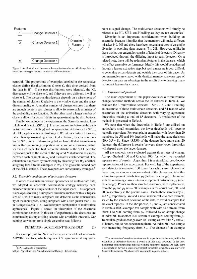
Over-sensitive(Always outputs

Change)

Over-conservative(Never outputs Change)

The ideal detector

Random detector

Figure 2: Scatterplot of the 88 detector methods in the space (ARL, TTD) for theAbrupt-change part of the experiment. The three individual detectors are highlighted.

MDR The percentage of runs for which the detector did not signalafter a true change.

Based on these characteristics, a good method should maximiseARL and NFA, and minimise TTD and MDR.

Figure 2 is the archetype of our result figures. It plots TTDversus ARL for the detection methods. The grey dots correspond toensemble methods, and the highlighted black dots correspond to theindividual detectors (Hotelling, KL, and SPLL). The ideal detectorwill have ARL=∞ (500 in our experiment, meaning that no falsedetection has been made before the true change happened), andTTD=0. This detector occupies the bottom right corner of the plot.

6

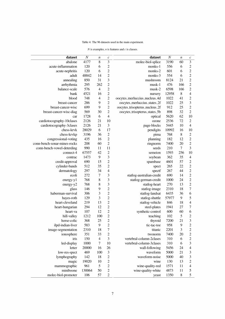
Table 4: The 96 datasets used in the main experiment.

N is examples, n is features and c is classes.

dataset N n cabalone 4177 8 3

acute-inflammation 120 6 2acute-nephritis 120 6 2

adult 48842 14 2annealing 850 31 3

arrhythmia 295 262 2balance-scale 576 4 2

bank 4521 16 2blood 748 4 2

breast-cancer 286 9 2breast-cancer-wisc 699 9 2

breast-cancer-wisc-diag 569 30 2car 1728 6 4

cardiotocography-10clases 2126 21 10cardiotocography-3clases 2126 21 3

chess-krvk 28029 6 17chess-krvkp 3196 36 2

congressional-voting 435 16 2conn-bench-sonar-mines-rocks 208 60 2

conn-bench-vowel-deterding 990 11 11connect-4 67557 42 2

contrac 1473 9 3credit-approval 690 15 2cylinder-bands 512 35 2

dermatology 297 34 4ecoli 272 7 3

energy-y1 768 8 3energy-y2 768 8 3

glass 146 9 2haberman-survival 306 3 2

hayes-roth 129 3 2heart-cleveland 219 13 2heart-hungarian 294 12 2

heart-va 107 12 2hill-valley 1212 100 2

horse-colic 368 25 2ilpd-indian-liver 583 9 2

image-segmentation 2310 18 7ionosphere 351 33 2

iris 150 4 3led-display 1000 7 10

letter 20000 16 26low-res-spect 469 100 3

lymphography 142 18 2magic 19020 10 2

mammographic 961 5 2miniboone 130064 50 2

molec-biol-promoter 106 57 2

dataset N n cmolec-biol-splice 3190 60 3

monks-1 556 6 2monks-2 601 6 2monks-3 554 6 2

mushroom 8124 21 2musk-1 476 166 2musk-2 6598 166 2nursery 12958 8 4

oocytes merluccius nucleus 4d 1022 41 2oocytes merluccius states 2f 1022 25 3

oocytes trisopterus nucleus 2f 912 25 2oocytes trisopterus states 5b 898 32 2

optical 5620 62 10ozone 2536 72 2

page-blocks 5445 10 4pendigits 10992 16 10

pima 768 8 2planning 182 12 2ringnorm 7400 20 2

seeds 210 7 3semeion 1593 256 10soybean 362 35 4

spambase 4601 57 2spect 265 22 2

spectf 267 44 2statlog-australian-credit 690 14 2

statlog-german-credit 1000 24 2statlog-heart 270 13 2

statlog-image 2310 18 7statlog-landsat 6435 36 6statlog-shuttle 57977 9 5statlog-vehicle 846 18 4

steel-plates 1941 27 7synthetic-control 600 60 6

teaching 102 5 2thyroid 7200 21 3

tic-tac-toe 958 9 2titanic 2201 3 2

twonorm 7400 20 2vertebral-column-2clases 310 6 2vertebral-column-3clases 310 6 3

wall-following 5456 24 4waveform 5000 21 3

waveform-noise 5000 40 3wine 130 13 2

wine-quality-red 1571 11 4wine-quality-white 4873 11 5

yeast 1350 8 5

7

Dots which are close to this corner are indicative of good detectors.The two trivial detectors lie at the two ends of the diagonal plotted

in the figure. A detector which always signals change has ARL=0and TTD=0, while detector which never signals change has ARL=

500 and TTD=500. A detector which signals change at randomwill have its corresponding point on the same diagonal. The exactposition on the diagonal will depend on the probability of signallinga change (unrelated to actual change). Denote this probability by p.Then ARL is the expectation of a random variable X with a geomet-ric distribution (X is the number of Bernoulli trials needed to get onesuccess, with probability of success p), that is ARL=

1−pp . The time

to detection, TTD, amounts to the same quantity because it is alsothe expected number of trials to the first success, with the same prob-ability of success p. Thus the diagonal ARL=TTD is a baseline forcomparing change detectors. A detector whose point lies above thediagonal is inadequate; it detects change when there is none, and failsto detect an existing change. We follow the same archetype for visu-alisation of the MDR/NFA space. We plot MDR against 1-NFA forthese figures in order to maintain the same visual orientation for per-formance. Therefore the ideal detector in this space is also at point(1,0), i.e., all changes were detected, and there were no false alarms.

3.4. A Case StudyIn addition to the main experiment, we conducted a practical

case study on a network intrusion detection dataset. We chosethe popular KDD Cup 1999 intrusion detection dataset, which isavailable from the UCI Machine Learning Repository [10]. Witha network intrusion dataset, the change context is more likely tobe longer-lived change from one concept to another, which could beeither abrupt or gradual. The dataset consists of 4,900,000 examplesand 42 features extracted from seven-weeks of TCP dump datafrom network traffic on a U.S. Air Force LAN. During the sevenweeks, the network was deliberately peppered with attacks whichfall into four main categories.

• Denial of Service (DOS): An attacker overwhelms computingresources in order to deny access to them.

• Remote to Login (R2L): Attempts at unauthorised access froma remote machine, such as guessing passwords.

• Unauthorized to Root (U2R): Unauthorised access to localsuperuser privileges, through a buffer overflow attack, forexample.

• Probing: Surveillance and investigation of weaknesses, suchas port scanning.

Of these categories, there are 24 specific attack concepts,or 24 classes. This dataset is most commonly interpreted as aclassification task. Viewed as such, it offers some interestingchallenges in its deficiencies. For example, there is 75% and 78%redundancy in duplicated records across the training and testingset respectively [52]. This can serve to bias learning algorithmstoward frequent records. It also has very imbalanced classes, withthe smurf and neptune DoS attacks constituting 71% of the datapoints; more than the ’normal’ class. We offer an interpretation ofthis data as a change detection task.

We evaluated the methods on the testing dataset. Since the datais sequential, we pass observations in order, one-by-one to each of

the detectors. The objective in our experiment was for the detectorsto identify the concept boundaries. When the concept changesfrom one class to another, we record whether this change pointwas detected. With this scheme, if we are experiencing a long-livedconcept such as a denial of service attack then after a sufficientnumber of examples of the same concept, we would expect thechange detection methods to also detect the changepoint back tothe normal class, or to another attack.

One challenge for the change detectors in this interpretation isthat some concepts may be very short-lived, that is, the change inthe distribution is a ‘blip’, involving only a few observations, afterwhich the distribution reverts back to the original one. Such blipsmay be too short to allow for detection by any method which isnot looking for isolated outliers.

4. Results and Discussion

Figure 3 visualises the ARL/TTD space for abrupt and gradualchange type by the categories in the taxonomy by Gama et al. [18].Each plot contains all 96 points (one for each data set) of the 88change detection methods. Empirically, there is a clear and visibledistinction between the methods in the Control Chart category,which performed, on average, worse than chance, and those in theother two categories. Table 5 confirms that Sequential Analysis andMonitoring distribution methods were much more likely to exhibit ahigh ARL. Furthermore, distribution monitoring methods exhibitedconsiderably lower TTD whilst being competitive on ARL withSequential Analysis methods. Observe the two distinct clusters inthe ARL/TTD space for this category (the triangle marker), andthe relative sparsity in-between. We suspect that this is the effectof gradual change on the TTD statistic. This is visible between thefigures, where we observe that, in the gradual change experiment,those methods with a high ARL and low TTD struggle to bettera TTD of 50, which is the halfway point of introducing the gradualchange. Those methods with an already low ARL do not movesignificantly in the TTD axis between experiments. We suspect thatthis is because a low ARL implies an over-eager detector, which inturn increases the probability that a valid detection is due to randomchance rather than a response to observation of the data.

The bottom two charts in Figure 3 visualise the NFA/MDR spacefor the aforementioned categories. Interestingly, we see a very sim-ilar effect for control chart methods. To understand why the perfor-mance of this category is so poor, we must consider the assumptionsof the detectors. This experiment presented the data points directlyto the change detection methods in the ensemble. Specifically, thiscategory contains EDDM, HDDMA and HDDMW , all of whichshare a common ancestor in DDM. Whilst the MOA interface forchange detectors accepts 64 bit floating point numbers, these meth-ods were not intended for continuous-valued data. As we mentionin subsection 3.1.2, DDM assumes the Binomial distribution. It alsoassumes that the monitored value (e.g., error rate of a classifier) willdecrease while the underlying distribution is stationary. The derivedmethods also share this assumption, which is fundamentally violatedby the nature of the data presented to them in this experiment.

The top 20 performers averaged over abrupt and gradual changeare summarised in the left half of Table 6. The performers were

8

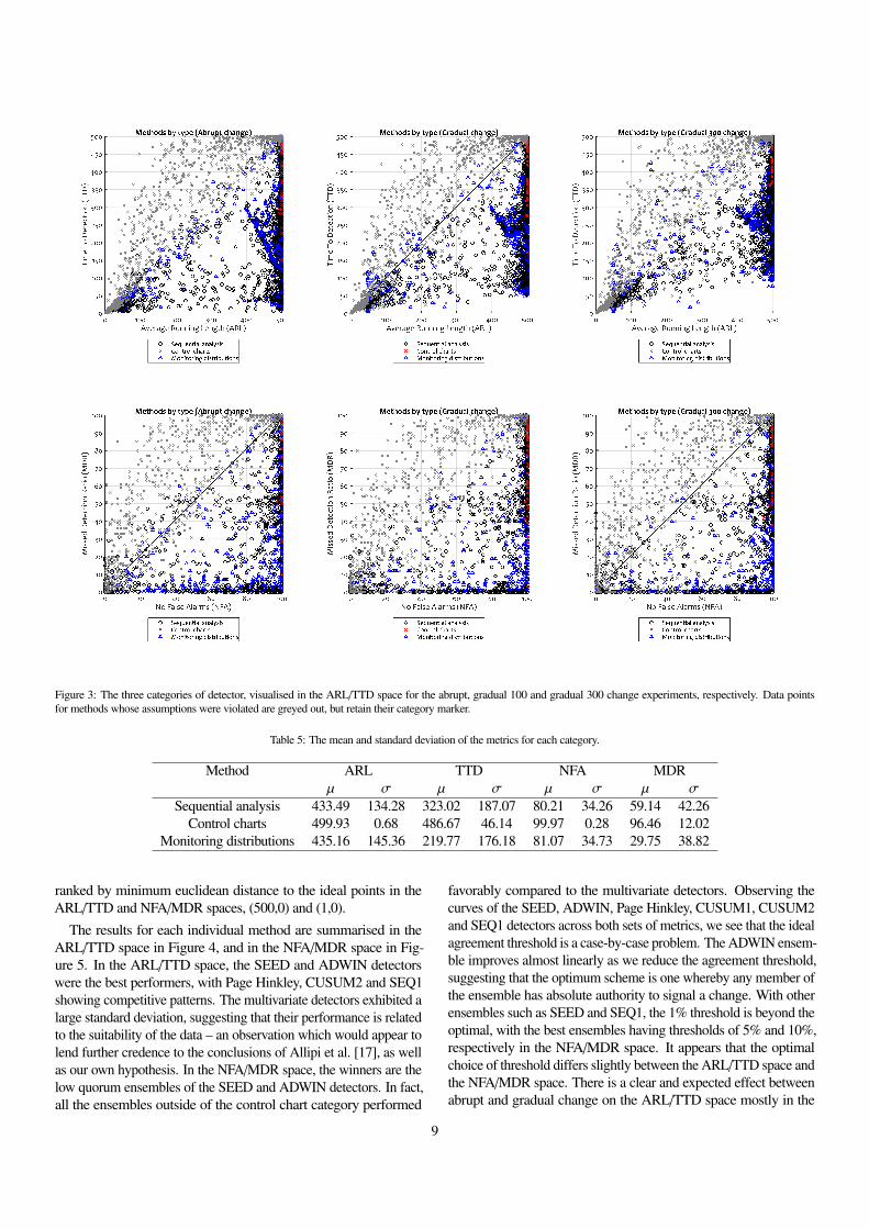
Figure 3: The three categories of detector, visualised in the ARL/TTD space for the abrupt, gradual 100 and gradual 300 change experiments, respectively. Data pointsfor methods whose assumptions were violated are greyed out, but retain their category marker.

Table 5: The mean and standard deviation of the metrics for each category.

Method ARL TTD NFA MDRµ σ µ σ µ σ µ σ

Sequential analysis 433.49 134.28 323.02 187.07 80.21 34.26 59.14 42.26Control charts 499.93 0.68 486.67 46.14 99.97 0.28 96.46 12.02

Monitoring distributions 435.16 145.36 219.77 176.18 81.07 34.73 29.75 38.82

ranked by minimum euclidean distance to the ideal points in theARL/TTD and NFA/MDR spaces, (500,0) and (1,0).

The results for each individual method are summarised in theARL/TTD space in Figure 4, and in the NFA/MDR space in Fig-ure 5. In the ARL/TTD space, the SEED and ADWIN detectorswere the best performers, with Page Hinkley, CUSUM2 and SEQ1showing competitive patterns. The multivariate detectors exhibited alarge standard deviation, suggesting that their performance is relatedto the suitability of the data – an observation which would appear tolend further credence to the conclusions of Allipi et al. [17], as wellas our own hypothesis. In the NFA/MDR space, the winners are thelow quorum ensembles of the SEED and ADWIN detectors. In fact,all the ensembles outside of the control chart category performed

favorably compared to the multivariate detectors. Observing thecurves of the SEED, ADWIN, Page Hinkley, CUSUM1, CUSUM2and SEQ1 detectors across both sets of metrics, we see that the idealagreement threshold is a case-by-case problem. The ADWIN ensem-ble improves almost linearly as we reduce the agreement threshold,suggesting that the optimum scheme is one whereby any member ofthe ensemble has absolute authority to signal a change. With otherensembles such as SEED and SEQ1, the 1% threshold is beyond theoptimal, with the best ensembles having thresholds of 5% and 10%,respectively in the NFA/MDR space. It appears that the optimalchoice of threshold differs slightly between the ARL/TTD space andthe NFA/MDR space. There is a clear and expected effect betweenabrupt and gradual change on the ARL/TTD space mostly in the

9

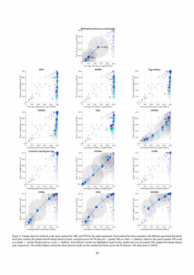
Figure 4: Change detection methods in the space spanned by ARL and TTD for the main experiment. Each method has been examined with different agreement thresholds.Each plot contains 88 gradual and 88 abrupt detector points, averaged across the 96 data sets – gradual 300 as a blue x (darkest), linked to the paired gradual 100 resultas a purple + and the abrupt result as a cyan * (lightest). Each detector’s points are highlighted, again in blue, purple and cyan for gradual 300, gradual and abrupt changetype, respectively. The shaded ellipses around the mean detector results are the standard deviations across the 96 datasets. The ideal point is (500,0).

10

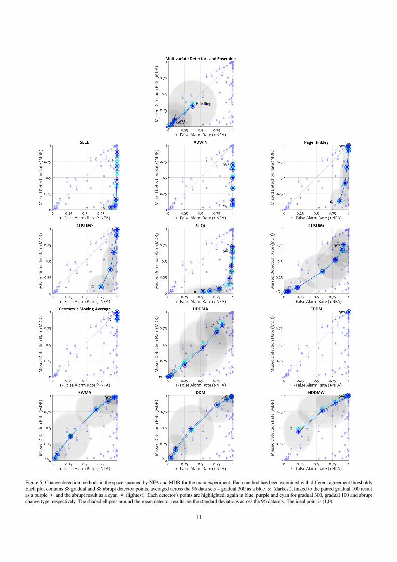
Figure 5: Change detection methods in the space spanned by NFA and MDR for the main experiment. Each method has been examined with different agreement thresholds.Each plot contains 88 gradual and 88 abrupt detector points, averaged across the 96 data sets – gradual 300 as a blue x (darkest), linked to the paired gradual 100 resultas a purple + and the abrupt result as a cyan * (lightest). Each detector’s points are highlighted, again in blue, purple and cyan for gradual 300, gradual 100 and abruptchange type, respectively. The shaded ellipses around the mean detector results are the standard deviations across the 96 datasets. The ideal point is (1,0).

11

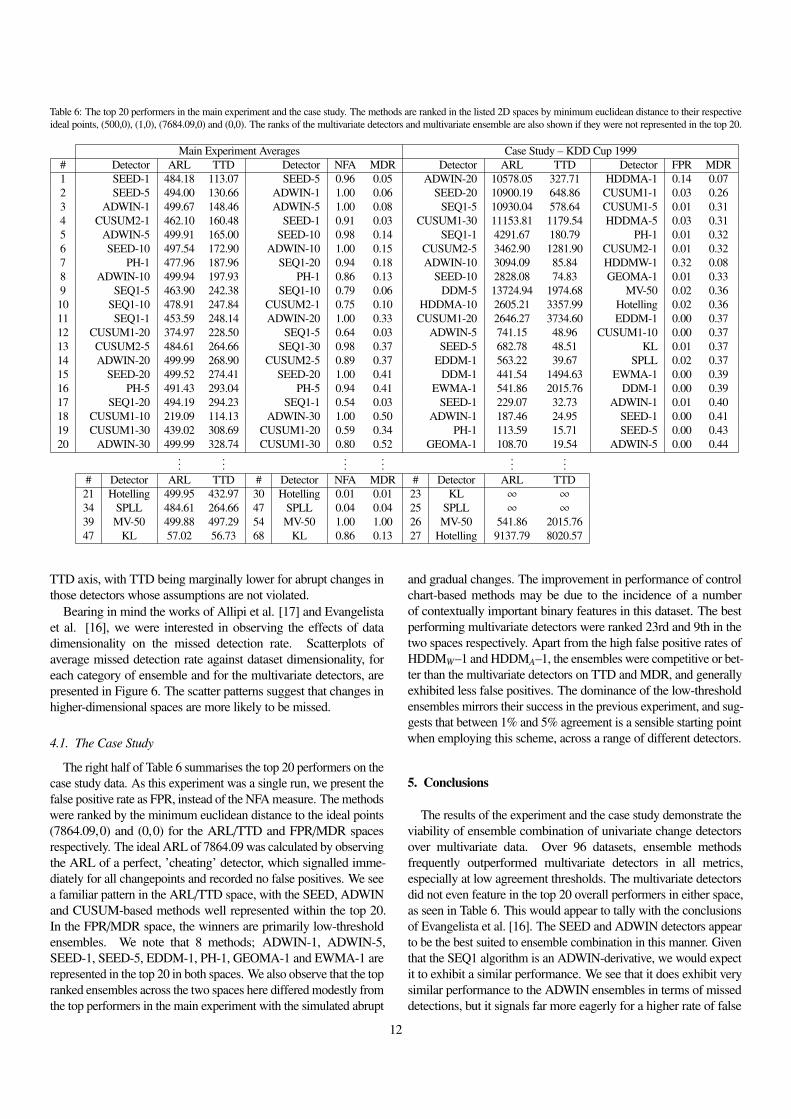
Table 6: The top 20 performers in the main experiment and the case study. The methods are ranked in the listed 2D spaces by minimum euclidean distance to their respectiveideal points, (500,0), (1,0), (7684.09,0) and (0,0). The ranks of the multivariate detectors and multivariate ensemble are also shown if they were not represented in the top 20.

Main Experiment Averages Case Study – KDD Cup 1999# Detector ARL TTD Detector NFA MDR Detector ARL TTD Detector FPR MDR1 SEED-1 484.18 113.07 SEED-5 0.96 0.05 ADWIN-20 10578.05 327.71 HDDMA-1 0.14 0.072 SEED-5 494.00 130.66 ADWIN-1 1.00 0.06 SEED-20 10900.19 648.86 CUSUM1-1 0.03 0.263 ADWIN-1 499.67 148.46 ADWIN-5 1.00 0.08 SEQ1-5 10930.04 578.64 CUSUM1-5 0.01 0.314 CUSUM2-1 462.10 160.48 SEED-1 0.91 0.03 CUSUM1-30 11153.81 1179.54 HDDMA-5 0.03 0.315 ADWIN-5 499.91 165.00 SEED-10 0.98 0.14 SEQ1-1 4291.67 180.79 PH-1 0.01 0.326 SEED-10 497.54 172.90 ADWIN-10 1.00 0.15 CUSUM2-5 3462.90 1281.90 CUSUM2-1 0.01 0.327 PH-1 477.96 187.96 SEQ1-20 0.94 0.18 ADWIN-10 3094.09 85.84 HDDMW-1 0.32 0.088 ADWIN-10 499.94 197.93 PH-1 0.86 0.13 SEED-10 2828.08 74.83 GEOMA-1 0.01 0.339 SEQ1-5 463.90 242.38 SEQ1-10 0.79 0.06 DDM-5 13724.94 1974.68 MV-50 0.02 0.3610 SEQ1-10 478.91 247.84 CUSUM2-1 0.75 0.10 HDDMA-10 2605.21 3357.99 Hotelling 0.02 0.3611 SEQ1-1 453.59 248.14 ADWIN-20 1.00 0.33 CUSUM1-20 2646.27 3734.60 EDDM-1 0.00 0.3712 CUSUM1-20 374.97 228.50 SEQ1-5 0.64 0.03 ADWIN-5 741.15 48.96 CUSUM1-10 0.00 0.3713 CUSUM2-5 484.61 264.66 SEQ1-30 0.98 0.37 SEED-5 682.78 48.51 KL 0.01 0.3714 ADWIN-20 499.99 268.90 CUSUM2-5 0.89 0.37 EDDM-1 563.22 39.67 SPLL 0.02 0.3715 SEED-20 499.52 274.41 SEED-20 1.00 0.41 DDM-1 441.54 1494.63 EWMA-1 0.00 0.3916 PH-5 491.43 293.04 PH-5 0.94 0.41 EWMA-1 541.86 2015.76 DDM-1 0.00 0.3917 SEQ1-20 494.19 294.23 SEQ1-1 0.54 0.03 SEED-1 229.07 32.73 ADWIN-1 0.01 0.4018 CUSUM1-10 219.09 114.13 ADWIN-30 1.00 0.50 ADWIN-1 187.46 24.95 SEED-1 0.00 0.4119 CUSUM1-30 439.02 308.69 CUSUM1-20 0.59 0.34 PH-1 113.59 15.71 SEED-5 0.00 0.4320 ADWIN-30 499.99 328.74 CUSUM1-30 0.80 0.52 GEOMA-1 108.70 19.54 ADWIN-5 0.00 0.44

......

......

......

# Detector ARL TTD # Detector NFA MDR # Detector ARL TTD21 Hotelling 499.95 432.97 30 Hotelling 0.01 0.01 23 KL ∞ ∞

34 SPLL 484.61 264.66 47 SPLL 0.04 0.04 25 SPLL ∞ ∞

39 MV-50 499.88 497.29 54 MV-50 1.00 1.00 26 MV-50 541.86 2015.7647 KL 57.02 56.73 68 KL 0.86 0.13 27 Hotelling 9137.79 8020.57

TTD axis, with TTD being marginally lower for abrupt changes inthose detectors whose assumptions are not violated.

Bearing in mind the works of Allipi et al. [17] and Evangelistaet al. [16], we were interested in observing the effects of datadimensionality on the missed detection rate. Scatterplots ofaverage missed detection rate against dataset dimensionality, foreach category of ensemble and for the multivariate detectors, arepresented in Figure 6. The scatter patterns suggest that changes inhigher-dimensional spaces are more likely to be missed.

4.1. The Case Study

The right half of Table 6 summarises the top 20 performers on thecase study data. As this experiment was a single run, we present thefalse positive rate as FPR, instead of the NFA measure. The methodswere ranked by the minimum euclidean distance to the ideal points(7864.09,0) and (0,0) for the ARL/TTD and FPR/MDR spacesrespectively. The ideal ARL of 7864.09 was calculated by observingthe ARL of a perfect, ’cheating’ detector, which signalled imme-diately for all changepoints and recorded no false positives. We seea familiar pattern in the ARL/TTD space, with the SEED, ADWINand CUSUM-based methods well represented within the top 20.In the FPR/MDR space, the winners are primarily low-thresholdensembles. We note that 8 methods; ADWIN-1, ADWIN-5,SEED-1, SEED-5, EDDM-1, PH-1, GEOMA-1 and EWMA-1 arerepresented in the top 20 in both spaces. We also observe that the topranked ensembles across the two spaces here differed modestly fromthe top performers in the main experiment with the simulated abrupt

and gradual changes. The improvement in performance of controlchart-based methods may be due to the incidence of a numberof contextually important binary features in this dataset. The bestperforming multivariate detectors were ranked 23rd and 9th in thetwo spaces respectively. Apart from the high false positive rates ofHDDMW–1 and HDDMA–1, the ensembles were competitive or bet-ter than the multivariate detectors on TTD and MDR, and generallyexhibited less false positives. The dominance of the low-thresholdensembles mirrors their success in the previous experiment, and sug-gests that between 1% and 5% agreement is a sensible starting pointwhen employing this scheme, across a range of different detectors.

5. Conclusions

The results of the experiment and the case study demonstrate theviability of ensemble combination of univariate change detectorsover multivariate data. Over 96 datasets, ensemble methodsfrequently outperformed multivariate detectors in all metrics,especially at low agreement thresholds. The multivariate detectorsdid not even feature in the top 20 overall performers in either space,as seen in Table 6. This would appear to tally with the conclusionsof Evangelista et al. [16]. The SEED and ADWIN detectors appearto be the best suited to ensemble combination in this manner. Giventhat the SEQ1 algorithm is an ADWIN-derivative, we would expectit to exhibit a similar performance. We see that it does exhibit verysimilar performance to the ADWIN ensembles in terms of misseddetections, but it signals far more eagerly for a higher rate of false

12

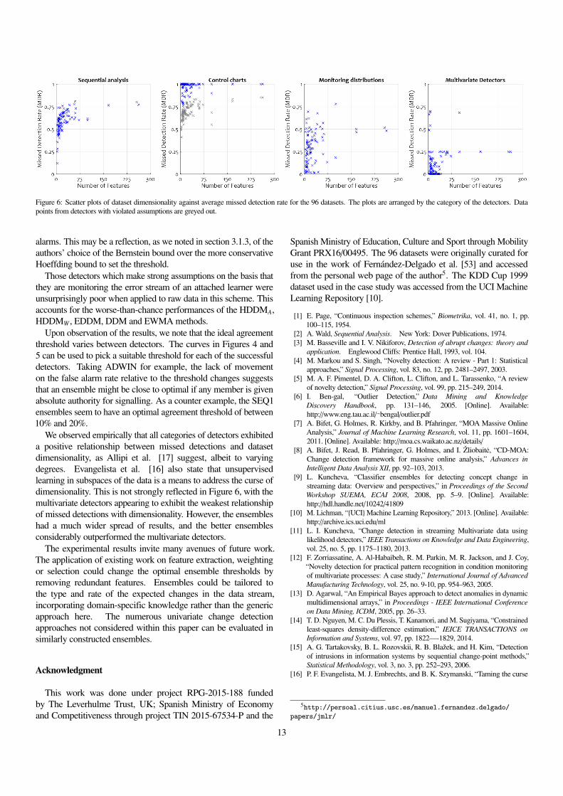
Figure 6: Scatter plots of dataset dimensionality against average missed detection rate for the 96 datasets. The plots are arranged by the category of the detectors. Datapoints from detectors with violated assumptions are greyed out.

alarms. This may be a reflection, as we noted in section 3.1.3, of theauthors’ choice of the Bernstein bound over the more conservativeHoeffding bound to set the threshold.

Those detectors which make strong assumptions on the basis thatthey are monitoring the error stream of an attached learner wereunsurprisingly poor when applied to raw data in this scheme. Thisaccounts for the worse-than-chance performances of the HDDMA,HDDMW , EDDM, DDM and EWMA methods.

Upon observation of the results, we note that the ideal agreementthreshold varies between detectors. The curves in Figures 4 and5 can be used to pick a suitable threshold for each of the successfuldetectors. Taking ADWIN for example, the lack of movementon the false alarm rate relative to the threshold changes suggeststhat an ensemble might be close to optimal if any member is givenabsolute authority for signalling. As a counter example, the SEQ1ensembles seem to have an optimal agreement threshold of between10% and 20%.

We observed empirically that all categories of detectors exhibiteda positive relationship between missed detections and datasetdimensionality, as Allipi et al. [17] suggest, albeit to varyingdegrees. Evangelista et al. [16] also state that unsupervisedlearning in subspaces of the data is a means to address the curse ofdimensionality. This is not strongly reflected in Figure 6, with themultivariate detectors appearing to exhibit the weakest relationshipof missed detections with dimensionality. However, the ensembleshad a much wider spread of results, and the better ensemblesconsiderably outperformed the multivariate detectors.

The experimental results invite many avenues of future work.The application of existing work on feature extraction, weightingor selection could change the optimal ensemble thresholds byremoving redundant features. Ensembles could be tailored tothe type and rate of the expected changes in the data stream,incorporating domain-specific knowledge rather than the genericapproach here. The numerous univariate change detectionapproaches not considered within this paper can be evaluated insimilarly constructed ensembles.

Acknowledgment

This work was done under project RPG-2015-188 fundedby The Leverhulme Trust, UK; Spanish Ministry of Economyand Competitiveness through project TIN 2015-67534-P and the

Spanish Ministry of Education, Culture and Sport through MobilityGrant PRX16/00495. The 96 datasets were originally curated foruse in the work of Fernandez-Delgado et al. [53] and accessedfrom the personal web page of the author5. The KDD Cup 1999dataset used in the case study was accessed from the UCI MachineLearning Repository [10].

[1] E. Page, “Continuous inspection schemes,” Biometrika, vol. 41, no. 1, pp.100–115, 1954.

[2] A. Wald, Sequential Analysis. New York: Dover Publications, 1974.[3] M. Basseville and I. V. Nikiforov, Detection of abrupt changes: theory and

application. Englewood Cliffs: Prentice Hall, 1993, vol. 104.[4] M. Markou and S. Singh, “Novelty detection: A review - Part 1: Statistical

approaches,” Signal Processing, vol. 83, no. 12, pp. 2481–2497, 2003.[5] M. A. F. Pimentel, D. A. Clifton, L. Clifton, and L. Tarassenko, “A review

of novelty detection,” Signal Processing, vol. 99, pp. 215–249, 2014.[6] I. Ben-gal, “Outlier Detection,” Data Mining and Knowledge

Discovery Handbook, pp. 131–146, 2005. [Online]. Available:http://www.eng.tau.ac.il/∼bengal/outlier.pdf

[7] A. Bifet, G. Holmes, R. Kirkby, and B. Pfahringer, “MOA Massive OnlineAnalysis,” Journal of Machine Learning Research, vol. 11, pp. 1601–1604,2011. [Online]. Available: http://moa.cs.waikato.ac.nz/details/

[8] A. Bifet, J. Read, B. Pfahringer, G. Holmes, and I. Zliobaite, “CD-MOA:Change detection framework for massive online analysis,” Advances inIntelligent Data Analysis XII, pp. 92–103, 2013.

[9] L. Kuncheva, “Classifier ensembles for detecting concept change instreaming data: Overview and perspectives,” in Proceedings of the SecondWorkshop SUEMA, ECAI 2008, 2008, pp. 5–9. [Online]. Available:http://hdl.handle.net/10242/41809

[10] M. Lichman, “{UCI}Machine Learning Repository,” 2013. [Online]. Available:http://archive.ics.uci.edu/ml

[11] L. I. Kuncheva, “Change detection in streaming Multivariate data usinglikelihood detectors,” IEEE Transactions on Knowledge and Data Engineering,vol. 25, no. 5, pp. 1175–1180, 2013.

[12] F. Zorriassatine, A. Al-Habaibeh, R. M. Parkin, M. R. Jackson, and J. Coy,“Novelty detection for practical pattern recognition in condition monitoringof multivariate processes: A case study,” International Journal of AdvancedManufacturing Technology, vol. 25, no. 9-10, pp. 954–963, 2005.

[13] D. Agarwal, “An Empirical Bayes approach to detect anomalies in dynamicmultidimensional arrays,” in Proceedings - IEEE International Conferenceon Data Mining, ICDM, 2005, pp. 26–33.

[14] T. D. Nguyen, M. C. Du Plessis, T. Kanamori, and M. Sugiyama, “Constrainedleast-squares density-difference estimation,” IEICE TRANSACTIONS onInformation and Systems, vol. 97, pp. 1822—-1829, 2014.

[15] A. G. Tartakovsky, B. L. Rozovskii, R. B. Blazek, and H. Kim, “Detectionof intrusions in information systems by sequential change-point methods,”Statistical Methodology, vol. 3, no. 3, pp. 252–293, 2006.

[16] P. F. Evangelista, M. J. Embrechts, and B. K. Szymanski, “Taming the curse

5http://persoal.citius.usc.es/manuel.fernandez.delgado/

papers/jmlr/

13

of dimensionality in kernels and novelty detection,” in Applied soft computingtechnologies: The challenge of complexity. Springer, 2006, pp. 425–438.

[17] C. Alippi, G. Boracchi, D. Carrera, and M. Roveri, “Change detection inmultivariate datastreams: likelihood and detectability loss,” in Proceedingsof the Twenty-Fifth International Joint Conference on Artificial Intelligence.AAAI Press, 2016, pp. 1368–1374.

[18] J. Gama, I. Zliobaite, A. Bifet, M. Pechenizkiy, and A. Bouchachia, “A surveyon concept drift adaptation,” ACM Computing Surveys, vol. 46, no. 4, pp. 1–37,2014.

[19] G. Ditzler, M. Roveri, C. Alippi, and R. Polikar, “Learning in nonstationaryenvironments: A survey,” IEEE Computational Intelligence Magazine, vol. 10,no. 4, pp. 12–25, 2015.

[20] L. Tarassenko, A. Hann, and D. Young, “Integrated monitoring and analysisfor early warning of patient deterioration.” British journal of anaesthesia,vol. 97, no. 1, pp. 64–8, jul 2006.

[21] X. Song, M. Wu, C. Jermaine, and S. Ranka, “Statistical changedetection for multi-dimensional data,” Proceedings of the 13th ACMSIGKDD international conference on Knowledge discovery and datamining - KDD ’07, vol. V, p. 667, 2007. [Online]. Available:http://portal.acm.org/citation.cfm?doid=1281192.1281264

[22] T. Dasu, S. Krishnan, S. Venkatasubramanian, and K. Yi, “An information-theoretic approach to detecting changes in multi-dimensional data streams,” inProc. Symp. on the Interface of Statistics, Computing Science, and Applications,2006.

[23] G. Krempl, Z. F. Siddiqui, and M. Spiliopoulou, “Online clustering ofhigh-dimensional trajectories under concept drift,” in Joint EuropeanConference on Machine Learning and Knowledge Discovery in Databases.Springer, 2011, pp. 261–276.

[24] M. M. Gaber and P. S. Yu, “Classification of changes in evolving data streamsusing online clustering result deviation,” in Proc. Of International Workshopon Knowledge Discovery in Data Streams, 2006.

[25] H. Hotelling, “The generalization of Student’s ratio,” in Breakthroughs inStatistics, 1992, pp. 54—-65.

[26] W. J. Faithfull and L. I. Kuncheva, “On optimum thresholding of multivariatechange detectors,” in Lecture Notes in Computer Science (including subseriesLecture Notes in Artificial Intelligence and Lecture Notes in Bioinformatics),vol. 8621 LNCS. Springer Verlag, 2014, pp. 364–373.

[27] B. Krawczyk, L. L. Minku, J. Gama, J. Stefanowski, and M. Wozniak,“Ensemble learning for data stream analysis: a survey,” Information Fusion,vol. 37, pp. 132–156, 2017.

[28] H. M. Gomes, J. P. Barddal, F. Enembreck, and A. Bifet, “A survey onensemble learning for data stream classification,” ACM Computing Surveys(CSUR), vol. 50, no. 2, p. 23, 2017.

[29] B. I. F. Maciel, S. G. T. C. Santos, and R. S. M. Barros, “ALightweight Concept Drift Detection Ensemble,” in 2015 IEEE27th International Conference on Tools with Artificial Intelligence(ICTAI). IEEE, nov 2015, pp. 1061–1068. [Online]. Available:http://ieeexplore.ieee.org/lpdocs/epic03/wrapper.htm?arnumber=7372248

[30] M. Wozniak, P. Ksieniewicz, B. Cyganek, and K. Walkowiak, “Ensemblesof heterogeneous concept drift detectors-experimental study,” in IFIPInternational Conference on Computer Information Systems and IndustrialManagement, ser. Lecture Notes in Computer Science, vol. 9842. Springer,2016, pp. 538–549.

[31] L. Du, Q. Song, L. Zhu, and X. Zhu, “A selective detector ensemble for conceptdrift detection,” The Computer Journal, vol. 58, no. 3, pp. 457–471, 2014.

[32] C. Alippi, G. Boracchi, and M. Roveri, “Hierarchical change-detection tests,”IEEE transactions on neural networks and learning systems, vol. 28, no. 2,pp. 246–258, 2017.

[33] A. Bifet, G. Holmes, B. Pfahringer, R. Kirkby, and R. Gavalda, “New ensemblemethods for evolving data streams,” in Proceedings of the 15th ACM SIGKDDInternational Conference on Knowledge Discovery and Data Mining. ACM,2009, pp. 139–148.

[34] A. Bifet, E. Frank, G. Holmes, and B. Pfahringer, “Accurate ensembles fordata streams: Combining restricted Hoeffding trees using stacking.” 2nd AsianConference on Machine Learning (ACML2010), pp. 1–16, 2010. [Online].Available: http://eprints.pascal-network.org/archive/00007198/

[35] ——, “Ensembles of restricted hoeffding trees,” Proceedings of the 14thInternational Conference on Artificial Intelligence and Statistics, vol. 15, no.212, pp. 434–442, 2012.

[36] I. Frias-Blanco, J. del Campo-Avila, G. Ramos-Jimenez, R. Morales-Bueno,A. Ortiz-Diaz, and Y. Caballero-Mota, “Online and non-parametric drift

detection methods based on Hoeffding’s bounds,” IEEE Transactions onKnowledge and Data Engineering, vol. 27, no. 3, pp. 810–823, 2015.

[37] J. Gama, P. Medas, G. Castillo, and P. Rodrigues, “Learning with driftdetection,” Advances in Artificial Intelligence – SBIA 2004, pp. 286–295, 2004.

[38] M. Baena-Garcıa, J. del Campo Avila, R. Fidalgo, A. Bifet, R. Gavalda, andR. Morales-Bueno, “Early Drift Detection Method,” Fourth internationalworkshop on knowledge discovery from data streams, vol. 6, pp. 77–86, 2006.

[39] W. N. Street and Y. Kim, “A streaming ensemble algorithm(SEA) for large-scale classification,” Proceedings of the seventh ACMSIGKDD international conference on Knowledge discovery and datamining - KDD ’01, vol. 4, pp. 377–382, 2001. [Online]. Available:http://portal.acm.org/citation.cfm?doid=502512.502568

[40] D. T. J. Huang, Y. S. Koh, G. Dobbie, and R. Pears, “Detecting volatilityshift in data streams,” in Data Mining (ICDM), 2014 IEEE InternationalConference on. IEEE, 2014, pp. 863–868.

[41] A. Bifet and R. Gavalda, “Learning from time-changing data with AdaptiveWindowing,” Proceedings of the 2007 SIAM International Conference on DataMining, pp. 443–448, 2007.

[42] S. Sakthithasan, R. Pears, and Y. S. Koh, “One pass concept change detectionfor data streams,” Advances in Knowledge Discovery and Data Mining, pp.461–472, 2013.

[43] G. J. Ross, N. M. Adams, D. K. Tasoulis, and D. J. Hand, “Exponentiallyweighted moving average charts for detecting concept drift,” PatternRecognition Letters, vol. 33, no. 2, pp. 191–198, 2012.

[44] S. W. Roberts, “Control chart tests based on geometric movingaverages,” Technometrics, vol. 3, pp. 239–250, 2012. [Online]. Available:http://dx.doi.org/10.2307/1271439

[45] H. Mouss, D. Mouss, N. Mouss, and L. Sefouhi, “Test of page-hinckley, anapproach for fault detection in an agro-alimentary production system,” inProceedings of the 5th Asian Control Conference, 2004, pp. 815–818.

[46] J. Gama, R. Sebastiao, and P. P. Rodrigues, “On evaluating stream learningalgorithms,” Machine learning, vol. 90, no. 3, pp. 317–346, 2013.

[47] R. Klinkenberg and T. Joachims, “Detecting concept drift with support vectormachines,” in Proceedings of ICML-00, 17th International Conference onMachine Learning, 2000, pp. 487–494.

[48] G. Widmer and M. Kubat, “Learning in the presence of concept drift andhidden contexts,” Machine Learning, vol. 23, no. 1, pp. 69–101, 1996.

[49] L. Kuncheva, “That elusive diversity in classifier ensembles,”in Iberian Conference on Pattern Recognition and Image, vol.2652. Springer, 2003, pp. 1126–1138. [Online]. Available:http://link.springer.com/chapter/10.1007/978-3-540-44871-6 130

[50] L. I. Kuncheva, Combining Pattern Classifiers: Methods and Algorithms:Second Edition. Wiley Blackwell, sep 2014.

[51] D. Brzezinski and J. Stefanowski, “Ensemble diversity in evolving datastreams,” in International Conference on Discovery Science, ser. Lecture Notesin Computer Science, vol. 9956. Springer, 2016, pp. 229–244.

[52] M. Tavallaee, E. Bagheri, W. Lu, and A. A. Ghorbani, “A detailed analysis ofthe kdd cup 99 data set,” in Computational Intelligence for Security and DefenseApplications, 2009. CISDA 2009. IEEE Symposium on. IEEE, 2009, pp. 1–6.

[53] M. Fernandez-Delgado, E. Cernadas, S. Barro, and D. Amorim, “Do we needhundreds of classifiers to solve real world classification problems,” Journalof Machine Learning Research, vol. 15, no. 1, pp. 3133–3181, 2014.

14