Computational Biology VI Jianfeng Feng Warwick University

Computational Biology VI

Jianfeng Feng

Warwick University

Our module

Preprocessing Data Analysis

Raw Data Acquisition

Slice-time Correction

Motion Correction, Co-registration & Normalization

Spatial Smoothing

Localizing Brain Activity

Applications:Clinical

Reconstruction

Data Processing Pipeline

Connectivity

Experimental Design

Linear Model

Grangercausality

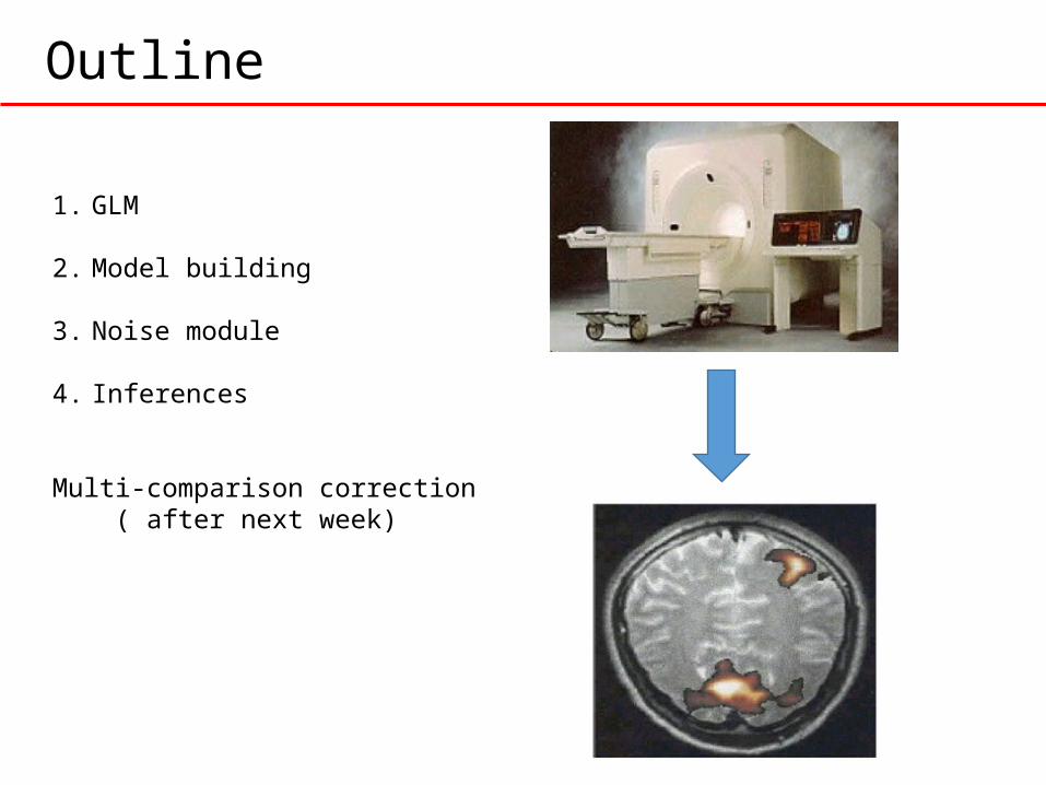
Outline

1. GLM

2. Model building

3. Noise module

4. Inferences

Multi-comparison correction ( after next week)

1: The General Linear Model

Statistical Analysis

• There are multiple goals in the statistical analysis or machine learning side of fMRI data.

• They include:

– localizing brain areas activated by the task;

– determining networks corresponding to brain function; and

– making predictions about psychological or disease states.

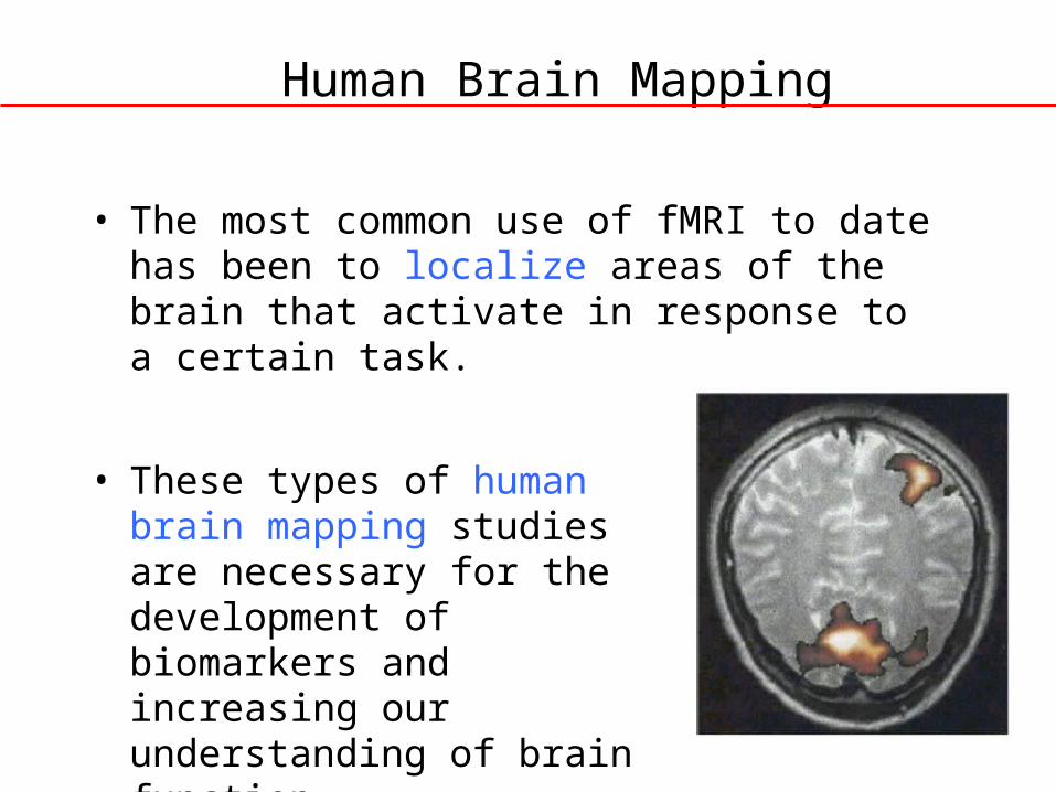
Human Brain Mapping

• The most common use of fMRI to date has been to localize areas of the brain that activate in response to a certain task.

• These types of human brain mapping studies are necessary for the development of biomarkers and increasing our understanding of brain function.

Massive Univariate Approach

• Typically analysis is performed by constructing a separate model at each voxel– The ‘massive univariate approach’.

– Assumes an improbable independence between voxel pairs......

• Typically dependencies between voxels are dealt with later using random field theory, which makes assumptions about the spatial dependencies between voxels.

General Linear Model

• The general linear model (GLM) approach treats the data as a linear combination of model functions (predictors) plus noise (error).

• The model functions are assumed to have known shapes, but their amplitudes are unknown and need to be estimated.

• The GLM framework encompasses many of the commonly used techniques in fMRI data analysis (and big data analysis more generally).

y(t) = b0 + b1 f1(t) +… + + bp fp(t) + e(t)

• Consider an experiment of alternating blocks of finger-tapping and rest.

• Construct a model to study data from a single voxel for a single subject.

• We seek to determine whether activation is higher during finger-tapping compared with rest.

Illustration

fMRI Data Design matrix Model parameters

Residuals

BOLD signal Intercept Predicted task response

= X +[𝛽0

𝛽1]

10

301

300

2

1

01

01

11

11

11

01

01

01

x

y

y

y

y

y

N


Residuals

= X +[𝛽0

𝛽1]

In simple formula: y(t) = b0 + b1 f1(t) + e1(t)


Residuals


= X +

H0 : 1 0

Null hypothesis

[𝛽0

𝛽1]

where

fMRI Data Design matrix

Regression coefficients

GLM

A standard GLM can be written:

y(t) = b0 + b1 f1(t) +… + + bp fp(t) + e(t) or

Y Xβ ε

Noise

ε ~ N (0, V)

V is the covariance matrix whose format depends on the noise model.

The quality of the model depends on our choice of X and V.

In matrix format (lecture 4, time series)

For k dimensional case

where the recorded data (Y(1), Y(2), Y(3), …, Y(T)), denoting

Problem Formulation

• Assume the model:

• The matrices X and Y are assumed to be known, and the noise is considered to be uncorrelated.

• Our goal is to find the value of that minimizes:

y XβT y Xβ

Y Xβ ε ε ~ N(0, I 2 )

OLS Solution

Ordinary least squares solution

βˆ (XT X)1 XT y

Properties:

Maximum likelihood estimate

E ˆ

Var(ˆ) 2 XT X

1

Can we do better?

Gauss Markov Theorem

• The Gauss-Markov Theorem states that any other unbiased estimator of will have a larger variance than the OLS solution.

• Assume is an unbiased estimator of .

• Then according to G-M Theorem,

Var() Var()

• ˆ is the best linear unbiased estimator (BLUE) of .

Estimation

• If is i.i.d., then Ordinary Least Square (OLS) estimate is optimal

• If Var() =V2 I2, then Generalized Least Squares (GLS) estimate is optimal

Y Xβ εestimate

βˆ (X' X)1 X' Y

estimate

βˆ (X' V 1X)1 X' V 1Y

Y Xβ ε

model

model

Summary

estimate

βˆ (X' V 1X)1 X' V 1Y

model

Y Xβ ε

fitted values

Yˆ

Xˆ

r Y

Yˆ

(I (X ' V1X)1

X ' V1 )Y

RY

residuals

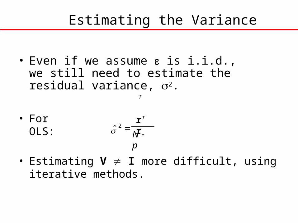
Estimating the Variance

• Even if we assume is i.i.d., we still need to estimate the residual variance, 2.

• For OLS:

• Estimating V I more difficult, using iterative methods.

T

N p

rT r̂

2

Estimation

• If is i.i.d., then Ordinary Least Square (OLS) estimate is optimal

• If Var() =V2 I2, then Generalized Least Squares (GLS) estimate is optimal

Y Xβ εestimate

βˆ (X' X)1 X' Y

estimate

βˆ (X' V 1X)1 X' V 1Y

Y Xβ ε

model

model

Model Refinement

• This model has a number of shortcomings.

• We want to use our understanding of the signal and noise properties of BOLD fMRI to aid us in constructing appropriate models.

• This includes deciding on an appropriate design matrix, as well as an appropriate noise model.

Issues

1. BOLD responses have a

delayed and dispersed form.

2. The fMRI signal includes substantial amounts of low- frequency noise.

3. The data are serially correlated which needs to be considered in the model.

clear allclose allfor i=1:400 h=0.1; x(i)=i*h; y(i)=x(i)*x(i)*x(i)*x(i)*exp(-x(i));endfor i=41:350 m(i)=y(i-40); y(i)=y(i)-m(i)*0.2;end plot(x([1:300]),y([1:300])/max(y))

2: Model Building


Y Xβ εwhere


Model parameters

Noise

General Linear Model



ε ~ N (0, V)

Model Building

• Proper construction of the design matrix is critical for effective use of the GLM.

• This process can be complicated by the following properties of the BOLD response:– It includes low-frequency noise and artifacts related to

head movement and cardiopulmonary-induced brain movement.

– The neural response shape may not be known.

– The hemodynamic response varies in shape across the brain.

BOLD Response

• Predict the shape of the BOLD response to a given stimulus pattern. Assume the shape is known and the amplitude is unknown.

• The relationship between stimuli and the BOLD response is typically modeled using a linear time invariant (LTI) system.

• In an LTI system an impulse (i.e., neuronal activity) is convolved with an impulse response function (i.e., HRF).

Convolution Examples

Hemodynamic Response Function

Predicted Response

Block Design

Experimental Stimulus Function

HRF Models

• Often a fixed canonical HRF is used to model the response to neuronal activity

- Linear combination of 2 gamma functions.

- Optimal if correct.

- If wrong, leads to bias

and power loss. Unlikely that the same HRF

is valid for all voxels.

True response may be faster/slower

True response may have smaller/bigger undershoot


Residuals


= X +

H : 001

[𝛽0

𝛽1]

Example

ModelImage of

predictors Data & Fitted

Single HRF


Residuals


= X +

H : 001

[𝛽0

𝛽1]

Example

In mathematical term, we have

y(t) = b0 + b1 f1(t) + e(t) or

Y Xβ ε

Checkerboard Thermal pain

Aversive picture, Aversive anticipation

Stimulus On

The HRF shape depends both on the vasculature and the time course of neural activity.

Problems

Assuming a fixed HRF is usually not appropriate.

Temporal Basis Functions

• To allow for different types of HRFs in different brain regions, it is typically better to use temporal basis functions.

• A linear combination of functions can be used to account for delays and dispersions in the HRF.– The stimulus function is convolved with each of the

basis functions to give a set of regressors.

– The parameter estimates give the coefficients that determine the combination of basis functions that best models the HRF for the trial type and voxel in question.

• In an LTI system the BOLD response is modeled

x(t) (s h)(t)

where s(t) is a stimulus function and h(t) the HRF and * is the convolution.

• Model the HRF as a linear combination of temporal basis functions, fi(t), such that

h(t) i fi (t)


h(t) i fi (t)


1

2

3

h(t)

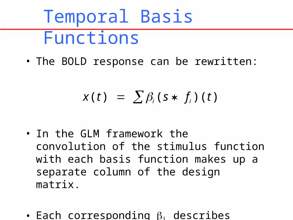
• The BOLD response can be rewritten:

x(t) i (s fi )(t)

• In the GLM framework the convolution of the stimulus function with each basis function makes up a separate column of the design matrix.

• Each corresponding i describes the weight of that component.



• Typically-used models vary in the degree they make a priori assumptions about the shape of the response.

• In the most extreme case, the shape of the HRF is fixed and only the amplitude is allowed to vary.

• By contrast, a finite impulse response (FIR) basis set, contains one free parameter for every time- point following stimulation for every cognitive event type.

The model estimates an HRF of arbitrary shape for each event type in each voxel of the brain

Finite Impulse Response

Basis sets

Time (s)

ModelImage ofpredictors Data & Fitted

Single HRF

HRF +derivatives

Finite Impulse Response (FIR)

Basis sets

Time (s)

ModelImage ofpredictors Data & Fitted

Single HRF

HRF +derivatives

Finite Impulse Response (FIR)

Overfitting ?????

Nuisance Covariates

• Often model factors associated with known sources of variability, but that are not related to the experimental hypothesis, need to be included in the GLM.

• Examples of possible ‘nuisance regressors’:– Signal drift

– Physiological (e.g., respiration) artifacts

– Head motion, e.g. six regressors comprising of three translations and three rotations.

Sometimes transformations of the six regressors also included.

• Slow changes in voxel intensity over time (low- frequency noise) is present in the fMRI signal.

• Scanner instabilities and not motion or physiological noise may be the main cause of the drift, as drift has been seen in cadavers.

• Need to include drift parameters in our models.- Use splines, polynomial basis or discrete cosine basis

Drift

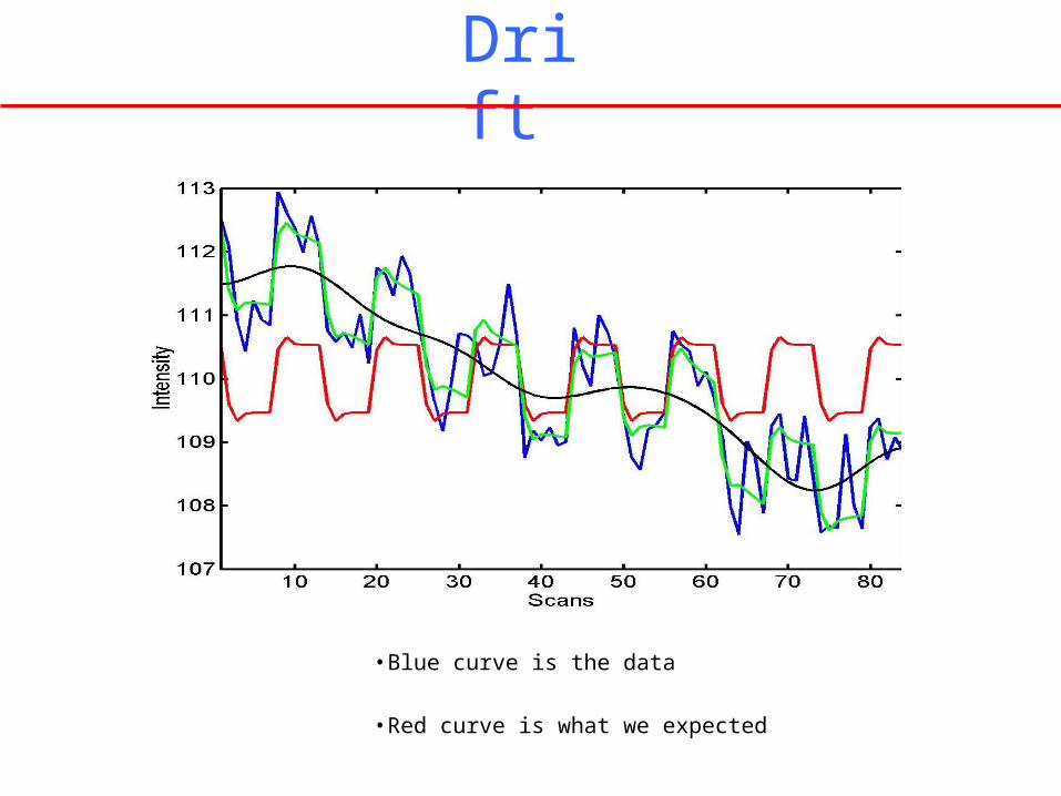
• Blue curve is the data

• Red curve is what we expected

Drift

=

+

= +Y X

Model with Drift

• Selecting fi as cos(i w t) and sin(i w t) for example (as in MP3, only cos is used)

blue =

black =

green =

data

mean + low-frequency drift predicted response, taking into account low-frequency drift

predicted response (with low- frequency drift explained away)

red =

High Pass Filtering

• Respiration and heart beat give rise to high- frequency noise.

• This type of noise is difficult to remove and is often left in the data giving rise to temporal autocorrelations.

Physiological Noise

3: Noise Models

where


Regression coefficients

GLM


Y Xβ ε

Noise

ε ~ N (0, V)



Design Matrix

• We has previously discussed various signal and nuisance components that can be included in the design matrix to improve the model.– Temporal Basis functions

Allows for flexible HRF

– Motion parameters Corrects for ‘spin history’ artifacts

fMRI Noise

• Functional MRI data typically exhibit significant autocorrelation.

– Caused by physiological noise and low frequency drift, that has not been appropriately modeled.

– Typically modeled using either an AR(p) process.

– Single subject statistics are not valid without an accurate model of the noise.

AR(1) model

• Serial correlation can be modeled using a first-order autoregressive model, i.e.

• The error term t depends on the previous error term t-1 and a new disturbance term ut.

t t1 ut ut ~ N (0, )2

AR(1) model

• The autocorrelation function (ACF) for an AR(1) process:

5 1 0 1 5

- 1. 0

- 0. 5

0. 00. 5

1. 0

1 :1 6

=0.7

𝜌 (h )={1 , i f h 0 , | h | i f h 0

IID Case AR(1) Case

Error Term

• The format of V will depend on what noise model is used.

GLM Summary

estimate

βˆ (X' V 1X)1 X' V 1Y

model

Y Xβ ε

fitted values

Yˆ

Xˆ

r Y

Yˆ

(I (X ' V1X)1

X ' V1 )Y

RY

residuals

Estimating V

• In general the form of the covariance matrix is unknown, which means it has to be estimated.

• Estimating V depends on ’s, and estimating’s depends on V. Need iterative procedure.

estimated covariance matrix from step 2.

Iterative Procedure

1. Assume that V=I and calculate the OLS solution.

2. Estimate the parameters of V using the residuals.

3. Re-estimate the values using the

4. Iterate until convergence.

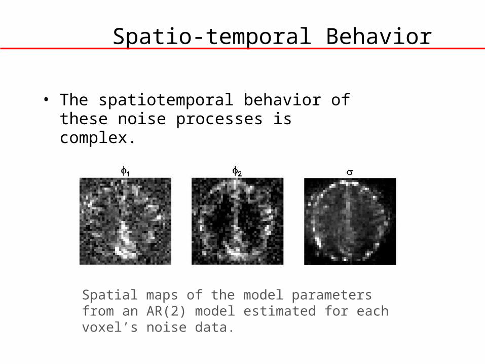
Spatio-temporal Behavior

• The spatiotemporal behavior of these noise processes is complex.

Spatial maps of the model parameters from an AR(2) model estimated for each voxel’s noise data.

4: Inference

GLM Summary

estimate

βˆ (X' V 1X)1 X' V 1Y

model

Y Xβ ε

fitted values

Yˆ

Xˆ

r Y

Yˆ

(I (X ' V1X)1

X ' V1 )Y

RY

residuals

• After fitting the GLM use the estimated parameters to determine whether there is significant activation present in the voxel.

• Inference is based on the fact that:

ˆ ~ N (, (XT V1X)1 )

• Use t or F test to perform tests on effects of interest.

Inference

Contrasts

• It is often of interest to see whether a linear combination of the parameters are significant.

• The term cT specifies a linear combination of the estimated parameters, i.e.

• Here c is called a contrast vector.

1 1 2 2 n nT

c β c c … c

• Experiment with two types of stimuli.

=

+ Noise

1

2

3

Example

H0 : 2 3

H0 : c β 0T

0, 1, 1

cT

H0 : cβ 0

use the t-statistic:

T Ha : c β 0T

Var cT βˆ

cT

βˆT

T-test

• To test

• Under H0, T is approximately t() with tr((RV))

(tr(RV))2 2

Multiple Contrasts

• We often want to make simultaneous tests of several contrasts at once.

• c is now a contrast matrix.

• Suppose

then

𝑪=(1 0 0 0 00 1 0 0 0)

=

+

= +Y X

Consider a model with box-car shaped activation and drift modeled using the discrete cosine basis.

Example

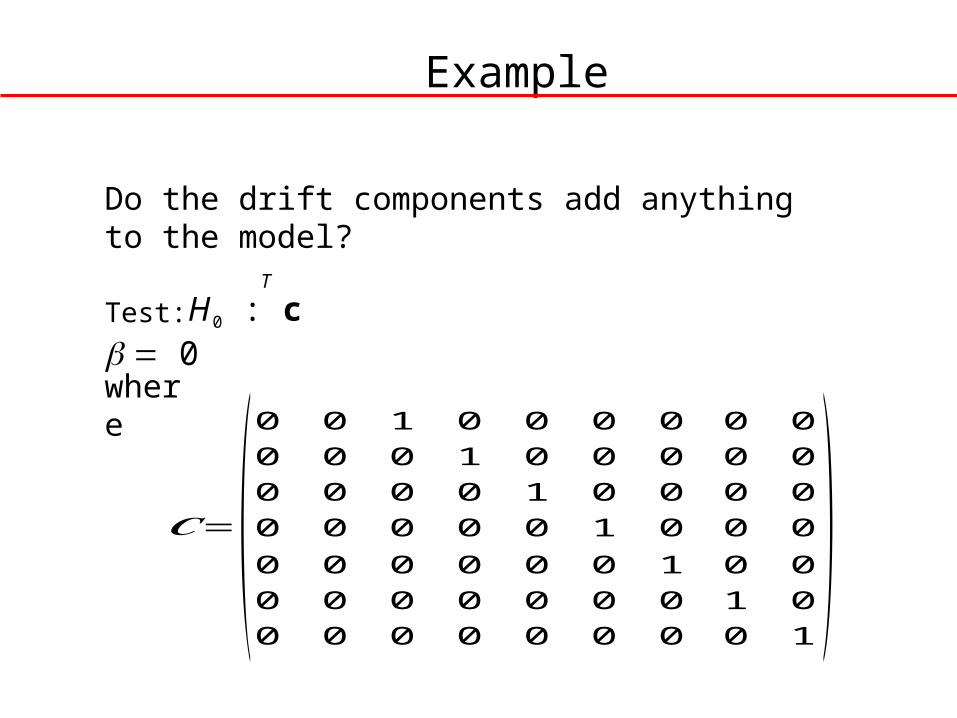
Do the drift components add anything to the model?

Test: H0 : c 0T

where

Example

𝑪=(0 0 1 0 0 0 0 0 00 0 0 1 0 0 0 0 00 0 0 0 1 0 0 0 00 0 0 0 0 1 0 0 00 0 0 0 0 0 1 0 00 0 0 0 0 0 0 1 00 0 0 0 0 0 0 0 1

)

This is equivalent to testing:

H : 0T

89

7650 34

To understand what this implies, we split the design matrix into two parts:

X 0X 1

Example

[1 𝑋 11 𝑋 12 ⋯ 𝑋19

1 𝑋 21 𝑋 22 ⋯ 𝑋 29

⋮ ⋮ ⋮ ¿ ¿𝑋𝑛1¿𝑋𝑛2¿⋯¿𝑋𝑛9¿ ]

Example

• Do the drift components add anything to the model?

• The X1 matrix explains the drift. Does it contribute in a significant way to the model?

• Compare the results using the full model, with design matrix X, with those obtained using a reduced model, with design matrix X0.

r r r

r tr((R

R)Vˆ 0

2

00F TT

tr(R R

)Vtr(R R

)V 2

0

20

0 tr(RV)2

tr((RV)2 )

and

F-test

• Test the hypothesis using the F-statistic:

• Assuming the errors are normally distributed, F has an approximate F-distribution with (0,) degrees of freedom, where

Statistical Images

• For each voxel a hypothesis test is performed. The statistic corresponding to that test is used to create a statistical image over all voxels.

T-value

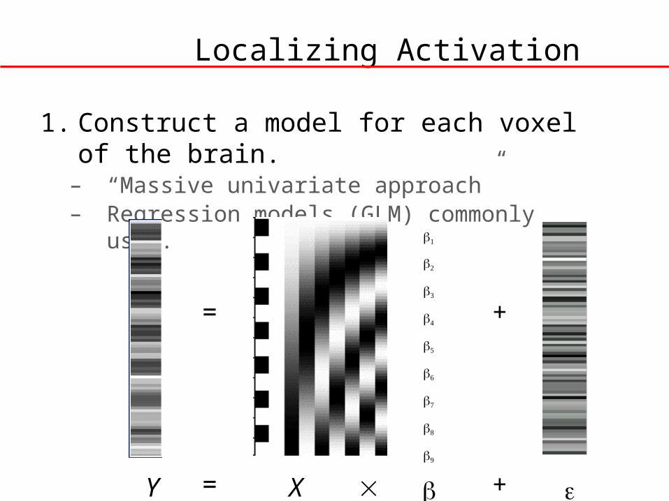
Localizing Activation

1. Construct a model for each voxel of the brain.– “Massive univariate approach”– Regression models (GLM) commonly used.

=

+

= +Y X


2. Perform a statistical test to determine whether task related activation is present in the voxel.

TH : c β 00

Statistical image: Map of t-tests across all voxels (a.k.a t-map).


3. Choose an appropriate threshold for determining statistical significance.

Statistical parametric map: (SPM) Each significant voxel is color-coded according to the size of its p-value.

How do we determine which voxels are actually active?

Problems:

• The statistics are obtained by performing a large number of hypothesis tests.

• Many of the test statistics will be artificially inflated due to the noise.

• This leads to many false positives.

Statistical Images

Multiple Comparisons

• Which of 100,000 voxels are significant?

– =0.05 5,000 false positive voxels

• Choosing a threshold is a balance

between sensitivity (true positive rate)

and specificity (true negative rate).

t > 1 t > 2 t > 3 t > 4 t > 5

Documents

Computational Biology VI Jianfeng Feng Warwick University