Embed Size (px)
Citation preview

Conformal Loop Ensembles andthe Gaussian Free Field
Sam WatsonPuMaGraSS
14 October, 2011

SLE
Introduction
What is the Schramm-Loewner evolution?
SLE(κ) is a non-self-crossing random fractal curve in a planardomain, from one boundary point to another (chordal) orfrom a boundary point to an interior point (radial)
Sample SLE traces from 0 to ∞ in the upper half-plane:
0∑= 8/3
0∑= 4
0∑= 6

SLE
Introduction
What is the Schramm-Loewner evolution?
SLE(κ) is a non-self-crossing random fractal curve in a planardomain, from one boundary point to another (chordal) orfrom a boundary point to an interior point (radial)
Sample SLE traces from 0 to ∞ in the upper half-plane:
0∑= 8/3
0∑= 4
0∑= 6

SLE
Introduction
A scaling limit of discrete paths
Brownian motion arises as a natural limit of random walks
Simple Random Walk Brownian Motion
Analogously, SLE arises as a natural limit for a variety ofdiscrete non-self-intersecting paths
Self-avoiding Walk SLE

SLE
Introduction
A scaling limit of discrete paths
Brownian motion arises as a natural limit of random walks
Simple Random Walk Brownian Motion
Analogously, SLE arises as a natural limit for a variety ofdiscrete non-self-intersecting paths
Self-avoiding Walk SLE

SLE
Introduction
A scaling limit of discrete paths
SLE arises in many two-dimensional probabilistic models
Loop-erased random walk, κ = 2 [Lawler, Schramm, Werner]Boundary of Brownian motion, κ = 8/3 [Lawler, Schramm,Werner]Ising model interface , κ = 3 [Smirnov, Chelkak and Hongler,Kytola]Level lines of DGFF, κ = 4, [Schramm and Sheffield]Percolation interface, κ = 6, [Smirnov and Camia, Newman]Uniform spanning tree, κ = 8, [Lawler, Schramm, Werner]
We will discuss percolation and the DGFF

SLE
Introduction
A scaling limit of discrete paths
SLE arises in many two-dimensional probabilistic models
Loop-erased random walk, κ = 2 [Lawler, Schramm, Werner]
Boundary of Brownian motion, κ = 8/3 [Lawler, Schramm,Werner]Ising model interface , κ = 3 [Smirnov, Chelkak and Hongler,Kytola]Level lines of DGFF, κ = 4, [Schramm and Sheffield]Percolation interface, κ = 6, [Smirnov and Camia, Newman]Uniform spanning tree, κ = 8, [Lawler, Schramm, Werner]
We will discuss percolation and the DGFF

SLE
Introduction
A scaling limit of discrete paths
SLE arises in many two-dimensional probabilistic models
Loop-erased random walk, κ = 2 [Lawler, Schramm, Werner]Boundary of Brownian motion, κ = 8/3 [Lawler, Schramm,Werner]
Ising model interface , κ = 3 [Smirnov, Chelkak and Hongler,Kytola]Level lines of DGFF, κ = 4, [Schramm and Sheffield]Percolation interface, κ = 6, [Smirnov and Camia, Newman]Uniform spanning tree, κ = 8, [Lawler, Schramm, Werner]
We will discuss percolation and the DGFF

SLE
Introduction
A scaling limit of discrete paths
SLE arises in many two-dimensional probabilistic models
Loop-erased random walk, κ = 2 [Lawler, Schramm, Werner]Boundary of Brownian motion, κ = 8/3 [Lawler, Schramm,Werner]Ising model interface , κ = 3 [Smirnov, Chelkak and Hongler,Kytola]
Level lines of DGFF, κ = 4, [Schramm and Sheffield]Percolation interface, κ = 6, [Smirnov and Camia, Newman]Uniform spanning tree, κ = 8, [Lawler, Schramm, Werner]
We will discuss percolation and the DGFF

SLE
Introduction
A scaling limit of discrete paths
SLE arises in many two-dimensional probabilistic models
Loop-erased random walk, κ = 2 [Lawler, Schramm, Werner]Boundary of Brownian motion, κ = 8/3 [Lawler, Schramm,Werner]Ising model interface , κ = 3 [Smirnov, Chelkak and Hongler,Kytola]Level lines of DGFF, κ = 4, [Schramm and Sheffield]
Percolation interface, κ = 6, [Smirnov and Camia, Newman]Uniform spanning tree, κ = 8, [Lawler, Schramm, Werner]
We will discuss percolation and the DGFF

SLE
Introduction
A scaling limit of discrete paths
SLE arises in many two-dimensional probabilistic models
Loop-erased random walk, κ = 2 [Lawler, Schramm, Werner]Boundary of Brownian motion, κ = 8/3 [Lawler, Schramm,Werner]Ising model interface , κ = 3 [Smirnov, Chelkak and Hongler,Kytola]Level lines of DGFF, κ = 4, [Schramm and Sheffield]Percolation interface, κ = 6, [Smirnov and Camia, Newman]
Uniform spanning tree, κ = 8, [Lawler, Schramm, Werner]
We will discuss percolation and the DGFF

SLE
Introduction
A scaling limit of discrete paths
SLE arises in many two-dimensional probabilistic models
Loop-erased random walk, κ = 2 [Lawler, Schramm, Werner]Boundary of Brownian motion, κ = 8/3 [Lawler, Schramm,Werner]Ising model interface , κ = 3 [Smirnov, Chelkak and Hongler,Kytola]Level lines of DGFF, κ = 4, [Schramm and Sheffield]Percolation interface, κ = 6, [Smirnov and Camia, Newman]Uniform spanning tree, κ = 8, [Lawler, Schramm, Werner]
We will discuss percolation and the DGFF

SLE
Introduction
A scaling limit of discrete paths
SLE arises in many two-dimensional probabilistic models
Loop-erased random walk, κ = 2 [Lawler, Schramm, Werner]Boundary of Brownian motion, κ = 8/3 [Lawler, Schramm,Werner]Ising model interface , κ = 3 [Smirnov, Chelkak and Hongler,Kytola]Level lines of DGFF, κ = 4, [Schramm and Sheffield]Percolation interface, κ = 6, [Smirnov and Camia, Newman]Uniform spanning tree, κ = 8, [Lawler, Schramm, Werner]
We will discuss percolation and the DGFF

SLE
Discrete models
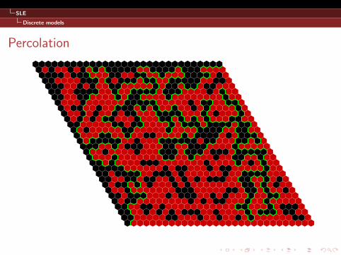
Percolation

SLE
Discrete models
Percolation
SLE
Discrete models
Percolation

SLE
Discrete models
Percolation

SLE
Discrete models
Percolation

SLE
Discrete models
Percolation
Theorem (Smirnov, 2001)
As the mesh size goes to 0, the law of the percolation interfacepath converges to SLE(6)
We’re thinking of the sample paths of the interfaces andSLE(6) as elements of the metric space of equivalence classesof curves from a to b modulo reparametrization, with metric
d([γ], [γ ′]) = infϕ
supu∈[0,1]
∣∣γ(u)− γ′(ϕ(u))
∣∣
Hence the laws of the interfaces and SLE(6) are measures onthis metric space with its Borel σ -algebra

SLE
Discrete models
Percolation
Theorem (Smirnov, 2001)
As the mesh size goes to 0, the law of the percolation interfacepath converges to SLE(6)
We’re thinking of the sample paths of the interfaces andSLE(6) as elements of the metric space of equivalence classesof curves from a to b modulo reparametrization, with metric
d([γ], [γ ′]) = infϕ
supu∈[0,1]
∣∣γ(u)− γ′(ϕ(u))
∣∣Hence the laws of the interfaces and SLE(6) are measures onthis metric space with its Borel σ -algebra

SLE
Discrete models
The Discrete Gaussian Free Field
The discrete Gaussian free field h is a random real-valuedfunction on a finite vertex set D⊂ Z2.
h is required to agree with some specified functionψ : ∂D→ R, and its density is given by
Z−1 exp
(−1
2 ∑x∼y
(h(x)−h(y))2
),
where the sum is over all pairs of neighbors in D.So the DGFF is a multivariate Gaussian in R|D|−|∂D|.

SLE
Discrete models
The Discrete Gaussian Free Field
The discrete Gaussian free field h is a random real-valuedfunction on a finite vertex set D⊂ Z2.h is required to agree with some specified functionψ : ∂D→ R, and its density is given by
Z−1 exp
(−1
2 ∑x∼y
(h(x)−h(y))2
),
where the sum is over all pairs of neighbors in D.
So the DGFF is a multivariate Gaussian in R|D|−|∂D|.

SLE
Discrete models
The Discrete Gaussian Free Field
The discrete Gaussian free field h is a random real-valuedfunction on a finite vertex set D⊂ Z2.h is required to agree with some specified functionψ : ∂D→ R, and its density is given by
Z−1 exp
(−1
2 ∑x∼y
(h(x)−h(y))2
),
where the sum is over all pairs of neighbors in D.So the DGFF is a multivariate Gaussian in R|D|−|∂D|.

SLE
Discrete models
The Discrete Gaussian Free Field
If we use appropriate boundary conditions (±√
π/8), thenthere is a unique curve connecting a to b on which h is 0

SLE
Discrete models
The Discrete Gaussian Free Field
Theorem (Schramm & Sheffield, 2008)
As the mesh size goes to 0, the zero contour line of the discreteGaussian free field converges in law to SLE(4)

SLE
Definition and Properties of SLE
Definition of (radial) SLE
Let Bt be a standard 1D Brownian motion, and letWt = exp(i
√κBt) wander on the unit circle
For each point z, define (gt(z))t∈[0,∞) by the ODE g0(z) = z and
∂tgt(z) =−gt(z)gt(z)+Wt
gt(z)−Wt
So z is subjected to a force with the following vector field:
Wt

SLE
Definition and Properties of SLE
Definition of (radial) SLE
Since Wt is an attractor in the radial direction, some values ofz eventually get eaten
In other words, the ODE reaches a singularity at a randomtime T(z) and is killed
We define the hull Kt = {z : T(z)≤ t} defined to be the set ofpoints eaten by time t
Theorem (Rohde & Schramm, 2001)
Kt is almost surely generated by a continuouscurve γ(t), meaning that Kt = the set of pointscut off from 0 by γ[0, t].
Kt
γt

SLE
Definition and Properties of SLE
Properties of SLE
SLE(κ) is almost surely simple when 0≤ κ ≤ 4, neither simplenor space-filling when 4 < κ < 8, and space-filling when κ ≥ 8
SLE(κ) is conformally invariant: if γ is an SLE(κ) in from ato b in D and ϕ : D→ D′ is a conformal map, then ϕ ◦ γ is anSLE(κ) from ϕ(a) to ϕ(b) in D′
ϕ
γ ϕ(γ)a
b
ϕ(a)
ϕ(b)
The Hausdorff dimension of SLE(κ) interpolates linearlybetween 1 and 2: dimH(SLE(κ)) = 1+ κ
8 (Beffara, 2007)
SLE
Computing Percolation Critical Exponents
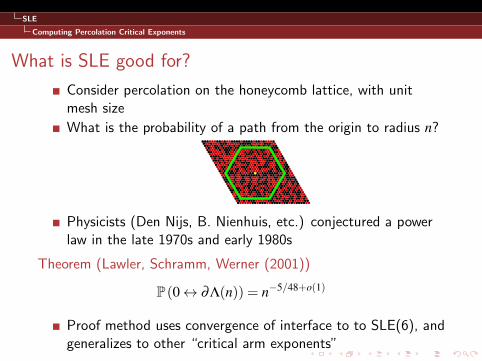
What is SLE good for?
Consider percolation on the honeycomb lattice, with unitmesh size
What is the probability of a path from the origin to radius n?
Physicists (Den Nijs, B. Nienhuis, etc.) conjectured a powerlaw in the late 1970s and early 1980s
Theorem (Lawler, Schramm, Werner (2001))
P(0↔ ∂Λ(n)) = n−5/48+o(1)
Proof method uses convergence of interface to to SLE(6), andgeneralizes to other “critical arm exponents”

SLE
Computing Percolation Critical Exponents
What is SLE good for?
Consider percolation on the honeycomb lattice, with unitmesh size
What is the probability of a path from the origin to radius n?
Physicists (Den Nijs, B. Nienhuis, etc.) conjectured a powerlaw in the late 1970s and early 1980s
Theorem (Lawler, Schramm, Werner (2001))
P(0↔ ∂Λ(n)) = n−5/48+o(1)
Proof method uses convergence of interface to to SLE(6), andgeneralizes to other “critical arm exponents”

CLE
Introduction
What is CLE?
For both percolation and GFF, we had to work to get a singlepath out of the model
More natural questions involve the full model:
Does the collection of all percolation cluster interfaces have alimiting law?Does the zero-set for a zero-boundary-conditions DGFF have alimit?
What about all of the contours?
Zero-height contours of the DGFF on a 300 ⇥ 300 square in Z2.
Jason Miller and Scott She�eld (MSR and MIT) The Gaussian Free Field and CLE(4) February 18, 2011 12 / 34

CLE
Introduction
What is CLE?
For both percolation and GFF, we had to work to get a singlepath out of the model
More natural questions involve the full model:
Does the collection of all percolation cluster interfaces have alimiting law?Does the zero-set for a zero-boundary-conditions DGFF have alimit? What about all of the contours?
Zero-height contours of the DGFF on a 300 ⇥ 300 square in Z2.
Jason Miller and Scott She�eld (MSR and MIT) The Gaussian Free Field and CLE(4) February 18, 2011 12 / 34

CLE
Introduction
What is CLE?
For both percolation and GFF, we had to work to get a singlepath out of the model
More natural questions involve the full model:
Does the collection of all percolation cluster interfaces have alimiting law?
Does the zero-set for a zero-boundary-conditions DGFF have alimit? What about all of the contours?
Zero-height contours of the DGFF on a 300 ⇥ 300 square in Z2.
Jason Miller and Scott She�eld (MSR and MIT) The Gaussian Free Field and CLE(4) February 18, 2011 12 / 34

CLE
Introduction
What is CLE?
For both percolation and GFF, we had to work to get a singlepath out of the model
More natural questions involve the full model:
Does the collection of all percolation cluster interfaces have alimiting law?Does the zero-set for a zero-boundary-conditions DGFF have alimit?
What about all of the contours?
Zero-height contours of the DGFF on a 300 ⇥ 300 square in Z2.
Jason Miller and Scott She�eld (MSR and MIT) The Gaussian Free Field and CLE(4) February 18, 2011 12 / 34

CLE
Introduction
What is CLE?
For both percolation and GFF, we had to work to get a singlepath out of the model
More natural questions involve the full model:
Does the collection of all percolation cluster interfaces have alimiting law?Does the zero-set for a zero-boundary-conditions DGFF have alimit? What about all of the contours?
Zero-height contours of the DGFF on a 300 ⇥ 300 square in Z2.
Jason Miller and Scott She�eld (MSR and MIT) The Gaussian Free Field and CLE(4) February 18, 2011 12 / 34

CLE
Introduction
What is CLE?
CLE(κ) is a random countably infinite collection of loops,each of which “looks like” SLE(κ) locally
No loop of a CLE crosses itself or another loop
Each point in D is almost surely surrounded by infinitely manyloops
For each z ∈ D, let Lk(z) be the kthlargest loop around z.
The sequence Tk(z) =− logCR(Lk(z),z)+ logCR(Lk−1(z),z) isiid with well-understood distribution
∂D
L1(z)
L2(z)
x
density

CLE
Introduction
Exceptional Loop Counts
The conformal radius informationallows us to study the set Φ(θ) ofpoints z for which the numberN(z,ε) of loops surrounding B(z,ε)grows like θ log(1/ε).
∑Nk=1 Tk concentrates around
NET1, so setting NET1 = log(1/ε)tells us that typical behavior isN(z,ε) = 1
ET1log(1/ε)
We can compute the (almost sure)Hausdorff dimension of Φ(θ)
The y-intercept is the dimension ofthe CLE gasket, the set of pointsnot surrounded by a loop
θθ0 ≈ 0.7107
1ET1
dimH(points with θ log(1/ε) loops)
2

CLE
Introduction
Exceptional Loop Counts
Idea for computing dimH(Φ(θ)): arrange disjoint annuli ofradii r1� r2 in the domain
Watch the sequence of loops surrounding the annulus centersuntil a loop hits the inner boundary
Keep only the annuli with loop count approximatelyθ log(r2/r1)
Repeat inside the inner boundary

CLE
Introduction
Exceptional Loop Counts
The probability of having θ log(r2/r1) loops in a given annuluscan be computed using large deviations
Theorem (Cramer)
Suppose (Xi)i∈I are iid and let Λ∗ be the Legendre transform of thelogarithmic moment generating function of the distribution of X1.Then for a < EX1,
P
(1n
n
∑i=1
Xi ≤ a
)= e−nΛ∗(a)+o(1)
Having at least θ log(r2/r1) loops is the same as
∑θ log(r2/r1)k=1 Tk ≤ log(r2/r1)
Substituting into Cramer’s theorem tells us that theprobability of this is (r2/r1)
−θΛ∗(1/θ)+o(1). SodimH(Φ(θ)) = 2−θΛ∗(1/θ)

CLE
Introduction
What is CLE good for?
Can CLE be used to enhance understanding or docomputations?
It is a classical result that for critical percolation, infinitelymany clusters surround the origin
The convergence to CLE gives us some sense of the rate ofgrowth (i.e., logarithmic), via the conformal radius distribution
We can also use CLE to study the continuum Gaussian freefield
, , . . .→ ?

CLE
CLE and the Gaussian free field
The continuum Gaussian free field
The discrete Gaussian free field on {0,ε,2ε,3ε, . . .} (suitablyrescaled) converges to one-dimensional Brownian motion asε → 0
The DGFF on a two-dimensional lattice should converge to ananalogue of Brownian motion with two time dimensions
It turns out that in 2D, it is not possible to define such a limitpointwise
Nevertheless, we can define a limit in the distributional sense
The DGFF h : D→ R can be written as a finite sum ∑i αifi,where αi are iid standard normals and {fi} form anorthonormal basis of the Hilbert space of real-valued functionson D with Dirichlet inner product
(f ,g) = ∑x∼y
(f (x)− f (y))(g(x)−g(y)).

CLE
CLE and the Gaussian free field
The continuum Gaussian free field
The discrete Gaussian free field on {0,ε,2ε,3ε, . . .} (suitablyrescaled) converges to one-dimensional Brownian motion asε → 0The DGFF on a two-dimensional lattice should converge to ananalogue of Brownian motion with two time dimensions
It turns out that in 2D, it is not possible to define such a limitpointwise
Nevertheless, we can define a limit in the distributional sense
The DGFF h : D→ R can be written as a finite sum ∑i αifi,where αi are iid standard normals and {fi} form anorthonormal basis of the Hilbert space of real-valued functionson D with Dirichlet inner product
(f ,g) = ∑x∼y
(f (x)− f (y))(g(x)−g(y)).

CLE
CLE and the Gaussian free field
The continuum Gaussian free field
Similarly, the Gaussian free field is defined via the formal sumh = ∑i αifi, where fi is a fixed orthonormal basis for the Hilbertspace completion of the set of smooth, compactly supportedfunctions on D with inner product
(f ,g) =∫
D(∇f ·∇g) dA
h is not in the Hilbert space, because its L2 norm is infinite
But h is defined as a distribution, since (h,∑i cifi) := ∑i αici
converges almost surely
In particular, h has well-defined circle averages and diskaverages
In fact, (he−t(z))t∈[0,∞) is a Brownian motion, where hr(z) isthe average of h on a circle of radius r centered at z
CLE
CLE and the Gaussian free field
Maxima of the Gaussian free field
What is the extreme behavior of the GFF?
Maxima aren’t defined as such, but we can ask: what is theHausdorff dimension of the set Θ(α) of points z for which
limε→0
avg(h,B(z,ε))log(1/ε)
= α?
Typical behavior corresponds to α = 0, since Bt/t→ 0 almostsurely

CLE
CLE and the Gaussian free field
Maxima of the Gaussian free field
Theorem (Hu, Miller, Peres, 2009)
The Hausdorff dimension of Θ(α) isalmost surely 2−πα2.
Idea of proof: assemble disjointannuli and watch the circle-averageBrownian motions evolve in eachannulus
Some of these will stay pretty closethe line αt
For those that do, repeat in theinner disk
αt

CLE
CLE and the Gaussian free field
GFF via CLE
One may construct the GFF using CLE (Miller & Sheffield)
Sample CLE(4) and flip coins to assign to each loop ±√
π/2
The nth such iterate converges to the GFF in the space ofdistributions as n→ ∞

CLE
CLE and the Gaussian free field
GFF via CLE
One may construct the GFF using CLE (Miller & Sheffield)
Sample CLE(4) and flip coins to assign to each loop ±√
π/2
The nth such iterate converges to the GFF in the space ofdistributions as n→ ∞

CLE
CLE and the Gaussian free field
GFF via CLE
One may construct the GFF using CLE (Miller & Sheffield)
Sample CLE(4) and flip coins to assign to each loop ±√
π/2
−λ +λ
+λ
−λ
−λ
−λ −λ
−λ
+λ
+λ
+λ
The nth such iterate converges to the GFF in the space ofdistributions as n→ ∞

CLE
CLE and the Gaussian free field
GFF via CLE
One may construct the GFF using CLE (Miller & Sheffield)
Sample CLE(4) and flip coins to assign to each loop ±√
π/2
−λ +λ
+λ
−λ
−λ
−λ −λ
−λ
+λ
+λ
+2λ
+2λ0
0+2λ
0
0
0
The nth such iterate converges to the GFF in the space ofdistributions as n→ ∞

CLE
CLE and the Gaussian free field
GFF via CLE
One may construct the GFF using CLE (Miller & Sheffield)
Sample CLE(4) and flip coins to assign to each loop ±√
π/2
+λ
+λ
−λ
−λ
−λ −λ
−λ
+λ
+λ
+2λ
+2λ0
0+2λ
0
0
0
00
0
−2λ
−2λ−2λ
−2λ
The nth such iterate converges to the GFF in the space ofdistributions as n→ ∞

CLE
CLE and the Gaussian free field
Maxima of GFF via CLE
Constructing GFF using CLE paves the way for a CLE-basedtreatment of the GFF maxima
Key idea: finding the points with large ε-disk averagesamounts to finding the points with large sums ∑
Ki=1 ξi, where
ξi =±λ and K is the first index k for which Lk hits the ball ofradius ε.
There is a tradeoff: large K makes it more likely for the sumto be large, but if we ask for K to be too large then we don’tget enough points
(I.e., the sums ∑Ki=1 ξi will have larger K, but there will be
fewer of them and thus there are less likely to be some thatare large)

CLE
CLE and the Gaussian free field
Maxima of GFF via CLE
The optimisation problem is just Cramer’s theorem again
Given α,θ , we can determine the Hausdorff dimension of theset of points surrounded by θ log(1/ε) loops and having GFFdisk average growth α log(1/ε)
We get
P(N ≈ θ log(1/ε),avg≈ α log(1/ε))
≈ P(N ≈ θ log(1/ε))P
(θ log(1/ε)
∑i=1
ξi ≥ α log(1/ε)
)≈ ε
θΛ∗(1/θ)+θΛ∗ξ(α/θ)
This can easily be made precise since Cramer’s theoremguarantees that such exceptional events are highlyconcentrated at the extremes

CLE
CLE and the Gaussian free field
Maxima of GFF via CLE
So for each value of α, there is a unique value of θ thatminimizes θΛ∗(1/θ)+θΛ∗
ξ(α/θ)
This value of θ is the “main contributor” to the set of thepoints having GFF growth rate α log(1/ε)
Recall that the supremum of the growth rates which givenonzero Hausdorff dimension was
√2/π (since the dimension
was 2−πα2.
What loop growth rate corresponds to α =√
2/π?

CLE
CLE and the Gaussian free field
Maxima of GFF via CLE
It turns out that optimum number of loops to get themaximum growth rate of
√2/π log(1/ε) is about 89.5% of
the maximum number of loops.
There is a one-to-one correspondence between these twoportions of the dimension graphs, given byθ = λα/ tanh(π2λα)
θθ0
dimH(points with θ log(1/ε) loops)
2
dimH(points with α log(1/ε) disk averages)
α

CLE
CLE and the Gaussian free field
Maxima of GFF via CLE
It turns out that optimum number of loops to get themaximum growth rate of
√2/π log(1/ε) is about 89.5% of
the maximum number of loops.There is a one-to-one correspondence between these twoportions of the dimension graphs, given byθ = λα/ tanh(π2λα)
θθ0
dimH(points with θ log(1/ε) loops)
2
dimH(points with α log(1/ε) disk averages)
α

CLE
CLE and the Gaussian free field
Thanks!


![Unraveling conformal gravity amplitudesgravity.psu.edu › events › superstring_supergravity › talks › mogull_sstu2018.pdfUnraveling conformal gravity amplitudes based on [1806.05124]](https://img.pdfslide.tips/doc/110x75/5f0cfc827e708231d4381d0d/unraveling-conformal-gravity-a-events-a-superstringsupergravity-a-talks-a.jpg)