Embed Size (px)
Citation preview

Control of DC voltage in Multi-TerminalHVDC Transmission (MTDC) Systems
MOHAMMAD NAZARI
Licentiate Thesis in Electrical EngineeringStockholm, Sweden 2014

TRITA-EE 2014:030ISSN 1563-5146ISBN 978-91-7595-216-1
KTH School of Electrical EngineeringSE-100 44 Stockholm
SWEDEN
Akademisk avhandling som med tillstånd av Kungl Tekniska högskolan framläggestill offentlig granskning för avläggande av teknologie doktorsexamen i datalogiden 29 september 2014 klockan 13.00 i H21, Teknikringen 33, Kungliga Tekniskahögskolan, Stockholm.
© Mohammad Nazari, June 2014
Tryck: Universitetsservice US AB

iii
Abstract
With recent advances in power electronic technology, High-Voltage Di-rect Current (HVDC) transmission system has become an alternative fortransmitting power especially over long distances. Multi-Terminal HVDC(MTDC) systems are proposed as HVDC systems with more than two ter-minals. These systems can be geographically wide. While in AC grids,frequency is a global variable, in MTDC systems, DC voltage can be con-sidered as its dual. However, unlike frequency, DC voltage can not be equalacross the MTDC system. Control of DC voltage in MTDC systemsis oneof the important challenges in MTDC systems. Since the dynamic of MTDCsystem is very fast, DC voltage control methods cannot rely only on remoteinformation. Therefore, they can work based on either localinformation or acombination of local and remote information.
In this thesis, first, the MTDC system is modeled. One of the modelspresented in this thesis considers only the DC grid, and effects of the AC gridsare modeled with DC current sources, while in the other one, the connectionsof the DC grid to the AC grids are also considered.
Next, the proposed methods in the literature for controlling the DC volt-age are described and in addition to these methods, some control methods areproposed to control the DC voltage in MTDC system. These control methodsinclude two groups. The first group (such as Multi-Agent Control methods)uses remote and local information, while the second group (such as SlidingMode Control andH∞ control) uses local information.
The proposed multi-agent control uses local information for immediateresponse, while uses remote information for a better fast response. Applica-tion of Multi-Agent Control systems leads to equal deviation of DC voltagesfrom their reference values. Using remote information leads to better resultscomparing to the case only local information is used. Moreover, the proposedmethods can also work in the absence of remote information.
When AC grid is considered in the modeling, the MTDC system has anon-linear dynamic. Sliding Mode Control, a non-linear control method withhigh disturbance rejection capability, which is non-sensitive to the parametervariations, is applied to the MTDC system. It controls the DCvoltage veryfast and with small or without overshoot.
Afterward, a static state feedbackH∞ control is applied to the systemwhich minimizes the voltage deviation after a disturbance and keeps the in-jected power of the terminals within the limits.
Finally, some case studies are presented and the effectiveness of the pro-posed methods are shown. All simulations have been done in MATLAB andSIMULINK.


Acknowledgment
I want to express my deepest gratitude to my supervisor, Prof. Mehrdad Ghand-hari, for his supervision and feedbacks to my work. Also, I would like to expressmy very great appreciation to Prof. Lennart Söder for being agood support andproviding friendly atmosphere in the department.
The project is financed by the research program Electra whichis deeply ac-knowledged. My deepest respect to the members of my reference group for theircomments on my work: Inger Segerqvist, Kerstin Linden and Magnus Callavikfrom ABB, Magnus Danielsson from Svenska Kraftnät and JonasPersson fromVattenfall. I would like to thank Bertil Berggren for reviewing this thesis and forhis comments.
I would like to thank my friends Amin Ramezanifar, HamidrezaFeyzmahda-vian, Martin Andreasson, Davood Babazadeh and Robert Eriksson for interestingdiscussions we had.
Many thanks to all my colleagues in the department of Electric Power Systems(EPS) for the friendly atmosphere and Fikas!
Last but not least, I want to thank my family who were far away but alwayswith me and I would not have made it this far without them.
v

Contents
Contents vi
1 Introduction 11.1 Background . . . . . . . . . . . . . . . . . . . . . . . . . . . . . 11.2 Multi-Terminal HVDC . . . . . . . . . . . . . . . . . . . . . . . 31.3 DC voltage control strategies . . . . . . . . . . . . . . . . . . . . 51.4 Scope and aim of the project . . . . . . . . . . . . . . . . . . . . 81.5 Contribution . . . . . . . . . . . . . . . . . . . . . . . . . . . . . 91.6 Thesis outline . . . . . . . . . . . . . . . . . . . . . . . . . . . . 10
2 MTDC system modeling 132.1 System modeling . . . . . . . . . . . . . . . . . . . . . . . . . . 13
3 Control strategies 213.1 Introduction . . . . . . . . . . . . . . . . . . . . . . . . . . . . . 213.2 Voltage margin method . . . . . . . . . . . . . . . . . . . . . . . 213.3 Voltage droop method . . . . . . . . . . . . . . . . . . . . . . . . 253.4 Multi-agent control . . . . . . . . . . . . . . . . . . . . . . . . . 273.5 Sliding mode control . . . . . . . . . . . . . . . . . . . . . . . . 353.6 Application to MTDC system . . . . . . . . . . . . . . . . . . . 383.7 H∞ control design . . . . . . . . . . . . . . . . . . . . . . . . . 42
4 Case studies 474.1 Introduction . . . . . . . . . . . . . . . . . . . . . . . . . . . . . 474.2 Study 1 . . . . . . . . . . . . . . . . . . . . . . . . . . . . . . . 494.3 Study 2 . . . . . . . . . . . . . . . . . . . . . . . . . . . . . . . 524.4 Study 3 . . . . . . . . . . . . . . . . . . . . . . . . . . . . . . . 544.5 Comments . . . . . . . . . . . . . . . . . . . . . . . . . . . . . . 56
vi

CONTENTS vii
5 Conclusion and future work 595.1 Conclusion . . . . . . . . . . . . . . . . . . . . . . . . . . . . . 595.2 Future work . . . . . . . . . . . . . . . . . . . . . . . . . . . . . 61
Bibliography 63


List of Acronyms and Symbols
HDVC High-Voltage Direct-CurrentMTDC Multi-Terminal HVDCCSC Current Source ConverterVSC Voltage Source ConverterCPM Constant Power ModeVCM Voltage Control ModeMAS Multi-Agent SystemSMC Sliding Mode ControlSVD Singular Value DecompositionLMI Linear Matrix InequalityVDM Voltage Droop MethodVMM Voltage Margin MethodIGBT Insulated Gate Bipolar TransistorPin j,i Injected active power into DC busiPconv,i Injected active power into converteriPs,i Injected active power at AC busiQconv,i Injected reactive power to converteriQs,i Injected reactive power at AC busiVdc,i Voltage of DC busiIdc,i Injected DC current from DC busi to all buses adjacent to
this busNi Set of all buses adjacent (directly connected) to DC busiVd,i Voltage of terminali projected ond-axisVq,i Voltage of terminali projected onq-axisUd,i Voltage of AC busi projected ond-axisUq,i Voltage of AC busi projected onq-axisIin j,i Injected current by the ideal DC current sourcei
ix


Chapter 1
Introduction
1.1 Background
Thomas Alva Edison invented the first Direct-Current (DC) generator. But, not solong after that, Nikola Tesla and George Westinghouse came up with AlternatingCurrent (AC) idea. AC had an undeniable advantage: its voltage could be changedusing AC transformers. Therefore, the power loss was decreased and it was possi-ble to transmit power over long distances.
After world war II, the need for electric power increased. Insome countrieslike Sweden, the hydro power is located far from the population centers. There-fore, the Swedish engineers in Swedish State Power Board (now Vattenfall) andASEA (now ABB) tried to use DC to transmit power over long distance, but thepower electronic technology could not offer this capability. As a result they uti-lized 380(kV) series-compensated AC lines instead. By advances in power elec-tronic technology, the High-Voltage Direct-Current (HVDC) system became moreclose to be commercial. The first order for an HVDC system was given to ASEAin 1950 to connect the system of the Swedish island of Gotlandto the mainlandsystem. This project was commissioned in 1954.
To choose between AC and HVDC power transmission, a number offactors,both economical and technical must be considered. From economic point of view,HVDC transmission is more expensive than AC transmission. Yet, above a specifictransmission distance, HVDC transmission is cheaper than AC [1, 2]. From tech-nical point of view, HVDC transmission does not need any reactive power on theDC side.
With the advances in power electronic and invention of Insulated Gate Bipolar
1

2 CHAPTER 1. INTRODUCTION
Transistor (IGBT), Voltage-Source Converters (VSC) was introduced and used inthe HVDC systems. The first commercial HVDC based on IGBT was in islandof Gotland in Sweden, which was commissioned in 1997. It was a50(MW) un-derground link from southern part of the island to its northern part [3]. A morecomplete list of VSC-HVDC projects can be found in [4,5].
HVDC systems can be based on Current Source Converter (CSC) or VoltageSource Converter (VSC) or a combination of them. The HVDC systems using theseconverters are called CSC-HVDC and VSC-HVDC, respectively. CSC-HVDC sys-tems are normally used to transmit bulk power over long distances.
VSC-HVDC offers many advantages compared to CSC-HVDC, namely:
• VSC-HVDC does not need an active commutation voltage. The commuta-tion failures resulting from disturbances in AC network will be omitted whenVSC is used.
• VSC offers independent control of active and reactive power, which im-proves the system stability [6]. Also, it makes it possible for VSC-HVDC toprovide the connected AC grids and wind farms with ancillaryservices likereactive power and AC voltage support [2].
• In contrast to CSC-HVDC, it is possible to connect VSC-HVDC to a weaknetwork, because VSCs do not need any reactive power. VSC-HVDC canalso be connected to a "black" network and helps it to black start, providedthat one of the AC grids connected to the VSC-HVDC system operates inthe normal condition [7].
• VSCs have higher PWM frequency which results in very fast dynamic andsmaller filter size [8]. However, this high frequency can increase the switch-ing losses and can also cause Electromagnetic Compatibility (EMC) andElectromagnetic Interference (EMI) issues. On the other hand, multi-levelVSCs are introduced, which have lower switching frequency and a wave-form which is more sinusoidal. As a result, the AC filters willbe smaller orthere is no need to AC filters anymore.
Figure 1.1(a) shows connection of terminali of a VSC-HVDC system to theAC grid i through a phase reactor and a transformer [9]. The filter on the ACside reduces the harmonic entering from the DC side into the AC side. The DCcapacitor is used to keep the DC voltage smooth.

1.2. MULTI-TERMINAL HVDC 3
ACFilter
AC grid VSC DC grid
iV ,dc iVjX
VSC
,dc iV
,Th iZ
iZ
DC grid
iU iV
ACFilter
VSC DC grid
iV ,dc iVjX
,Th iU
(a)
(b)
(c)
Figure 1.1: (a) The positive sequence diagram of terminali connected to AC gridi (b) AC grid is represented by its Thevenin equivalent (c) themodel used in thisthesis.
In this thesis, the AC grid is modeled by its Thevenin equivalent which is avoltage source (UTh,i) behind an impedance (ZTh,i) as shown in Figure 1.1 (b). Nextas seen from the terminali, the AC part is modeled as a voltage source (Ui) withconstant magnitude and phase angle, behind behind an impedance (Zi) as shown inFigure 1.1 (c).
1.2 Multi-Terminal HVDC
Multi-Terminal HVDC (MTDC) systems are HVDC systems consist of more thantwo terminals. The first MTDC system, was build based on CSC technology byadding a 50(MW) converter station at Corsica island to connect Sardinia to themainland Italy HVDC link. This system was commissioned in 1986 [3]. However,in CSC-MTDC systems, in order to change the flow of power, DC voltage polarity

4 CHAPTER 1. INTRODUCTION
must be changed. Since a terminal may be connected to more than one terminal, itproduces undesirable changes in flow of power in other lines.In contrast, in VSC-HVDC system it is possible to change the flow of power without changing thepolarity. Therefore, it is easier to extend the number of terminals in VSC-MTDCsystem, which makes the VSC technology a more attractive solution for MTDCsystems [10,11].
As an example, we consider offshore wind farms. Offshore wind farms maybe one of the main sources of renewable energy in the future. Major offshorewind sources can be far away from the coast. The energy extracted from the windfarms must be transmitted to the shore by means of submarine cables. As statedearlier, VSC-HVDC system can be an attractive solution. Moreover, wind has anintermittent nature, and by interconnecting wind farms to other grids, the effectof intermittency decreases [12]. VSC-MTDC systems make it possible to connectmany of these wind farms together and to the multiple AC gridsand form a DCsystem. On the other hand, there are a lot of oil and gas platforms in the sea. Theseplatforms usually use gas turbines. It would be more efficient if these platforms aresupplied from the offshore grid or wind farms [8]. VSC-MTDC systems make itpossible to build a grid under the sea, which can supply offshore platforms.
VSC-MTDC system in presence of offshore wind farms is studied in differentpapers for example in [13–15]. Figure 1.2 shows an MTDC system connected to3 AC grids and two offshore wind farms and an offshore platform. The systemconfiguration is very similar to the system presented by Airtricity where AC Sys-tem 1 can be considered as UTCE, AC System 2 as the Nordic AC system and ACSystem 3 as the British AC system.
The challenges of operating MTDC systems, like controllingthe DC volt-age, power flow in DC lines, interaction between converters,have been discussedin [16]. One of the most important issues is that the DC voltage across the MTDCsystem must be kept in an acceptable range. DC over-voltage could damage theconverters, whereas DC under-voltage may result in reducing the converter con-trollability [17]. If the power balance in the MTDC system isnot maintained, theDC voltage will change. VSC operating in rectifying mode injects active powerto the MTDC system, while the VSC operating in inverting modeextract activepower from it. If more active power is injected into the DC grid, the DC voltagewill increase. An analogy for the DC voltage control in a 5-terminal MTDC systemis presented in Figure 1.3. Each converter is replaced by an avatar and the heightof the balls from the earth resembles the voltage of terminals. These avatars try tokeep the height of the grid in the acceptable area, which is identified bymaxandmin.

1.3. DC VOLTAGE CONTROL STRATEGIES 5
AC
grid1
AC
grid2
AC grid3
DC gridVSC
VSC
VSC
VSC
VSCVSC
Offshore
wind farm
MTDC
system
VSC
AC terminal
DC bus
Offshore
wind farm
Offshore
platform
VSC VSC
Figure 1.2: A VSC-MTDC system.
Figure 1.3: An analogy for a 5-terminal MTDC system.
1.3 DC voltage control strategies
To control the DC voltage of the converters, remote information may be useful asinput data. However, since the dynamic of the VSC-MTDC system is very fast,we may not only rely on remote information, especially during disturbances orjust after a disturbance. Therefore, any proposed control algorithm should rely oneither local data or on a combination of local and remote data. In the power systemliterature, different DC voltage control methods have beenproposed. Among them,Voltage Margin Method (VMM) and Voltage Droop Method (VDM) are the mostwell-known methods. These two methods rely on local information as input datato control the DC voltage of the converters. Ref. [18] reviews VMM and different

6 CHAPTER 1. INTRODUCTION
types of VDM strategies. Some authors [19,20] proposed control strategies, whichare a combination of VDM and VMM.
In VDM, all or some converters participate in the DC voltage control by chang-ing their injected active powers (or DC currents) based on a predefined droop. Ap-plication of this method results in a steady-state DC voltage deviation from thepre-disturbance values. In contrast, in VMM one converter (slack converter) isresponsible to maintain its DC voltage in the desired level,while other terminalsoperate at constant power mode [21]. Due to some technical constraints, when theDC voltage controller converter is not any longer able to supply or extract the ac-tive power necessary for controlling its DC voltage, another converter will operateas the slack converter [22]. A margin must be considered between the referenceDC voltages of terminals. The transition between these two reference voltages putsa lot of stress on the converter [23]. Moreover, the voltage margin must be consid-ered large enough in order to avoid interactions between controllers [22]. VMMmay be single stage or multi-stage. Different types of VMM inpresence of off-shore windfarms and also a discussion on prioritizing converters in controlling DCvoltage is presented in [24].
Ref. [25] implements the droop control for a VSC-MTDC system. In this refer-ence, VDM is used, and the droops are determined using LinearMatrix Inequality(LMI) to minimize the voltage deviation, and only the DC dynamics are consid-ered. Authors of [8], modeled the VSC-MTDC system as a Multi-Input Multi-Output (MIMO) system. Then, the different values of droops of the controllershave been analysed in this paper using Singular Value Decomposition (SVD).
Ref. [26] uses an adaptive method for calculating this droop. After each con-tingency, converters work at new operating points. The aim is that, converters withmore headroom available for the power, should participate more in the DC voltagecontrol.
Ref. [27] implements a variable droop method. In the proposed method in thisstudy, the droop is changed according to the injected power of the converter tominimize the loss in the DC grid. On the other hand, this change in the injectedactive power of the converters may be considered as a disturbance from the ACgrid point of view. This can have an impact on the AC grid stability. This issue isstudied in paper [28].
VSC-MTDC system can control the frequency in the connected AC grids. Iffrequency drops in an AC grid, the VSC-MTDC system injects more active powerto (or extract less active power from) the AC grid. This reflects on the DC voltage,and since in VDM different terminals participate in DC voltage control, other ACgrids will be affected by this change. This issue is discussed in [29].

1.3. DC VOLTAGE CONTROL STRATEGIES 7
Ref. [30,31] studied the power flow when VDM is applied to the VSC-MTDCsystem. The different power sharing in converters using VDMis discussed in [32].
The stability of VSC-MTDC system in general and also in the presence ofoffshore wind farms is discussed in [6,33,34].
Multi-agent system
Multi-Agent System (MAS) is an application of distributed intelligence, whichbrings intelligence on a component level [35]. An agent is a software entity, whichis situated within an environment and can act autonomously in response to the en-vironment changes [36, 37]. A multi-agent system is a systemcomprising two ormore agents. It should be noted that there is no global goal inthe multi-agent sys-tem. Each agent has its own goal and changes its behavior dynamically to achieveits own goal. Agents may or may not communicate with each other.
MAS is used for different aims in the literature. Ref. [36,38] reviewed some ap-plications of MAS to power systems. Some authors [35, 39–41]studied the powersystem restoration using MAS. Secondary control of power system in presence ofFACTS devices is another application of MAS, which is studied in [42,43].
In this thesis, the proposed MAS control methods use both local and remoteinformation to control the DC voltage and make the DC voltagedeviation of the DCbuses equal. MAS can use different strategies like incremental strategy, consensusstrategy and diffusion strategy. The consensus strategy isused in this thesis.
Sliding mode control
Sliding Mode Control (SMC) is a variable structure control,which is originallyused for systems whose dynamics can be modelled with ordinary differential equa-tions. SMC has some features like insensitivity to parameter variations, externaldisturbance rejection and fast dynamic response [44, 45]. In this method, the ideais to define a surface along which the tracking error is zero. The controller forcesthe system to slide along this surface. One of the common problems of SMC ischattering around this sliding surface.
SMC is used for power oscillation damping in [46]. In [47] SMCis applied toa 2-terminal HVDC system. However, SMC has not been applied to the MTDCsystem. In this thesis, a control method based on SMC for MTDCsystem is pre-sented. Based on this method, one converter controls the DC voltage, while otherconverters operate in constant power mode.

8 CHAPTER 1. INTRODUCTION
H∞ control
In theH∞ control design method, a feedback controller is sought to stabilize theclosed-loop system and satisfy a prescribed level of performance. In this method,the control problem is expressed as a mathematical optimization problem. The de-sired performance requirements will be expressed as constraints of this optimiza-tion problem. In this method, the controller tries to minimize the maximum of thetransfer function of the desired of the desired signal all over the time. This leads tosolving a Linear Matrix Inequality (LMI).
Ref. [48] applies theH∞ to control the DC voltage in HVDC system which isinstalled in parallel with an AC line. Also in [49] anH∞ control is designed toenhance the stability of the VSC-HVDC system. In this thesis, a static-feedbackH∞ is applied to MTDC system with injection model. The purpose of this con-troller is to minimize the deviation of the DC voltage of the MTDC system, after adisturbance. Meanwhile, it limits the powers injected fromthe AC grids and alsoprevents the congestion in some of the DC lines. Moreover, the converters par-ticipate in voltage control, based on their available capacity. In this method, likeVDM, some or all converters participate in voltage control.
1.4 Scope and aim of the project
As mentioned before, one of the important challenges in MTDCsystems is to con-trol the DC voltage and to keep secure operation of the VSC-MTDC system innormal conditions and after each contingency in the system.Another challenge isto find the optimal injected active powers of converters before and after the contin-gency, which is beyond the scope of this thesis. Also, the stability and oscillationsof the AC grids are not studied in this thesis. This issues will be studied in the nextphase of this project.
The aim of this thesis is to develop new control methods for controlling theDC voltage in VSC-MTDC system. To achieve this aim, first the MTDC systemis modeled using two approaches. In the first approach, only the dynamic of theDC grid is considered and AC grids are modeled with DC currentsources. In thesecond approach, both AC grid and DC grid are modeled. The AC grid is modeledby its Thevenin equivalent. TheH∞ control is applied on the first model, while thesliding mode control is applied on the second model. Other control methods areapplied using both models . In this thesis the fast dynamics due to the inductancesof the DC lines have not been considered. Also, it is supposedthat the AC gridsare not connected to each other.

1.5. CONTRIBUTION 9
Next, the control methods proposed in the literature for controlling the DCvoltage are presented and their advantages and disadvantages are described. Sincein controlling the DC voltage both local information and a combination of localand remote information can be used, the methods presented inthis paper can bedivided in two groups. The first group, including Multi-Agent Control methods,use remote and local information, while the second group (Sliding Mode ControlandH∞ control), use local information.
This work will be later developed to consider the more detailed model of ACgrids, the economic aspects of using MTDC systems and optimal injected powers.
1.5 Contribution
This thesis addresses different aspects of control of VSC-MTDC system. In thisregard, the following contributions are listed:
• The future MTDC systems may be geographically wide with longdistancesbetween the converters. Therefore, a distributed and intelligent control method-ology may be needed to operate such systems. This thesis aimsto proposeDC voltage control algorithms based on MAS. These methods may rely oneither local information or a combination of local and remote data. First pro-posed control method has a smaller steady-state error comparing to VDM.
• Another MAS-based control method is proposed. In this method, the systemtries to minimize the voltage deviation after a disturbanceand at the sametime, terminals participate exactly proportional to theirdroop.
• A sliding-mode control for VSC-MTDC system is proposed in this thesis.This method is robust, fast, insensitive to parameter variations and distur-bances. It works based on local information.
• An H∞ controller is proposed for control of DC voltage in MTDC systems.Using this controller, the deviation of DC voltage will be minimized and theinjected active power of converters will be kept within the limits.
List of publications
•C1 Mohammad Nazari and Mehrdad Ghandhari, "Application of multi-agentcontrol to multi-terminal HVDC systems", IEEE EPEC Conference (Canada),

10 CHAPTER 1. INTRODUCTION
2013. Mohammad Nazari carried out the work and wrote the paper under su-pervision of Mehrdad Ghandhari.
• C2 Martin Andreasson, Mohammad Nazari, Dimos Dimarogonas, Henrik Sand-berg, Karl H.Johansson and Mehrdad Ghandhari, "Distributed Voltage andcurrent control of VSC multi-terminal high voltage direct current transmis-sion systems", Accepted in IFAC 2014 conference. This paperwas resultof collaboration between Electric Power System and Automatic Control de-partments. Mohamamd Nazari and Martin andreasson carried out the workand wrote the paper under supervision of other authors.
• C3 Mohammad Nazari, Mehrdad Ghandhari, "H∞ control of Multi-TerminalHVDC systems", CIGRE AORC conference, 2014. Mohammad Nazari car-ried out the work and wrote the paper under supervision of Mehrdad Ghand-hari.
• J1 Mohammad Nazari, Mehrdad Ghandhari, Amin Ramezanifar, "Sliding-modecontrol of Multi-Terminal HVDC transmission system", Submitted to IEEETransactions on Power Delivery. Mohammad Nazari carried out the workand wrote the paper under supervision of Mehrdad Ghandhari.He used thecomments of Amin Ramezanifar.
Table 1.1: Table of the methods used in papers
VDM VMM MAS SMC H∞C1 X X
C2 X X
C3 X X
J1 X X
1.6 Thesis outline
The outline of this thesis is as follows
• Chapter 2 gives the technical background related to modeling of VSC-MTDCsystem. Two main modeling approaches are considered in thischapter, namely:
1.6. THESIS OUTLINE 11
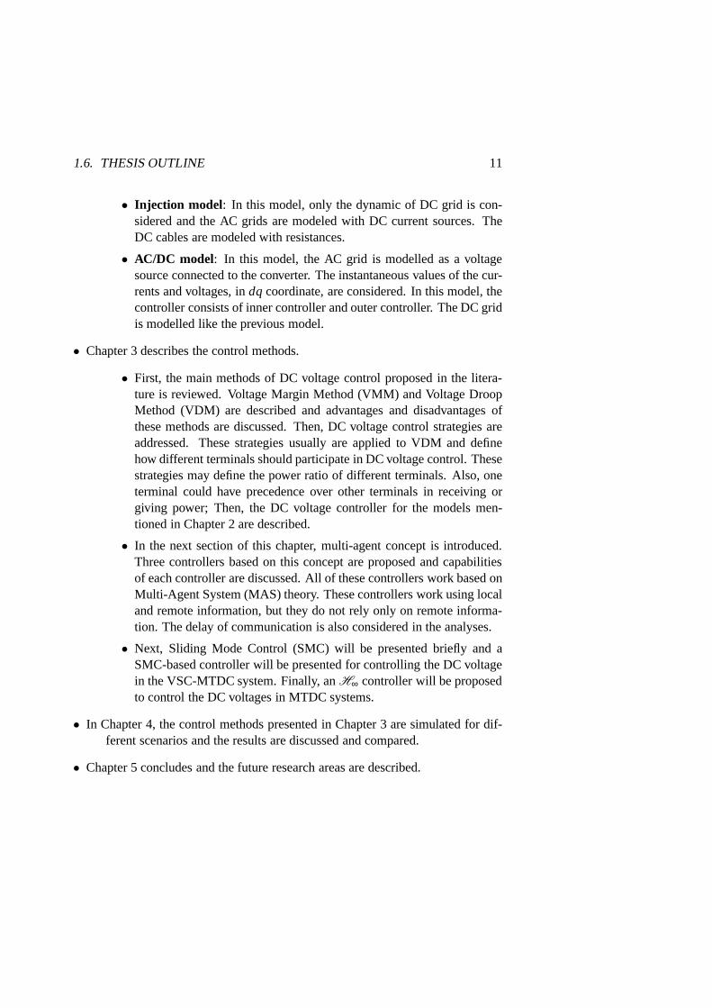
• Injection model: In this model, only the dynamic of DC grid is con-sidered and the AC grids are modeled with DC current sources.TheDC cables are modeled with resistances.
• AC/DC model: In this model, the AC grid is modelled as a voltagesource connected to the converter. The instantaneous values of the cur-rents and voltages, indq coordinate, are considered. In this model, thecontroller consists of inner controller and outer controller. The DC gridis modelled like the previous model.
• Chapter 3 describes the control methods.
• First, the main methods of DC voltage control proposed in thelitera-ture is reviewed. Voltage Margin Method (VMM) and Voltage DroopMethod (VDM) are described and advantages and disadvantages ofthese methods are discussed. Then, DC voltage control strategies areaddressed. These strategies usually are applied to VDM and definehow different terminals should participate in DC voltage control. Thesestrategies may define the power ratio of different terminals. Also, oneterminal could have precedence over other terminals in receiving orgiving power; Then, the DC voltage controller for the modelsmen-tioned in Chapter 2 are described.
• In the next section of this chapter, multi-agent concept is introduced.Three controllers based on this concept are proposed and capabilitiesof each controller are discussed. All of these controllers work based onMulti-Agent System (MAS) theory. These controllers work using localand remote information, but they do not rely only on remote informa-tion. The delay of communication is also considered in the analyses.
• Next, Sliding Mode Control (SMC) will be presented briefly and aSMC-based controller will be presented for controlling theDC voltagein the VSC-MTDC system. Finally, anH∞ controller will be proposedto control the DC voltages in MTDC systems.
• In Chapter 4, the control methods presented in Chapter 3 are simulated for dif-ferent scenarios and the results are discussed and compared.
• Chapter 5 concludes and the future research areas are described.


Chapter 2
MTDC system modeling
2.1 System modeling
Consider again Figure 1.1 (a). As mentioned in chapter 1, a VSC-MTDC systemconsists of DC Cables, converters, filters and DC capacitors. Different approachesfor modeling MTDC system have been proposed in the literature [10,50].
Depending on the purpose of the study, DC cables can be modeled with dis-tributed model [33] or withπ-circuit model [23]. The distributed model is suitablefor transient analysis, while theπ-circuit model is utilized for slower dynamics.For applying the proposed control methodologies in this thesis, theπ-circuit modelis chosen and the fast dynamic due to the inductances of the DCcables and theswitchings of the converters are not considered in this study. The shunt DC ca-pacitor installed in each DC bus is also included in the capacitor of the π-circuitmodel.
Converters are responsible for injecting active power to MTDC system or ex-tracting power from it. Different modeling approaches are presented in the litera-ture. Two models have been used for the purpose of this thesis. In the first model,only the dynamic of the DC grid is considered and the power exchange betweenAC and DC are represented by DC current sources. In the secondmodel, the ACgrids are modeled as voltage sources connected to the converters. In this model,the instantaneous values of currents and voltages, indq reference frame, are con-sidered [10].
13

14 CHAPTER 2. MTDC SYSTEM MODELING
Model 1: Injection model
Figure 2.1 illustrates an asymmetric monopole MTDC system with ground return,and with n DC buses. These buses (1 ton) are connected to the AC terminalsthrough converters. The AC terminals are connected to AC grids 1 ton. Sincethe interactions between the AC grids and the MTDC system arerepresented bycurrent sources, the AC terminals are not shown in this figure.
Other DC buses (n+1 tom), called DC hubs, are the junctions between the DCcables. However, in this thesis, we suppose that there is no DC hub in the MTDCsystem, and as a resultm= n.
DC grid:
DC cables are
modelled with
resistors
,dc nV
,1dcV
,1dcI
,ndcI
inj,1I
inj,nI
1C
nC
Figure 2.1: An n-terminal MTDC grid. Converters are modeledas DC currentsources.
In this figure,Ci is the aggregated capacitance of the DC cables connected tothe converteri and the DC capacitor of the converteri, Vdc,i is the DC voltage ofthe DC bus of the converteri. The active power exchange between the AC gridiand the MTDC system is represented by DC current source indicated byIin j,i . Theinjected active power is defined as follows
Pin j,i =Vdc,i × Iin j,i (2.1)

2.1. SYSTEM MODELING 15
In this thesis, a positivePin j,i means active power is injected from the AC gridi into the MTDC system, while a negativePin j,i means active power is extractedfrom the MTDC system. Thus, the dynamic of the converteri, which is connectedto the AC gridi, is described by (fori = 1. . .n)
Vdc,i =1Ci
(Iin j,i − Idc,i) (2.2)
whereIdc,i is the DC current from busi to the adjacent buses, and it is expressed by
Idc,i = ∑j∈Ni
gi j (Vdc,i −Vdc, j ) (2.3)
In equation (2.3),Ni is the set of adjacent buses to busi, gi j =1
Ri j, andRi j represents
the resistance of the cable between the terminalsi and j.Thus, the dynamic of then-terminal MTDC system can be described by a set
of differential equations of the form
xDC = ADCxDC+BDCuDC (2.4)
where,
xDC =
Vdc,1...
Vdc,n
, uDC =
Iin j,1...˙Iin j,n
(2.5)
and
A =
− 1C1
∑j∈N1
g1 j . . . g1nC1
.... . .
...gn1Cn
. . . − 1Cn
∑j∈Nn
gn j
(2.6)
B =
1C1
0 . . . 00 1
C2. . . 0
......
. . . 00 0 . . . 1
Cn
(2.7)
16 CHAPTER 2. MTDC SYSTEM MODELING
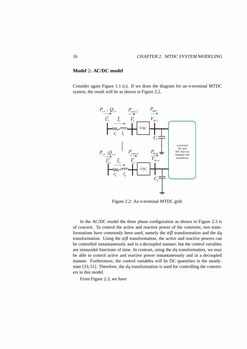
Model 2: AC/DC model
Consider again Figure 1.1 (c). If we draw the diagram for ann-terminal MTDCsystem, the result will be as shown in Figure 2.2.
VSC
inj,1P
inj,nP
n-terminal
DC grid
(DC lines are
modeled with
resistances)
,1convP
,nconvP
,1 ,1,s sP Q
, ,,s n s nP Q
1r
nr
1l
nlVSC
nU
1U
1V
nV
,dc nV
,1dcV
1I
nI
1C
nC
Figure 2.2: An n-terminal MTDC grid.
In the AC/DC model the three phase configuration as shown in Figure 2.3 isof concern. To control the active and reactive power of the converter, two trans-formations have commonly been used, namely theαβ transformation and thedqtransformation. Using theαβ transformation, the active and reactive powers canbe controlled instantaneously and in a decoupled manner, but the control variablesare sinusoidal functions of time. In contrast, using thedq transformation, we maybe able to control active and reactive power instantaneously and in a decoupledmanner. Furthermore, the control variables will be DC quantities in the steady-state [33,51]. Therefore, thedq transformation is used for controlling the convert-ers in this model.
From Figure 2.3, we have

2.1. SYSTEM MODELING 17
Averaged ideal
three-phased
VSC
,a iv
,b iv
,c iv
,a iu
,b iu
,c iu
il ir
DC grid
Figure 2.3: The three phase model of AC gridi connected to the converteri.
ua,i −va,i = l idia,idt
+ r i ia,i
ub,i −vb,i = l idib,idt
+ r i ib,i
uc,i −vc,i = l idic,idt
+ r i ic,i
(2.8)
These equations are transformed to thedq reference frame [10], and the followingare obtained
[Ud,i
Uq,i
]−
[Vd,i
Vq,i
]=
[r i −ωi l i
ωi l i r i
][Id,iIq,i
]+
[l i 00 l i
]ddt
[Id,iIq,i
](2.9)
whereId,i andIq,i are thed andq components of the current flowing from AC gridto the converter,Ud,i andUq,i , are thed andq components of the voltage source ofthe AC gridi which are assumed constant, and finallyVd,i andVq,i are thed andqcomponents of the AC terminali.
Thus, the dynamic of the terminali is described by a set of differential equa-tions of the form (fori = 1. . .n)
Id,i =−r iId,i
l i+ωi Iq,i +
Ud,i
l i−
Vd,i
l i(2.10)
Iq,i =−r i Iq,i
l i−ωiId,i +
Uq,i
l i−
Vq,i
l i(2.11)

18 CHAPTER 2. MTDC SYSTEM MODELING
The equations of the terminali can be written in a general form as
xAC,i = fAC,i(xAC,i)+BAC,iui (2.12)
where
xAC,i =
[Id,iIq,i
],ui =
[Vd,i
Vq,i
](2.13)
fAC,i(xAC,i) =
[f1,if2,i
]=
[−r i Id,i
li+ωi Iq,i +
Ud,i
li−r i Iq,i
li−ωiId,i +
Uq,i
li
](2.14)
BAC,i =
[− 1
li0
0 − 1li
](2.15)
To complete the dynamical model, the DC part of the system must also be consid-ered. From Figure 2.2, the link between the AC and DC parts of terminali can beexpressed by
Vdc,i =Pin j,i
Vdc,iCi−
Idc,i
Ci(2.16)
whereIdc,i is given in (2.3).Therefore the dynamic of terminali can be expressed as
xi = f i(xi)+biui (2.17)
where
xi =
[xAC,i
xDC,i
]=
Id,iIq,i
Vdc,i
(2.18)
f i(xi) =
f1,if2,if3,i
=
−r i Id,ili
+ωi Iq,i +Ud,i
li−r i Iq,i
li+ωiId,i +
Uq,i
liPin j,i
Vdc,iCi− 1
Ci∑
j∈Ni
gi j (Vdc,i −Vdc, j )
(2.19)

2.1. SYSTEM MODELING 19
In Figure 2.2, the active power exchange with AC gridi is expressed by
Ps,i =Ud,i Id,i +Uq,iIq,i (2.20)
and the power received by the converteri is
Pconv,i =Ud,i Id,i +Uq,iIq,i − r i(I2d,i + I2
q,i) (2.21)
Since the converter is considered to be lossless, we have
Pin j,i = Pconv,i (2.22)
Next, based on Figure 2.2, the reactive power exchange with AC grid i can beexpressed as
Qs,i =Uq,i Id,i −Ud,i Iq,i (2.23)
Using Phase-Locked Loop (PLL), thed axis of thedq reference frame will bealigned with thea-phase of theabcreference frame. Supposing that the PLL track-ing is perfect, it results inUq,i = 0, and equations (2.20) and (2.23) can be writtenas, [51],
Ps,i = Ud,i Id,i (2.24)
Qs,i = − Ud,i Iq,i (2.25)
Thus,Ps,i is controlled byId,i andQs,i is controlled byIq,i .

Chapter 3
Control strategies
3.1 Introduction
Different control strategies have been proposed in the literature. Voltage Mar-gin Method (VMM) and Voltage Droop Method (VDM) are the two most well-known methods. These methods do not need any communication between termi-nals. However, as mentioned in Section 1.3, each of these methods has some disad-vantages. In this section, we first explain voltage margin method and voltage droopmethod. Then, some new methods based on Multi-Agent Systems(MAS) and Slid-ing Mode Control (SMC) are proposed to enhance the VMM and VDM. The MASmethods require communication between terminals to achieve their goals, how-ever, they can still work without communication. SMC controller proposed in thisthesis is a modification of VMM and does not need any communication betweenterminals.
3.2 Voltage margin method
In VMM one converter is responsible to maintain the DC voltage of the MTDCsystem on a desired level, while other converters operate atConstant Power Mode(CPM) [21]. If the converter on DC Voltage Control Mode (VCM)is no longer ableto supply or extract the required power to control the DC voltage, the DC voltagechanges, and when the voltage reaches reference value of an another converter,then the corresponding converter will operate as slack converter [22].
Figure 3.1 shows the characteristics of VMM for a two-terminal HVDC sys-tem. A margin must be considered between two control voltagelevels [21]. If
21

22 CHAPTER 3. CONTROL STRATEGIES
the voltage margin is not large enough, it is possible that, in transients, more thanone converter participate in the DC voltage control and thiscauses the interactionbetween converters [22]. In this figure, the operating pointis marked with a redpoint. As can be seen, converter 2 is operating in VCM and keepthe DC voltageat its reference value (V re f
dc,2) and terminal 1 is operating in CPM. Recalling that, inthis thesis, a positive injected power represents the powerinjected to the MTDCsystem, it can be concluded that converter 1 is operating as inverter and converter2 is operating as rectifier. Therefore, the flow of the power isfrom DC bus 2 to DCbus 1.
Voltage Control
Mode
Inverter Rectifier
Terminal 1
Terminal 2
voltage margin
current operating
point
Constant Power
Mode
dcV
injP max
injP min
injP
Figure 3.1: VMM control strategy characteristics.
Two methods are proposed in the literature to change the direction of powerflow. In the first method, the reference power of converter 1 ischanged (Figure3.2(a)), and in the second method, the reference voltage of converter 2 is changed,which is shown in Figure 3.2(b). In the latter, both characteristics cross the verticalaxis. As a result, if one converter stops working, the other one can work atPin j =0. In other words it can supply the reactive power, i.e. working as a STATicsynchronous COMpensator (STATCOM) [22].
As it can be seen in Figure 3.1, if converter 1 reaches its limits or stops oper-ating, converter 2 is responsible for control of DC voltage.However, if converter1 reaches its limit and converter 2 cannot control the DC voltage, the DC voltagewill be out of control [52]. Considering the delays in communication [53], someauthors proposed a VMM controller with two stages [21, 52], whoseVdc−Pin j
characteristic is shown in Figure 3.3.

3.2. VOLTAGE MARGIN METHOD 23
Terminal 1
Terminal 2
dcV
injP
(a)
Terminal 1
Terminal 2
dcV
injP
(b)
Figure 3.2: Direction change of power flow: (a) by changing reference power ofterminal 1, (b) by changing reference voltage of terminal 2.
lower stage
upper stage
,
up
dc iV
,
low
dc iV
,dc iV
,inj iP
max,low
,inj iP min,up
,inj iP min,low max,up
, , ,
ref
inj i inj i inj iP P P= =
Terminal 2
Terminal 1
Figure 3.3: VMM applied to a two-terminal HVDC system. Converter 1 has atwo-stage VMM controller, while converter 2 has ordinary VMM controller.
In this strategy, there are two constant voltage levels. Each of these levels hasa maximum and minimum allowable injected power. If the injected power of theconverter reaches these values, it switches to CPM. If the voltage changes againand reaches to one of these constant voltage levels, it switches again to the VCM.The two-stage characteristic has two other advantages. First, the active power inall terminals can be set by changingPre f . Second, it would be possible to assigna certain amount of importance to each terminal; for example, if one converteris connected to a very strong AC grid which can produce as muchactive power

24 CHAPTER 3. CONTROL STRATEGIES
as needed, thenPmin andPmax can be chosen far from each other. Therefore, thisconverter can operate as the slack in the system [22].
Since VSCs can operate both as rectifier and inverter, [52] suggests that anotherstage, can also be added to the converter control characteristics. In this thesis,ordinary (single-level) VMM is considered. Figure 3.4 shows the block diagramof VMM controller for converteri when the injection model is used. As shown in
, ,dc ref iV
,dc iV
0,inj iP
,inj iPD
,
set
inj iPD
å+
-
å+
+
¸
,dc iV
,inj iP
max
inj, iP
min
,inj iP
Sw1
Sw2
,
,
I i
p i
KK
S+
,inj iI
Figure 3.4: VMM controller for converteri when the injection model is used.
the figure, a Proportional-Integral (PI) controller is used. If the injected power hitsone of the limits (Pmax
in j,i or Pminin j,i), terminali switches to CPM. If AC/DC model is
used, the controller is implemented as shown in Figure 3.5. The controller givesthe reference values of thed-axis andq-axis currents to the inner controller.
,
ref
dc iV
,dc iV 0
,d iI
å+
-å
+
+
,
ref
d iID
,
ref
d iI
,
ref
inj iP
0
,d iI
å+
-å
+
+
,
ref
d iID2,i
2,
I
P i
KK
s+
,inj iP
,
ref
ac iV
,ac iV 0
,q iI
å+
-å
+
+
,
ref
q iID
,
ref
inj iQ
å+
-å
+
+
4,i
4,
I
P i
KK
s+
,inj iQ
,
ref
q iID
Sw1
Sw2
0
,q iI
,
ref
q iI
3,i
3,
I
P i
KK
s+
Sw3
Sw4
1,i
1,
I
P i
KK
s+
Figure 3.5: VMM controller for terminali when the AC/DC model is used.

3.3. VOLTAGE DROOP METHOD 25
3.3 Voltage droop method
Another proposed method in the literature is Voltage Droop Method (VDM) [22,54, 55]. If more than one converter are supposed to participate in the DC voltagecontrol, VDM is a reliable method, which does not need any communication be-tween converters [11, 56, 57]. In this method some or all converters change theirinjected active powers according to pre-definedVdc−Pin j droops [22]. Figure 3.6shows this characteristic.
Terminal 2
Terminal 11OP
2OP
max
,1invP max
,1recP
injP
dcV
,1injP
,2injP
Figure 3.6: VDM control strategy characteristics for a two-terminal HVDC system.
As can be seen, converters 1 and 2 are operating atOP1 andOP2, respectively.It must be noted that in this figure, for convenience, it is supposed that the voltagesof DC buses are equal. However, this is not the case in reality.
It must be stated that, some authors [23,31,58] useVdc−Pin j characteristic forvoltage droop control, whereas others [17,25,57] studiedVdc− Iin j characteristic.
DC voltage droop control has some disadvantages. Considering the type of thesystem, application of VDM leads to steady-state voltage deviation. The controlleradjusts power according to this voltage deviation. Considering that the voltagedeviation is not equal in all DC buses (especially when busesare located veryfar from each other and as a result the DC resistance is large), the power is notshared proportional to the droops of converters. Moreover,if the network topologychanges, the droop characteristic is not valid anymore [52].
Employing high droop gain leads to large DC voltage deviation. On the otherhand, AC gridi considers the changes in thePin j,i as a disturbance and low droopgain results in large disturbance from the corresponding ACgrid point of view.
Figures 3.7 and 3.8 represent the block diagram of the VDM controller wheninjection model and AC/DC model is used, respectively.

26 CHAPTER 3. CONTROL STRATEGIES
, ,dc ref iV
,dc iV 0,inj iP
,inj iPDå
+
-å
+
+
¸
,dc iV
,inj iP
max
inj, iP
min
,inj iP
,p iK,inj iI
Figure 3.7: VDM controller for converteri when the injection model is used.
,
ref
dc iV
,dc iV 0
,d iI
å+
-å
+
+
1,P iK,
ref
d iID
,
ref
d iI
,
ref
inj iP
0
,d iI
å+
-å
+
+
,
ref
d iID2,i
2,
I
P i
KK
s+
,inj iP
,
ref
ac iV
,ac iV 0
,q iI
å+
-å
+
+
,
ref
q iID
,
ref
inj iQ
å+
-å
+
+
4,i
4,
I
P i
KK
s+
,inj iQ
,
ref
q iID
Sw1
Sw2
0
,q iI
,
ref
q iI
3,i
3,
I
P i
KK
s+
Sw3
Sw4
Figure 3.8: VDM controller for converteri when the AC/DC model is used.
Comparing Figures 3.5 and 3.8, it is evident that only DC voltage controllersare different in these two methods. While VMM uses a PI controller, VDM utilizesa proportional controller.
The VDM used in this thesis is ordinary (proportional) VDM. However, someauthors propose another schemes for VDM [18]. As an example,we mention thepriority power sharing VDM. In the systems with priority power sharing, someterminals have precedence over others in receiving or giving power. For instance,as shown in Figure 3.9, converter 2 does not participate in DCvoltage control. Ifthe voltage increases and reachesVmin
dc,2, converter 2 starts to extract active powerfrom the MTDC system and controls the DC voltage.

3.4. MULTI-AGENT CONTROL 27
Terminal 1
Terminal 2
min
,2dcV
injP
dcV
Figure 3.9: Priority VDM control strategy characteristic for a two-terminal HVDCsystem.
3.4 Multi-agent control
Mathematical background
Since Multi-Agent Systems (MAS) utilize graph theory, in this section a very shortintroduction to graph theory is given.
Consider a graphG= {V,ε} consisting of a set of vertices (nodes)V = {1, ...,N}and edgesε , as shown in Figure 3.10, where
ai j =
{1 if nodesi and j are adjacent
0 otherwise(3.1)
If there is a link or edge between two nodesi and j , they are called adjacentnodes i.e.,ε = {(i, j) ∈V×V : i, j adjacent}. A graph is called ’connected’ if thereis a path connecting each two nodes together. The distance between two nodes isthe shortest path with minimum number of edges that connectsthose nodes and isshown byd(i, j). The degree matrixD with the elements ofdi is a diagonal matrixwhose elements are the cardinality of agenti neighbor setNi = { j ∈ v : (i, j) ∈ ε}.
Figure 3.10 shows an information graph. As can be seen,N1 consists of nodes2, 3 and 6. A tree is defined as a undirected graph in which any two nodes are

28 CHAPTER 3. CONTROL STRATEGIES
4 5
3 2
1
6
1N
12
21
a
a=
12ε
13ε
16ε
Figure 3.10: Information graphG.
connected by only one simple path. A spanning three is a tree which consists ofall nodes of a graph. One of the most important matrices in graph theory, whichreflects significant characteristics of the graph isLaplacian matrix. The i j − thelement of the Laplacian matrixL is determined as
l i j =
n∑
k=1k6=i
aik j = i
−ai j j 6= i
(3.2)
Considering undirected graph as shown in Figure 3.10, the Laplacian matrixis symmetric and positive semi-definite in which the sum of the elements in eachrow is zero. Therefore,L has a zero eigenvalue, i.e.λ1 = 0. The second smallesteigenvalue (λ2) is called connectivity of the graph. In a connected undirected graphwe have [59]:
0= λ1 < λ2 ≤ . . .≤ λn (3.3)
Consider a graph, in which each nodei has the following control law:
ui = ∑j∈Ni
−ai j (xi −x j) (3.4)
whereui is the control input andxi is state variable. We say nodes of the networkreach aconsensusif and only if xi = x j = . . . = xn = x⋆. Then, the dynamic of the

3.4. MULTI-AGENT CONTROL 29
system can be written as
x(t) =−LLL x(t) (3.5)
Since eigenvalues ofLLL are positive, eigenvalues of−LLL are in Left-Hand Plan(LHP). Therefore the system is stable. One can show that the nodes of the undi-rectional graph reaches consensus if and only of there is a spanning tree in thegraph [60].
Application to MTDC system
Consider an MTDC system consisting of several converters. Each terminal is con-sidered as a node in the graph. Some terminals like the ones connected to windfarms or offshore oil and gas platforms operate in CPM. Othernodes contribute inDC voltage control. If a disturbance occurs in the system, these nodes share thepower balancing task to control the DC voltage. An agent is assigned to each nodethat participates in DC voltage control. Figure 3.11 shows the overlaid communi-cation graph assigned to the MTDC system.
Figure 3.11: Agent configuration in MAS system applied to a 7-terminal MTDC.
Different communication technologies are available. Among them, satelliteand optic fiber may be the most promising technologies for ourpurpose. However,considering that the MTDC system has a very fast dynamic, optic fiber , which
30 CHAPTER 3. CONTROL STRATEGIES
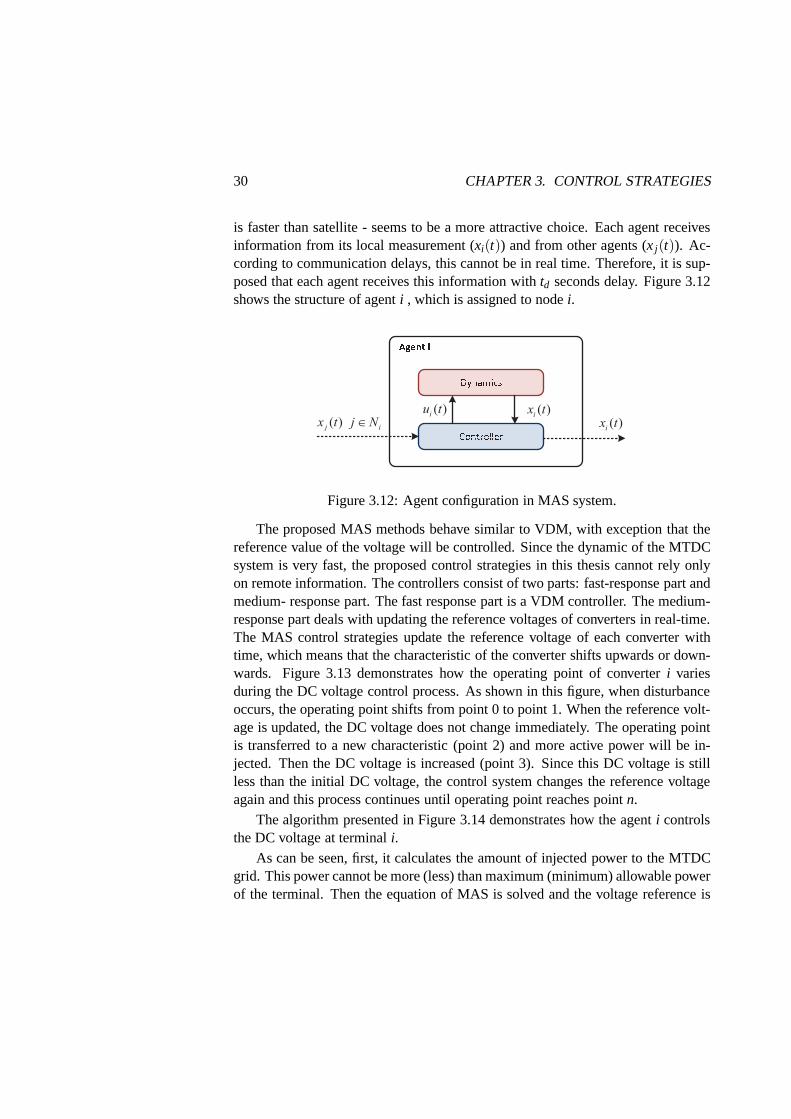
is faster than satellite - seems to be a more attractive choice. Each agent receivesinformation from its local measurement (xi(t)) and from other agents (x j(t)). Ac-cording to communication delays, this cannot be in real time. Therefore, it is sup-posed that each agent receives this information withtd seconds delay. Figure 3.12shows the structure of agenti , which is assigned to nodei.
( )ix t( )
iu t
( )ix t( )
j ix t j N
Figure 3.12: Agent configuration in MAS system.
The proposed MAS methods behave similar to VDM, with exception that thereference value of the voltage will be controlled. Since thedynamic of the MTDCsystem is very fast, the proposed control strategies in thisthesis cannot rely onlyon remote information. The controllers consist of two parts: fast-response part andmedium- response part. The fast response part is a VDM controller. The medium-response part deals with updating the reference voltages ofconverters in real-time.The MAS control strategies update the reference voltage of each converter withtime, which means that the characteristic of the converter shifts upwards or down-wards. Figure 3.13 demonstrates how the operating point of converter i variesduring the DC voltage control process. As shown in this figure, when disturbanceoccurs, the operating point shifts from point 0 to point 1. When the reference volt-age is updated, the DC voltage does not change immediately. The operating pointis transferred to a new characteristic (point 2) and more active power will be in-jected. Then the DC voltage is increased (point 3). Since this DC voltage is stillless than the initial DC voltage, the control system changesthe reference voltageagain and this process continues until operating point reaches pointn.
The algorithm presented in Figure 3.14 demonstrates how theagenti controlsthe DC voltage at terminali.
As can be seen, first, it calculates the amount of injected power to the MTDCgrid. This power cannot be more (less) than maximum (minimum) allowable powerof the terminal. Then the equation of MAS is solved and the voltage reference is

3.4. MULTI-AGENT CONTROL 31
1 2
3n0
,dc iV
,inj iP,inj iP∆
Figure 3.13: TheVdc control process.
Set initial
value
MAS
equation
Local data
measurment
(Recieve remote
data)
max max, , ,inv i inj i rec iP P P£ £
No
YesYes
max, ,
max, ,
inj i inv i
inj i rec i
P
P
P
or
P
=
=
Equations (2.1)
and (2.2)
Figure 3.14: TheVdc control algorithm in each agent.
updated. If the system has reached the desired value, it stops updating referencevalues, otherwise the reference values will be updated again.
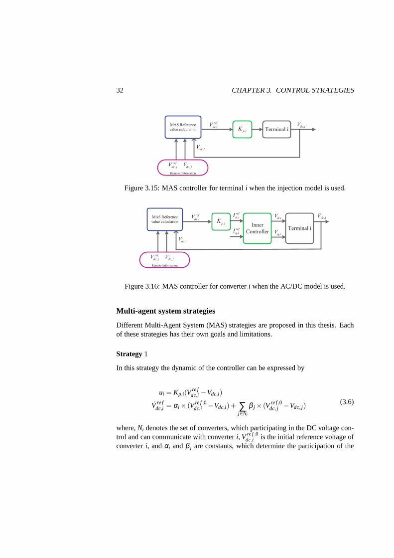
Figures 3.15 and 3.16 show the block diagram of the MAS controller for injec-tion model and AC/DC model, respectively.
32 CHAPTER 3. CONTROL STRATEGIES
,p iK,
ref
dc iVMAS Reference
value calculation,dc iV
,dc iV
Remote Information
,
ref
dc jV ,dc jV
Terminal i
Figure 3.15: MAS controller for terminali when the injection model is used.
,p iK,
ref
dc iVMAS Reference
value calculation,dc iV
,dc iV
Remote Information
,
ref
dc jV ,dc jV
Terminal iInner
Controller
,
ref
d iI
,
ref
q iI
,d iV
,q iV
Figure 3.16: MAS controller for converteri when the AC/DC model is used.
Multi-agent system strategies
Different Multi-Agent System (MAS) strategies are proposed in this thesis. Eachof these strategies has their own goals and limitations.
Strategy 1
In this strategy the dynamic of the controller can be expressed by
ui = Kp,i(Vre fdc,i −Vdc,i)
V re fdc,i = αi × (Vre f,0
dc,i −Vdc,i)+ ∑j∈Ni
β j × (Vre f,0dc, j −Vdc, j)
(3.6)
where,Ni denotes the set of converters, which participating in the DCvoltage con-trol and can communicate with converteri, V re f,0
dc,i is the initial reference voltage ofconverteri, andαi andβ j are constants, which determine the participation of the

3.4. MULTI-AGENT CONTROL 33
local information of agenti and the information from the other agents in the be-havior of agenti, respectively. If there is no communication between agents, thenβ = 0 and only the local information of each agent affects its behavior.
According to the multi-agent theory, if a disturbance happens, this controllertries to make the DC voltages of terminals equal to their initial voltage. But, sincethe power flow in the system has been changed, this is not possible to reach theprevious equilibrium point. Therefore, each controller stops updating the referencevalues when the DC voltage is close enough to the initial value.
Strategy 2
As mentioned in Section 3.3, when a disturbance happens in the MTDC system,the deviation of the DC voltages from their initial voltagesare not exactly equal.Therefore, the power imbalance will not be divided proportional to the droop gains.In [61], we have shown this fact using another argument.
In this strategy, the goal of this controller is to make voltage deviations (xi(t) =Vre f,0
dc,i (t)−Vdc,i(t)) equal.The proposed distributed controller takes the following form:
ui = Kp,i(Vre fdc,i −Vdc,i)
V re fdc,i =−γi ∑
j∈Ni
φi j
((V re f
dc,i −Vdc,i)−(V re fdc, j −Vdc, j)
) (3.7)
whereφi j = φ ji > 0 andγi > 0 are constants. These converters can be consideredas an agent. In this set-up, the state of these converters is the difference betweenits DC voltage setting and the measured DC voltage. These agents with singleintegrator dynamic and DC voltage states can come to a globalagreement on theirstates if they share their states.
Strategy 3
This strategy is a combination of VMM, VDM and MAS strategies. This methodis based on leader-follower MAS theory [62, 63]. In this theory some agents areconsidered as leaders, while other agents are considered asfollowers. Each set offollowers, follows one of the leaders and each agent has its own goal.
The aim of controller is to recover the DC voltage as close as possible tothe initial voltage, while at the same time makes the power distribution propor-tional to the droop gains (Kp,i). To achieve this goal, one agent is selected as the

34 CHAPTER 3. CONTROL STRATEGIES
leader (slack converter), while other agents follow this converter. The consensusis reached for voltage deviation of all buses, therefore theexpected power sharingwill be achieved. On the other hand, reference voltages of all converters follow thereference voltage of the slack converters. Therefore, the voltage will be close tothe initial voltage.
Suppose that converterm, without loss of generality, is regulating DC voltageto its value before the disturbance. The proposed distributed controller takes theform
um = Kp,m(Vre fdc,m−Vdc,m)
Vre fdc,m = KV(V
re f,0dc,m −Vdc,m)−γm ∑
j∈Nm
φm j
((V re f
dc,m−Vdc,m)−(Vre fdc, j −Vdc, j)
) (3.8)
whereKV = 1. For converteri (i 6= m), the control law is like (3.7).The first row of (3.8) (fast response) ensures that the controlled injected cur-
rents are quickly adjusted after a change in the voltage. Thesecond row ensuresthat the voltage is restored at convertermby integral action, and that the controlledinjected currents are proportional to the proportional gains Kp,i at stationarity. Invector-form, (3.8) can be written as
u = KP(Vre fdc −Vdc)
Vre fdc = KV(V
ref,0dc −Vdc)−γγγLLL φ (Vre f −Vdc)
(3.9)
whereγγγ = diag(γi , . . . ,γn), KP is defined as before,KV is an×n matrix whose ele-ments are zero except its m-th diagonal element, which is equal to 1, andLLL φ is theweighted Laplacian matrix of the graph representing the communication topology,whose edge-weights are given byφi j , and which is assumed to be connected.
In [61], we have shown that this controller results in a stable closed loop system(for Injection model) if
λmin
(12
CLLL R+12LLL RC
)+min
iCiKP,i > 0 (3.10)
λmin
(12LLL φ CLLL R+
12LLL RCLLL φ
)≥ 0 (3.11)
whereC = diag([C−11 . . .C−1
n ]) andCi is the aggregated capacitance of con-verter i (see Figure 2.1),LLL R is the weighted Laplacian matrix of the graph rep-resenting the transmission lines whose edges are equal togi j (see (2.3)) andλi is

3.5. SLIDING MODE CONTROL 35
the i-th eigenvalue ofLLL R . We have shown that for a sufficiently largeKP,i anda sufficiently smallγi such that the first condition will be fulfilled. Also, if thetopology of the communication network is identical to the topology of the powertransmission cables up to a positive scaling factor, the second condition will alsobe fulfilled.
3.5 Sliding mode control
As mentioned in chapter 1, Sliding Mode Control (SMC) is a variable structurecontrol, which is originally used for systems whose dynamics can be modelledwith ordinary differential equations [44].
SMC has some features like insensitivity to parameter variations, external dis-turbance rejection and fast dynamic response. Consideringthat the values of theparameters of the system may change and also considering thefast dynamic of theMTDC grid, SMC can be a good option for controlling the MTDC gird. Moreover,if the value of each of the parameters in the system changes (due to uncertainty orany other reason), SMC still has a good performance. On the other hand, since inSMC best approximation of the plant is used, it can control the voltage of a buswithout knowing the exact voltage of adjacent buses. In thisthesis, SMC is appliedto the AC/DC model.
Mathematical background
Two approaches for SMC design are discussed in this thesis: basic control andintegral control:
Basic control
Suppose thatx= x−xre f is the traction error of variablex. Consider a time-varyingsurfaceS(x, t):
S(x, t) = (ddt
+λ )n−1x (3.12)
where,λ is a strictly positive constant andn is the relative degree of the variablex.Sometimes output variableVdc,i is not expressed explicitly based on control inputs.If we differentiate an output variablen times, control inputs appear in the expres-sion. Then, the output variable is told to have relative degree ofn. Remaining on

36 CHAPTER 3. CONTROL STRATEGIES
the manifoldS= 0 is equal to having zero tracking error. SMC converts the track-ing control problem into a first-order differential equation. In such a system, if theerror is negative, it is simply enough to push hard in positive direction [64].
Generally, if the system trajectory satisfies a generalizedLyapunov stabilityrequirement to the surfaceS= 0, there exists a sliding mode on manifoldS= 0.Based on lyapunov stability requirement, the sliding mode exists if u is chosensuch that
12
ddt
S2 ≤−η |S| (3.13)
whereη is a strictly positive constant. Therefore, the state trajectory reaches thesliding surface in less thans(t = 0)/η (s) and slides along the surface towardxre f
exponentially with a time constant equal to1λ [64].
If the dynamics of the system is known, an equivalent controlterm (ueq) ischosen so that the system remains on the sliding surface (S= 0). If the dynamics isnot exactly known, the best estimation of the dynamics is used and the equivalentterm (ueq) is calculated.
u= ueq (3.14)
On the other handu must satisfy the equation (3.15):
u=
{u+ if S(x) > 0
u− if S(x) < 0(3.15)
whereu+ < ueq andu− > ueq. Therefore a switching functionusw= ksgn(S) mustbe added to theu, wherek is a positive scalar and sgn(.) is the sign function.Therefore:
u= ueq−usw (3.16)
Suppose that we have an equation of the general form
x= F +u (3.17)
Consider (3.12) for the case ofn= 1. Then,
S= F +u− xre f (3.18)

3.5. SLIDING MODE CONTROL 37
In order to fulfill the requirement of stability (S= 0), we must have
ueq=−F + xre f (3.19)
For the equations of the general form
x= F +u, (3.20)
equation (3.12) withn= 2 then gives:
S= F +u− xre f +λ ˙x (3.21)
Therefore the equivalent control input must be
ueq=−F −λ ˙x+ xre f (3.22)
Integral control
Based on (3.12), if we consider∫ t
0 x(t ′)dt′ as the error we want to be eliminated,then the sliding surface can be expressed as
S(x, t) =(ddt
+λ )n−1(∫ t
0x(t ′)dt′
)=
= ˙x+2λ x+λ 2∫ t
0x(t ′)dt′
(3.23)
Next, we choose the equivalent control so thatS= 0:if n= 1:
S= F +u− xre f +λ x (3.24)
ueq=−F + xre f −λ x (3.25)
if n= 2
S= F +u− xre f +2λ ˙x+λ 2x (3.26)
ueq=−F −2λ ˙x−λ 2x+ xre f (3.27)

38 CHAPTER 3. CONTROL STRATEGIES
3.6 Application to MTDC system
In this section the SMC controllers are applied AC/DC model of MTDC presentedin 2.1. The output variable can be DC voltage (or active power) and reactive power(or AC voltage). Considering (2.24) and (2.25), if the aim isto control the activepower, we choose the output vectorh1,i . If the DC voltage is of interest,h2,i ischosen as output vector.
h1,i =
[Vdc,i
Iq,i
], h2,i =
[Id,iIq,i .
](3.28)
In this study,Vdc,i has relative degree of 2, because the control inputs appear inVdc,i . However,Id,i andIq,i have relative degree of 1.
If h1,i is considered as output vector, the new output variables canbe written as
[h1,i(1,1)h1,i(2,1)
]=
[Vdc,i
Iq,i
]= Fi(xi)+Bi(xi)ui (3.29)
where,
Fi(xi) =
[F1,i
F2,i
](3.30)
Bi(xi) =
(Ud,i−2r i Id,i)ciVdc,i
(−1li)
(Uq,i−2r i Iq,i)ciVdc,i
(−1li)
(−1li) 0
(3.31)
with
F1,i =(Ud,i −2r iId,i)
ciVdc,if1,i +
(Uq,i −2r i Iq,i)
ciVdc,if2,i+
(
−1
ciV2dc,i
(Ud,i Id,i +Uq,iIq,i − r i(I2d,i + I2
q,i))−Ni
∑i= j
gi j
ci
f3,i
F2 = f2,i
(3.32)
f1,i , f2,i and f3,i in the above equations are given in (2.19).

3.6. APPLICATION TO MTDC SYSTEM 39
Consider now the second output vectorh2,i . The dynamics of terminali, basedon new variables, can be written as
[h2,i(1,1)h2,i(2,1)
]=
[Id,iIq,i
]= Ei(xi)+Diui (3.33)
where
Ei(xi) =
[f2,if1,i
], see (2.19) (3.34)
Di =
[−1li
00 −1
li
](3.35)
The controller structure is shown in Figure 3.17. As long asVdc,i is not equal toits reference voltage, converteri will remain in CPM. In this case the output vectoris h2,i . After Vdc,i reachesVre f
dc,i , the converteri switches to the VCM. In this case
SMC regulatesVdc,i atVre fdc,i and the output vector ish1,i .
_
SMC
Controller
,
ref
inj iP
,inj iP
,
ref
dc iV_
,dc iV
,
ref
d iI
_
,
ref
inj iQ
,inj iQ
ac,
ref
iV _
,ac iV
,
ref
q iI
,d iI
,q iI
,d iV
,q iV
_
_
PI
PI
PI
Terminal i
,
,
,
d i
q i
dc i
I
I
V
æ öç ÷
= ç ÷ç ÷è ø
x
,d iI ,,
,dc iV ,,dc
,q iI ,
_
Figure 3.17: SMC controller for converteri when the AC/DC model is used.
In the figure,Vdc,i , Id,i andIq,i represent the tracking errors ofVdc,i , Id,i andIq,i ,respectively, which are expressed by
Vdc,i =Vdc,i −Vre fdc,i
Id,i = Id,i − I re fd,i
Iq,i = Iq,i − I re fq,i
(3.36)
40 CHAPTER 3. CONTROL STRATEGIES
Suppose that converteri controls the DC voltage and reactive power. Theequivalent control terms for basic and integral controls are chosen as follows:
Basic control
As mentioned in Section 4.2,Vdc,i has relative degree 2, whileId,i and Iq,i haverelative degree 1. For slack terminal, according to (3.19) and (3.22), the equivalentcontrol can be written as
uh1eq,i =−Fi +
[V re f
dc,i −λi˙Vdc,i
I re fq,i
](3.37)
For other terminals, where the output vector ishi2, we obtain the following controlinput :
uh2eq,i =−Ei +
[I re fd,i
I re fq,i
](3.38)
Assuming there is no communication available between terminals and each termi-nal does not have access to DC voltages of other terminals, thenFi(xi) andEi(xi)are not exactly known, but it has a bounded imprecision. As a result we use the bestestimation of these vector fields (indicated byFi(xi) andEi(xi)) to calculate equiv-alent term. In addition, we write the equivalent control terms given in (3.38) and(3.37) asueq,i . Therefore, the controller needs a switching (discontinuous) term asmentioned in (3.16) and (3.15). Forh1,i , this term can be written as
uh1sw,i =
[−k1,isgn(S1,i)−k3,isgn(S3,i)
](3.39)
and forh2,i
uh2sw,i =
[−k2,isgn(S2,i)−k3,isgn(S3,i)
](3.40)
where
S1,i = ˙Vdc,i +λiVdc,i (3.41)
S2,i = Id,i (3.42)
S3,i = Iq,i (3.43)

3.6. APPLICATION TO MTDC SYSTEM 41
andk1,i , k2,i andk3,i are positive constants.In order to have a more smooth control law, the tanh function can be used
instead of sign function. Therefore, the equations can be restated as
uh1sw,i =
[−k1,i tanh(S1,i)−k3,i tanh(S3,i)
](3.44)
uh2sw,i =
[−k2,isgn(S2,i)−k3,isgn(S3,i)
](3.45)
Finally, according to (3.29), (3.33) and (3.16), the complete control input is
uh1i = B−1
i
(uh1
eq,i −uh1sw,i
)(3.46)
Similarly, for h2,i we obtain
uh2i = D−1
i
(ueq,i −uh2
sw,i
)(3.47)
Integral control
If h1,i is chosen as the output vector, the equivalent control inputis
uh1eq,i =−Fi +
[Vre f
dc,i −2λi˙Vdc,i −λ 2
i Vdc,i
I re fq,i −ζi Iq,i
](3.48)
Similarly, for h2,i we have the following control input:
uh2eq,i =−Ei +
[I re fd,i −ξi Id,i
I re fq,i −ζi Iq,i
](3.49)
Switching terms are calculated using (3.39) and (3.40), butthe sliding surfaces aredefined as follows:
S1,i = ˙Vdc,i +2λiVdc,i +λ 2i
∫ t
0Vdc,idt (3.50)
S2,i = Id,i +ξi
∫ t
0Id,idt (3.51)
S3,i = Iq,i +ζi
∫ t
0Iq,idt (3.52)
whereξi andζi are positive constants.

42 CHAPTER 3. CONTROL STRATEGIES
3.7 H∞ control design
In theH∞ control design method, a feedback controller is sought to stabilize theclosed-loop system and satisfy a prescribed level of performance to achieve refer-ence tracking and disturbance attenuation. In this thesis,since all the states of thesystem are measurable, theH∞ state-feedback is chosen as the control strategy.
Let us consider the following state-space representation for an LTI system
x(t) = Ax(t)+B1d(t)+B2u(t)
y(t) = x(t)
z(t) = C1x(t)+D11d(t)+D12u(t) (3.53)
wherex(t)∈Rn is the state vector,y(t)∈R
ny is the measurement vector,z(t)∈Rnz
is the vector of controlled outputs (representing a predefined performance like erroror control effort),d(t) ∈ R
nd is exogenous disturbance vector and process noisesignals with finite energy, andu(t) ∈ R
nu is the control input vector.The first step is to select a pair of inputs and outputs to reflect the system
performance requirements and then design a controller by minimizing the maxi-mum energy-to-energy gain of the corresponding transfer matrix. The H∞ state-feedback controller seeks for
u(t) = Kx (t) (3.54)
to minimize the energy-to-energy gain of the system from disturbanced(t) to out-putz(t). Alternatively, theγ-suboptimalH∞ control problem seeks for a controllerthat yields the energy-to-energy gain less than a positive scalarγ [65]. Note thatthe γ-suboptimal design guarantees that the output vector energy will be boundedby γ‖d‖L2 for all possible bounded energy disturbance inputsd(t). For the sakeof simplicity, we first consider the problem of regulation, i.e., designing the state-feedback controller (3.54) such that the states of the system asymptotically con-verge to zero, regardless of the initial values of the statesor the presence of dis-turbances while the control effort is of affordable magnitude. Indeed, the controldesign objective is not only to regulate the states and reject the exogenous outputdisturbances, but also to keep the control action below a threshold due to the max-imum power limitation of converters. Afterwards, by a mapping, we can easilyhandle the problem of reference tracking in which the statesof the system track adesired values not necessarily zero. We can also use weighting functions to weightminimization of the elements of the vectorz.
Figure 3.18 shows the augmentation of the weighting function with the open-loop system (G(s)) and the state-feedback controller [66].

3.7. H∞ CONTROL DESIGN 43
y x=yW
u
y
zz
z
é ù= ê úë û
uW
(s)G
K
d
u
Figure 3.18: State-feedback controller in the Linear Fractional Transformation(LFT) configuration.
State-feedbackH∞ control design formulation
In this section, we provide theH∞ state-feedback control design formulation interms of a Linear Matrix Inequality (LMI) problem.
Theorem 1: Assuming that the augmented system in Figure 3.18 is describedby the state-space representation (3.53), there exists a state-feedback control law(3.54), which stabilizes the system and guarantees an upperboundγ on the energy-to-energy gain of the closed-loop system from disturbanced(t) to the vectorz(t),if there exist a positive-definiteX ∈ R
n×n andW ∈Rnu×n such that
X +AX +XAT +B2W+WTBT2 B1 XCT
1 +WTDT12
BT1 −γ2I DT
11C1X +D12W D11 −I
< 0 (3.55)
K = WX−1. (3.56)
Proof: See [67].
Note that since it is supposed that the controllers in this method only use thelocal information, we want to design a block diagonal controller so that the com-prising subsystems of (3.53) become decoupled. In this way,each subsystem iscontrolled independently by feeding the state variables ofitself, without needingthe information of other subsystems. In order to derive a block diagonal controllermatrixK , it is required to constrain the structure of LMI variablesX andW in The-orem 1 to be block diagonal. To solve this inequality we use MATLAB LMI tool-box to solve the Theorem 1 which support different structures of the LMI variables

44 CHAPTER 3. CONTROL STRATEGIES
including block diagonal. So far, we have designed a controller for the regulationproblem. Now, we must consider the tracking problem of nonzero reference inputsby performing a mapping on the controller matrixK derived in Theorem 1.
Reference tracking
Consider the open loop system (3.53) without external disturbanced, and letyddenote the desired constant value for outputy. Since in generalyd 6= 0, the statevariablex and control inputu converge to nonzero steady state valuex∗ andu∗,respectively. Therefore, after asymptotic convergence ofthese variables, we have
[A B2
C 0
][x∗
u∗
]=
[0yd
]. (3.57)
By tacking matrix inversion, we can deducex∗ =Myd andu∗ =Nyd. Defining newvariables∆x = x−x∗ and∆u = u−u∗, the tracking problem becomes a regulationproblem for which we solved the controllerK in Theorem 1. Therefore, for thetracking problem we haveu = u∗+∆u = u∗−K∆x = u∗−K(x−x∗). Replacingfor steady state valuesx∗ andu∗, we obtainu = Nyd +K(Myd −x).
The configuration of the closed-loop system for the trackingproblem is shownin Figure 3.19.
Mdy u
( )G sK S
N
+y x=
-
Figure 3.19: Reconfiguration of the closed-loop system for set point tracking.
Application to MTDC system
As stated before, usingH∞ controller, we can reach a specific level of performance.The controller can control the DC voltage and meanwhile can control the injected

3.7. H∞ CONTROL DESIGN 45
power of converters and current of some DC lines. It can also make the partic-ipation of converters proportional to their available headroom. Non of the othermentioned methods, has these capabilities.
In this thesis, we applyH∞ method only on Injection model. According to(2.5), in (3.53) we have:
x(t) = xDC and u(t) = uDC (3.58)
We design anH∞ control for the MTDC system so that for each terminal thetracking error of the DC voltage (deviation of DC voltage from its reference value)is minimized, the control input is of low amplitude and also the currents of one orsome of the DC lines is within a reasonable range. By stackingthese quantities,we construct the vector as shown in Figure 3.18. The weighting functions signifyhow each of these values contribute in the minimization process.
For instance, here, we explain the procedure of selection ofweights for thecontrol inputs. Each converter has a maximum allowable injected power. The dif-ference between this power and the power which is being injected by the converter,is called headroom. We define the headroom index of converteri (Ξi) as
Ξi =ϒi
n∑j=1
ϒi
(3.59)
whereϒi is the available headroom of converteri andn is the number of converters.We determine the gain of each controller proportional to theheadroom index ofeach converter. To achieve this goal we choose gains such that wui = (Ξi)
−1. Nowthe question is which maximum limit of the converter must be consider to calculateϒi . For each converter, we calculate twoϒi , i.e. one when increasingPin j,i, andthe other one when decreasingPin j,i . As a result,H∞ controller uses two differentdroops depending on the disturbance.


Chapter 4
Case studies
4.1 Introduction
Consider the 4-terminal MTDC system shown in Figure 4.1. Theinitial values ofthe voltages at the DC buses, injected powers to the DC buses as well as refer-ence voltages of converters are given in Table 4.1. Also, themaximum allowableinjected powers of converters are shown in this table. The parameters of the DCcables are shown in Table 4.2.
Terminal 4 connects a wind farm to the MTDC system and harvests maximumpower from the wind farm, therefore it does not contribute tothe DC voltage con-trol. This converter also needs to control the AC voltage at wind farms side.
Table 4.1: Initial values of the simulation and reference voltages of terminals forboth SMC and VMM.
Converter 1 Converter 2 Converter 3 Converter 4DCvoltage(p.u.) 1.0 0.9957 1.0009 0.9964
Pin j (p.u.) -0.2824 -0.7143 0.8571 0.1429Vre f
dc,i (pu) 1 1.02 0.98 -Pmax
in j,i 0 2 1 1.5Pmin
in j,i -1 -2 0 0
To compare the results of the control methods, two disturbances have beenconsidered in this chapter. These disturbances are included in two cases. Theperformance of each control method has been studied for one or both cases.
47

48 CHAPTER 4. CASE STUDIES
12R
13R
24R
34R
,1dcV
,2dcV
,3dcV
,4dcV
inj,1P
inj,2P
inj,3P
inj,4P
AC
grid 1
AC
grid 3
AC
grid 2
Wind
Farm
1C
2C
3C
4C
VSC
VSC
VSC
VSC
Figure 4.1: An MTDC system with four terminals.
Table 4.2: Parameters of the DC cables.
L12 L13 L24 L34
Length (km) 500.0 50.0 50.0 500.0Resistance (p.u.) 0.0154 0.0015 0.0015 0.0154
Case1 (Change in wind turbine injected power) As can be seen in Table4.1, initially, the wind farm (converter 4) injects 0.1429(pu) to the MTDC system.At t = 1(s) wind increases and since the converter 4 harvests the maximum powerfrom the wind, its injected active power is increased, with astep, to 0.5(pu).
Case2 (Disconnection of converter)
We study the disconnection of the slack converter in this case. Suppose thatat t = 1(s) terminal 1 is disconnected. Initially, this converter was operating asinverter; therefore, its disconnection leads to active power surplus in the MTDCsystem and as a result, the DC voltage increases.

4.2. STUDY1 49
4.2 Study1
In this study, Case 1 is applied to all control methods. For VMM, it is supposedthat converter 1 is the slack terminal and controlsVdc,1. The converters 2 and 3are working in CPM, therefore they are controllingPin j,2 andPin j,3. As mentionedin section 3.3, in VDM more than one terminal participate in controlling the DCvoltage. The voltage droop constants are given in Table 4.3.As can be seen,converter 4 does not participate in the DC voltage control.
Table 4.3: Voltage droop constants of converters.
Converter 1 Converter 2 Converter 3 Converter 4Kp,i 9 5 1 –
Table 4.4 shows which control methods are applied for each model in this the-sis.
Table 4.4: Table of the methods used in papers
VDM VMM MAS SMC H∞Injection Model X X X X
AC/DC model X X X X
Figure 4.2 shows the variation of theVdc,2 from its initial value in responseto the disturbance mentioned in Case 1. In order to compare the results moreconveniently, in this study we have chosen only one DC voltage. Other DC voltagesshow similar behaviors.
As stated above, the injected active power of converter 4 is increased whichleads to an active power surplus in the MTDC system, which increases the voltagesat the DC buses. In VMM, converter 1, which is the slack converter, must controlthe DC voltage. To this aim, it extract more active power fromthe MTDC system.Then, the DC voltage at bus 1 return to its initial value, but since the MTDC systemoperates at a new operating point, the voltages at other DC buses will not be thesame as their voltages before disturbance.
In VDM, converters 1-3 try to control the DC voltage. As can beseen, appli-cation of this method leads to a steady state voltage deviation.
In this study only one of the MAS strategies is selected. The comparison be-tween MAS strategies is presented in Study 3. In MAS startegy3, both powersharing and returning to a level close to initial voltage areimportant. It is notshown in this figure, but the voltage reaches to steady state at aroundt = 12(s) (see

50 CHAPTER 4. CASE STUDIES
1 1.2 1.4 1.6 1.8 2−0.01
0
0.01
0.02
0.03
0.04
0.05
0.06
Time (s)
∆ V
dc,2
VMM
MAS 3
VDM
H∞
Figure 4.2: Study1: Variation of the voltage at DC bus 2 (∆Vdc,2) when Injectionmodel is used and different control methods are applied. VMM(in red), VDM (inblack), MAS strategy 3 (in blue),H∞ (in green).
figure 4.5). Note that in MAS strategies the communication graph is considered tobe the same as the topology graph of the MTDC system. According to MAS the-ory, if an agent is fixed and does not update its position, all other agents convergeto its position and therefore the solution will not be optimal solution. Consideringthis fact, since the converter 4 does not participate in voltage control, its data is notused as a remote data by other converters. The droop coefficients are the same asVDM.
It can be seen that application ofH∞ leads to a voltage deviation very smallerthan the VDM. This is reasonable because theH∞ uses a static feedback here andtherefore its response should be like VDM, which uses a proportional controller.On the other hand, sinceH∞ uses an optimization and minimizes the voltage de-viation, the steady state voltage deviation must be smallerthan VDM. It must benoted that for applying theH∞ method in this thesis, the limitations of the ACgrids are not considered.
Figure 4.3 shows the variation of voltages at the DC buses when AC/DC modelis used. As shows in the figure, the behavior of the system is very much like thecase where Injection model is used, however, since in AC/DC model the dynamicof the AC part is also considered, the injected active power cannot change as fastas in the previous case and therefore, the voltage variations are larger.

4.2. STUDY1 51
1 1.2 1.4 1.6 1.8 2−0.01
0
0.01
0.02
0.03
0.04
0.05
0.06
Time (s)
∆ V
dc,2
MAS 3
VDM
VMM
Basic SMC
Integral SMC
Figure 4.3: Study1: Variation of the voltage at DC bus 2 (∆Vdc,2) when AC/DCmodel is used and different control methods are applied. VMM(in red), VDM (inblack), MAS strategy 3 (in blue), basic SMC (in green), integral SMC (in dashedgreen).
Moreover, in this model, the two SMC control methods are alsoimplemented.As can be seen, application of both SMC methods leads to a behavior like whenVMM is applied, but with smaller overshoot and faster response. The voltagewhen integral SMC is applied has less overshoot comparing towhen basic SMCis applied, but it has a small oscillation. SinceVdc,2 is shown in this figure andconsidering that the operating point has been changed, the final values ofVdc,2 isdifferent from its initial values. However, the final valuesof Vdc,1 is the same as itsinitial values if VMM and SMC methods are applied and if the slack converter cansuccessfully control the DC voltage.
To study how the converters share the active power change, itis desired tocompare the final values of the injected powers of different terminals. Table 4.5shows changes in the injected active powers of converters when different controlstrategies are used. Since in the next section, SMC and VMM will be studied, inorder to cover the power distribution from all control methods, the injection modelis used to achieve the results of this table in this section. However, to cover theresults of SMC, in the next study, the results from the AC/DC model is used forcompleting the table. Only one of the MAS methods has been chosen for thiscomparison.
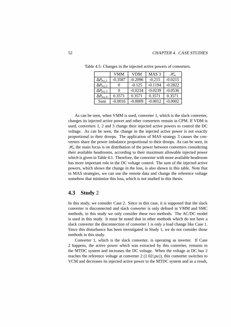
52 CHAPTER 4. CASE STUDIES
Table 4.5: Changes in the injected active powers of converters.
VMM VDM MAS 3 H∞∆Pin j,1 -0.3587 -0.2096 -0.215 -0.0215∆Pin j,2 0 -0.125 -0.1194 -0.2822∆Pin j,3 0 -0.0234 -0.0239 -0.0536∆Pin j,4 0.3571 0.3571 0.3571 0.3571Sum -0.0016 -0.0009 -0.0012 -0.0002
As can be seen, when VMM is used, converter 1, which is the slack converter,changes its injected active power and other converters remain in CPM. If VDM isused, converters 1, 2 and 3 change their injected active powers to control the DCvoltage. As can be seen, the change in the injected active power is not exactlyproportional to their droops. The application of MAS strategy 3 causes the con-verters share the power imbalance proportional to their droops. As can be seen, inH∞ the main focus is on distribution of the power between converters consideringtheir available headrooms, according to their maximum allowable injected powerwhich is given in Table 4.1. Therefore, the converter with more available headroomhas more important role in the DC voltage control. The sum of the injected activepowers, which shows the change in the loss, is also shown in this table. Note thatin MAS strategies, we can use the remote data and change the reference voltagesomehow that minimize this loss, which is not studied in thisthesis.
4.3 Study2
In this study, we consider Case 2. Since in this case, it is supposed that the slackconverter is disconnected and slack converter is only defined in VMM and SMCmethods, in this study we only consider these two methods. The AC/DC modelis used in this study. It must be noted that in other methods which do not have aslack converter the disconnection of converter 1 is only a load change like Case 1.Since this disturbance has been investigated in Study 1, we do not consider thosemethods in this study.
Converter 1, which is the slack converter, is operating as inverter. If Case2 happens, the active power which was extracted by this converter, remains inthe MTDC system and increases the DC voltage. When the voltage at DC bus 2reaches the reference voltage at converter 2 (1.02(pu)), this converter switches toVCM and decreases its injected active power to the MTDC system and as a result,
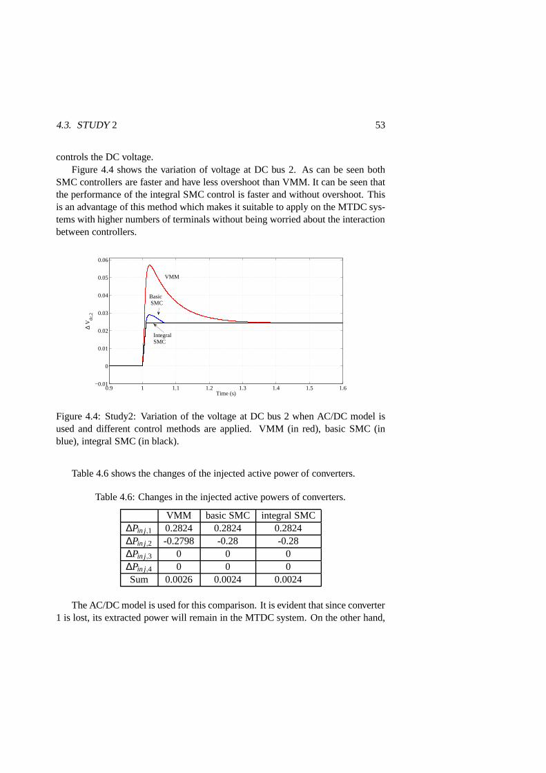
4.3. STUDY2 53
controls the DC voltage.Figure 4.4 shows the variation of voltage at DC bus 2. As can beseen both
SMC controllers are faster and have less overshoot than VMM.It can be seen thatthe performance of the integral SMC control is faster and without overshoot. Thisis an advantage of this method which makes it suitable to apply on the MTDC sys-tems with higher numbers of terminals without being worriedabout the interactionbetween controllers.
0.9 1 1.1 1.2 1.3 1.4 1.5 1.6−0.01
0
0.01
0.02
0.03
0.04
0.05
0.06
Time (s)
∆ V
dc,2
IntegralSMC
Basic SMC
VMM
Figure 4.4: Study2: Variation of the voltage at DC bus 2 when AC/DC model isused and different control methods are applied. VMM (in red), basic SMC (inblue), integral SMC (in black).
Table 4.6 shows the changes of the injected active power of converters.
Table 4.6: Changes in the injected active powers of converters.
VMM basic SMC integral SMC∆Pin j,1 0.2824 0.2824 0.2824∆Pin j,2 -0.2798 -0.28 -0.28∆Pin j,3 0 0 0∆Pin j,4 0 0 0Sum 0.0026 0.0024 0.0024
The AC/DC model is used for this comparison. It is evident that since converter1 is lost, its extracted power will remain in the MTDC system.On the other hand,

54 CHAPTER 4. CASE STUDIES
since converter 2 is the next slack converter, it should extract this power surplusfrom the MTDC system. However, since the operating point hasbeen changed andas a result the loss in the MTDC system has been changed, thesetwo quantities arenot equal.
4.4 Study3
In this study, we focus on MAS control strategies and consider Case 1. OnlyAC/DC model, which is more accurate, is chosen for this study.
Figure 4.5 shows the variation of the DC voltage at bus 2.
2 4 6 8 10 12 14 16−0.01
0
0.01
0.02
0.03
0.04
0.05
0.06
Time (s)
∆ V
dc,2
MAS 2
MAS 3
MAS 1
Figure 4.5: Study3: Variation of the voltages at DC bus 2 for different MAS strate-gies when the AC/DC model is used. MAS strategy 1 (in green), MAS strategy 2(in black), MAS strategy 3 (in blue).
In MAS strategy 1, the voltage is going to return to a level close to its initialvalue. In MAS strategy 2, the behavior of the voltage is not supposed to be so muchdifferent with VDM. The focus in this strategy is on the powersharing betweenconverters proportional to their droops. As mentioned in study 1, in MAS strategy3 the voltage return to a level closed to its initial value andthe power sharing willbe proportional to the droops.

4.4. STUDY3 55
Since MAS controllers use remote information, the communication delay mayaffect the response of these strategies. Therefore, in thisstudy the effect of delayis also considered. There are different values given for delay in the literature [68].The sources of delay are measurement delay and communication delay. The formerdepends on the technology of measurement devices, while thelatter depends on thetechnology being used for transferring data. If fiber optic technology is used, thedelay can be considered around 100(ms), while the satellite technology has a delayaround 700(ms).
If a constant delay equal totd = 100(ms) is considered, the variation of thevoltage at DC bus 2 is shown in Figure 4.6.
1 1.2 1.4 1.6 1.8 2 2.2 2.4 2.6 2.8 3−1
−0.5
0
0.5
Time (s)
∆ V
dc,2
MAS 2 MAS 3
MAS 1
Figure 4.6: Study3: Variation of the voltage at DC bus 2 when there is a delay oftd = 100(ms). The AC/DC model is used and different MAS strategies are applied.
As can be seen, MAS strategy 1 is the most sensitive strategy to the delayand becomes unstable. The delay cause MAS strategy 2 to have larger voltagedeviation, but MAS strategy 3 controls the DC voltage and returns to a level itsinitial value. Of course, by changing the values of the MAS controllers, theirsensitivity to delay will change. Longer delays make the convergence of the MASstrategy slow and can even lead to instability (see [61]). Inorder to increase theconvergence speed, we can increaseγi . Note that, in this study we suppose thatγ1 =γ2 = γ3 = γ . However, in the presence of delay, the largerγ can even worsen theresults. The effect of the parameters on the behavior of the system in the presenceof delay has not been investigated analytically in this thesis.

56 CHAPTER 4. CASE STUDIES
Next, we study the difference between voltage at each converter and its ref-erence voltage,∆ure f
i = Vre fdc,i −Vdc,i . To show the behavior of∆ure f
i , only MASstrategy 3 has been selected.
Figure 4.7 shows the change in∆ure fi for participating converters in MAS
strategy 3. As shown in the figure, they converge to a common value at aroundt = 12(s). Since the∆ure f
i for all converters will be the same, the changes of theirinjected active powers only depend on their droops. It must be noted that the con-vergence of the MAS strategy 2 is much faster than MAS strategy 3.
1 2.5 4.5 6.5 8.5 10.5 12.5 14.5−0.052
−0.049
−0.046
Time (s)
∆ u ire
f
u3ref
u1ref
u2ref
Figure 4.7: Study 3: Variation of the voltage at DC buses fromtheir referencevalues with MAS 3 control strategy. converter 1 (in red), converter 2 (in black),converter 3 (in blue).
Next, we study the contribution ofα andβ in MAS strategy 1.As mentioned in Chapter 3,α is the weight we give to the local information,
while β is the weight of remote information. Considering that the wide-area com-munication can not be without delay, if we considerβ to be large, it can causestability problems. Figure 4.8 shows the response of the system for td = 50(ms)andβ = 1 andβ = 1.5. The variation of the voltage at DC bus 2 is stable forβ = 1and the oscillations will be damped after 3(s) but for β = 1.5 it is unstable.
4.5 Comments
The VDM method used in this thesis, uses local information, i.e. each converteruses its own DC voltage. No Proportional Integral (PI) or Integral (I) controller isused to implement this controller and it is supposed that if adisturbance happens,

4.5. COMMENTS 57
0.9 1 1.1 1.2 1.3 1.4 1.5 1.60
0.05
0.4
Time (s)
∆ V
dc,2
β=1, td=50 (ms)
β=1.5, td=50 (ms)
Figure 4.8: Study 3: Variation of the voltage at DC bus 2 with MAS 1 control andtd = 50(ms) andβ = 1 (in blue) andβ = 1.5 (in black).
converters inject exactly the active power according to their droop curves and thereis no mismatch.
1
1 GT s+dcVD ,inj iPD
dcVD
,inj iP
*
,inj iP
iK
PI,inj iP-
iK-1
sdcVD ,inj iPD
ia
1
iK
-
-
(a) ( )b
(c)
Figure 4.9: Two other proposed schematics for implementingVDM: (a) schemeI ,(b) schemeI (reduced), (c) schemeII
Figure 4.9 shows two other schemes for VDM. In the first scheme(scheme

58 CHAPTER 4. CASE STUDIES
I ), which is shown in Figure 4.9 (a), in addition to the proportional gain (Ki) an Icontroller (with coefficientαi) is also utilized. This scheme is reduced as shownin Figure 4.9 (b), whereTG = 1
Ki αi[69]. In the second scheme (schemeII ), a PI
controller is used (Figure 4.9 (c)) andP∗in j,i is the expected injected active power
according to the voltage droop curve. Both PI and I controllers make sure thatthe actual injected power will be equal to the desired injected power (based on thedroop).
Although one can call it a slope voltage controller, since the VDM controllersin this thesis use local information and considering that the DC voltage is not aglobal variable like frequency in AC system, the proposed system in this thesishas the same steady state results as two other methods. To show this, Study 1 issimulated again and the results are compared together. Figure 4.10 shows behav-ior of Vdc,1 with changes in the injected active power (Pin j,1) for all VDM controlschemes. The system is operating at the point(Pin j,1,Vdc,1), which is marked witha circle. After disturbance, the voltage in all methods reach to the same final value,which is marked with a cross. The only difference between these methods is theirdynamic behavior. The other terminals show similar behaviors. As can be seen,the final value which both controllers reach to, are the same.
−0.4921 −0.2824
1
1.0233
Injected active power (pu)
DC
vol
tage
(pu
)
O
X
Figure 4.10: The voltage against the injected active power at DC bus 1: VDMpresented in this thesis (in black), VDM schemeI (in blue), VDM schemeII (ingreen) and the steady-state characteristic (in dashed red).
Chapter 5
Conclusion and future work
5.1 Conclusion
This thesis has covered the issues regarding the control of the DC voltage in Multi-Terminal high-voltage Direct-Current (MTDC) systems. After a literature review,the MTDC system has been modeled. Two modeling approaches have been pre-sented for the purpose of this thesis: Injection model and AC/DC model. In the In-jection model, only the DC grid has been considered, while inthe AC/DC model,the dynamic of the converter, the AC filter and the phase reactor connecting theterminal to the AC grid has also been considered. The AC systems have been mod-eled with their Thevenin equivalents and it has been supposed that the Theveninvoltage has constant magnitude and phase. The modeling has been done in MAT-LAB/Simulink and a 4-terminal MTDC system has been chosen for the case stud-ies. This grid is connected to three AC grids and one wind farm. Comparing theresults in Figures 4.2 and 4.3, it is evident that the only difference of these modelsis in their transient response, where the AC/DC model shows larger variations, buttheir steady-state response is the same. Depending on the scope of the study, wecan choose one of these models. If including detailed model of AC grid is of in-terest, the AC/DC model has this capability to add it. On the other, if only the DCgrid behavior is of interest, the Injection model can be used.
Two main methods Voltage Droop Method (VDM) and Voltage Margin Method(VMM), which are presented in the literature, have been discussed. Then, two se-ries of control methods presented. The first series of control methods are Multi-Agent System (MAS) control methods. These control methods can be consideredas modified VDM. In this method the reference voltage of each controller is up-
59

60 CHAPTER 5. CONCLUSION AND FUTURE WORK
dated continuously after disturbance happens. These methods use both remote andlocal information, but do not rely only on remote information. When remote in-formation is not available, these methods simply operate like VDM. Each of thesecontrol methods has their own aim in control.
When MAS strategy 1 has been applied to the MTDC system, the DCvoltagehas returned to a level close to their initial values. Then wehave developed theMAS controller further and presented MAS strategies 2 and 3.Application ofMAS strategies 2 and 3 has resulted in equal deviation of DC voltages from theirreference values. As a result, the power has been distributed equal to the droopconstants (similar to the frequency control in AC grids).
We have shown how the power mismatch after a distribution is distributed be-tween different converters. We have also shown the changes in the loss of theMTDC system due to application of different control strategies in Tables 4.5 and4.6. In MAS strategies we can optimize the amount of this lossusing remote infor-mation, but it has not been addressed in this thesis.
Since MAS strategies use remote information and remote information maycomes with delay, a sample delay of 100(ms) has been chosen and the MAS strate-gies have been implemented for this delay. We have shown in figure 4.6 that theMAS strategy 3 has the best performance in the presence of delay.
We have simulated all above control methods using both Injection and AC/DCmodels. The results have shown the effectiveness of the control methods. It hasbeen shown in figures 4.2 and 4.3 that the behavior of the system for these twomodels are similar but the voltage deviation is different.
The second group of control methods have been presented in this thesis in-cludes two Sliding Mode Control (SMC) methods andH∞. This group use onlylocal information. We have implemented the SMC controllers, basic and integral,on AC/DC model andH∞ on Injection model.
We have developed the aforementioned SMC control method using a philoso-phy similar to VMM, i.e., at each time only one of the converters controls the DCvoltage (as slack converter) and other converters control their injected active pow-ers. Because of this similarity, these methods have been compared together. Thesimulation results have shown that both SMC controllers cancontrol the DC volt-age in MTDC system very fast and with less overshoot comparedto VMM. Thenwe have compared the performances of the two SMC control methods with eachother and have shown that in the case of changing the slack converter, basic SMCcontrols the voltage with small overshoot while integral SMC controls the voltagealmost without overshoot. Consequently we have concluded that it is possible tochoose an even smaller voltage margin, which, unlike VMM, makes this method

5.2. FUTURE WORK 61
suitable for MTDC systems with high number of terminals.Finally, we have appliedH∞ control on the MTDC system. We have shown that
it results in a very small voltage deviation after disturbance. This control methodmakes its possible to not only control the voltage, but also limit the injected activepowers and weight the contribution of different convertersproportional to theiravailable headroom.
5.2 Future work
As seen in the simulation results, the delay has an negative effect on the perfor-mance of MAS control methods. It would be interesting to study the effect of delayon the stability of different MAS methods. Considering thatthe performance of thecontroller for a given delay was different in Injection model and AC/DC model, itis important to analyse these effect separately for each model. Moreover, study ofeffect of time varying delays on the proposed MAS controllers can be interesting.
The models presented in this thesis can be further developedto be able to iden-tify and analyze relevant electromechanical dynamics suchas rotor angle stability,voltage stability and frequency stability.
Also supplementary controls (such as Power Oscillation Damping (POD)) canbe developed for the converters to improve dynamical performance of the AC/DCsystem. The impact of the proposed DC voltage control strategies in this thesis andthe aforementioned supplementary controls on the hybrid AC/DC system can bestudied. The aim is to fulfill N-1 criterion for both MTDC and AC systems.
Different market and operation issues can be considered in this MTDC system.In the hourly operation of the system, balance between production and consump-tion has to be kept continuously in an economical and reliable way, consideringproduction and transmission limits. The continuous balance is kept with FrequencyContainment Reserves (FCR) (frequency controlled power plants that keep enoughmargins for this) which is distributed between power plantsin different regions.Used FCR are restored using Frequency Restoration Reserves(FRR) which in themarket means accepted bids to the regulating market. In manysystems there is alsoan Automatic Generation Control (AGC) system which automatically redistributethe production in order to fulfil requirements concerning security limits and eco-nomic generation. The question is how can FCR between the asynchronous ACsystems connected by MTDC system be coordinated?
An important issue is the set-up of the AGC systems and the needed control.The instant reaction after a contingency in, e.g., the MTDC system causes direct

62 CHAPTER 5. CONCLUSION AND FUTURE WORK
changes in the AC systems. This may not be efficient from internal bottleneck pointof view and/or from economic point of view. This then means a)the instant reactionhas to be distributed in such a way that AC system stability ismaintained, b) eachAGC system must be set up in order to consider the price signals so an economicoperation is obtained, c) there must be a coordination between the different ACsystems so one do not get a suboptimum in each system, i.e., re-distribute thepower between the different AC systems in an efficient way, d)there must be asystem set-up so the correct price signals can be consideredin the controllers,e.g. through a real time pricing system. Therefore, the distributed coordinationof different operational zones can be studied.

Bibliography
[1] C.Bayliss and B. Hardy.Transmission and Distribution electrical engineer-ing. Elsevier, 2007.
[2] T. Ackerman. Transmission systems for offshore wind farms. IEEE PowerEngineering Review, pages 124–129, 2002.
[3] W. Long and S. Nilsson. Hvdc transmission: yesterday andtoday.Power andEnergy Magazine, IEEE, 5(2):22–31, March 2007.
[4] N. Flourentzou, V. G. Agelidis, and G. D. Demetriades. Vsc-based hvdcpower transmission systems: An overview.IEEE Transactions on PowerElectronics, 24(3):592–602, 2009.
[5] Jiuping Pan, R. Nuqui, K. Srivastava, T. Jonsson, P. Holmberg, and Y.-J.Hafner. Ac grid with embedded vsc-hvdc for secure and efficient power de-livery. In Energy 2030 Conference, 2008. ENERGY 2008. IEEE, pages 1–6,Nov 2008.
[6] Johansson S.G., G. Asplund, E. Jnasson, G., and R. Rudervall. Power systemstability benefits with vsc dc-transmission systems. InCIGRE session, 2004.
[7] Hvdc light: It’s time to connect. Technical Report MSU-CSE-00-2, ABB,December 2012.
[8] E. Prieto-Araujo, F. D. Bianchi, A. Junyent-Ferré, and O. Gomis-Bellmunt.Methodology for droop control dynamic analysis of multiterminal vsc-hvdcgrids for offshore wind farms. IEEE Transactions on Power Delivery,26(4):2476–2485, 2011.
[9] M.P. Bahrman and B.K. Johnson. The abcs of hvdc transmission technolo-gies.Power and Energy Magazine, IEEE, 5(2):32–44, March 2007.
63

64 BIBLIOGRAPHY
[10] S. Cole, J. Beerten, and R. Belmans. Generalized dynamic vsc mtdc modelfor power system stability studies.Power Systems, IEEE Transactions on,25(3):1655 –1662, aug. 2010.
[11] O. Gomis-Bellmunt, J. Liang, J. Ekanayake, and N. Jenkins. Voltage-currentcharacteristics of multiterminal hvdc-vsc for offshore wind farms. ElectricPower Systems Research, 81(2):440–450, 2011.
[12] E. Koldby and M. Hyttinen. Challenges on the road to an offshore hvdc gird.In Nordic wind power conference 2009, Sep 2009.
[13] N.M. Kirby, M.J. Luckett, L. Xu, and W. Siepmann. Hvdc transmission forlarge offshore windfarms. InAC-DC Power Transmission, 2001. Seventh In-ternational Conference on (Conf. Publ. No. 485), pages 162–168, Nov 2001.
[14] Dawei Xiang, L. Ran, J.R. Bumby, P.J. Tavner, and S. Yang. Coordinatedcontrol of an hvdc link and doubly fed induction generators in a large offshorewind farm.Power Delivery, IEEE Transactions on, 21(1):463–471, Jan 2006.
[15] Lie Xu, Liangzhong Yao, and Christian Sasse. Grid integration of large dfig-based wind farms using vsc transmission.Power Systems, IEEE Transactionson, 22(3):976–984, Aug 2007.
[16] Dirk Van Hertem and Mehrdad Ghandhari. Multi-terminalVSC HVDC forthe European supergrid: Obstacles.Renewable and Sustainable Energy Re-views, 14(9):3156–3163, December 2010.
[17] L. Xu and L. Yao. Dc voltage control and power dispatch ofa multi-terminalhvdc system for integrating large offshore wind farms.IET Renewable PowerGeneration, 5(3):223–233, 2011.
[18] R. T. Pinto, S. F. Rodrigues, P. Bauer, and J. Pierik. Comparison of directvoltage control methods of multi-terminal dc (mtdc) networks through mod-ular dynamic models. InProceedings of the 2011 14th European Conferenceon Power Electronics and Applications, EPE 2011, 2011.
[19] L. Xu and L. Yao. Dc voltage control and power dispatch ofa multi-terminalhvdc system for integrating large offshore wind farms.Renewable PowerGeneration, IET, 5(3):223–233, May 2011.

BIBLIOGRAPHY 65
[20] T. Haileselassie and K. Uhlen. Multiterminal hvdc for offshore windfarmscontrol strategy. InEuropean Power Electronics Energy Chapter Seminar2009, pages 1–6, Nov 2009.
[21] T. Nakajima and S. Irokawa. A control system for hvdc transmission byvoltage sourced converters. InPower Engineering Society Summer Meeting,1999. IEEE, volume 2, pages 1113 –1119 vol.2, 1999.
[22] C. Dierckxsens, K. Srivastava, M. Reza, S. Cole, J. Beerten, and R. Belmans.A distributed dc voltage control method for vsc mtdc systems. Electric PowerSystems Research, 82(1):54–58, 2012.
[23] T. Haileselassie, K. Uhlen, and T. Undeland. Control ofmultiterminal hvdctransmission for offshore wind energy. InNordic Wind Power Conference,Sep 2009.
[24] C Ismunandar, AA van der Meer, M Gibescu, RL Hendriks, and WL Kling.Control of multi-terminal vsc-hvdc for wind power integration using thevoltage-maring method. InProc. 9th Int. Workshop on Large-Scale Integra-tion of Wind Power Into Power Systems as Well as on Transmission Networksfor Offshore Power Plants, pages 18–19.
[25] F. D. Bianchi and O. Gomis-Bellmunt. Droop control design for multi-terminal vsc-hvdc grids based on lmi optimization. InProceedings of theIEEE Conference on Decision and Control, pages 4823–4828, 2011.
[26] N.R. Chaudhuri and B. Chaudhuri. Adaptive droop control for effectivepower sharing in multi-terminal dc (mtdc) grids.Power Systems, IEEE Trans-actions on, 28(1):21–29, Feb 2013.
[27] A.S. Abdel-Khalik, A.M. Massoud, A.A. Elserougi, and S. Ahmed. Optimumpower transmission-based droop control design for multi-terminal hvdc ofoffshore wind farms. Power Systems, IEEE Transactions on, 28(3):3401–3409, Aug 2013.
[28] R. Eriksson, J. Beerten, M. Ghandhari, and R. Belmans. Optimizing dc volt-age droop settings for ac/dc system interactions.Power Delivery, IEEE Trans-actions on, 29(1):362–369, Feb 2014.
[29] Temesgen M. Haileselassie and Kjetil Uhlen. Frequencysensitivity analysisof ac grids connected to mtdc grid. InAC and DC Power Transmission, 2010.ACDC. 9th IET International Conference on, pages 1–5, Oct 2010.

66 BIBLIOGRAPHY
[30] Temesgen M. Haileselassie and Kjetil Uhlen. Impact of DC Line VoltageDrops on Power Flow of MTDC Using Droop Control.IEEE Transactionson Power Systems, 27(3):1441–1449, August 2012.
[31] J. Beerten, D. Van Hertem, and R. Belmans. Vsc mtdc systems with a dis-tributed dc voltage control - a power flow approach. In2011 IEEE PESTrondheim PowerTech: The Power of Technology for a Sustainable Society,POWERTECH 2011, 2011.
[32] T.M. Haileselassie and K. Uhlen. Impact of dc line voltage drops on powerflow of mtdc using droop control.Power Systems, IEEE Transactions on,27(3):1441–1449, Aug 2012.
[33] N. R. Chaudhuri, R. Majumder, B. Chaudhuri, and J. Pan. Stability analysisof vsc mtdc grids connected to multimachine ac systems.IEEE Transactionson Power Delivery, 26(4):2774–2784, 2011.
[34] N.R. Chaudhuri, R. Majumder, B. Chaudhuri, Jiuping Pan, and R. Nuqui.Modeling and stability analysis of mtdc grids for offshore wind farms: Acase study on the north sea benchmark system. InPower and Energy SocietyGeneral Meeting, 2011 IEEE, pages 1–7, July 2011.
[35] J.M. Solanki, S. Khushalani, and N.N. Schulz. A multi-agent solution todistribution systems restoration.Power Systems, IEEE Transactions on,22(3):1026–1034, Aug 2007.
[36] S.D.J. McArthur, E.M. Davidson, V.M. Catterson, A.L. Dimeas, N.D.Hatziargyriou, F. Ponci, and T. Funabashi. Multi-agent systems for powerengineering applications;part i: Concepts, approaches, and technical chal-lenges.Power Systems, IEEE Transactions on, 22(4):1743–1752, Nov 2007.
[37] T. L. Vandoorn, B. Meersman, L. Degroote, B. Renders, and L. Vandevelde.A control strategy for islanded microgrids with dc-link voltage control.IEEETransactions on Power Delivery, 26(2):703–713, 2011.
[38] S.D.J. McArthur, E.M. Davidson, V.M. Catterson, A.L. Dimeas, N.D.Hatziargyriou, F. Ponci, and T. Funabashi. Multi-agent systems for powerengineering applications;part ii: Technologies, standards, and tools for build-ing multi-agent systems.Power Systems, IEEE Transactions on, 22(4):1753–1759, Nov 2007.

BIBLIOGRAPHY 67
[39] Fenghui Ren, Minjie Zhang, D. Soetanto, and XiaoDong Su. Conceptualdesign of a multi-agent system for interconnected power systems restoration.Power Systems, IEEE Transactions on, 27(2):732–740, May 2012.
[40] T. Nagata and H. Sasaki. A multi-agent approach to powersystem restoration.Power Systems, IEEE Transactions on, 17(2):457–462, May 2002.
[41] Hengxuan Li, Haishun Sun, Jinyu Wen, Shijie Cheng, and Haibo He. A fullydecentralized multi-agent system for intelligent restoration of power distribu-tion network incorporating distributed generations [application notes].Com-putational Intelligence Magazine, IEEE, 7(4):66–76, Nov 2012.
[42] Hai Feng Wang, H. Li, and H. Chen. Coordinated secondaryvoltage con-trol to eliminate voltage violations in power system contingencies. PowerSystems, IEEE Transactions on, 18(2):588–595, May 2003.
[43] M. Nazari and M. Ghandhari. Application of multi-agentcontrol to multi-terminal hvdc systems. InIEEE Electrical Power and Energy Conference(EPEC) 2013, Aug 2013.
[44] K.D. Young, V.I. Utkin, and U. Ozguner. A control engineer’s guide to slidingmode control.Control Systems Technology, IEEE Transactions on, 7(3):328–342, May 1999.
[45] H.K.Khalil. Nonlinear Systems. Prentice Hall, New Jersey, 2002.
[46] F. Pourboghrat, F. Farid, C.J. Hatziadoniu, Morteza Daneshdoost,F. Mehdian, and M. Lotfalian. Local sliding control for damping interareapower oscillations.Power Systems, IEEE Transactions on, 19(2):1123–1134,May 2004.
[47] A. Moharana and P.K. Dash. Input-output linearizationand robust sliding-mode controller for the vsc-hvdc transmission link.Power Delivery, IEEETransactions on, 25(3):1952–1961, July 2010.
[48] Niranjan Nayak, Sangram Keshari Routray, and Pravat Kumar Rout. Statefeedback robust h-infinity controller for transient stability enhancement ofvsc-hvdc transmission systems.Procedia Technology, 4(0):652 – 660, 2012.2nd International Conference on Computer, Communication,Control and In-formation Technology( C3IT-2012) on February 25 - 26, 2012.

68 BIBLIOGRAPHY
[49] H-infinity controller for enhancement in vsc-hvdc systen with parallel aclines. International journal of power and energy conversion, 1(2/3):215–242,2009.
[50] L. Xu, L. Yao, and M. Bazargan. Dc grid management of a multi-terminalhvdc transmission system for large offshore wind farms. In1st InternationalConference on Sustainable Power Generation and Supply, SUPERGEN ’09,2009.
[51] A. Yazdani and R. Iravani.Voltage sourced converters in power systems:modeling, control and applications. John Wiley, New Jersey, 2010.
[52] C.Ismunandar. Control of multi-terminal vsc-hvdc foroffshore wind powerintegration. Master thesis, Delft University of Technology, Delft, Nether-lands, August 2010.
[53] J. Dai, Y. Phulpin, A. Sarlette, and D. Ernst. Impact of delays on a consensus-based primary frequency control scheme for ac systems connected by a multi-terminal hvdc grid. In2010 IREP Symposium - Bulk Power System Dynamicsand Control - VIII, IREP2010, 2010.
[54] J. Dai, Y. Phulpin, A. Sarlette, and D. Ernst. Coordinated primary frequencycontrol among non-synchronous systems connected by a multi-terminal high-voltage direct current grid. Generation, Transmission Distribution, IET,6(2):99 –108, february 2012.
[55] K. R. Padiyar and N. Prabhu. Modelling, control design and analysis of vscbased hvdc transmission systems. In2004 International Conference on PowerSystem Technology, POWERCON 2004, volume 1, pages 774–779, 2004.
[56] Jun Liang, O. Gomis-Bellmunt, J. Ekanayake, and N. Jenkins. Control ofmulti-terminal vsc-hvdc transmission for offshore wind power. In PowerElectronics and Applications, 2009. EPE ’09. 13th EuropeanConference on,pages 1 –10, sept. 2009.
[57] B. K. Johnson, R. H. Lasseter, F. L. Alvarado, and R. Adapa. Expandablemultiterminal dc systems based on voltage droop.IEEE Transactions onPower Delivery, 8(4):1926–1932, 1993.
[58] P. Karlsson and J. Svensson. Dc bus voltage control for adistributed powersystem.Power Electronics, IEEE Transactions on, 18(6):1405 – 1412, nov.2003.

BIBLIOGRAPHY 69
[59] Dimos V. Dimarogonas and Karl H. Johansson. Stability analysis for multi-agent systems using the incidence matrix: Quantized communication and for-mation control.Automatica, 46(4):695–700, April 2010.
[60] M. Mesbahi and M. Egerstedt.Graph theoric methods in multiagent net-works. princeton university press, New Jersey, 2010.
[61] M. Andreasson, M. Nazari, D. Dimarogonas, H. Sandberg,K.H. Johansson,and M. Ghandhari. Distributed voltage and current control of vsc multi-terminal high-voltage direct current transmission systems. InWrold congressof internation federation of automatic control, Aug 2014.
[62] G. Ferrari-Trecate, M. Egerstedt, A. Buffa, and M. Ji.Hybrid Systems: Com-putation and Control. Springer, Germany, 2006.
[63] D.V. Dimarogonas, T. Gustavi, M. Egerstedt, and Xiaoming Hu. On the num-ber of leaders needed to ensure network connectivity. InDecision and Con-trol, 2008. CDC 2008. 47th IEEE Conference on, pages 1797–1802, Dec2008.
[64] W.Li J.J.E.Slotine.Applied Nonlinear Control. Prentice-Hall, USA, 1991.
[65] and T.Iwasaki R.E.Skelton and K.M.Grigoriadis.A unified algebraic ap-proach to linear control design. Taylor & Francis, 1997.
[66] S.Skogestad and I.Postlethwaite.Multivariable feedback control. John Wiley,U.K., 2005.
[67] K Nonami and S Sivrioglu. Active vibration control using lmi-based mixedH2/H∞ state and output feedback control with nonlinearity. InProceding ofthe 35th IEEE Conference on Decision and Control, pages 161–166.
[68] G.L. Yu, B.H. Zhang, H. Xie, and C.G. Wang. Wide-area measurement-based nonlinear robust control of power system consideringsignals’ delayand incompleteness. InPower Engineering Society General Meeting, 2007.IEEE, pages 1–8, 2007.
[69] P.Kundur.Power system stability and control. Mcgraw-Hill, New York, 1994.


![HVDC - znu.ac.ir · [13] D. A. Woodford, HVDC Transmission , Manitoba HVDC Research Centre, 400-1619 Pembina Highway, Winnipeg, Manitoba, R3T 3Y6,Canada, 1998 [14] P. F. Toledo, Feasibility](https://img.pdfslide.tips/doc/110x75/5e8384e6929e3553ad220bde/hvdc-znuacir-13-d-a-woodford-hvdc-transmission-manitoba-hvdc-research.jpg)