Embed Size (px)
Citation preview
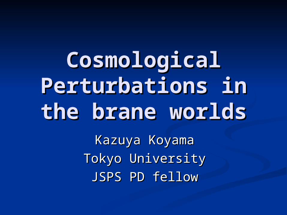
Cosmological Cosmological Perturbations in Perturbations in the brane worldsthe brane worlds
Kazuya KoyamaKazuya Koyama
Tokyo UniversityTokyo University
JSPS PD fellowJSPS PD fellow
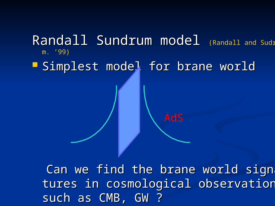
Randall Sundrum model Randall Sundrum model (Randall and Sudrum. ’99)
Simplest model for brane worldSimplest model for brane world
Can we find the brane world signatures in cosCan we find the brane world signatures in cos
mological observations such as CMB, GW ?mological observations such as CMB, GW ?
AdS
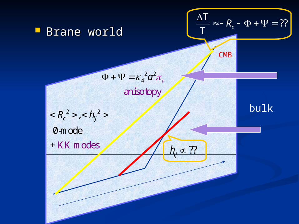
Brane worldBrane world
2 2,
0-mode
+ KK modes
c ijR h
2 24
anisotopy
a
CMB
T??
T cR
bulk
??ijh

Bulk inflaton modelBulk inflaton model Exact solutions for perturbationsExact solutions for perturbations
K.K. and K. Takahashi Phys. Rev. D 67 104011(2003)K.K. and K. Takahashi Phys. Rev. D 67 104011(2003) K.K. and K. Takahashi Phys. Rev. D in press (hep-th/03K.K. and K. Takahashi Phys. Rev. D in press (hep-th/03
07073)07073) Tensor perturbationsTensor perturbations Numerical calculationsNumerical calculations
H. Hiramatsu, K.K. and A. Taruya, H. Hiramatsu, K.K. and A. Taruya, Phys. Lett. B in press ( hep-th/0308072) Phys. Lett. B in press ( hep-th/0308072)
CMB anisotropies CMB anisotropies Low energy approximationLow energy approximation
T.Shiromizu and K.K. Phys. Rev. D 67 084022 (2003)T.Shiromizu and K.K. Phys. Rev. D 67 084022 (2003) K.K Phys. Rev. Lett. in press (astro-ph/0303108) K.K Phys. Rev. Lett. in press (astro-ph/0303108)
0-mode0-mode
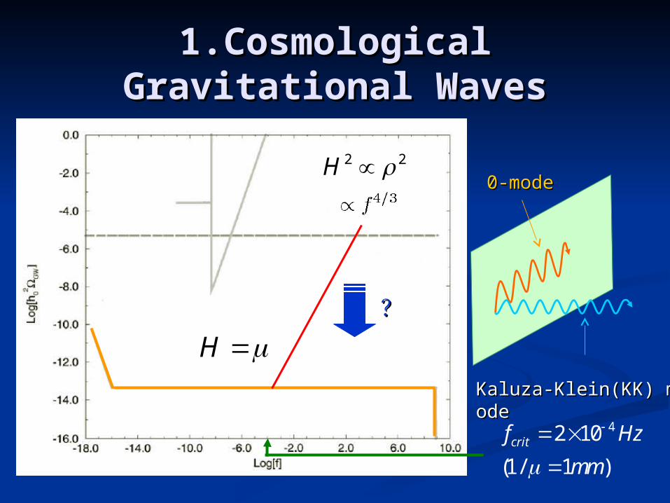
1.Cosmological 1.Cosmological Gravitational WavesGravitational Waves
Kaluza-Klein(KK) modeKaluza-Klein(KK) mode
??
2 2H
42 10
(1/ 1 )critf Hz
mm
H
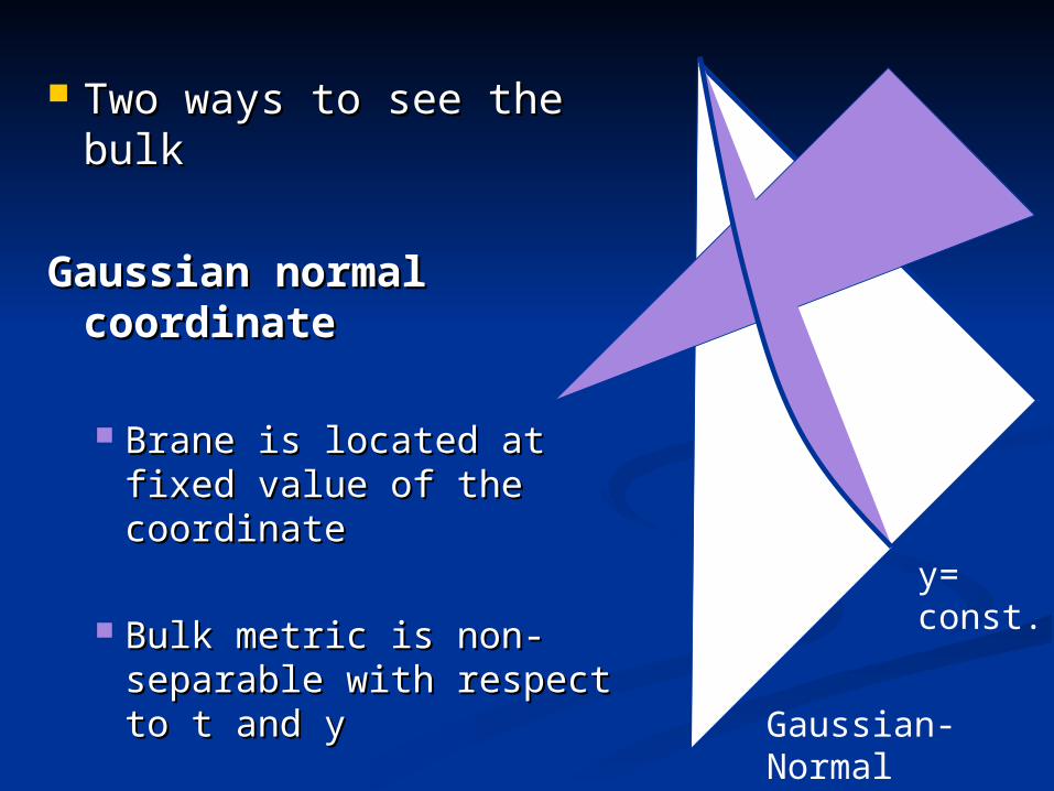
Two ways to see the Two ways to see the bulkbulk
Gaussian normal Gaussian normal coordinatecoordinate
Brane is located at fixed Brane is located at fixed
value of the coordinatevalue of the coordinate
Bulk metric is non-Bulk metric is non-separable with respect to separable with respect to t and yt and y
Gaussian-Normal coordinate
y= const.

Poincare coordinate
Static coordinateStatic coordinate
Bulk metric is Bulk metric is separable with respect separable with respect to t and y to t and y
Brane is moving Brane is moving
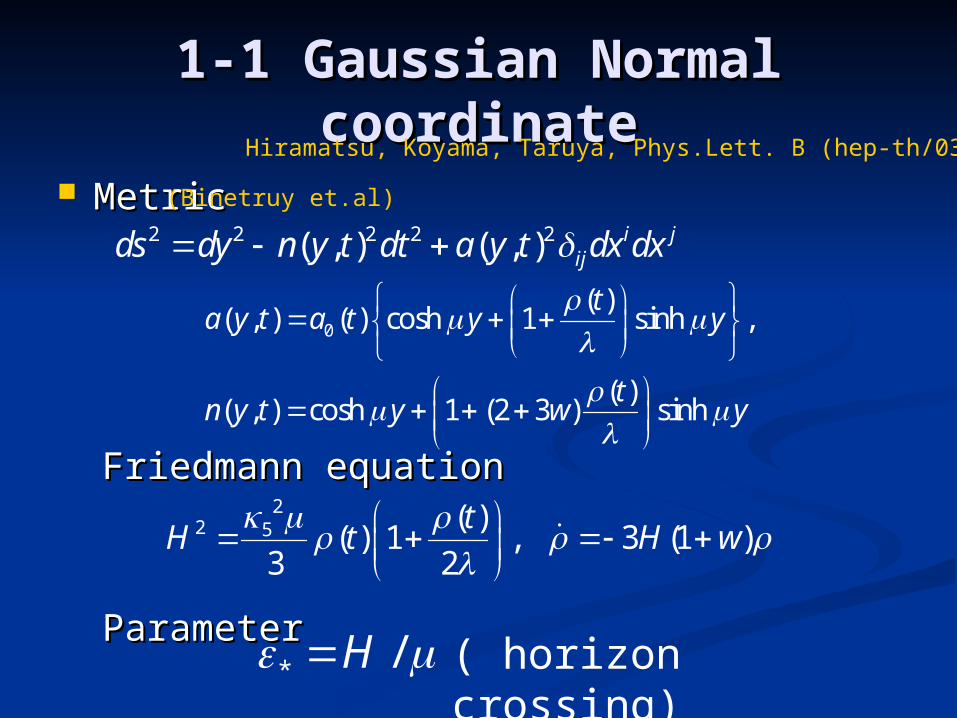
1-1 Gaussian Normal 1-1 Gaussian Normal coordinatecoordinate
MetricMetric
Friedmann equationFriedmann equation
Parameter Parameter
2 2 2 2 2( , ) ( , ) i jijds dy n y t dt a y t dx dx
0
( )( , ) ( ) cosh 1 sinh ,
( )( , ) cosh 1 (2 3 ) sinh
ta y t a t y y
tn y t y w y
22 5 ( )
( ) 1 , 3 (1 )3 2
tH t H w
Hiramatsu, Koyama, Taruya, Phys.Lett. B (hep-th/0308072)
* /H ( horizon crossing)
(Binetruy et.al)

Wave equationWave equation
Initial conditionInitial condition near brane/low energy metric is separablenear brane/low energy metric is separable 0-mode + KK-modes0-mode + KK-modes
No known brane inflation model predicts No known brane inflation model predicts significant significant
KK modes excitation during inflationKK modes excitation during inflation KK-modes are decreasing at super-horizon scales KK-modes are decreasing at super-horizon scales
We adopt 0-mode initial condition We adopt 0-mode initial condition at at
super-horizon scales ( h=const. ) super-horizon scales ( h=const. )
2 2 22 2
2 2 2
' '3 3 0,
h a n h n h a n hp h n
t a n t a y a n y
(Easther et. al., Battye et. al.)

Boundary conditionBoundary condition
There is a There is a coordinate singularitycoordinate singularity in the in the bulkbulk
y
t
( )cy y t
( )cy y t
( )cy y t
00y y
h
( )
0c ty y
n h
Physical brane
Regulator brane
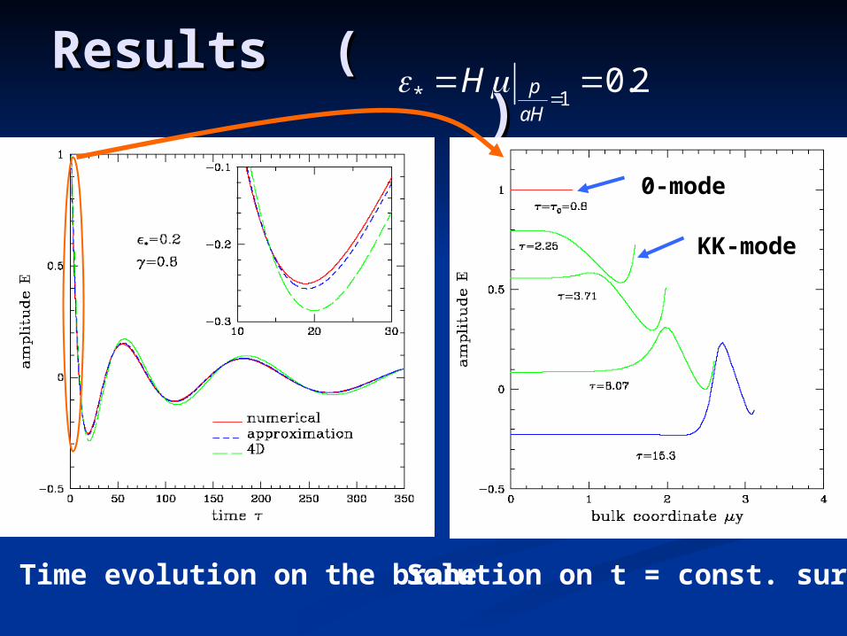
Results ( )Results ( )
Time evolution on the brane
KK-mode
0-mode
Solution on t = const. surface
* 10.2p
aH
H

Amplitude of GW decreases Amplitude of GW decreases due to KK modes excitationdue to KK modes excitation
suppression at ?suppression at ?damping
critf f
Damping factor 42 10critf Hz
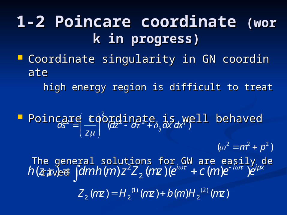
Coordinate singularity in GN coordinateCoordinate singularity in GN coordinate high energy region is difficult to treathigh energy region is difficult to treat
Poincare coordinate is well behaved Poincare coordinate is well behaved
The general solutions for GW are easily derivedThe general solutions for GW are easily derived
2
2 2 21( )i j
ijds dz d dx dxz
1-2 Poincare coordinate 1-2 Poincare coordinate (work in progres(work in progress)s)
22( , ) ( ) ( )( ( ) )i i ipxh z dmh m z Z mz e c m e e
(1) (2)2 2 2( ) ( ) ( ) ( )Z mz H mz b m H mz
2 2 2( )m p

Brane is movingBrane is moving
z
Motion of the brane
1, ( )
( )z T t
a t
2 22 5 ( )
( ) 13 2
a tH t
a
211 ( )
( )T H
a t
cosmic timethigh energy
low energy
2
( ) ( )2( , ) ( ) ( )
( ) ( )i T t i T tm
h t dm h m Z e c m ea t a t
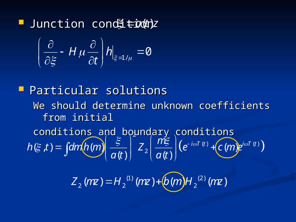
Junction conditionJunction condition
Particular solutionsParticular solutionsWe should determine unknown coefficients from We should determine unknown coefficients from
initialinitial
conditions and boundary conditions conditions and boundary conditions
( )a t z
1/0H h
t
(1) (2)2 2 2( ) ( ) ( ) ( )Z mz H mz b m H mz

Recovery of “0-mode” solutionRecovery of “0-mode” solution Due to the moving of the brane, “0-mode” on Due to the moving of the brane, “0-mode” on
FRW brane does NOT correspond to m=0 FRW brane does NOT correspond to m=0
Junction condition at late times Junction condition at late times
1/
4 42
2
( )22
2, log
( ) i T t
Ht
m i H m m mdm O
a a a a a
mh m Z e
a a
( ( ) )T t
Non-local terms
(“CFT” part in the context of AdS/CFT correspondence) 2 2
2
12 (1/ , ) 0p h t
a H

Numerical solution forNumerical solution for
Naïve boundary and initial conditions Naïve boundary and initial conditions “ “no incoming radiation” at Cauchy horizonno incoming radiation” at Cauchy horizon
Initial condition Initial condition
( )h m
2
(1) (1) ( )2
2
(2) (2) ( )2
( , ) ( )( ) ( )
( )( ) ( )
i T t
i T t
mh t dm h m H e
a t a t
mh m H e
a t a t
(1) ( ) (2) ( )( ) ( ) , ( , )im z im zdm h m e h m e m z
(1/ , ) 0, ( / 0)ih t p aH

Numerical results for low energyNumerical results for low energy
The resultant solution The resultant solution
20 40 60 80 100
-0.2
-0.1
0.1
0.2
0.3 Re[ ( )]h m
(1/ , )h t
/ 0.001H
( )i
m
a t 1
10 15 20 30 500.00001
0.0001
0.001
0.01
0.1
1
4D
4
1( ) ip
Dh t e
0( ) ipmh t e
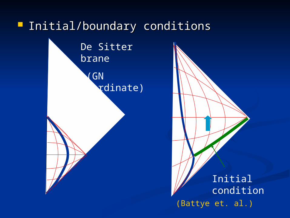
Initial/boundary conditionsInitial/boundary conditions
De Sitter brane
(GN coordinate)
Initial condition
(Battye et. al.)
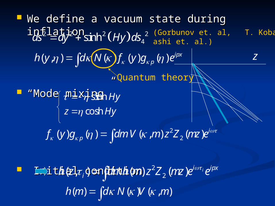
We define a vacuum state during inflation We define a vacuum state during inflation
““Mode mixing”Mode mixing”
Initial condition Initial condition
2 2 2 24sinhds dy Hy ds
( , ) ( ) ( ) ( ) ipxph y d N f y g e
22( ) ( ) ( , ) ( ) i
pf y g dm V m z Z mz e
sinh
cosh
Hy
z Hy
22( , ) ( ) ( ) ii ipx
ih z dmh m z Z mz e e ( ) ( ) ( , )h m d N V m
Quantum theory
(Gorbunov et. al, T. Kobayashi et. al.)
z
Prediction of GW at high Prediction of GW at high frequenciesfrequencies
(in the near future)(in the near future)
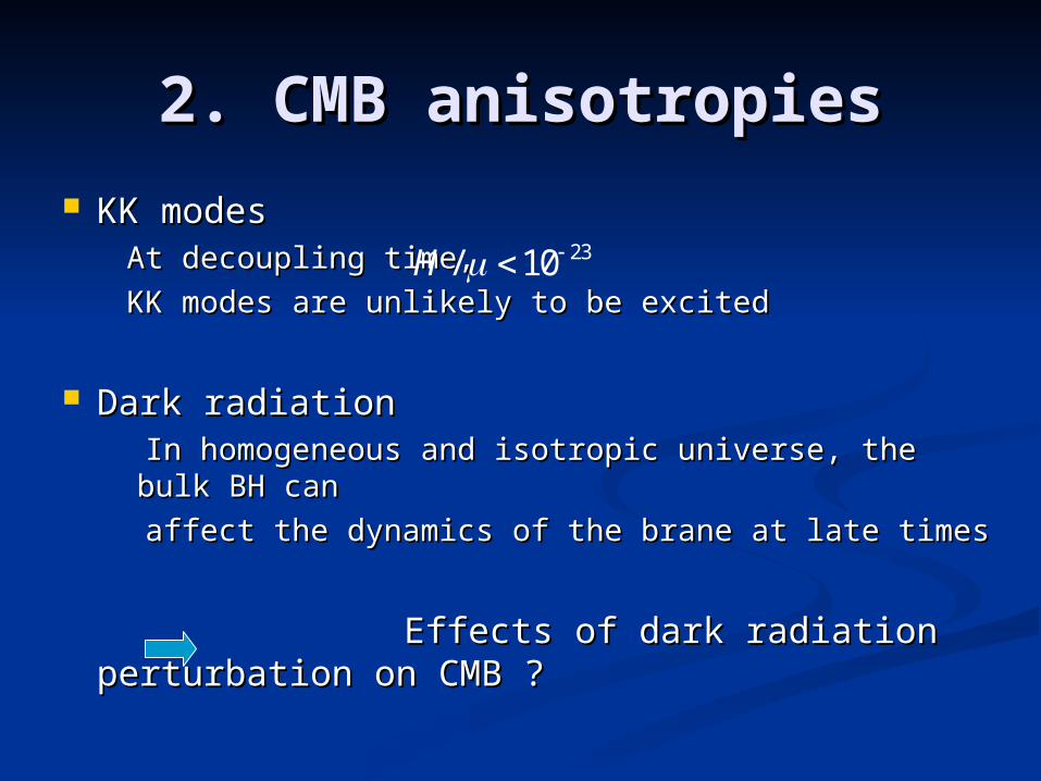
2. CMB anisotropies2. CMB anisotropies
KK modesKK modes At decoupling time,At decoupling time,
KK modes are unlikely to be excited KK modes are unlikely to be excited
Dark radiationDark radiation In homogeneous and isotropic universe, the bulk In homogeneous and isotropic universe, the bulk
BH can BH can
affect the dynamics of the brane at late timesaffect the dynamics of the brane at late times
Effects of dark radiation Effects of dark radiation perturbation on CMB ?perturbation on CMB ?
23/ 10H
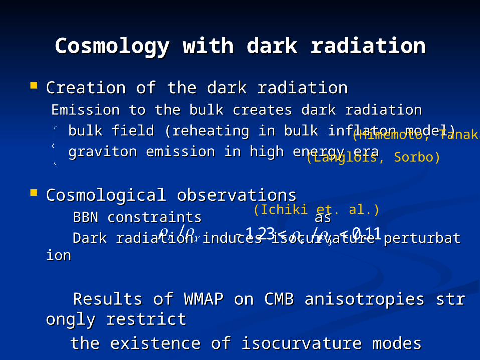
Cosmology with dark radiationCosmology with dark radiation
Creation of the dark radiationCreation of the dark radiationEmission to the bulk creates dark radiation Emission to the bulk creates dark radiation bulk field (reheating in bulk inflaton model)bulk field (reheating in bulk inflaton model) graviton emission in high energy eragraviton emission in high energy era
Cosmological observationsCosmological observations BBN constraints asBBN constraints as Dark radiation induces isocurvature perturbationDark radiation induces isocurvature perturbation
Results of WMAP on CMB anisotropies strongly reResults of WMAP on CMB anisotropies strongly restrictstrict
the existence of isocurvature modesthe existence of isocurvature modes
(Himemoto, Tanaka)
(Langlois, Sorbo)
/ 1.23 / 0.11 (Ichiki et. al.)

CMB anisotropies (SW effect)CMB anisotropies (SW effect)
for adiabatic perturbationfor adiabatic perturbation Longitudinal metric perturbationsLongitudinal metric perturbations
Curvature perturbationCurvature perturbation can be calculated can be calculated without solvingwithout solving
bulk perturbations but bulk perturbations but anisotropic stressanisotropic stress cannot becannot be
predicted unless bulk perturbations are knownpredicted unless bulk perturbations are known
m
T
T
2 1 2 2
,c
HR
H H
k a
Red shift
photonconst.m
(Langlois, Maartens, Sasaki, Wands)
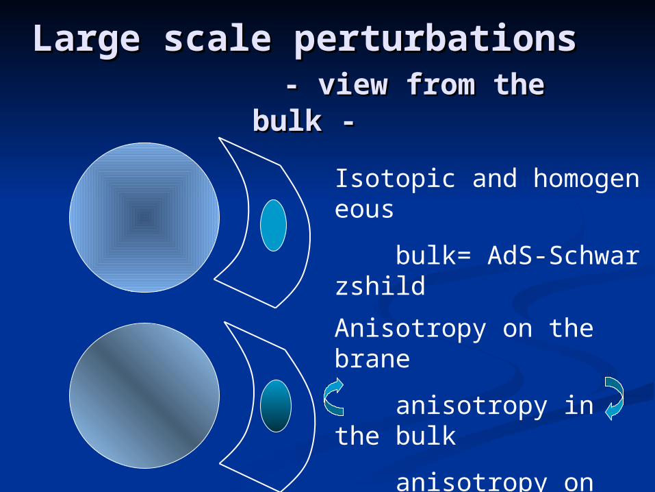
Large scale perturbationsLarge scale perturbations - view from the bulk -- view from the bulk -
Isotopic and homogeneous
bulk= AdS-Schwarzshild
Anisotropy on the brane
anisotropy in the bulk
anisotropy on the brane
Bulk and brane is coupled

Gaussian-Normal coordinate for Ads-SchwarzsGaussian-Normal coordinate for Ads-Schwarzshildhild
Consider the perturbation of dark radiationConsider the perturbation of dark radiation
2 2 2 2 2( , ) ( , ) i jijds dy n y t dt a y t dx dx
C C AdS spacetime + perturbations AdS spacetime + perturbations
2 2 2 2 2
2
ˆ1 2 ( , ) 2 ( , )
ˆ1 2 ( , ((1 2 ), ))
ii
i jij ij
ds dy n y t Y dt a B y t Y dx d
E y t
t
a y t Y Y dx dx
2 42
2 2 00 2 2
( , ) ( ) cosh(2 ) cosh(2 ) 1 1 sinh(2 )2
H CaHa y t a t y y y
2
2 450
( )( ) 1 ( )
3 2
tH t Ca t

Solutions for trace partSolutions for trace part
Equations for Equations for
1
2 2 40
2 22
1 ( / ) sinh(2 )ˆ ( , ) ,
2cosh( ) 1 ( / ) sinh( )
ˆ ˆ ˆ( , ) ( , ) ( , )
H y Cay t
y H y
ay t y t y t
a
2( ), ( )B O p E O p
2
2 2 2
' 'ˆˆ 2 " 5 ' 0,
' '" 3 ' 3
ˆ ˆ( ) 3
a a np B B
a a n
n a n aE E n E E
n a n a
n aa p n p B B
n a

In this gauge, the brane location is In this gauge, the brane location is perturbedperturbed
Perform infinitesimal coordinate Perform infinitesimal coordinate transformation and impose junction transformation and impose junction conditionsconditions
Matter perturbations

Junction condition relates matter Junction condition relates matter perturbation on the brane to and perturbation on the brane to and bulk perturbations bulk perturbations
Adiabatic condition on matter Adiabatic condition on matter perturbationsperturbations
equation for equation for
2 24 0
2 24 0 0
ˆ6 6 ' | ,
ˆ ˆ2 2 (2 3 ) ' | 2 ' |
y
y y
H H
P H H H
2 44 0Ca
2 44 0
1
3Ca
2sP c
2 2 2 2
2 2 44 0
(2 3 ) (3 2 3 )
1 1
2 3
s s
s
c H H H c H
c Ca
( 1)H
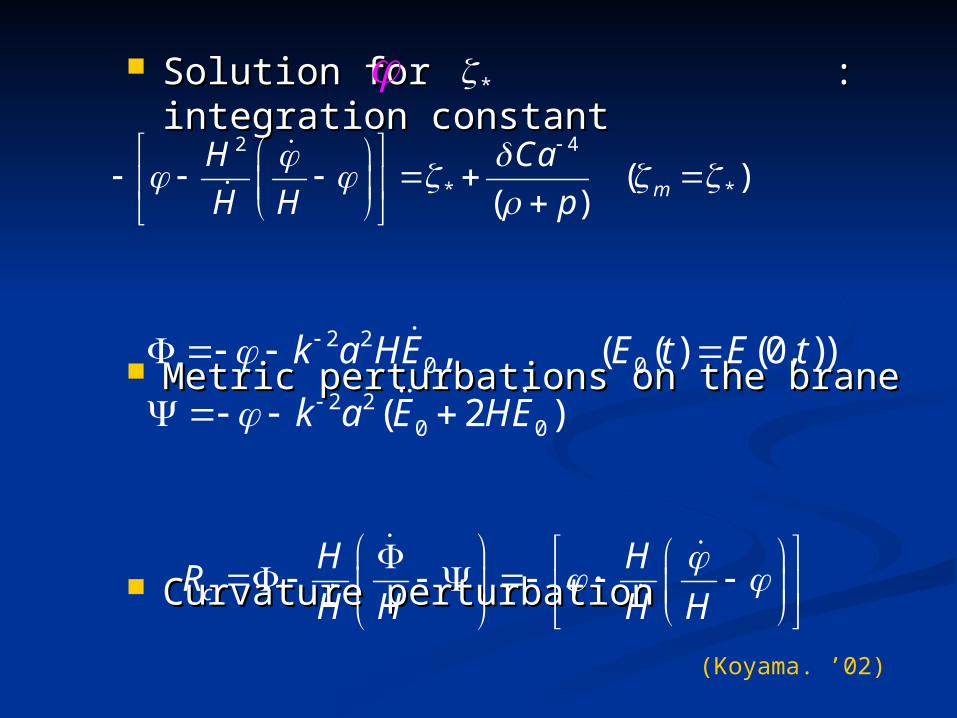
Solution for : integration Solution for : integration constant constant
Metric perturbations on the brane Metric perturbations on the brane
Curvature perturbationCurvature perturbation
2 4
* *( )( ) m
H Ca
H H p
*
2 20 0
2 20 0
, ( ( ) (0, ))
( 2 )
k a HE E t E t
k a E HE
c
H HR
H H H H
(Koyama. ’02)
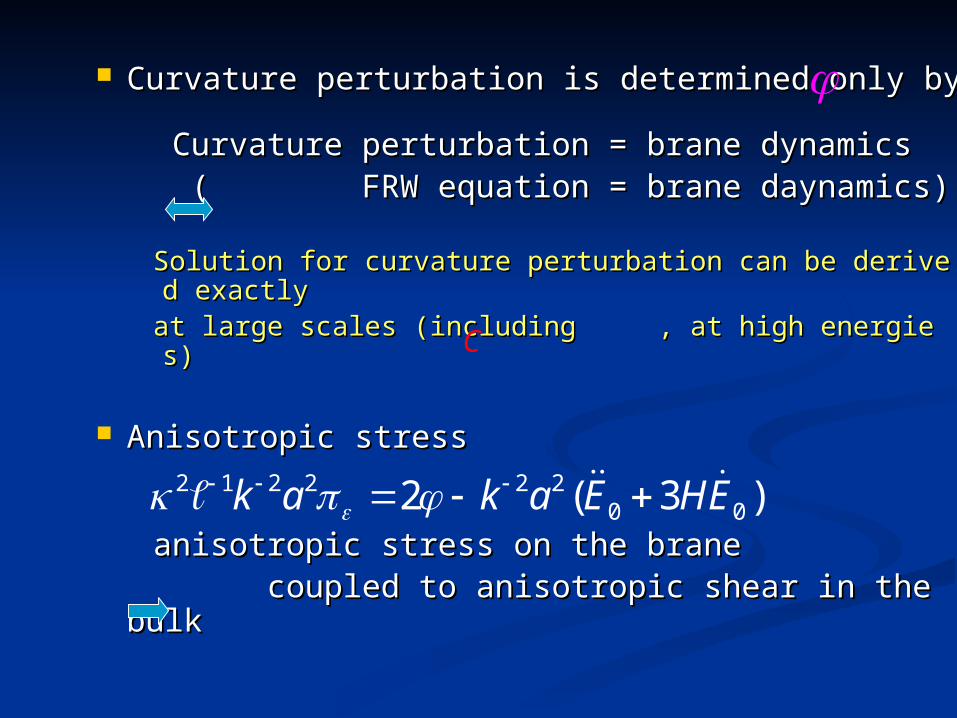
Curvature perturbation is determined only by Curvature perturbation is determined only by
Curvature perturbation = brane dynamicsCurvature perturbation = brane dynamics ( FRW equation = brane daynamics)( FRW equation = brane daynamics)
Solution for curvature perturbation can be derived exactly Solution for curvature perturbation can be derived exactly at large scales (including , at high energies)at large scales (including , at high energies)
Anisotropic stressAnisotropic stress
anisotropic stress on the braneanisotropic stress on the brane coupled to anisotropic shear in the bulk coupled to anisotropic shear in the bulk
2 1 2 2 2 20 02 ( 3 )k a k a E HE
C
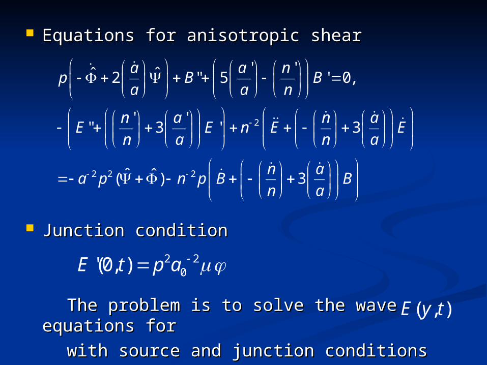
Equations for anisotropic shearEquations for anisotropic shear
Junction conditionJunction condition
The problem is to solve the wave The problem is to solve the wave equations for equations for
with source and junction conditions with source and junction conditions
2
2 2 2
' 'ˆˆ 2 " 5 ' 0,
' '" 3 ' 3
ˆ ˆ( ) 3
a a np B B
a a n
n a n aE E n E E
n a n a
n aa p n p B B
n a
2 20'(0, )E t p a
( , )E y t
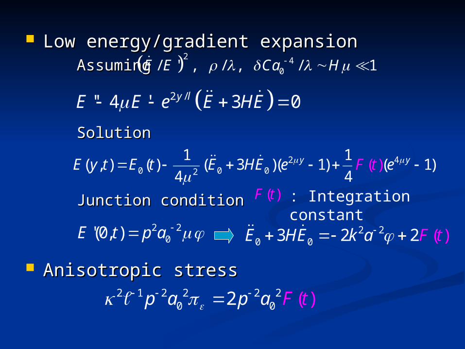
Low energy/gradient expansion Low energy/gradient expansion AssumingAssuming
Solution Solution
Junction condition Junction condition
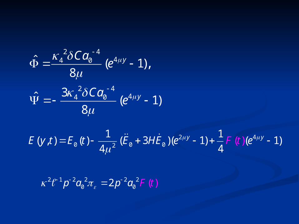
Anisotropic stressAnisotropic stress
2 40/ ' , / , / 1E E Ca H
2 /'' 4 ' 3 0y lE E e E HE
2 40 0 02
1 1( , ) ( ) ( 3 )( 1) ( 1)
4)
4(y yE y t E t E HE F te e
( )F t : Integration constant
2 20 03 2 ( )2E HE k a F t 2 2
0'(0, )E t p a
2 1 2 2 2 20 0 ( )2p a F tp a
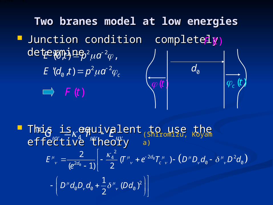
Junction condition completely determine Junction condition completely determine
This is equivalent to use the effective theoryThis is equivalent to use the effective theory
4 ( , )d y xE e e
0
0
22 24
0 02
20 0 0
2( )
( 1) 2
1( )
2
dcdE T e T D D d D d
e
D d D d Dd
(Shiromizu, Koyama)
( )t ( )c t0d
2 2
2 20
'(0, ) ,
'( , ) c
E t p a
E d t p a
( )F t
(4) 24G T E
( )F t
Two branes model at low energiesTwo branes model at low energies
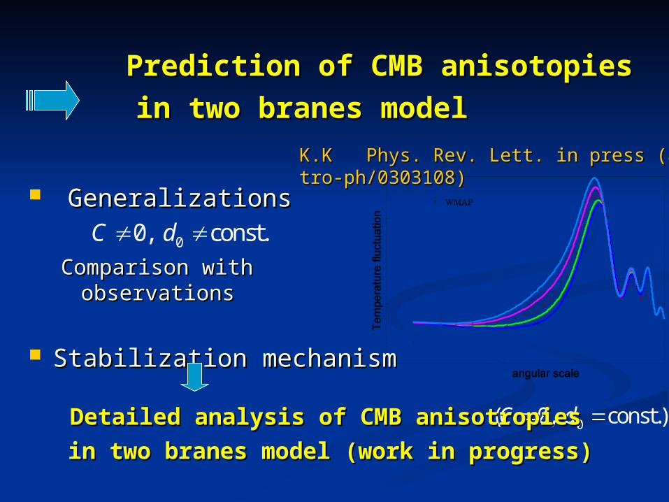
Prediction of CMB anisotopiesPrediction of CMB anisotopies in two branes modelin two branes model
K.K Phys. Rev. Lett. in press (astro-ph/030310K.K Phys. Rev. Lett. in press (astro-ph/0303108)8)
0( 0, const.)C d Detailed analysis of CMB anisotropiesDetailed analysis of CMB anisotropies in two branes model (work in progress)in two branes model (work in progress)
GeneralizationsGeneralizations
Comparison with observationsComparison with observations
Stabilization mechanismStabilization mechanism
00, const.C d
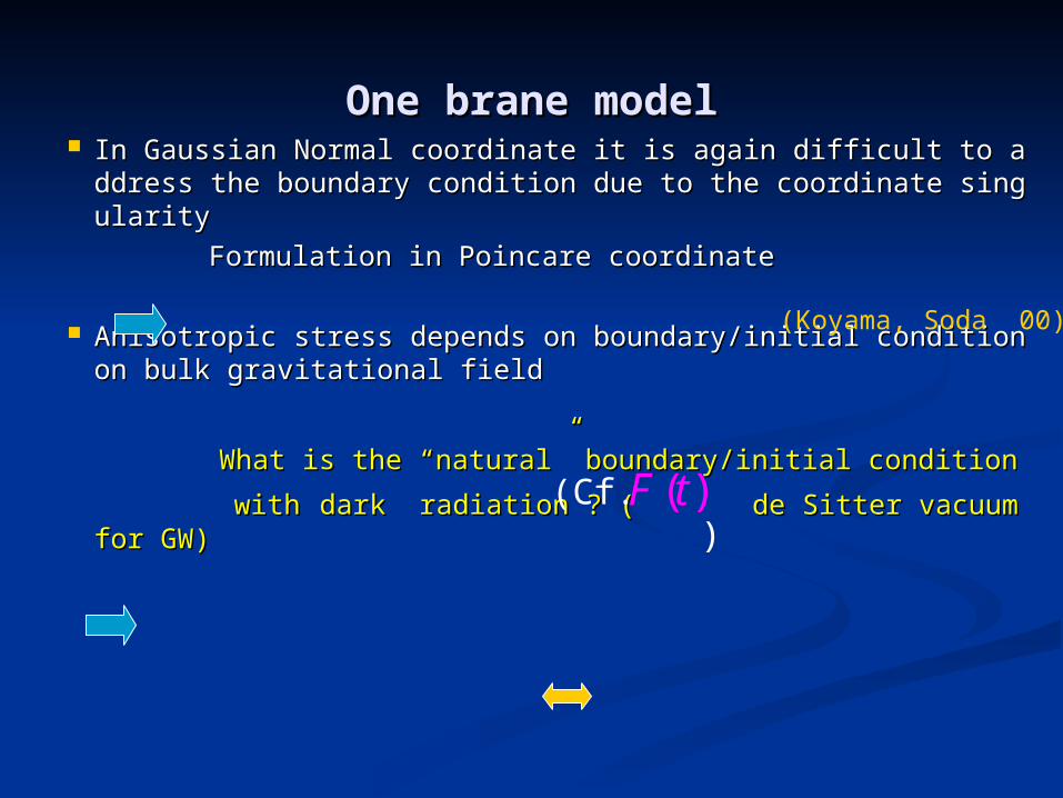
In Gaussian Normal coordinate it is again difficult to address thIn Gaussian Normal coordinate it is again difficult to address the boundary condition due to the coordinate singularity e boundary condition due to the coordinate singularity
Formulation in Poincare coordinateFormulation in Poincare coordinate
Anisotropic stress depends on boundary/initial condition on bulAnisotropic stress depends on boundary/initial condition on bulk gravitational fieldk gravitational field
What is the “natural” boundary/initial condition What is the “natural” boundary/initial condition
withwith dark radiation ? ( de Sitter vacuum for GW)dark radiation ? ( de Sitter vacuum for GW)
One brane modelOne brane model
(Koyama, Soda 00)
( )F t(Cf. )

We should understand the relation between the We should understand the relation between the choice of the boundary condition in the bulk andchoice of the boundary condition in the bulk and the behavior of anisotropic stress on the branethe behavior of anisotropic stress on the brane
Anisotropic stress boundary conditionAnisotropic stress boundary condition
NumericallyNumerically Toy model where this relation can beToy model where this relation can be analytically examined in a whole bulk spacetimeanalytically examined in a whole bulk spacetime
(Koyama, Takahashi, hep-th/0307073)
2 444 0
2 444 0
ˆ ( 1),8
3ˆ ( 1)8
y
y
Cae
Cae
2 40 0 02
1 1( , ) ( ) ( 3 )( 1) ( 1)
4)
4(y yE y t E t E HE F te e
2 1 2 2 2 20 0 ( )2p a F tp a


![HANIWA — koyama M's House AË+igweek] s 77 HAPPY KURA …](https://img.pdfslide.tips/doc/110x75/623f5cc20eab0f781715ed3a/haniwa-koyama-ms-house-aigweek-s-77-happy-kura-.jpg)