Embed Size (px)
Citation preview
Cost Assessment of Cellulosic Ethanol Production and Distribution in the US
William R MorrowW. Michael GriffinH. Scott Matthews
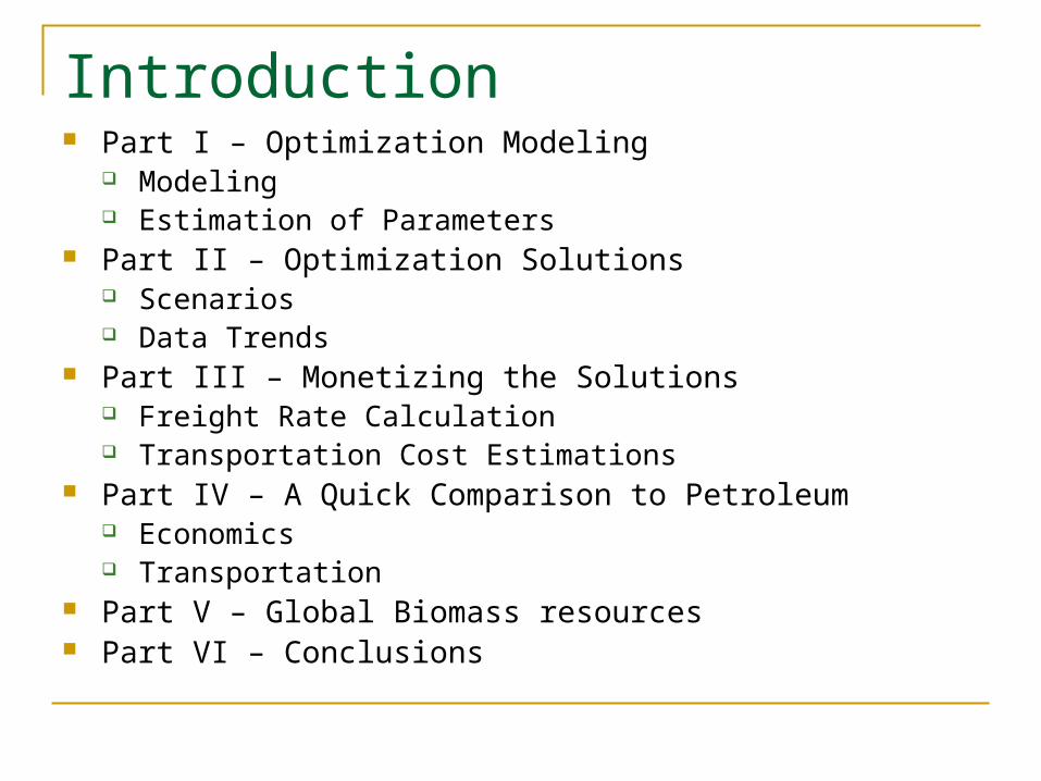
Introduction Part I – Optimization Modeling
Modeling Estimation of Parameters
Part II – Optimization Solutions Scenarios Data Trends
Part III – Monetizing the Solutions Freight Rate Calculation Transportation Cost Estimations
Part IV – A Quick Comparison to Petroleum Economics Transportation
Part V – Global Biomass resources Part VI – Conclusions
Part I – Optimization Modeling (Modeling)
Estimate an Extended Corn Based Ethanol Scenario
Model domestic switchgrass energy crop (published data) as the feedstock for cellulosic ethanol production
Estimate transportation costs as domestic cellulosic ethanol production increases
Identify any capacity limitations for a switchgrass based cellulosic ethanol fuel economy
Modeling Goals
Part I – Optimization Modeling (Modeling)
Distributes ethanol to MSAs Capable of large blend ratios Expands corn production as far as believable
& makes up remaining required ethanol with switchgrass based cellulosic ethanol
Only considers truck and rail and transport Uses freight rates derived from US Economic
Input Output data, and Commodity Flow Survey
Our Model
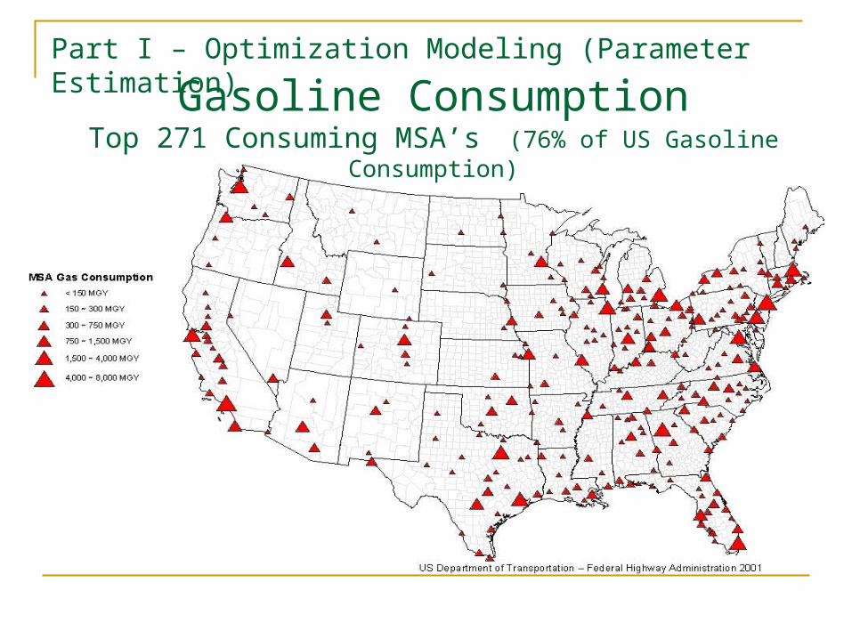
Part I – Optimization Modeling (Parameter Estimation)Gasoline Consumption
Top 271 Consuming MSA’s (76% of US Gasoline Consumption)
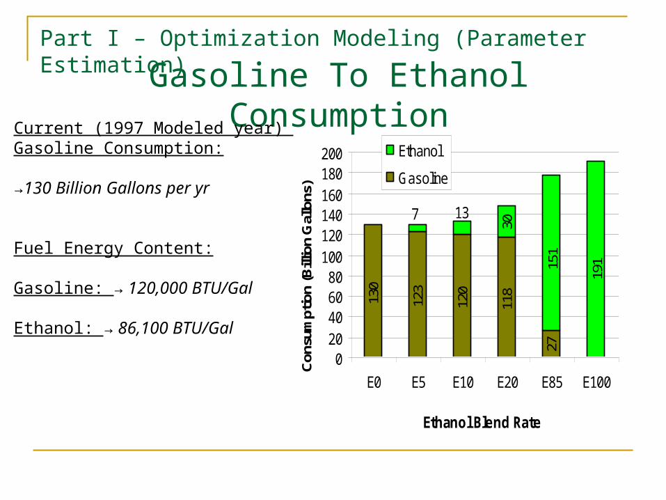
Part I – Optimization Modeling (Parameter Estimation)Gasoline To Ethanol ConsumptionCurrent (1997 Modeled year) Gasoline Consumption:
→130 Billion Gallons per yr
Fuel Energy Content:
Gasoline: → 120,000 BTU/Gal
Ethanol: → 86,100 BTU/Gal
123
120
118
27
130
7 13
30
151
191
020406080
100120140160180200
E0 E5 E10 E20 E85 E100
Ethanol Blend Rate
Con
sum
ptio
n (B
illio
n G
allo
ns)
Ethanol
Gasoline
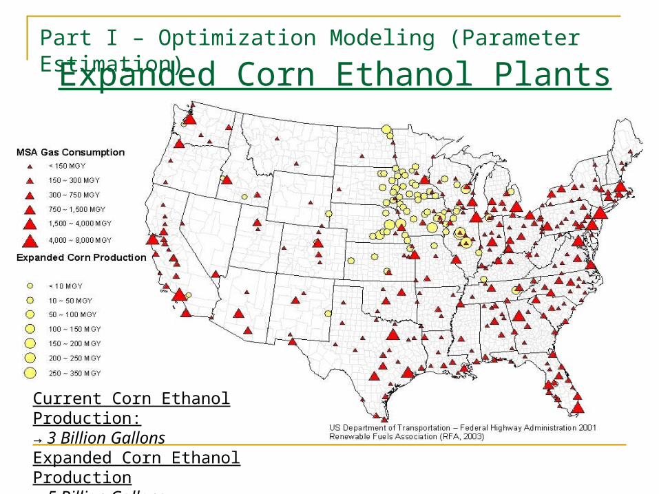
Part I – Optimization Modeling (Parameter Estimation)Expanded Corn Ethanol Plants
Current Corn Ethanol Production:→ 3 Billion GallonsExpanded Corn Ethanol Production→ 5 Billion Gallons
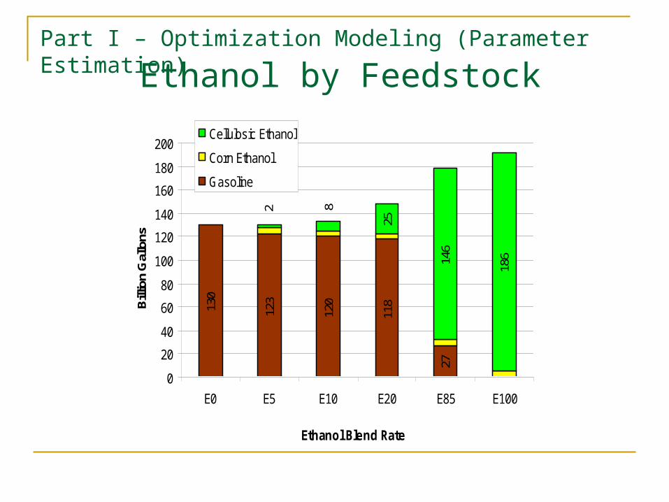
Part I – Optimization Modeling (Parameter Estimation)Ethanol by Feedstock
130
123
120
118
27
25
146
186
82
0
20
40
60
80
100
120
140
160
180
200
E0 E5 E10 E20 E85 E100
Ethanol Blend Rate
Bill
ion
Gal
lons
Cellulosic Ethanol
Corn Ethanol
Gasoline
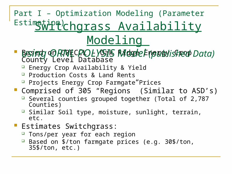
Part I – Optimization Modeling (Parameter Estimation)
Based on ORECCL – Oak Ridge Energy Crop County Level Database Energy Crop Availability & Yield Production Costs & Land Rents Projects Energy Crop Farmgate Prices
Comprised of 305 “Regions” (Similar to ASD’s) Several counties grouped together (Total of 2,787
Counties) Similar Soil type, moisture, sunlight, terrain, etc.
Estimates Switchgrass: Tons/per year for each region Based on $/ton farmgate prices (e.g. 30$/ton, 35$/ton, etc.)
Switchgrass Availability Modeling
using ORNL POLYSIS Model (published Data)
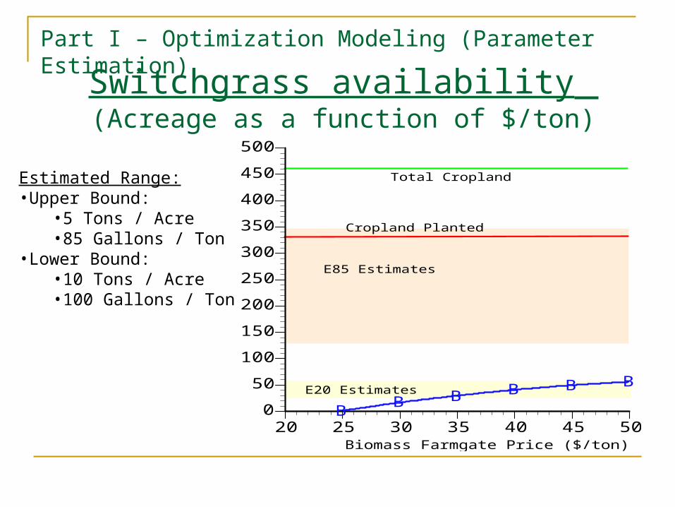
Part I – Optimization Modeling (Parameter Estimation)
Switchgrass availability (Acreage as a function of $/ton)
BB B B B B
0
50
100
150
200
250
300
350
400
450
500
20 25 30 35 40 45 50
Sw
itch
gra
ss P
lan
ted
(m
illio
n a
cre
s)
Biomass Farmgate Price ($/ton)
Total Cropland
Cropland Planted
E85 Estimates
E20 Estimates
Estimated Range:•Upper Bound:
•5 Tons / Acre•85 Gallons / Ton
•Lower Bound:•10 Tons / Acre•100 Gallons / Ton
Part I – Optimization Modeling (Parameter Estimation)Transforming Switchgrass into
Ethanol Gallons
Minimum plant size of 2,200 Ton SWG/day based on the work of Wooley et al. (1999, 1999a)
85 Gallons / Ton SWG (from range of 68 ~ 100 Gallons / Ton SWG) based on the work of Wooley et al. (1999, 1999a)
Question: Can a POLYSIS Region produce enough SWG to support the minimum plant requirement? At what price ($ / Ton SWG)?
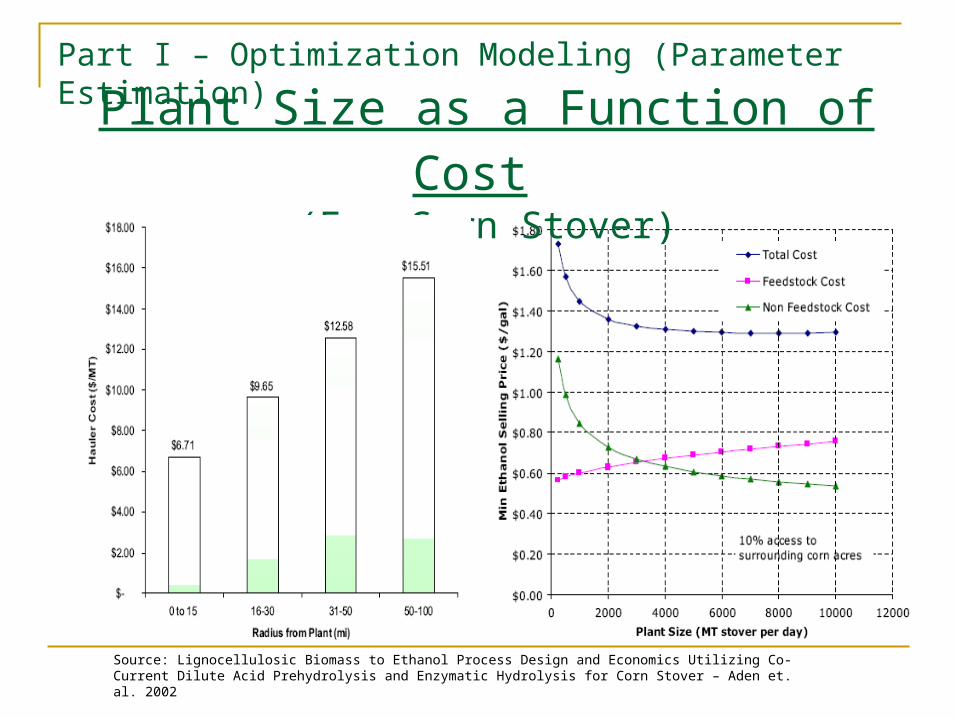
Part I – Optimization Modeling (Parameter Estimation)
Plant Size as a Function of Cost (For Corn Stover)
Source: Lignocellulosic Biomass to Ethanol Process Design and Economics Utilizing Co-Current Dilute Acid Prehydrolysis and Enzymatic Hydrolysis for Corn Stover – Aden et. al. 2002
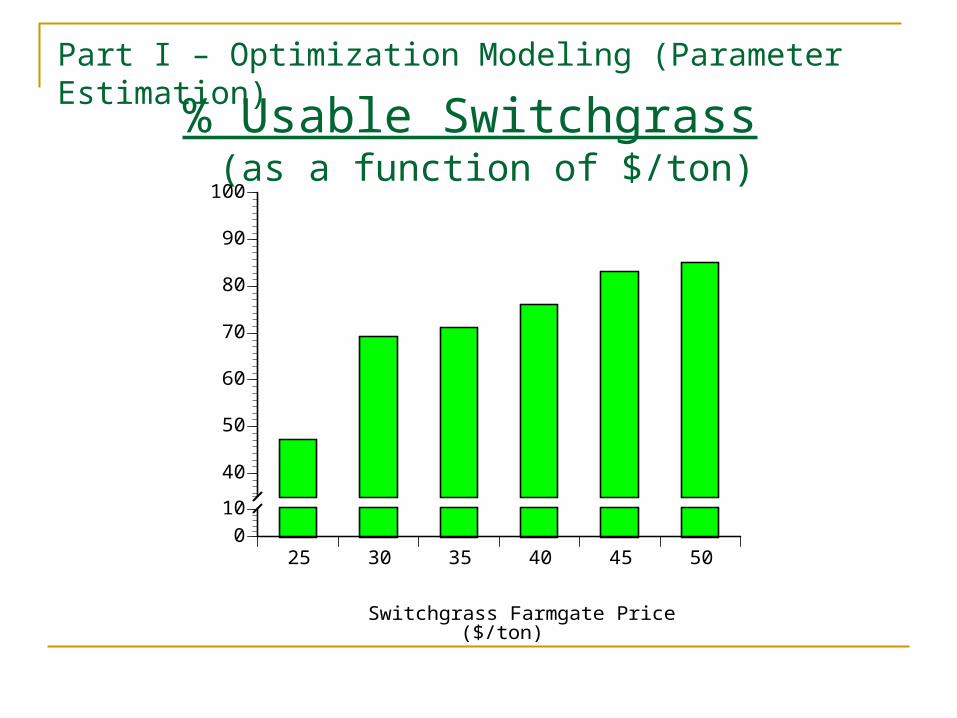
Part I – Optimization Modeling (Parameter Estimation)
% Usable Switchgrass (as a function of $/ton)
25 30 35 40 45 500
10
40
50
60
70
80
90
100
Ava
ilab
le S
witc
hg
rass
(%
of T
ota
l Pro
du
ced
)
Switchgrass Farmgate Price ($/ton)
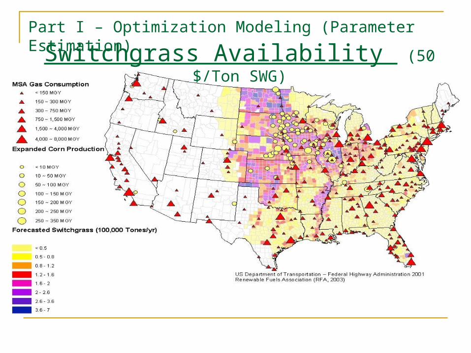
Part I – Optimization Modeling (Parameter Estimation)Switchgrass Availability (50 $/Ton
SWG)
Part II – Optimization Solutions (Scenarios)
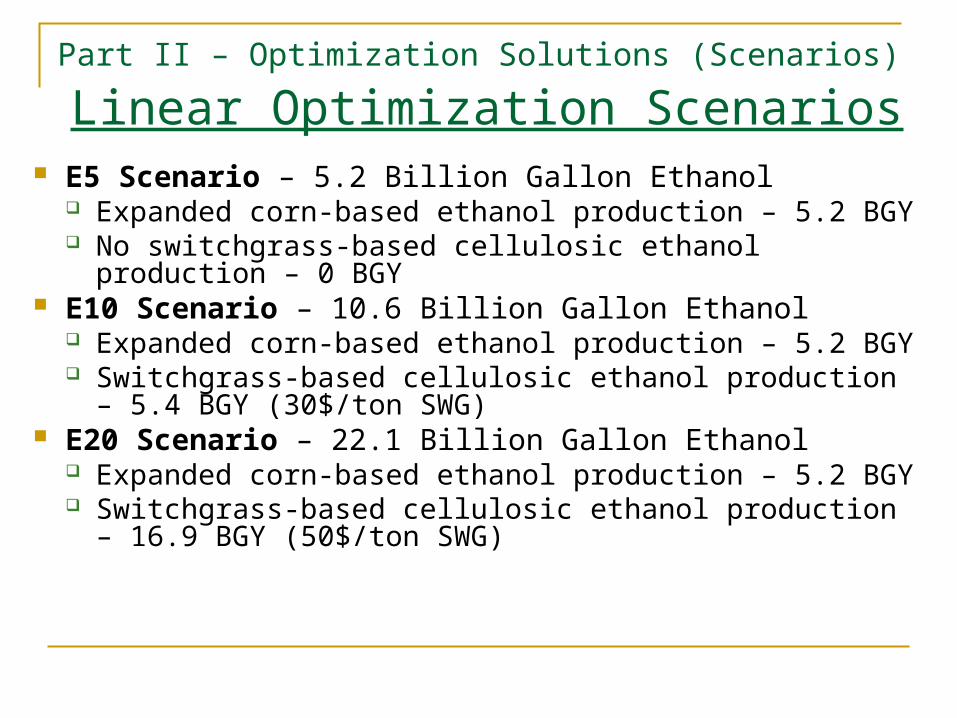
Linear Optimization Scenarios E5 Scenario – 5.2 Billion Gallon Ethanol
Expanded corn-based ethanol production – 5.2 BGY No switchgrass-based cellulosic ethanol production – 0
BGY E10 Scenario – 10.6 Billion Gallon Ethanol
Expanded corn-based ethanol production – 5.2 BGY Switchgrass-based cellulosic ethanol production – 5.4
BGY (30$/ton SWG) E20 Scenario – 22.1 Billion Gallon Ethanol
Expanded corn-based ethanol production – 5.2 BGY Switchgrass-based cellulosic ethanol production – 16.9
BGY (50$/ton SWG)
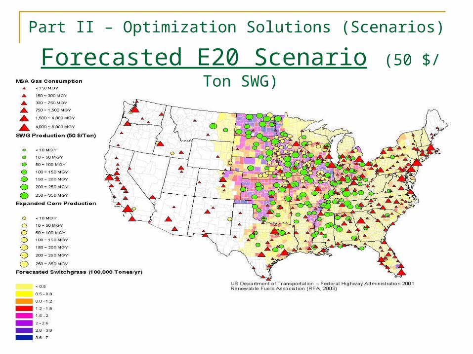
Part II – Optimization Solutions (Scenarios)
Forecasted E20 Scenario (50 $/ Ton SWG)
Part I – Optimization Modeling (Modeling)
1 1
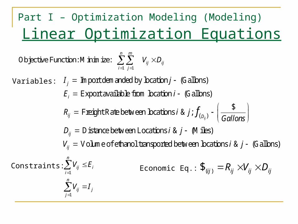
Objective Function: Minimize: n m
ij iji j
V D
Import demanded by location (Gallons)
Export available from location (Gallons)
$ Freight Rate between locations & ;
Distance between Locations & (Miles)
ij
j
i
ij D
ij
ij
I j
E i
R i jGallons
D i j
V
f
Volume of ethanol transported between locations & (Gallons)i j
1
1
n
ij ii
n
ij jj
V E
V I
Linear Optimization Equations
Variables:
Constraints: Economic Eq.: ( )$ ij ij ij ijR V D
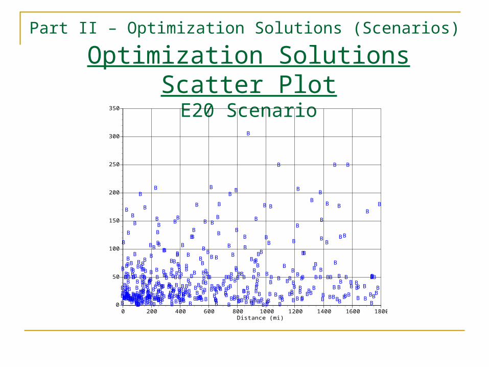
Part II – Optimization Solutions (Scenarios)
Optimization Solutions Scatter Plot
E20 Scenario
BB
B
B
B
B
BBBB
B
BB
B
BBB
B
BB
B
B
B
BBBBBBBB
B
B
B
B
BB
B
BB
B
BBB
BBBB
B
BB
BB
B
B
B
BB
BB
BBBB
B
B
B
BBBBBBB
BB
B
B
B
B
BB
BB
B
BB
BBB
B
BB
B
B
B
BBBB
B
BB
B
B
B
B
BB
B
BBBB
B
B
B
B
B
BBBB
B
B
BBBBBB
B
B
B
BBB
B
B
B
BB
B
B
BBB
B
BBBB
B
B
B
B
B
B
B
B
B
B
B
B
B
B
BB
B
B
B
B
BB
BB
B
BB
BBB
B
B
B
B
B
BB
BB
BB
B
BB
B
B
B
B
B
BBB
B
BBBB
B
B
B
B
B
B
B
B
B
B
B
BBB
B
B
B
B
B
B
B
B
B
B
B
BBBBBBBBB
BB
B
B
B
BBB
BB
B
B
BB
B
B
B
B
BBB
B
B
B
BB
B
B
B
B
B
B
B
B
B
B
B
B
BB
B
BB
B
B
B
B
B
BB
BB
B
B
B
B
B
B
B
B
B
BBBB
BB
B
BB
B
B
B
B
BB
B
B
B
BB
B
B
BB
B
B
B
B
B
BB
B
B
B
B
B
B
B
B
B
BB
B
B
B
BB
B
B
B
B
B
B
B
BBBB
B
B
B
B
BB
B
BB
B
B
B
BBB
B
B
B
BB
B
B
B
BBBB
B
B
B
B
BB
B
B
B
B
B
B
B
B
B
BB
B
BB
B
BB
BBB
B
B
BB
B
B
BB
B
B
BB
B
B
B
B
B
B
B
B
B
B
B
B
B
B
B
B
B
B
B
B
B
B
BB
BB
B
B B
B
B
B
B
BBB
B
B
BB
B
0
50
100
150
200
250
300
350
0 200 400 600 800 1000 1200 1400 1600 1800
Vo
lum
e (
mill
ion
ga
llon
s)
Distance (mi)
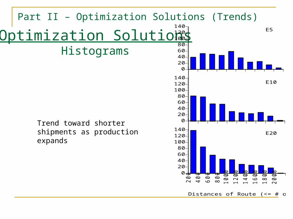
Part II – Optimization Solutions (Trends)
Optimization SolutionsHistograms
20
0
40
0
60
0
80
0
10
00
12
00
14
00
16
00
18
00
20
000
20406080
100120140
Distances of Route (<= # of miles)
020406080
100120140
Nu
mb
er
of
Ro
ute
s
020406080
100120140
E5
E10
E20
Trend toward shorter shipments as production expands
Part III – Monetizing the Solutions (Freight Rate Estimation)Freight Rate Dilemma
Problem: Freight industry does not publishes freight rates directly
Solution: Use US Government data sources and extrapolate freight rates
Data sources: US Department of Commerce; Bureau of
Economic Analysis – Input ~ Output Accounts US Department of Transportation; Commodity
Flow Survey
Part III – Monetizing the Solutions (Freight Rate Estimation)Freight Rate Estimation Method EIO Accounts:
Use of Commodities by Industry 1997 – Total Commodity Output. IO Code 482000 – Truck Transportation IO Code 244000 – Rail Transportation
CFS Database: Shipment by Destination and Mode of Transport
1997 Truck Rail
US State to State Distance matrix
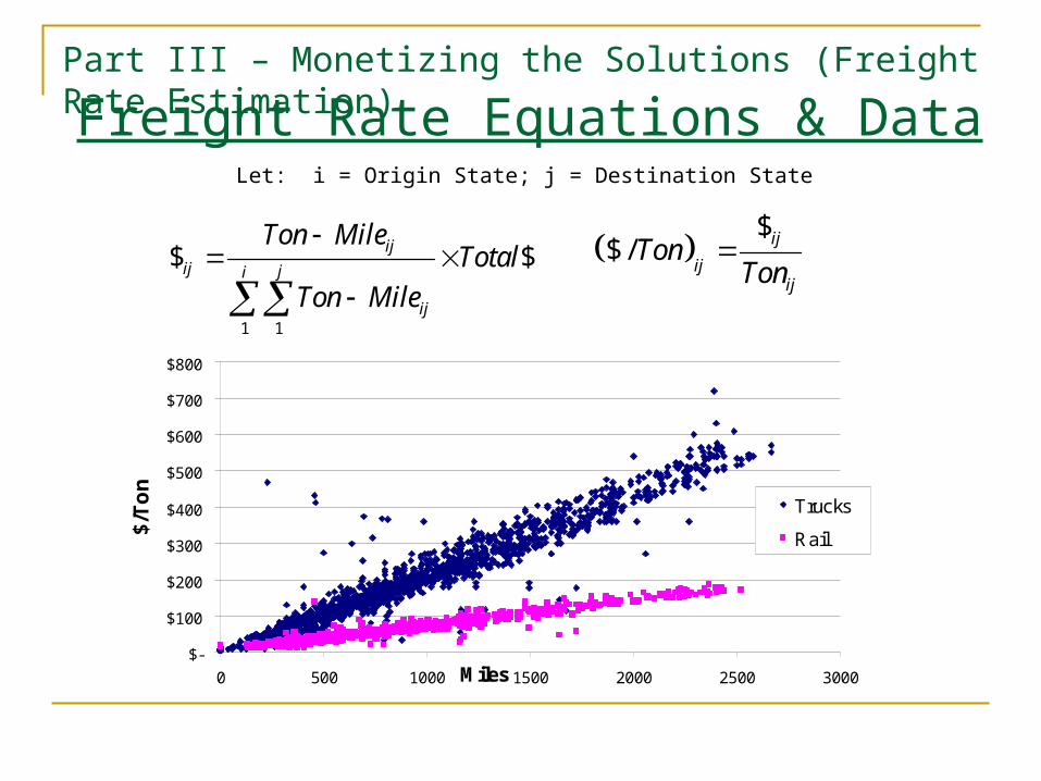
Part III – Monetizing the Solutions (Freight Rate Estimation)
1 1
$ $ijij ji
ij
Ton MileTotal
Ton Mile
Freight Rate Equations & Data
$-
$100
$200
$300
$400
$500
$600
$700
$800
0 500 1000 1500 2000 2500 3000Miles
$/T
on
Trucks
Rail
$
$ / ij
ijij
TonTon
Let: i = Origin State; j = Destination State
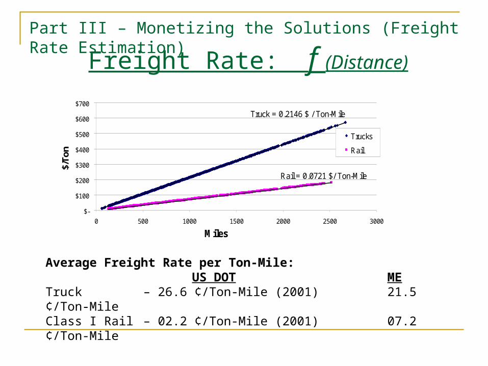
Part III – Monetizing the Solutions (Freight Rate Estimation)
Freight Rate: f (Distance)
Truck = 0.2146 $ / Ton-Mile
Rail = 0.0721 $/ Ton-Mile
$-
$100
$200
$300
$400
$500
$600
$700
0 500 1000 1500 2000 2500 3000
Miles
$/To
n
Trucks
Rail
Average Freight Rate per Ton-Mile:US DOT ME
Truck – 26.6 ¢/Ton-Mile (2001) 21.5 ¢/Ton-Mile Class I Rail – 02.2 ¢/Ton-Mile (2001) 07.2 ¢/Ton-Mile
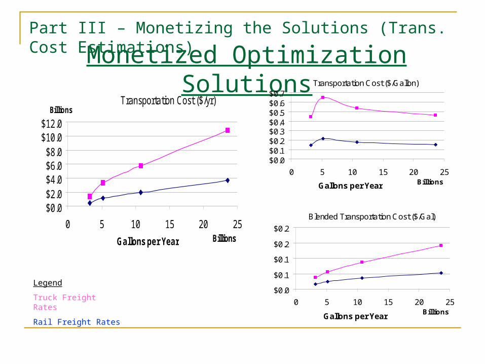
Part III – Monetizing the Solutions (Trans. Cost Estimations)Monetized Optimization Solutions
Transportation Cost ($/yr)
$0.0$2.0$4.0$6.0$8.0
$10.0$12.0
0 5 10 15 20 25
Billions
BillionsGallons per Year
Transportation Cost ($/Gallon)
$0.0$0.1$0.2$0.3$0.4$0.5$0.6$0.7
0 5 10 15 20 25BillionsGallons per Year
Blended Transportation Cost ($/Gal)
$0.0
$0.1
$0.1
$0.2
$0.2
0 5 10 15 20 25BillionsGallons per Year
Legend
Truck Freight Rates
Rail Freight Rates
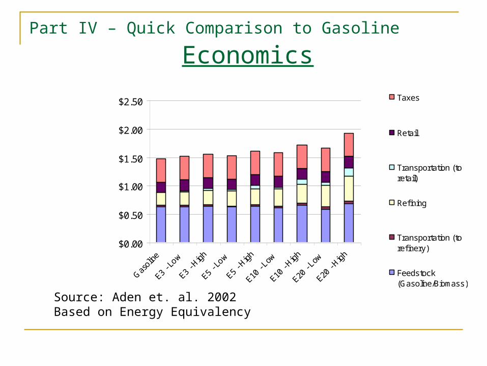
Part IV – Quick Comparison to Gasoline
Economics
$0.00
$0.50
$1.00
$1.50
$2.00
$2.50
Gas
oline
E3 - L
ow
E3 - H
igh
E5 - L
ow
E5 - H
igh
E10 -
Low
E10 -
High
E20 -
Low
E20 -
High
Taxes
Retail
Transportation (toretail)
Refining
Transportation (torefinery)
Feedstock(Gasoline/Biomass)
Source: Aden et. al. 2002Based on Energy Equivalency
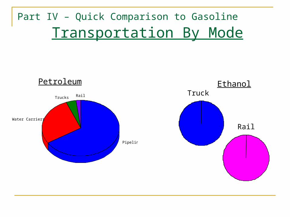
Part IV – Quick Comparison to Gasoline
Transportation By Mode
Pipelines
Water Carriers
Trucks Rail
Petroleum EthanolTruck
Rail
Part IV – Quick Comparison to Gasoline
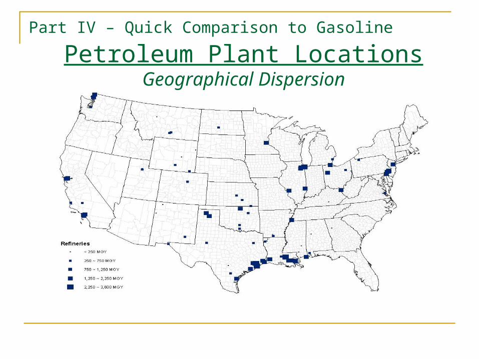
Petroleum Plant LocationsGeographical Dispersion
Part IV – Quick Comparison to Gasoline
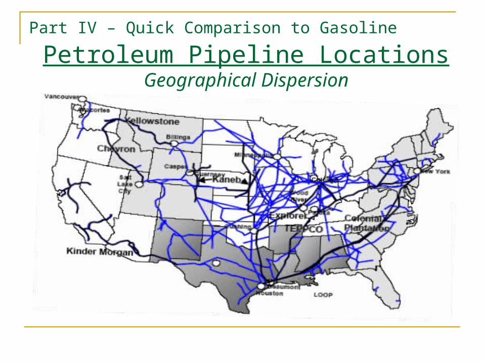
Petroleum Pipeline LocationsGeographical Dispersion
Part IV – Quick Comparison to Gasoline
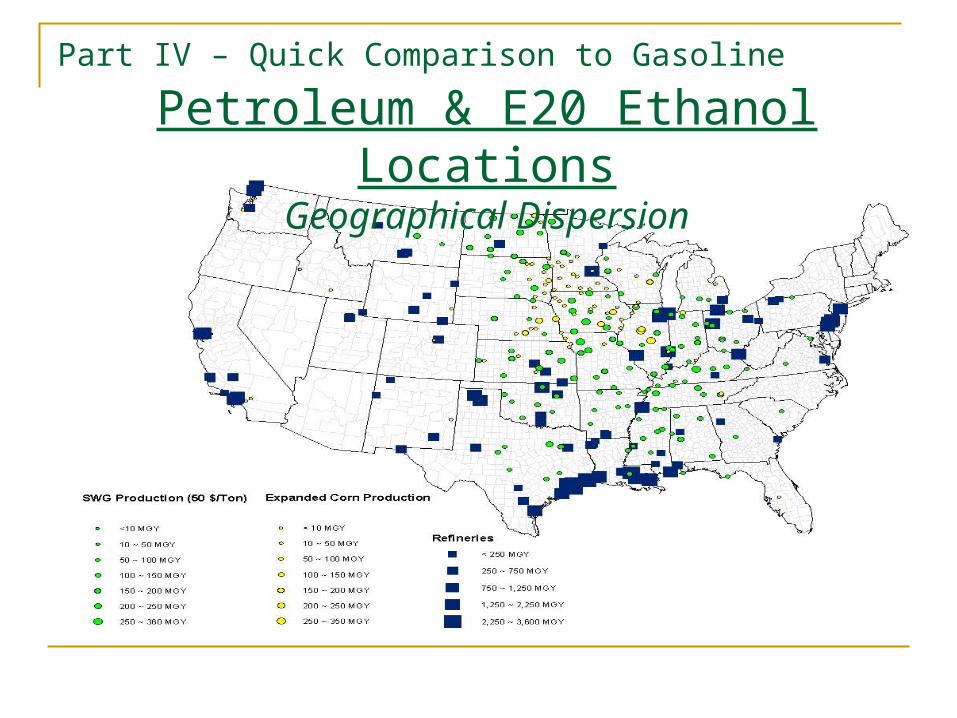
Petroleum & E20 Ethanol Locations
Geographical Dispersion
Part IV – Quick Comparison to Gasoline
Can not ship ethanol in petroleum pipelines Location of ethanol production is more widely
distributed than refineries locations Ethanol produced at an ethanol plants is small when
compared to gasoline production at refineries CONCLUSION: Ethanol will require its own pipeline
infrastructure Dual fuel economy Build ethanol pipelines for E5, E10, E20, E85, E100?
Ethanol Pipeline Challenges
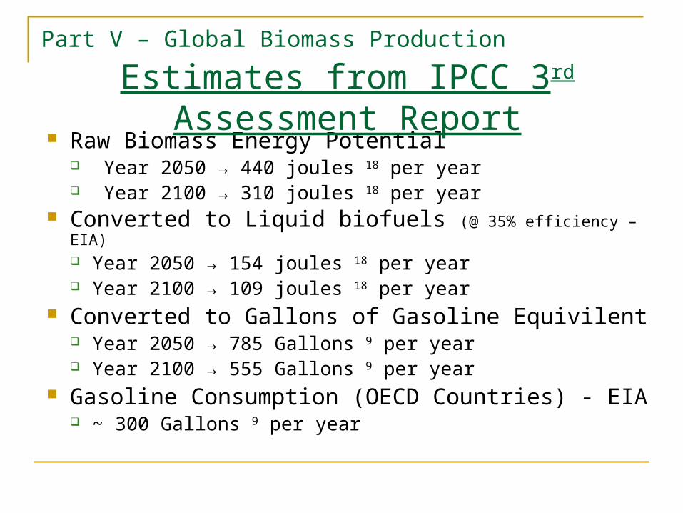
Part V – Global Biomass Production
Raw Biomass Energy Potential Year 2050 → 440 joules 18 per year Year 2100 → 310 joules 18 per year
Converted to Liquid biofuels (@ 35% efficiency – EIA) Year 2050 → 154 joules 18 per year Year 2100 → 109 joules 18 per year
Converted to Gallons of Gasoline Equivilent Year 2050 → 785 Gallons 9 per year Year 2100 → 555 Gallons 9 per year
Gasoline Consumption (OECD Countries) - EIA ~ 300 Gallons 9 per year
Estimates from IPCC 3rd Assessment Report
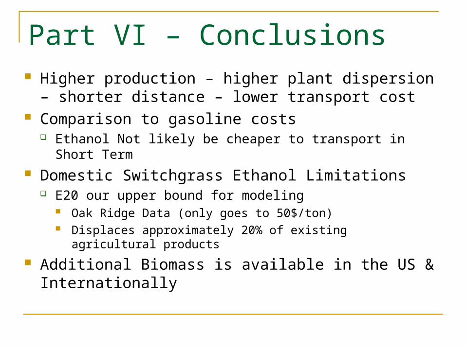
Part VI – Conclusions Higher production – higher plant dispersion –
shorter distance – lower transport cost Comparison to gasoline costs
Ethanol Not likely be cheaper to transport in Short Term Domestic Switchgrass Ethanol Limitations
E20 our upper bound for modeling Oak Ridge Data (only goes to 50$/ton) Displaces approximately 20% of existing agricultural products
Additional Biomass is available in the US & Internationally